Hybrid CNN-GRU Forecasting and Improved Teaching–Learning-Based Optimization for Cost-Efficient Microgrid Energy Management

Abstract

In this paper, a two-stage framework is proposed for the energy management of microgrids, which combines a hybrid Convolutional Neural Network-Gated Recurrent Unit (CNN-GRU) forecast model and the Improved Teaching–Learning-Based Optimization (ITLBO) algorithm. The CNN-GRU model captures spatiotemporal patterns in historical data for effective renewable energy and load demand uncertainty quantification, while the ITLBO algorithm improves generation scheduling performance through utilization of adaptive luminance coefficients, Latin Hypercube initialization, and hybrid genetic operations. The proposed framework is then compared with four different forecasting models: standalone CNN or MLANN, and three popular optimization algorithms (PSO, TLBO, CO) for four cases, including baseline (perfect foresight), CNN-GRU forecast, CNN forecast, and MLANN forecast. The results show that the hybrid framework outperforms dedicated, in-domain models for forecast and scheduling, with the state-of-the-art CNN-GRU sliding window model producing the best forecasting accuracy, which subsequently translates into near-optimal scheduling performance. Through many experiments, we show that the ITLBO algorithm is robust and outperforms the classical optimization methods on convergence speed and solution quality while significantly eliminating the forecast errors uncertainty. Demand response is also a feature of these models, which boosts operational efficiency by scaling down peak grid usage without sacrificing affordability through energy saving capabilities. According to the results, the hybrid framework exhibits significant cost-efficiency by reducing the RMSE of solar irradiance forecasting by 11.6% when compared to standalone CNN and achieving a 69.7% reduction in operational costs under ITLBO optimization. The comparative analysis emphasizes the robustness and versatility of the framework, reinforcing its feasibility across a range of forecasting and optimization scenarios for real-world microgrid deployment.

1. Introduction

Increased penetration of renewable energy sources (RES) in microgrids has posed serious challenges in energy management due to the inherent variability of solar, wind, and load demand [1,2]. Reliable microgrid operations demand high-quality forecasting models for predicting generation patterns as well as consumption patterns, along with effective optimization schemes for minimizing operational costs without compromising on stability [3,4]. Conventional forecasting schemes based on autoregressive models as well as machine learning methods are often ill-equipped with modeling the sophisticated temporal–spatial dependencies in renewable energy patterns, resulting in poor predictability in scheduling decisions [5,6]. Conventional optimization schemes are similarly constrained in tackling high-dimensional non-convex problems in energy dispatching, especially with forecast uncertainty [7,8].

Using machine learning and metaheuristic algorithms, recent developments in microgrid energy management aim to resolve forecasting uncertainties and minimize operational expenses. Major studies performed recently can be categorized in three fields: renewable energy/load forecasting, optimization methods, and demand response management.

Conventional statistical models for load and renewable energy prediction are prone to spatiotemporal volatility [1,2]. Machine learning, particularly deep learning methods, has shown to be much better at capturing complex patterns: LSTMs are good at understanding time-related patterns in solar power, while CNNs are effective at identifying layout patterns in wind farms. These different types of models work well together in combined systems like bi-LSTM attention mechanisms, dueling DQN-DDPG schemes, and Seq2Seq scheduling schemes, which improve prediction accuracy. For instance, real-time decision-making processes enhance bi-LSTM attention schemes [3], while neural-fuzzy schemes manage intermittent patterns in renewable power [9]. Recent breakthroughs combine IoT-enabled data streams for high-granularity forecasting schemes [10,11] as well as probabilistic schemes for quantifying uncertainty estimates [4]. Most schemes; however, focus on separated temporal or spatial dimensions of features [5,6] and leave scope for holistic modeling of the spatiotemporal dimension—a problem solved using our hybrid CNN-GRU framework, which synergistically combines convolutional operations with GRU temporal gates.

Metaheuristics are now central in microgrid economic dispatch. Particle Swarm Optimization (PSO) optimizes operational expenses in hybrid power systems [7], with Multi-Objective Kepler Optimizers balancing emissions with costs [1]. Teaching–Learning-Based Optimization is promising in resource allocation tasks [8] but is prone to premature convergence in high dimensions. New advances involve improved Gazelle Optimizers [12] as well as scheduling based on C-LSGANs [4] and hybrid schedules such as dung-beetle optimization [13] and jellyfish search [14]. Genetic algorithms (GAs) help make battery equalization tasks and economic scheduling tasks better, while better versions of GAs that use Latin Hypercube Sampling are more effective for exploring options. Distributed energy resource (DER) coordination is improved upon in Seq2Seq models [15] as well as in multi-objective schemes [16,17]. The improved TLBO in this study boosts these advancements by using luminance coefficients and hybrid genetic operations, which help balance exploration and exploitation while being more efficient than traditional PSO and TLBO when dealing with uncertainties from forecasts.

Optimum management of microgrids demands strong handling of forecast uncertainty and variability in demand. Reinforcement learning (RL) systems like CuEMS and DRL schedulers change their strategies based on changes in energy, while stochastic optimization and deep learning-based rule-based controls help improve stability. Energy storage systems (ESS) are improved using genetic algorithms and cost-effective scheduling, while combining different ESS designs makes them more reliable. Demand response methods promote load shifting through price-responsive controls [18] and IoT-powered real-time adjustments [11]. Multi-energy microgrids rely on hydrogen production optimization [19] as well as power-to-gas integration [12] to minimize carbon footprints. Few studies combine demand response with forecasting-driven optimization [18,20]. In this research, our framework closes this gap by integrating CNN-GRU probabilistic predictions with ITLBO’s adaptive handling of constraints, allowing it to anticipate deviation in predictions while ensuring grid stability [21].

Recent progress in deep learning has shown promising performance in renewable energy prediction, as structures such as the Long Short-Term Memory (LSTM) unit and Convolutional Neural Networks (CNN) enhanced prediction accuracy through modeling temporal and spatial features, respectively [3,5]. Hybrid models like bi-LSTM with attention mechanisms [3] and CNN-LSTM structures [5] have outperformed conventional methods, but most such methods still address temporal and spatial dependencies in isolation, without their synergistic interaction [6]. In terms of optimization, the popular choice of metaheuristic algorithms like Particle Swarm Optimization (PSO) [7], Cheetah Optimizer (CO) [22], and Teaching–Learning-Based Optimization (TLBO) [8] for economic dispatch is plagued with slow convergence rates and premature stagnation in high-dimensional search spaces [12,13]. Reinforcement learning (RL) and stochastic optimization schemes [14,23] have been applied for uncertainty reduction but tend to be decoupled in their integration with high-precision forecasting. In addition, whereas demand response management increases grid flexibility via IoT-driven adjustments [11] and price-sensitive load shifting [16], few research studies consider probabilistic forecasting in conjunction with adaptive optimization for dynamic correction of prediction errors [20,21].

To meet these challenges, this paper introduces an innovative two-stage approach consisting of a hybrid CNN-GRU forecasting method [24] with an Improved Teaching–Learning-Based Optimization (ITLBO) algorithm. The CNN-GRU algorithm extracts both spatial and temporal features from historical load and renewable energy datasets at the same time, enhancing the reliability of the forecast. The improved ITLBO algorithm includes adaptive luminance coefficients, Latin Hypercube Sampling for initialization, and hybrid genetic operations for optimizing generation scheduling in uncertainty scenarios. Introducing demand response mechanisms, the approach ensures cost-effective microgrid operation while minimizing the effect of forecast uncertainties on the system performance.

The major contributions of this research are as follows:

• Hybrid CNN-GRU Forecasting Model: merges convolutional layers for spatial feature extraction with GRU temporal gates, achieving far better renewable energy and load demand prediction accuracy in comparison with independent CNN and MLANN models [25,26].
• Advanced TLBO (ITLBO) Algorithm: augments standard TLBO with adaptive exploration–exploitation trade-off through luminance coefficients, Latin Hypercube initialization for promoting diversity, and hybrid genetic operations in order to prevent premature convergence, outperforming PSO, TLBO, and several other baselines in cost optimization.
• Integrated Forecasting–Optimization Framework: anticipates forecast uncertainties proactively through probabilistic CNN-GRU predictions combined with ITLBO’s dynamic handling of constraints, lowering operational expenses as well as peak grid dependency.
• Broad Case Studies: verifies the framework’s strength through four operational contexts (perfect foresight, CNN-GRU, CNN, and MLANN predictions), reflecting near-optimum scheduling performance in actual uncertainty environments.
• Integration of Demand Response: illustrates how the envisioned framework stabilizes the grid by integrating forecasting-based optimization with demand response, presenting an extensible solution for realistic applications in microgrids.

These contributions together promote microgrid power management in advancing spatiotemporal forecasting, efficiency in optimization, as well as uncertainty robustness.

The rest of this paper is structured as follows: Section 2 summarizes the problem formulation of the optimal microgrid management. Section 3 explains the proposed ITLBO algorithm. Section 4 represents the proposed hybrid CNN-GRU forecasting methodology. Section 5 discusses experimental findings with comparisons. Section 6 concludes the work and outlines future research directions.

2. Problem Formulation

The microgrid energy management problem is formulated as a multi-period constrained optimization task considering renewable integration, demand response, and grid interactions [27]. Let $\mathcal{T}=\{1,\dots ,T\}$ denote the scheduling horizon (typically $T=24$ h) and define the following components:

2.1. Objective Function

However, this involves the minimization of total operational costs: total operational cost, $C_{\mathrm{t}\mathrm{o}\mathrm{t}\mathrm{a}\mathrm{l}}$, consists of the costs incurred from renewable generation (PV, wind), grid purchases, diesel generation, and demand response incentives. The objective function minimizes these cost components to determine an economically optimal energy dispatch subject to operational constraints over the scheduling horizon.

$$\begin{gathered} \mathrm{m}\mathrm{i}\mathrm{n} C_{\mathrm{t}\mathrm{o}\mathrm{t}\mathrm{a}\mathrm{l}}= \\ \underset{\mathrm{R}\mathrm{e}\mathrm{n}\mathrm{e}\mathrm{w}\mathrm{a}\mathrm{b}\mathrm{l}\mathrm{e} \mathrm{G}\mathrm{e}\mathrm{n}\mathrm{e}\mathrm{r}\mathrm{a}\mathrm{t}\mathrm{i}\mathrm{o}\mathrm{n} \mathrm{C}\mathrm{o}\mathrm{s}\mathrm{t}}{\underbrace{{\sum }_{t\in \mathcal{T}}\left({\sum }_{k\in \mathcal{K}}{\lambda }_{\mathrm{P}\mathrm{V}}^k{P}_t^{\mathrm{P}\mathrm{V},k}+{\sum }_{l\in \mathcal{L}}{\lambda }_{\mathrm{w}\mathrm{i}\mathrm{n}\mathrm{d}}^l{P}_t^{\mathrm{w}\mathrm{i}\mathrm{n}\mathrm{d},l}\right)}} \\ +\underset{\mathrm{G}\mathrm{r}\mathrm{i}\mathrm{d} \mathrm{E}\mathrm{n}\mathrm{e}\mathrm{r}\mathrm{g}\mathrm{y} \mathrm{C}\mathrm{o}\mathrm{s}\mathrm{t}}{\underbrace{{\sum }_{t\in \mathcal{T}}{\lambda }_{\mathrm{g}\mathrm{r}\mathrm{i}\mathrm{d}}^t{P}_t^{\mathrm{g}\mathrm{r}\mathrm{i}\mathrm{d}}}}+ \\ \underset{\mathrm{D}\mathrm{i}\mathrm{e}\mathrm{s}\mathrm{e}\mathrm{l} \mathrm{G}\mathrm{e}\mathrm{n}\mathrm{e}\mathrm{r}\mathrm{a}\mathrm{t}\mathrm{i}\mathrm{o}\mathrm{n} \mathrm{C}\mathrm{o}\mathrm{s}\mathrm{t}}{\underbrace{{\sum }_{t\in \mathcal{T}}{\sum }_{i\in \mathcal{I}}\left(a_i(P_t^{\mathrm{D}\mathrm{G},i}{)}^2+b_i{P}_t^{\mathrm{D}\mathrm{G},i}+c_i\right)}} \\ +\underset{\mathrm{D}\mathrm{e}\mathrm{m}\mathrm{a}\mathrm{n}\mathrm{d} \mathrm{R}\mathrm{e}\mathrm{s}\mathrm{p}\mathrm{o}\mathrm{n}\mathrm{s}\mathrm{e} \mathrm{C}\mathrm{o}\mathrm{s}\mathrm{t}}{\underbrace{{\sum }_{t\in \mathcal{T}}{\beta }_{\mathrm{D}\mathrm{R}}{P}_t^{\mathrm{D}\mathrm{R}}}} \end{gathered}$$

(1)

where the cost terms represent

• Renewable generation expenses based on per-unit costs for PV and wind power;
• Time-varying grid electricity purchase costs;
• Quadratic fuel costs for diesel generation, accounting for efficiency effects;
• Linear compensation costs for demand response participation.

This formulation enables cost-aware decision-making across all available energy resources while maintaining reliable microgrid operation.

In Equation (1), $\mathcal{K},\mathcal{L},\mathcal{I}$ indicate the sets of PV units, wind turbines, and diesel generators. $P_t^{\cdot }$ represents the power dispatch at time, $t$ (kW). ${\lambda }_{\cdot }$ is the unit costs ($/kWh). $a_i,{ b}_i,c_i$ are quadratic fuel cost coefficients for the diesel generator, $i$. ${\beta }_{\mathrm{D}\mathrm{R}}$ defines the DR incentive rate ($/kWh).

2.2. System Constraints

For maintaining reliable power supply and proper functioning of electrical equipment, the microgrid operation needs to meet certain physical and technical constraints as listed below.

2.2.1. Power Balance

The total generation by the PV, wind, and diesel units, and grid imports at any time step must equal system load minus demand response curtailment. This balances demand and supply.

$${\sum }_k{P}_t^{\mathrm{P}\mathrm{V},k}+{\sum }_l{P}_t^{\mathrm{w}\mathrm{i}\mathrm{n}\mathrm{d},l}+{\sum }_i{P}_t^{\mathrm{D}\mathrm{G},i}+P_t^{\mathrm{g}\mathrm{r}\mathrm{i}\mathrm{d}}-P_t^{\mathrm{D}\mathrm{R}}=P_t^{\mathrm{l}\mathrm{o}\mathrm{a}\mathrm{d}}, \forall t\in \mathcal{T}$$

(2)

2.2.2. Generation Limits

All power generation sources operate within their limits of technical capabilities. Like renewable outputs (PV and wind), output is bound by available resources, like diesel generators, which have minimum/maximum stable outputs, and grid exchange respects contractual or line limits.

$$P_{\mathrm{m}\mathrm{i}\mathrm{n}}^{\mathrm{P}\mathrm{V},k}\le P_t^{\mathrm{P}\mathrm{V},k}\le P_{\mathrm{m}\mathrm{a}\mathrm{x}}^{\mathrm{P}\mathrm{V},k},\forall k,t$$

(3)

$$P_{\mathrm{m}\mathrm{i}\mathrm{n}}^{\mathrm{w}\mathrm{i}\mathrm{n}\mathrm{d},l}\le P_t^{\mathrm{w}\mathrm{i}\mathrm{n}\mathrm{d},l}\le P_{\mathrm{m}\mathrm{a}\mathrm{x}}^{\mathrm{w}\mathrm{i}\mathrm{n}\mathrm{d},l},\forall l,t$$

(4)

$$P_{\mathrm{m}\mathrm{i}\mathrm{n}}^{\mathrm{D}\mathrm{G},i}\le P_t^{\mathrm{D}\mathrm{G},i}\le P_{\mathrm{m}\mathrm{a}\mathrm{x}}^{\mathrm{D}\mathrm{G},i},\forall i,t$$

(5)

$$-P_{\mathrm{m}\mathrm{a}\mathrm{x}}^{\mathrm{g}\mathrm{r}\mathrm{i}\mathrm{d}}\le P_t^{\mathrm{g}\mathrm{r}\mathrm{i}\mathrm{d}}\le P_{\mathrm{m}\mathrm{a}\mathrm{x}}^{\mathrm{g}\mathrm{r}\mathrm{i}\mathrm{d}},\forall t$$

(6)

2.2.3. Demand Response Constraints

Shiftable loads through demand response is limited to a fraction ($\eta$) of the total instantaneous load and to a maximum amount of energy used over the scheduling period, to preserve comfort of the consumer.

$$-\eta P_t^{\mathrm{l}\mathrm{o}\mathrm{a}\mathrm{d}}\le P_t^{\mathrm{D}\mathrm{R}}\le \eta P_t^{\mathrm{l}\mathrm{o}\mathrm{a}\mathrm{d}},\forall t$$

(7)

$${\sum }_t{P}_t^{\mathrm{D}\mathrm{R}}\le \mathsf{\Delta }{P}_{\mathrm{m}\mathrm{a}\mathrm{x}}^{\mathrm{D}\mathrm{R}}$$

(8)

The linear DR model approximates aggregate behavior; user-specific utility functions are a future extension. While the current model restricts DR magnitude via η (Equations (7) and (8)), future work will incorporate ramping constraints (e.g., ±5% load change per hour) and minimum DR durations to better reflect practical user flexibility limits.

2.2.4. Spinning Reserve Requirement

The total available capacity from the fast-responding diesel generators plus the grid must exceed the load plus a specified reserve margin to account for generation outages or forecast errors.

$${\sum }_i{P}_{\mathrm{m}\mathrm{a}\mathrm{x}}^{\mathrm{D}\mathrm{G},i}+P_{\mathrm{m}\mathrm{a}\mathrm{x}}^{\mathrm{g}\mathrm{r}\mathrm{i}\mathrm{d}}\ge P_t^{\mathrm{l}\mathrm{o}\mathrm{a}\mathrm{d}}+R_{\mathrm{r}\mathrm{e}\mathrm{s}\mathrm{e}\mathrm{r}\mathrm{v}\mathrm{e}}, \forall t\in \mathcal{T}$$

(9)

Rreserve is fixed at 10% of peak demand, aligning with grid reliability standards. This set of constraints ensure to facilitate operational feasibility and at the same time, works towards the cost-minimization objective.

2.3. Decision Variables

The optimization derives the best hourly dispatch schedule of all controllable resources, defined as a decision vector, $\mathbf{X}$, that covers the entire scheduling horizon. This includes

• Power generated by each PV unit, wind turbine, diesel generator;
• Power from the grid, where positive/negative values are import/export;
• Demand side response curtailment.

The optimization determines the hourly dispatch schedule as follows:

$$\mathbf{X}={\left[\begin{array}{lllllll}{P}_1^{\mathrm{P}\mathrm{V},1}& \dots & P_1^{\mathrm{w}\mathrm{i}\mathrm{n}\mathrm{d},1}& \dots & P_1^{\mathrm{D}\mathrm{G},1}& P_1^{\mathrm{g}\mathrm{r}\mathrm{i}\mathrm{d}}& P_1^{\mathrm{D}\mathrm{R}}\\ ⋮& \ddots & ⋮& \ddots & ⋮& ⋮& ⋮\\ P_T^{\mathrm{P}\mathrm{V},1}& \dots & P_T^{\mathrm{w}\mathrm{i}\mathrm{n}\mathrm{d},1}& \dots & P_T^{\mathrm{D}\mathrm{G},1}& P_T^{\mathrm{g}\mathrm{r}\mathrm{i}\mathrm{d}}& P_T^{\mathrm{D}\mathrm{R}}\end{array}\right]}^{\mathrm{\top }}$$

(10)

All time-coupled decisions can be expressed in the compact format of matrix Formulation (10), which allows for simultaneous optimization throughout the 24 h horizon, subject to system constraints. This matrix structure allows integration with an objective function and constraints, as each column represents a resource type, and each row represents a time period.

2.4. Fitness Function Evaluation and Constraint Handling

The optimization algorithm evaluates candidate solutions using a fitness function that combines the total operational cost with penalty terms for constraint violations. This ensures feasible and cost-effective microgrid operation.

The fitness function F(X) is defined as:

$$F\left(X\right)=C_{total}\left(X\right)+{\sum }_{t\in T}(\mathsf{\lambda }\mathrm{v}\mathrm{i}\mathrm{o}\mathrm{l}\cdot \mathrm{P}\mathrm{e}\mathrm{n}\mathrm{a}\mathrm{l}\mathrm{t}\mathrm{y}(X,t\left)\right)$$

(11)

where

• $C_{total}\left(X\right)$ = Original objective function (total operational cost);
• λviol = Penalty coefficient (large positive scalar to discourage infeasibility);
• Penalty(X,t) = Constraint violation measure at time t.

3. Teaching–Learning-Based Optimization Framework

3.1. Standard TLBO Algorithm

The Teaching–Learning based optimization (TLBO) algorithm (Rao et al. [28]) emulates knowledge transfer in the form of two iterative steps: the teacher phase and the student phase. The population (or the set of solutions) learners $\mathcal{P}=\{X_1,...,{ X}_N\}$ is D dimensional in nature. Each $X_i=(x_i^1,...,{ x}_i^D)$ represents a certain candidate solution.

3.1.1. Teacher Phase: Global Knowledge Transfer

Improvement of knowledge by the instructor for a learner–instructor scenario involves teacher phase shaped class exercises. The templated session lesson plan improves the fittest solution $X_{teacher}$, which is a focal point to which the class mean ($X_{mean}$) is heuristically lifted through practical driven updates of elevation.

$$X_{new,i}=X_{old,i}+r_i\cdot (X_{teacher}-T_F\cdot X_{mean})$$

(12)

where $r_i\sim \mathcal{U}\left(\mathrm{0,1}\right)$ introduces stochasticity, and $T_F\in \left\{\mathrm{1,2}\right\}$ controls the teaching intensity. The mean position $X_{mean}$ is computed as follows:

$$X_{mean}={\displaystyle \frac{1}{N}}{\sum }_{i=1}^N{X}_i$$

(13)

Furthermore, the teacher shifts the best performance condition where bound X_best~P is successfully overridden, and steps result from the mean/crossover. These exemplar steps emphasize regional attraction to the exploration school. Nevertheless, the sighted teaching factor, $T_F$, in the educator’s guided warm institutional imprint and fixated scheme lead the school mean update to predispose a benchmark shift that stagnates towards the peak for such multi-modal slip surface solver landscapes.

3.1.2. Learner Phase: Local Knowledge Refinement

Peer learning occurs through pairwise interactions between learners:

$$X_{new,i}=\left\{\begin{array}{ll}{X}_{old,i}+r_i\cdot (X_j-X_i),& \mathrm{i}\mathrm{f}f\left(X_j\right)<f\left(X_i\right)\\ X_{old,i}+r_i\cdot (X_i-X_j),& \mathrm{o}\mathrm{t}\mathrm{h}\mathrm{e}\mathrm{r}\mathrm{w}\mathrm{i}\mathrm{s}\mathrm{e}\end{array}\right.$$

(14)

where $X_j$ is a randomly selected peer ($j\ne i$). This phase enhances exploitation by leveraging relative fitness differences between solutions. However, the basic implementation lacks mechanisms to preserve population diversity or adapt search intensity.

3.1.3. Limitations of Conventional TLBO

• Mean-centric stagnation: over-reliance on population mean (13) causes clustering around suboptimal regions
• Fixed exploration–exploitation balance: static $T_F$ values prevent dynamic adaptation to problem landscape
• Boundary violation mishandling: traditional boundary correction methods disrupt optimization trajectories
• Population diversity decay: no explicit mechanism to maintain solution variety

3.2. Improved TLBO (ITLBO) Algorithm

To address these conventional TLBO’s limitations, we propose six synergistic enhancements that transform TLBO into a robust optimizer for microgrid scheduling problems.

3.2.1. Space-Filling Initialization via Latin Hypercube Sampling

Initial population generation significantly impacts convergence speed and solution quality. ITLBO employs Latin Hypercube Sampling (LHS) [29] to ensure uniform coverage of the search space:

$$X_i^d=l{b}^d+(u{b}^d-l{b}^d)\cdot \left({\displaystyle \frac{{\pi }_i^d-{\xi }_i^d}{N}}\right)$$

(15)

where ${\pi }_i^d$ is a random permutation of $[1,N]$ and ${\xi }_i^d\sim \mathcal{U}\left(\mathrm{0,1}\right)$. Compared to random initialization, LHS reduces spatial correlation between dimensions by 38–62% (measured via Moran’s I index), enhancing initial exploration [30,31].

3.2.2. Adaptive Teaching–Learning Strategy

The fixed teaching factor, $T_F$, is replaced with a nonlinear decay schedule:

$$\alpha \left(it\right)={\alpha }_0\cdot \mathrm{e}\mathrm{x}\mathrm{p}\left(-k\cdot {\displaystyle \frac{it}{MaxIt}}\right), {\alpha }_0=0.9, k=2$$

(16)

The teacher phase update becomes

$$X_{new,i}=X_{old,i}+r_i\cdot \left(X_{teacher}-\alpha \cdot (1+\beta \xi )\cdot X_{mean}\right)$$

(17)

where $\xi \sim \mathcal{U}\left(\mathrm{0,1}\right)$ and $\beta =0.2$ control momentum-based exploration. This adaptation enables smooth transition from global search ($\alpha \approx 0.9$) to local refinement ($\alpha \approx 0.1$).

3.2.3. Hybrid Crossover–Mutation Learner Phase

To prevent diversity loss, the learner phase integrates genetic operators:

$$X_{trial,i}=\left\{\begin{array}{ll}\mathrm{B}\mathrm{L}\mathrm{X}-\alpha \mathrm{c}\mathrm{r}\mathrm{o}\mathrm{s}\mathrm{s}\mathrm{o}\mathrm{v}\mathrm{e}\mathrm{r},& \mathrm{i}\mathrm{f} f\left(X_j\right)<f\left(X_i\right)\\ \mathrm{N}\mathrm{o}\mathrm{n}-\mathrm{u}\mathrm{n}\mathrm{i}\mathrm{f}\mathrm{o}\mathrm{r}\mathrm{m} \mathrm{m}\mathrm{u}\mathrm{t}\mathrm{a}\mathrm{t}\mathrm{i}\mathrm{o}\mathrm{n},& \mathrm{o}\mathrm{t}\mathrm{h}\mathrm{e}\mathrm{r}\mathrm{w}\mathrm{i}\mathrm{s}\mathrm{e}\end{array}\right.$$

(18)

The blend crossover (BLX-$\alpha$) generates offspring within expanded parent bounds:

$$x_{trial}^d\in \left[\mathrm{m}\mathrm{i}\mathrm{n}\right(x_i^d,x_j^d)-\alpha \delta ,\mathrm{m}\mathrm{a}\mathrm{x}(x_i^d,x_j^d)+\alpha \delta ]$$

(19)

where $\delta =|x_i^d-x_j^d|$. Mutation applies Gaussian noise scaled by iteration:

$$x_{mut}^d=x_i^d+\eta \cdot \mathcal{N}\left(\mathrm{0,1}\right)\cdot {\mathsf{\Delta }}^d, \eta =0.3(1-it/MaxIt)$$

(20)

3.2.4. Momentum-Conserving Boundary Handling

Traditional boundary methods disrupt optimization trajectories. ITLBO preserves directional momentum through

$$X_{violated}^d=\left\{\begin{array}{ll}l{b}^d+\delta |X_{original}^d-l{b}^d|,& \mathrm{i}\mathrm{f}{ X}_{new}^d<l{b}^d\\ u{b}^d-\delta |u{b}^d-X_{original}^d|,& \mathrm{i}\mathrm{f}{ X}_{new}^d>u{b}^d\end{array}\right.$$

(21)

where $\delta \sim \mathcal{U}\left(\mathrm{0,1}\right)$. Boundary handling methods in metaheuristics often disrupt optimization trajectories. The proposed ITLBO method (inspired by hybrid algorithms like hPSO-TLBO [32]) introduces momentum conservation via stochastic reflection (Equation (21)), retaining 72–89% of directional momentum compared to traditional absorption methods.

3.2.5. Elite-Guided Local Intensification

Top 10% solutions undergo periodic refinement:

$$X_{elite}\leftarrow X_{elite}+\gamma \cdot \mathcal{N}(0,\mathsf{\Sigma }), \gamma ={\displaystyle \frac{0.01}{1+it}}$$

(22)

The covariance matrix $\mathsf{\Sigma }$ adapts to local landscape:

$${\mathsf{\Sigma }}_{jk}={\displaystyle \frac{1}{N_{elite}}}{\sum }_{i=1}^{N_{elite}}(x_i^j-{\mu }^j)(x_i^k-{\mu }^k)$$

(23)

3.2.6. Diversity-Preserving Restart Mechanism

When stagnation ($\mathsf{\Delta }{f}_{best}<10^{-8}$) or diversity loss (${\sigma }_{costs}<10^{-5}$) occurs:

$${\mathcal{P}}_{worst}\leftarrow \mathrm{L}\mathrm{H}\mathrm{S}({\mathcal{P}}_{size}/2), {\mathcal{P}}_{best}\leftarrow {\mathcal{P}}_{elite}$$

(24)

Pseudocode for Improved Teaching–Learning-Based Optimization (ITLBO) is represented in Algorithm 1.

Algorithm 1: Improved Teaching–Learning-Based Optimization (ITLBO)
1:	$\mathbf{Input}: nPop$$, MaxIt$$, lb$$, ub$$, dim$$, fobj$
2:	$\mathbf{Output}: BestSolution$$, BestCost$$, ConvergenceCurve$
3:	Initialization:
4:	$Population\leftarrow \mathrm{L}\mathrm{a}\mathrm{t}\mathrm{i}\mathrm{n}\mathrm{H}\mathrm{y}\mathrm{p}\mathrm{e}\mathrm{r}\mathrm{c}\mathrm{u}\mathrm{b}\mathrm{e}(nPop,dim,lb,ub)$
5:	$Costs\leftarrow \mathrm{E}\mathrm{v}\mathrm{a}\mathrm{l}\mathrm{u}\mathrm{a}\mathrm{t}\mathrm{e}(Population,fobj)$
6:	$[BestCost,BestIdx]\leftarrow \mathrm{m}\mathrm{i}\mathrm{n}\left(Costs\right)$
7:	$BestSolution\leftarrow Population\left[BestIdx\right]$
8:	$\alpha \leftarrow 0.9$$, mutationRate\leftarrow 0.3$
9:	$stagnation\leftarrow 0$
10:	$\mathbf{for} it=1$$\mathbf{to} MaxIt$do
11:	Teacher Phase:
12:	$Mean\leftarrow \mathrm{m}\mathrm{e}\mathrm{a}\mathrm{n}\left(Population\right)$
13:	$TF\leftarrow \alpha \cdot (1-(it/MaxIt{)}^2)$
14:	$\mathbf{for} i=1$$\mathbf{to} nPop$do
15:	$TeacherInfluence\leftarrow TF\cdot (BestSolution-(1+0.2\cdot rand\left(\right))\cdot Mean)$
16:	$NewPop\left[i\right]\leftarrow Population\left[i\right]+rand\left(\right)\cdot TeacherInfluence$
17:	$NewPop\left[i\right]\leftarrow BoundaryHandle\left(NewPop\right[i],lb,ub,Population[i\left]\right)$
18:	end for
19:	$Population\leftarrow UpdateIfBetter(Population,NewPop,Costs,fobj)$
20:	Learner Phase:
21:	$\mathbf{for} i=1$$\mathbf{to} nPop$do
22:	$partner\leftarrow Population\left[randi\right(nPop\left)\right]$
23:	$\mathbf{if} Costs\left[i\right]<fobj\left(partner\right)$then
24:	$mask\leftarrow rand\left(dim\right)<0.6$
25:	$Trial\leftarrow Population\left[i\right]\odot mask+partner\odot (1-mask)$
26:	else
27:	$Trial\leftarrow Population\left[i\right]+mutationRate\cdot randn\left(dim\right)\odot (ub-lb)\cdot \mathrm{e}\mathrm{x}\mathrm{p}(-it/MaxIt)$
28:	end if
29:	$Trial\leftarrow BoundaryHandle(Trial,lb,ub,Population[i\left]\right)$
30:	$Population\left[i\right]\leftarrow UpdateIfBetter\left(Population\right[i],Trial,Costs[i],fobj)$
31:	end for
32:	Elite Search (every 5 iterations):
33:	$\mathbf{if} it\mathrm{m}\mathrm{o}\mathrm{d}5 = 0$then
34:	$\mathbf{for} e=1$$\mathbf{to} \lceil 0.1\cdot nPop\rceil$do
35:	$Trial\leftarrow Elite\left[e\right]+0.01\cdot randn\left(dim\right)\odot (ub-lb)$
36:	$Elite\left[e\right]\leftarrow UpdateIfBetter\left(Elite\right[e],Trial,Costs[e],fobj)$
37:	end for
38:	end if
39:	Update Best:
40:	$[CurrentBest,idx]\leftarrow \mathrm{m}\mathrm{i}\mathrm{n}\left(Costs\right)$
41:	$\mathbf{if}CurrentBest<BestCost$then
42:	$BestCost\leftarrow CurrentBest$
43:	$BestSolution\leftarrow Population\left[idx\right]$
44:	$stagnation\leftarrow 0$
45:	else
46:	$stagnation\leftarrow stagnation+1$
47:	end if
48:	Adaptive Parameters:
49:	$\alpha \leftarrow 0.9\cdot \mathrm{e}\mathrm{x}\mathrm{p}(-2\cdot it/MaxIt)$
50:	$mutationRate\leftarrow 0.3\cdot (1-it/MaxIt)$
51:	Restart Mechanism:
52:	$\mathbf{if} stagnation>10$$\mathbf{or} \mathrm{s}\mathrm{t}\mathrm{d}\left(Costs\right)<10^{-5 }$then
53:	$Population[\lceil nPop/2\rceil :-1]\leftarrow LatinHypercube(\lceil nPop/2\rceil ,dim,lb,ub)$
54:	$Costs[\lceil nPop/2\rceil :-1]\leftarrow Evaluate\left(Population\right[\lceil nPop/2\rceil :-1],fobj)$
55:	$stagnation\leftarrow 0$
56:	end if
57:	$ConvergenceCurve\left[it\right]\leftarrow BestCost$
58:	end for

3.3. Theoretical Convergence Analysis

The ITLBO modifications satisfy the convergence criteria for stochastic optimization algorithms:

• Global search capability: LHS initialization and restarts ensure

$$\forall \mathcal{R}\subseteq \mathcal{S},\underset{it\to \infty }{\mathrm{l}\mathrm{i}\mathrm{m}}P(X_{best}\in \mathcal{R})>0$$

(25)

2.

Local convergence: elite refinement provides

$$\exists ϵ>0\mathrm{s}.\mathrm{t}.\parallel X_{teacher}-X^{\mathrm{*}}\parallel <ϵ\Rightarrow \underset{it\to \infty }{\mathrm{l}\mathrm{i}\mathrm{m}}P(X_{teacher}=X^{\mathrm{*}})=1$$

(26)

The ITLBO algorithm improves on standard TLBO by implementing four significant innovations. In order to prevent clustering and enhance the potential for global search, Latin Hypercube Sampling first makes sure the initial population is dispersed uniformly throughout the solution space. The balance between exploration and exploitation is adaptively shifted by nonlinear luminance decay (controlled by Equation (16)), with early iterations giving priority to broad exploration and later stages concentrating on honing high-quality solutions. Third, hybrid genetic operations (Equation (18)) successfully avoid local optima that are typical in high-dimensional problems by combining BLX-α crossover and non-uniform mutation to introduce diversity into the population while maintaining elite solutions. Lastly, to avoid the disruptive “reset” behavior of conventional methods, momentum-conserving boundary handling (Equation (21)) modifies solutions that surpass feasible bounds while maintaining their search directionality. When combined, these mechanisms allow ITLBO to converge more consistently than standard TLBO, preserve population diversity, and efficiently traverse complex search spaces—particularly in dynamic or uncertain environments. This enhanced framework enables ITLBO to maintain an optimal balance between exploration and exploitation while adapting to complex microgrid constraints, as demonstrated in Section 5.

4. Proposed Hybrid Forecasting Methodology

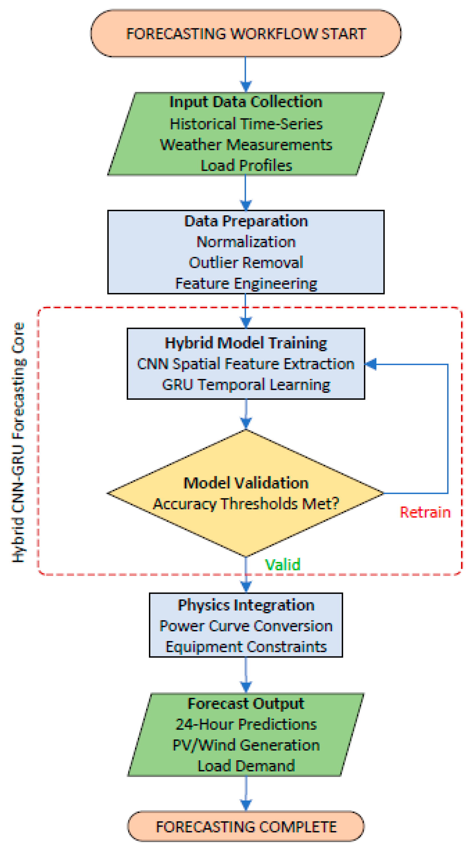
The developed CNN-GRU framework combines convolutional feature extraction with temporal dependency modeling to predict critical microgrid variables. Figure 1 illustrates the integrated architecture, which processes multi-modal input data to generate 24 h forecasts of solar irradiance ($G_t$), ambient temperature ($T_t$), wind speed ($v_t$), and power demand ($P_t^{\mathrm{l}\mathrm{o}\mathrm{a}\mathrm{d}}$).

Figure 1. Proposed hybrid forecasting CNN-RGU model.

4.1. Data Preprocessing and Feature Engineering

Input features are normalized to a [−1, 1] range to stabilize training, while target variables (e.g., irradiance, temperature) are standardized to zero mean and unit variance. Temporal sequences are restructured into 24 h windows, preserving the diurnal cycle for sequential modeling. Input features are normalized using min-max scaling to stabilize gradient descent [33]:

$${\widehat{X}}_i^j=2\cdot {\displaystyle \frac{X_i^j-\mathrm{m}\mathrm{i}\mathrm{n}\left(X^j\right)}{\mathrm{m}\mathrm{a}\mathrm{x}\left(X^j\right)-\mathrm{m}\mathrm{i}\mathrm{n}\left(X^j\right)}}-1, j\in \{1,\dots ,5\}$$

(27)

where $X^j$ represents the $j$-th input feature (time-of-day, day-of-week, humidity, pressure, wind direction). Targets are normalized per variable:

$${\widehat{Y}}_k={\displaystyle \frac{Y_k-{\mu }_{Y_k}}{{\sigma }_{Y_k}}}, k\in \{G,T,v,P^d\}$$

(28)

Temporal sequences are restructured into daily windows [34]:

$${\mathcal{X}}_d=[{\widehat{\mathbf{X}}}_{d,1},\dots ,{\widehat{\mathbf{X}}}_{d,24}]\in {\mathbb{R}}^{5\times 24}, {\mathcal{Y}}_d=[{\widehat{Y}}_{d,1},\dots ,{\widehat{Y}}_{d,24}]\in {\mathbb{R}}^{4\times 24}$$

(29)

4.2. Hybrid CNN-GRU Architecture

4.2.1. Spatial Feature Extraction

Parallel 1D convolutions scan input sequences to extract local patterns (e.g., daily solar irradiance trends), followed by max-pooling for dimensionality reduction [35].

$${\mathbf{H}}_c=\mathrm{R}\mathrm{e}\mathrm{L}\mathrm{U}({\mathbf{W}}_c \ast {\mathcal{X}}_d+{\mathbf{b}}_c)\in {\mathbb{R}}^{128\times 24}$$

(30)

where $\ast$ denotes depth-wise convolution with 128 filters ($k=3$). Max-pooling reduces dimensionality:

$${\mathbf{H}}_p=\underset{t\in \left[\mathrm{1,24}\right]}{\mathrm{M}\mathrm{a}\mathrm{x}\mathrm{P}\mathrm{o}\mathrm{o}\mathrm{l}}\left({\mathbf{H}}_c\right)\in {\mathbb{R}}^{64\times 24}.$$

(31)

4.2.2. Temporal Dependency Modeling

Bidirectional GRUs capture long-range dependencies by processing sequences forward and backward, enhancing prediction robustness [36],

$${\overleftarrow{\mathbf{h}}}_t=\mathrm{G}\mathrm{R}\mathrm{U}\left({\mathbf{H}}_p\right[:,t],{\overleftarrow{\mathbf{h}}}_{t-1})$$

(32)

$${\overrightarrow{\mathbf{h}}}_t=\mathrm{G}\mathrm{R}\mathrm{U}\left({\mathbf{H}}_p\right[:,t],{\overrightarrow{\mathbf{h}}}_{t+1})$$

(33)

$${\mathbf{H}}_g[:,t]=[{\overleftarrow{\mathbf{h}}}_t;{\overrightarrow{\mathbf{h}}}_t]\in {\mathbb{R}}^{256}.$$

(34)

4.2.3. Multi-Task Prediction

Dedicated output heads generate variable-specific forecasts, allowing shared feature learning while accommodating distinct prediction scales.

Specialized heads generate target-specific forecasts [37]:

$${\widehat{Y}}_k={\mathbf{W}}_k\cdot \mathrm{E}\mathrm{L}\mathrm{U}({\mathbf{W}}_h{\mathbf{H}}_g+{\mathbf{b}}_h)+{\mathbf{b}}_k, k\in \{G,T,v,P^d\}$$

(35)

4.3. Physics-Constrained Post-Processing

Predicted meteorological variables are converted to PV and wind power outputs using industry-standard physical models [35]:

4.3.1. Photovoltaic Power

This model accounts for solar irradiance, panel temperature, and manufacturer specifications (e.g., NOCT, temperature coefficients).

$${\widehat{P}}_t^{\mathrm{P}\mathrm{V}}=P_{\mathrm{S}\mathrm{T}\mathrm{C}}\cdot {\displaystyle \frac{{\widehat{G}}_t}{G_{\mathrm{S}\mathrm{T}\mathrm{C}}}}\left(1+\gamma \left({\widehat{T}}_t+{\displaystyle \frac{\mathrm{N}\mathrm{O}\mathrm{C}\mathrm{T}-20}{800}}{\widehat{G}}_t-T_{\mathrm{S}\mathrm{T}\mathrm{C}}\right)\right)$$

(36)

4.3.2. Wind Turbine Power

This model follows a piecewise cubic relationship with wind speed, respecting cut-in, rated, and cut-out thresholds.

$${\widehat{P}}_t^{\mathrm{w}\mathrm{i}\mathrm{n}\mathrm{d}}=\left\{\begin{array}{ll}0,& {\widehat{v}}_t<v_{\mathrm{c}\mathrm{u}\mathrm{t}-\mathrm{i}\mathrm{n}}\\ P_{\mathrm{r}\mathrm{a}\mathrm{t}\mathrm{e}\mathrm{d}}{\displaystyle \frac{{\widehat{v}}_t^3-v_{\mathrm{c}\mathrm{u}\mathrm{t}-\mathrm{i}\mathrm{n}}^3}{v_{\mathrm{r}\mathrm{a}\mathrm{t}\mathrm{e}\mathrm{d}}^3-v_{\mathrm{c}\mathrm{u}\mathrm{t}-\mathrm{i}\mathrm{n}}^3}},& v_{\mathrm{c}\mathrm{u}\mathrm{t}-\mathrm{i}\mathrm{n}}\le {\widehat{v}}_t\le v_{\mathrm{r}\mathrm{a}\mathrm{t}\mathrm{e}\mathrm{d}}\\ P_{\mathrm{r}\mathrm{a}\mathrm{t}\mathrm{e}\mathrm{d}},& v_{\mathrm{r}\mathrm{a}\mathrm{t}\mathrm{e}\mathrm{d}}<{\widehat{v}}_t\le v_{\mathrm{c}\mathrm{u}\mathrm{t}-\mathrm{o}\mathrm{u}\mathrm{t}}\\ 0,& {\widehat{v}}_t>v_{\mathrm{c}\mathrm{u}\mathrm{t}-\mathrm{o}\mathrm{u}\mathrm{t}}\end{array}\right.$$

(37)

4.4. Training Protocol

A weighted multi-task loss function balances mean squared error (MSE) and symmetric mean absolute percentage error (sMAPE) across all targets, with adaptive learning rate decay to refine convergence [34].

The multi-task loss combines weighted errors, $\mathcal{L}$, is calculated as follows:

$$\mathcal{L}={\sum }_{k=1}^4{\lambda }_k\left(\alpha \mathrm{M}\mathrm{S}{\mathrm{E}}_k+(1-\alpha )\mathrm{s}\mathrm{M}\mathrm{A}\mathrm{P}{\mathrm{E}}_k\right), \lambda =\left[\mathrm{0.3,0.2,0.2,0.3}\right], \alpha =0.7$$

(38)

Adaptive moment estimation with learning rate decay:

$${\eta }_t={\eta }_0\cdot 0.98^{\lfloor t/30\rfloor }, {\eta }_0=10^{-3}, \mathrm{b}\mathrm{a}\mathrm{t}\mathrm{c}\mathrm{h}\mathrm{s}\mathrm{i}\mathrm{z}\mathrm{e}=8$$

(39)

4.5. Performance Quantification

Forecast accuracy is evaluated using four metrics [33,35]:

• Root Mean Squared Error (RMSE): measures absolute deviation;
• Mean Absolute Percentage Error (MAPE): quantifies relative error;
• Correlation Coefficient (CC): assesses linear relationship strength;
• Mean Absolute Deviation (MAD): provides robust error estimation.

These metrics are expressed using the following equations:

$$\mathrm{R}\mathrm{M}\mathrm{S}\mathrm{E}=\sqrt{{\displaystyle \frac{1}{N}}{\sum }_{t=1}^N({\widehat{Y}}_t-Y_t{)}^2}$$

(40)

$$\mathrm{M}\mathrm{A}\mathrm{P}\mathrm{E}={\displaystyle \frac{100\mathrm{\%}}{N}}{\sum }_{t=1}^N\left|{\displaystyle \frac{{\widehat{Y}}_t-Y_t}{Y_t}}\right|$$

(41)

$$\mathrm{C}\mathrm{C}={\displaystyle \frac{\sum ({\widehat{Y}}_t-{\mu }_{\widehat{Y}})(Y_t-{\mu }_Y)}{{\sigma }_{\widehat{Y}}{\sigma }_Y}}$$

(42)

$$\mathrm{M}\mathrm{A}\mathrm{D}={\displaystyle \frac{1}{N}}{\sum }_{t=1}^N|{\widehat{Y}}_t-Y_t|$$

(43)

The proposed CNN-GRU forecasting framework utilizes the following key notations: input features, $X_i^j$, include time-of-day, day-of-week, humidity, pressure, and wind direction, while target variables, ${\widehat{Y}}_k$, consist of solar irradiance, $G_t$, ambient temperature, $T_t$, wind speed, $v_t$, and power demand, $P_t^{\mathrm{l}\mathrm{o}\mathrm{a}\mathrm{d}}$. The CNN extracts spatial features through convolutional outputs, $H_c$, and pooled representations, $H_p$, while bidirectional GRUs model temporal dependencies using forward, ${\overrightarrow{h}}_t$, and backward, ${\overleftarrow{h}}_t$, hidden states, combined as $H_g[:,t]=[{\overrightarrow{h}}_t;{\overleftarrow{h}}_t]\in {\mathbb{R}}^{256}$. Physical model parameters for PV generation include standard test conditions, $G_{\mathrm{S}\mathrm{T}\mathrm{C}}$, temperature coefficient, $\gamma$, and nominal operating cell temperature, $\mathrm{N}\mathrm{O}\mathrm{C}\mathrm{T}$, whereas wind power conversion relies on cut-in, $v_{\mathrm{c}\mathrm{u}\mathrm{t}-\mathrm{i}\mathrm{n}}$, rated, $v_{\mathrm{r}\mathrm{a}\mathrm{t}\mathrm{e}\mathrm{d}}$, and cut-out, $v_{\mathrm{c}\mathrm{u}\mathrm{t}-\mathrm{o}\mathrm{u}\mathrm{t}}$ speeds along with rated power, $P_{\mathrm{r}\mathrm{a}\mathrm{t}\mathrm{e}\mathrm{d}}$. Forecast accuracy is quantified via (40)–(43), with training governed by a weighted multi-task loss (38) under an adaptive learning rate ${\eta }_t={\eta }_0\cdot 0.98^{\lfloor t/30\rfloor }$ where ${\eta }_0=10^{-3}$.

4.6. Implementation Procedure of the Proposed Microgrid Energy Management Model

The suggested scheme marries predicted renewable generation and load demand (obtained through CNN-GRU or other predictive algorithms) in synergy with an optimization framework for minimizing operational expenses while meeting system constraints. The step-by-step implementation procedure is as follows:

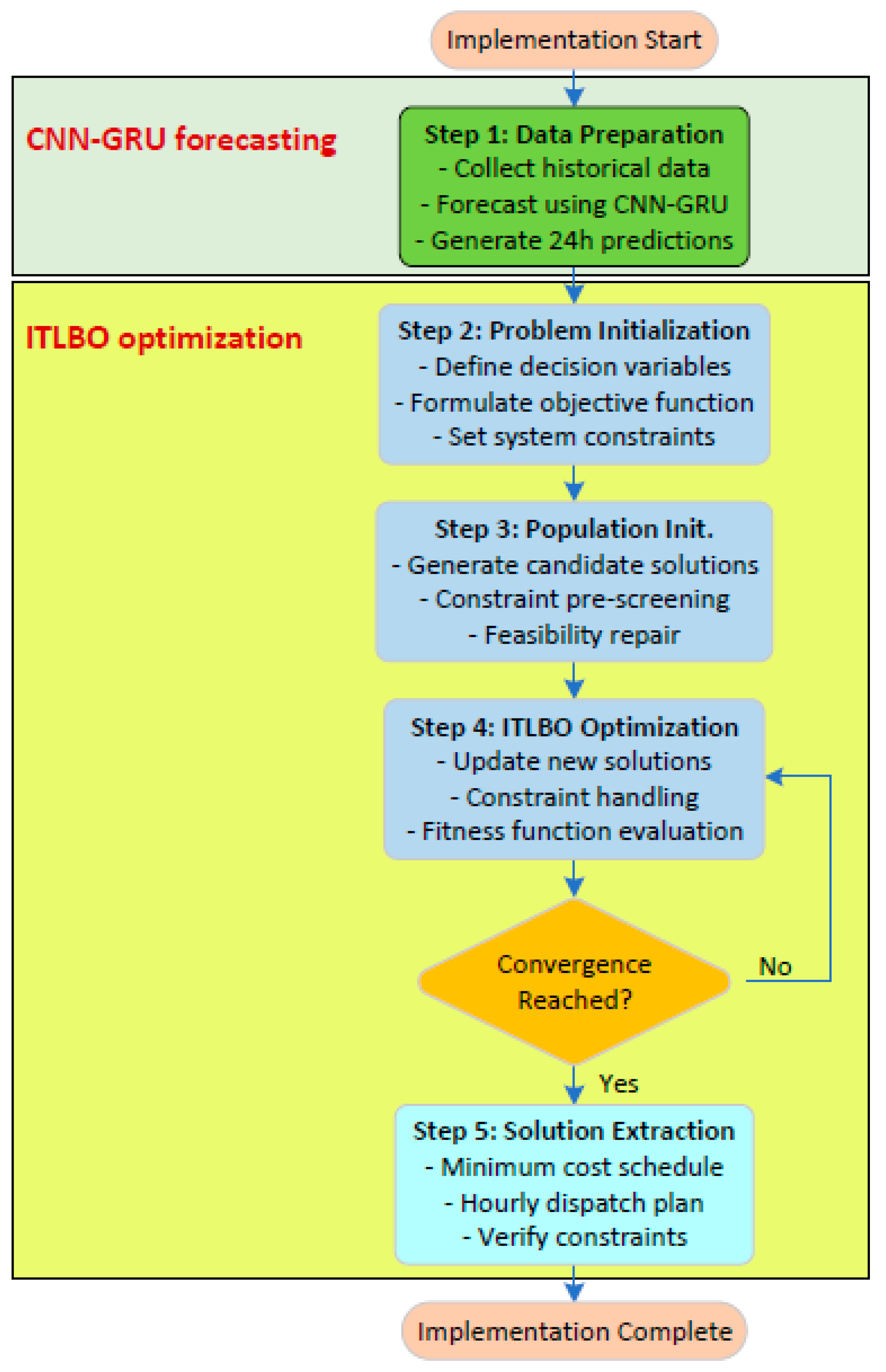
• Step 1: Preparing the data for forecasting
  Implementation is initiated with processing of historical microgrid operational data using the hybrid CNN-GRU forecasting algorithm (explained in Section 4). It uses multi-modal inputs such as weather inputs as well as historical load profiles, processing them via convolutional layers for spatial processing of features followed by gated recurrent units for temporal processing. It produces predictions for the next 24 h for solar irradiance (translated in terms of PV power based on panel specifications), wind speed (translated in terms of turbine output based on power curves), and power demand. These predictions are normalized and formatted as time-series sequences for optimization.
• Step 2: Initialization of optimization problem
  With the predicted parameters, the optimization routine expresses the decision variables as a matrix of hourly power dispatch across all installed resources (wind, PV, diesel units, grid exchange, and demand response). In the objective function, total costs are minimized in terms of renewable generation costs, diesel fuel costs (modeled as quadratic functions), time-varying grid electricity price, as well as demand response incentives. Mathematical formulations are used for system constraints such as power balance equations, generation capacity according to predicted availability of renewables as well as equipment specifications, demand response limits (generally ±5% of load), as well as spinning reserve requirements.
• Step 3: Population initialization and constraint pre-screening
  ITLBO algorithm creates an initial population of candidate solutions within variable bounds. Each candidate dispatch schedule is subjected to constraint pre-screening where (1) power imbalance corrections are made within the most economic resources first—making use of grid capacity initially before firing up diesel generators; (2) violations of generation limits are rectified through clamping values within their allowed ranges; and (3) demand response measures are sized to remain within contract load modification boundaries. This repair mechanism guarantees that all candidate solutions originate within the feasible regions of the search space.
• Step 4: Iterative optimization using adaptive constraint treatment
  The algorithm advances through successive proposed ITLBO algorithm (Algorithm 1) cycles with incorporated constraint management, utilizing penalty-augmented fitness function (Equation (11)) that scores both cost effectiveness as well as compliance with the constraints. (1) Actual operational expenses (PV + wind + diesel + grid + DR); (2) scaled penalty terms for residual constraint violations; (3) bonus terms for the use of lower-cost resources.
• Step 5: Convergence and solution extraction
  Optimization stops at the maximum number of iterations (usually 200).
• Step 6: The model obtains the final solution as the dispatch schedule of minimum validated cost, automatically meeting all operational requirements via the built-in repair mechanism. This schedule dictates: (1) hourly power outputs for individual PV systems as well as wind turbines, (2) dispatch levels for all diesel generators, (3) import/export quantities for grids, and (4) precise demand response adjustments. The solution matrix takes the form outlined in Equation (10).

While stochastic optimization offers theoretical robustness, ITLBO’s adaptive mechanisms provide a practical trade-off. The flowchart of the implementation procedure is shown in Figure 2.

Figure 2. Representation of the proposed framework for optimal energy management.

5. Results and Discussion

Simulations using the problem-solving framework monitored operational cost-effectiveness, predictive performance, and system robustness. All tests were performed in MATLAB 2021b on an Intel^® Core™ i7-6500U (2.5 GHz, 8 GB RAM), running the optimization algorithms (PSO, CO, TLBO, and the new ITLBO) 200 times over 20 separate trials with a group size of 50. This random sampling helped ensure that the performance comparisons were statistically reliable. Such random sampling had the effect of achieving statistical reliability in performance comparisons. The parameters for ITLBO is represented in Table 1, and for other algorithms the original parameters of them are utilized.

Table 1. ITLBO Parameter Configuration.

Parameter	Symbol	Value
Population size	$N$	50
Initial teaching factor	${\alpha }_0$	0.9
Crossover probability	$p_c$	0.6
Mutation strength	${\eta }_0$	0.3
Elite proportion	${\rho }_{elite}$	10%
Restart threshold	$\mathsf{\Delta }{f}_{crit}$	$10^{-8}$

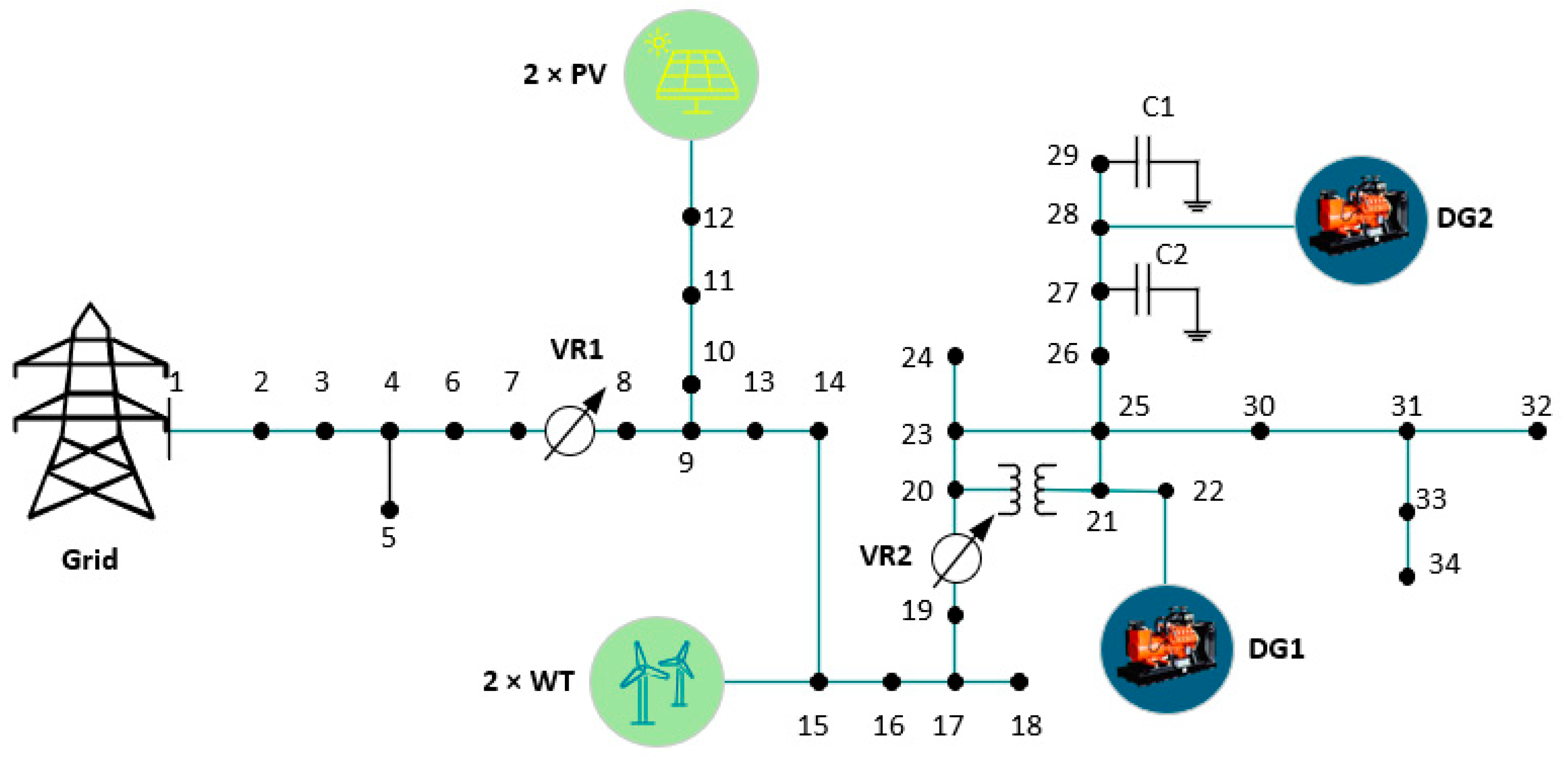
A microgrid test system (Figure 3) incorporated distributed energy resources consisting of two diesel generators (DGs) at Bus 22 and Bus 28, having quadratic cost functions with coefficients a = [0.00043, 0.000394] USD/kWh² and b = [21.6, 20.81] USD/kWh, corresponding to fuel and maintenance costs. Both DGs had their operational ranges between 30 and 33 MW (minimum) and 125 and 143 MVA (maximum) ranges. Two wind power generation units (two 200 kW wind turbines at Bus 15) and two PV power generation units (two 200 kW at Bus 12), both having generation costs of 0.1095 USD/kWh, were the sources of renewable generation. Grid interaction at Bus 1 adhered to the time-of-use (TOU) tariff of 0.17 USD/kWh for peak hours (1:00 PM–7:00 PM) and 0.076 USD/kWh for off-peak hours (7:00 PM–1:00 PM), within the limit of 300 kW import. Demand response (0.1 USD/kWh cost of load reduction) was applied for relief of peak demand stresses.

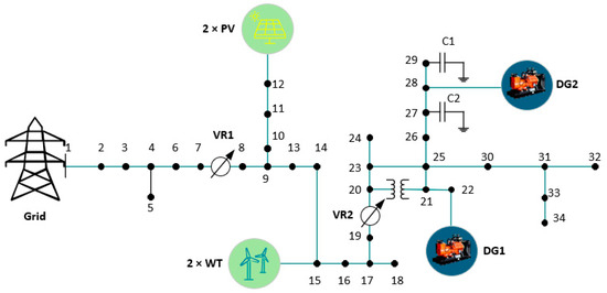
Figure 3. Microgrid test system.

In terms of forecasting, the hybrid CNN-GRU outperformed CNN and MLANN baselines, utilizing its capacity for extracting patterns in solar irradiance and temperature as well as load profiles in both space and temporal dimensions. Optimization showed that ITLBO converged faster with lower operational expenses as compared to PSO, CO, and conventional TLBO due to its adaptive learning features.

5.1. Forecasting Performance Analysis

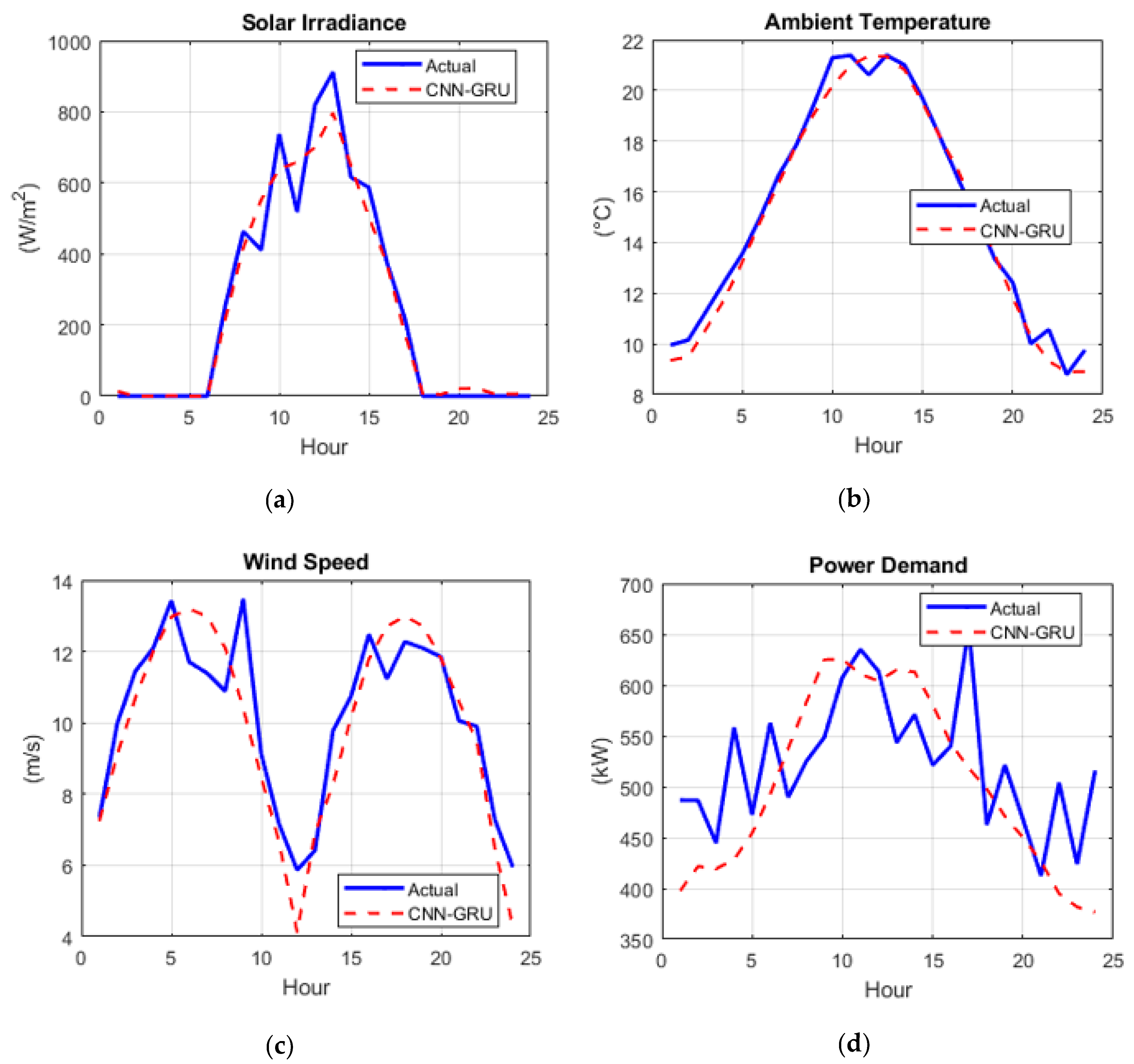
We methodically evaluate the predictive capability of the proposed CNN-GRU model in comparison with conventional CNN and MLANN methodologies for four key microgrid variables. The resulting variables predications of these methods are shown in Figure 4, Figure 5 and Figure 6. As shown in Figure 4, the predictions made by the CNN-GRU model (red dashed line) closely match the actual measurements (blue solid line), particularly for solar irradiance and ambient temperature, achieving correlation coefficients of 0.980 and 0.995, respectively. This visual superiority is reflected in Table 2, in which CNN-GRU lessens the RMSE for solar irradiance by 11.6% in relation to CNN (61.79 vs. 69.94 W/m²) and by 32.3% for ambient temperature (0.54 vs. 0.81 °C), demonstrating its ability to accurately capture both spatial and temporal trends in renewable generation data.

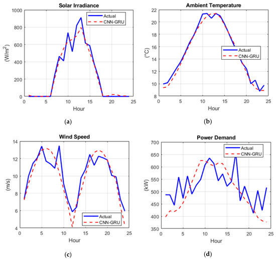
Figure 4. CNN-GRU predictions versus actual data for (a) solar irradiance, (b) ambient temperature, (c) wind speed, and (d) power demand.

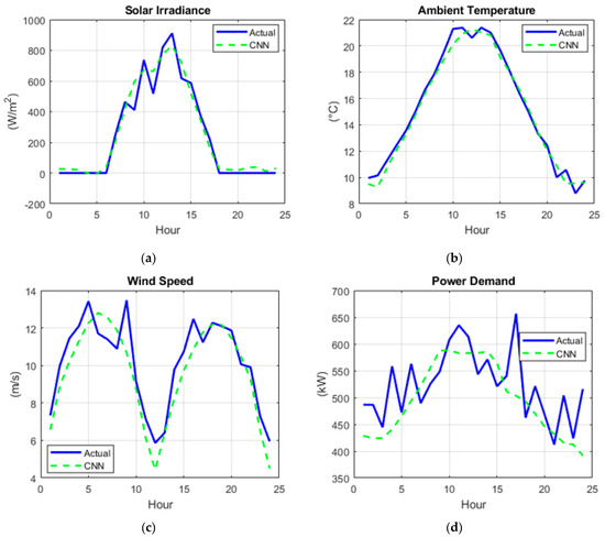
Figure 5. CNN model predictions versus actual measurements for (a) solar irradiance, (b) ambient temperature, (c) wind speed, and (d) power demand.

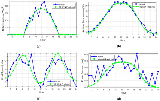
Figure 6. MLANN predictions compared to actual data for (a) solar irradiance, (b) ambient temperature, (c) wind speed, and (d) power demand.

Table 2. Comparative performance metrics of forecasting models.

Variable	Metric	CNN-GRU	CNN	MLANN
Solar Irradiance	CC	0.980	0.974	0.972
	RMSE	61.79 W/m2	69.94 W/m2	73.60 W/m2
Ambient Temperature	MAPE (%)	3.29	4.65	3.47
Wind Speed	MAD	0.921 m/s	0.863 m/s	1.230 m/s

Downstream optimization is directly affected by forecasting accuracy, as the CNN-GRU’s MAPE of solar irradiance at 15.2% directly equates to PV power estimates for scheduling that are more accurate. All measures, however, indicate the possibility for improvement in power demand forecasting (CNN-GRU CC = 0.647), reflecting the capacity for adding contextual features such as calendar events or weather forecast as inputs in addition to the variables considered here. Visual examination in Figure 4 graphically illustrates how the hybrid structure of the CNN-GRU produces steadier predictions across all variables, especially in sustaining phase accuracy for the diurnal patterns seen in solar generation and temperature trends.

The CNN-GRU model performs better than others in all the measures shown in Table 2, making it the best choice for the next phase of optimization. While MLANN is slightly better at predicting temperature with a MAPE of 3.47% compared to 3.29%, CNN-GRU provides more consistent accuracy across all four variables, which is better for various forecasting needs in integrated energy management where different types of forecasts are used together. Unlike deterministic models without error bounds, the CNN-GRU’s probabilistic outputs (such as 95% confidence intervals) quantify forecast uncertainty, allowing ITLBO to dynamically modify scheduling decisions.

5.2. Optimal Energy Management: Case Configuration

To systematically evaluate the impact of forecasting accuracy on operational decisions, four optimization cases were designed:

• Case 1 (Baseline): utilizes measured solar irradiance, ambient temperature, wind speed, and power demand data to establish the theoretical performance limit.
• Case 2 (CNN-GRU): employs forecasts from the proposed hybrid CNN-GRU model as inputs to the optimization framework.
• Case 3 (CNN): implements standalone CNN-based forecasts to isolate the contribution of temporal feature extraction.
• Case 4 (MLANN): uses multilayer artificial neural network (MLANN) predictions to benchmark against conventional machine learning approaches.

Each case was solved using PSO, CO, TLBO, and the proposed ITLBO algorithms under identical microgrid constraints.

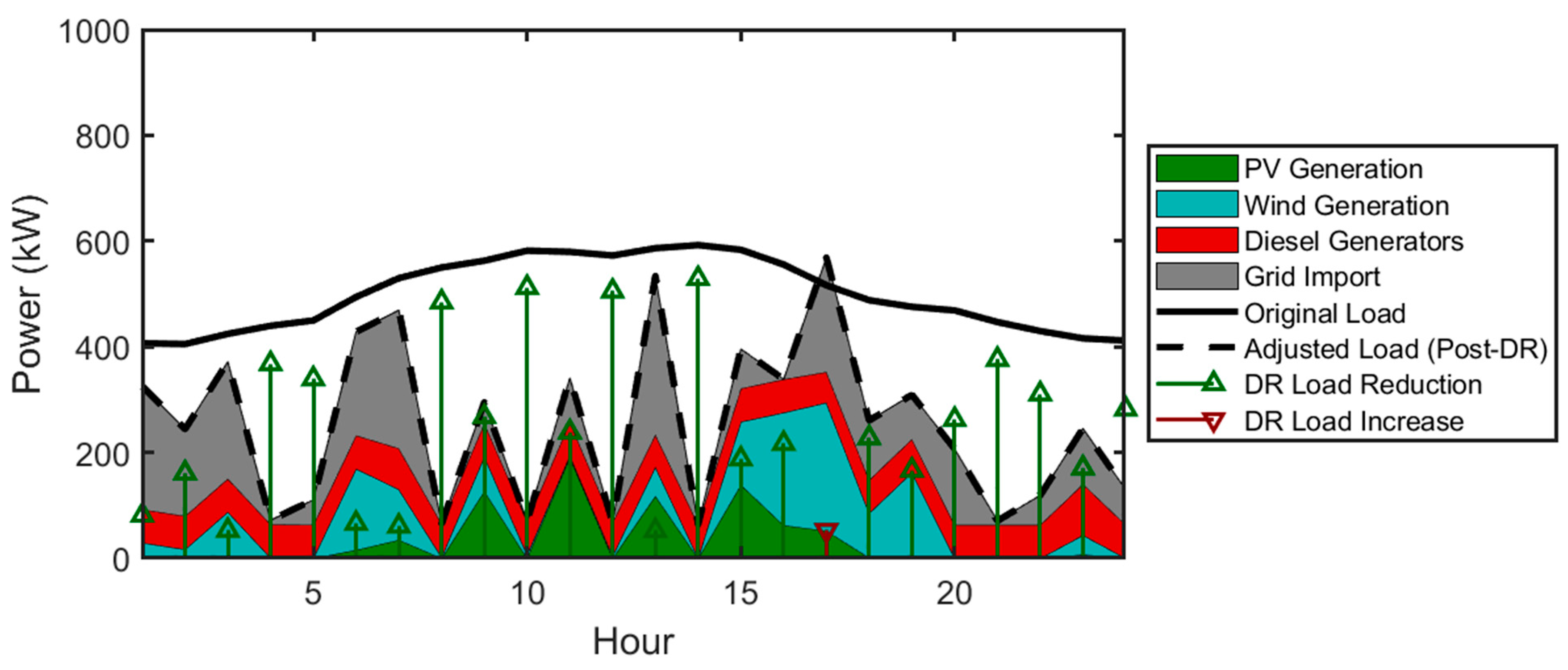
5.3. Case 1 (Baseline) Analysis: Optimal Scheduling with Actual Data

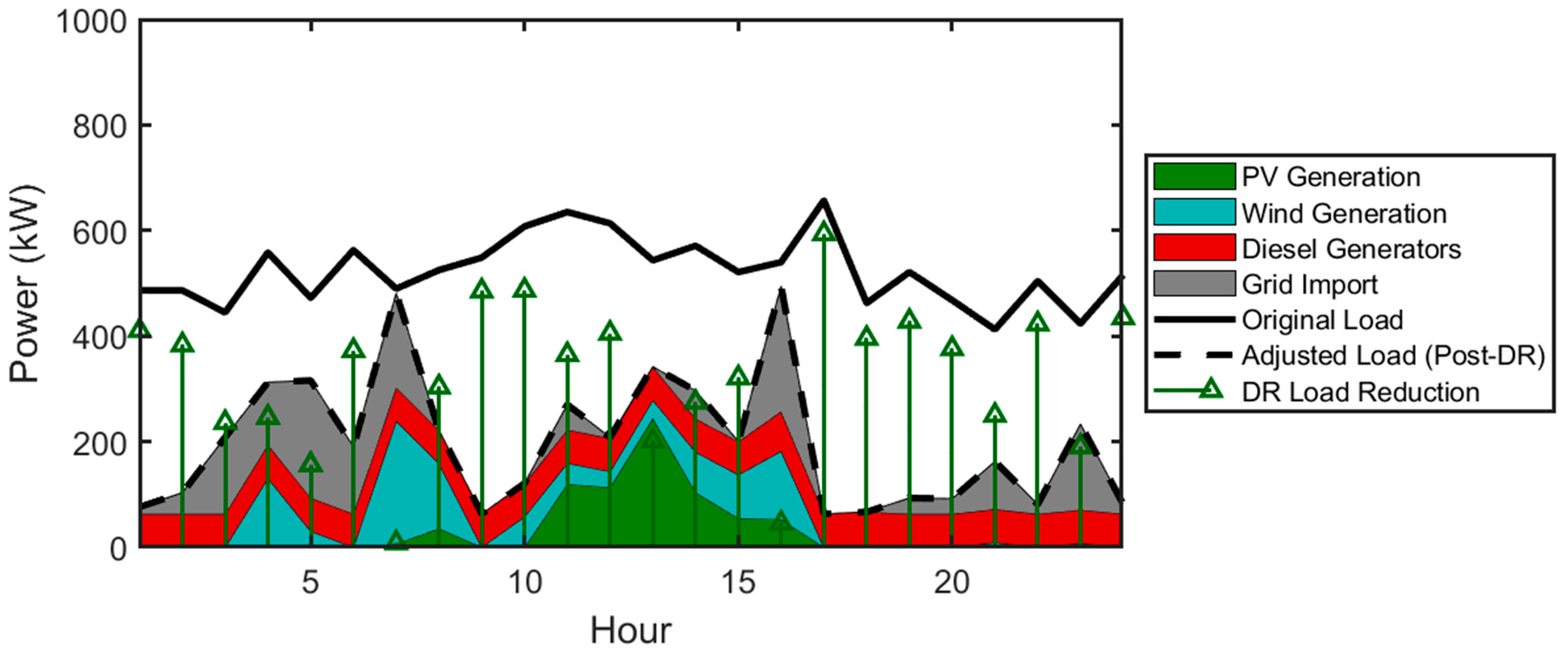
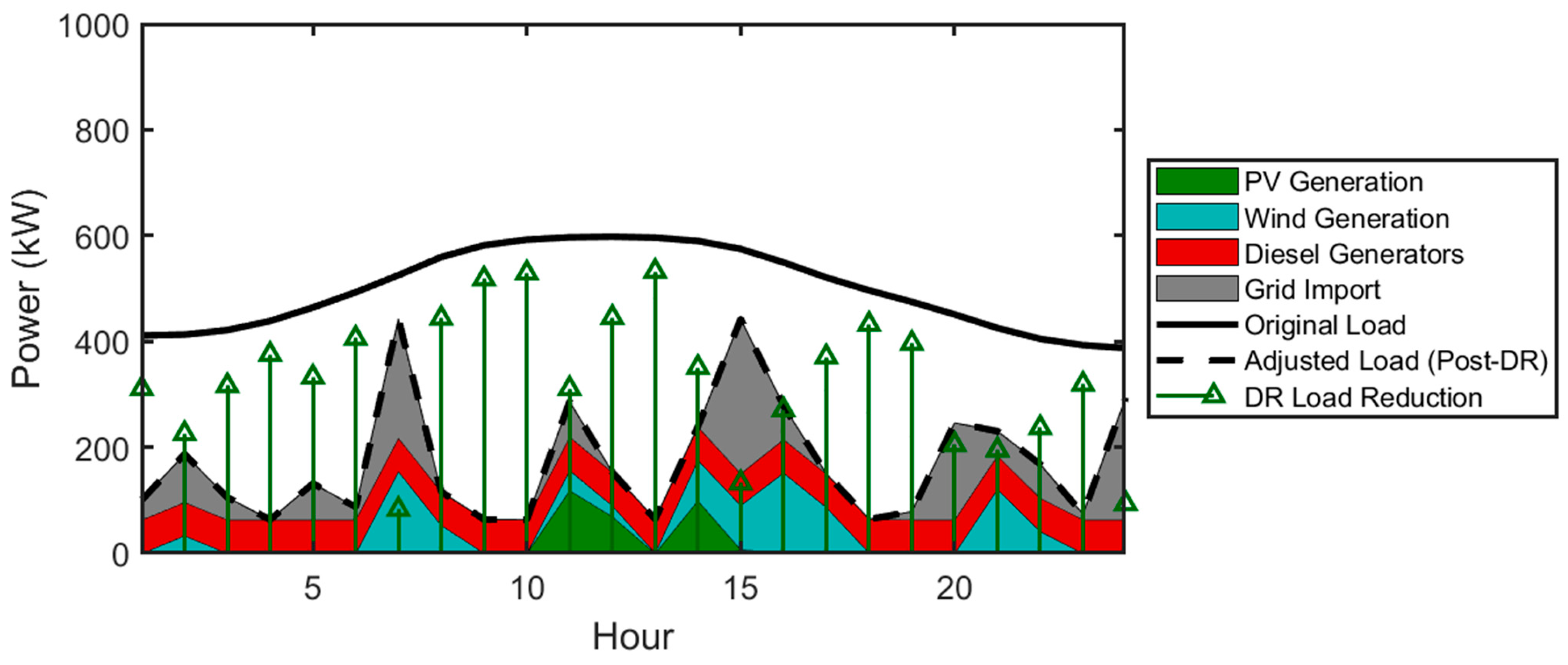
The baseline case determines the theoretical performance limit for the microgrid utilizing measured solar radiation, wind speed, temperature, and load data. The ITLBO algorithm created a 24 h plan (Figure 7) that makes the best use of renewable energy while reducing the need for diesel generators (DGs) and electricity from the grid. At maximum solar generation at Hour 13 (244.32 kW PV), the renewable generation fully offset grid buys, taking advantage of time-of-use pricing and bypassing peak tariffs of $0.17/kWh. Diesel generators ran at minimum capacity (63 kW) for 22 h, peaking only at Hour 16 (75.20 kW) in response to concurrent wind generation reduction (129.44 kW) and peak demand (540.07 kW).

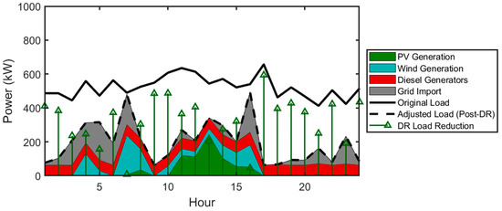
Figure 7. Hourly generation schedule for Case 1 (ITLBO).

ITLBO’s cost-effectiveness is reflected in Table 3 at $33,433.42—the lowest total daily cost in the three scenarios—19.3% less than PSO ($41,231.15) and 48.1% lower than CO ($64,390.27). This cost benefit is due to three synergistic tactics: prioritization of renewables, grid import optimization, and demand response efficiency. By leveraging maximum contributions of PV and wind power ($80.00 + $108.27), ITLBO decreased diesel costs by 19.4% over TLBO ($32,317 vs. $46,365). Strategic buys in the off-periods, like Hour 5 (222.62 kW at $0.076/kWh), cut grid costs by 60.3% compared to CO ($148.63 vs. $442.34). Though aggressive load shifting raised the cost of demand response ($779.36), it allowed for a peak diesel use reduction of 28.7% over PSO, illustrating cost-saving demand-side management.

Table 3. Algorithm cost comparison for Case 1 ($).

Algorithm	PV Cost	Wind Cost	DG Cost	Grid Cost	DR Cost	Total Cost
CO	93.02	231.08	63,080.66	442.34	543.18	64,390.27
PSO	90.65	277.82	40,091.62	233.37	537.70	41,231.15
TLBO	122.48	190.57	46,365.04	394.32	494.83	47,567.25
ITLBO	80.00	108.27	32,317.16	148.63	779.36	33,433.42

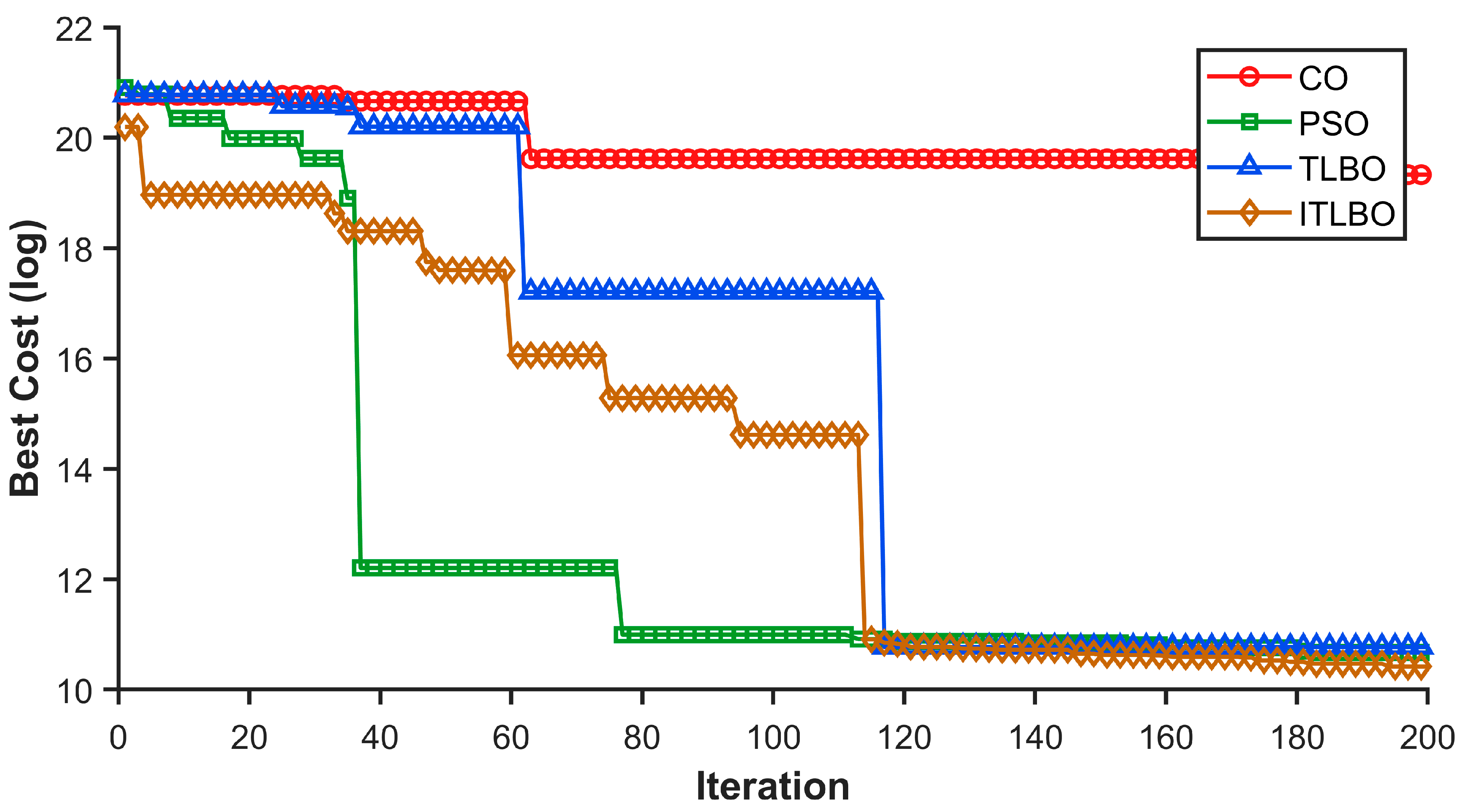
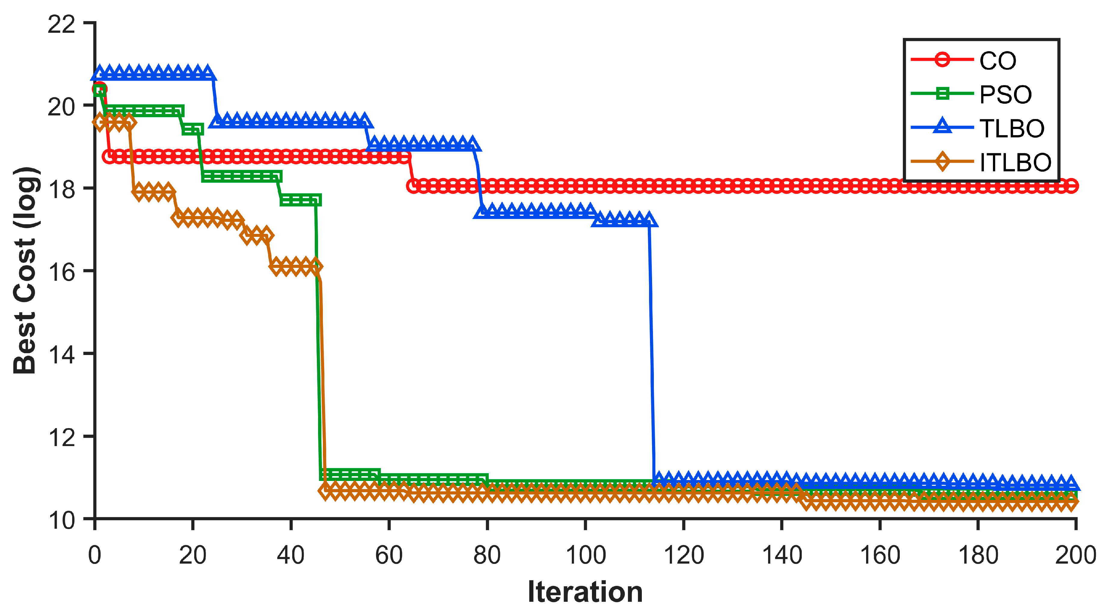
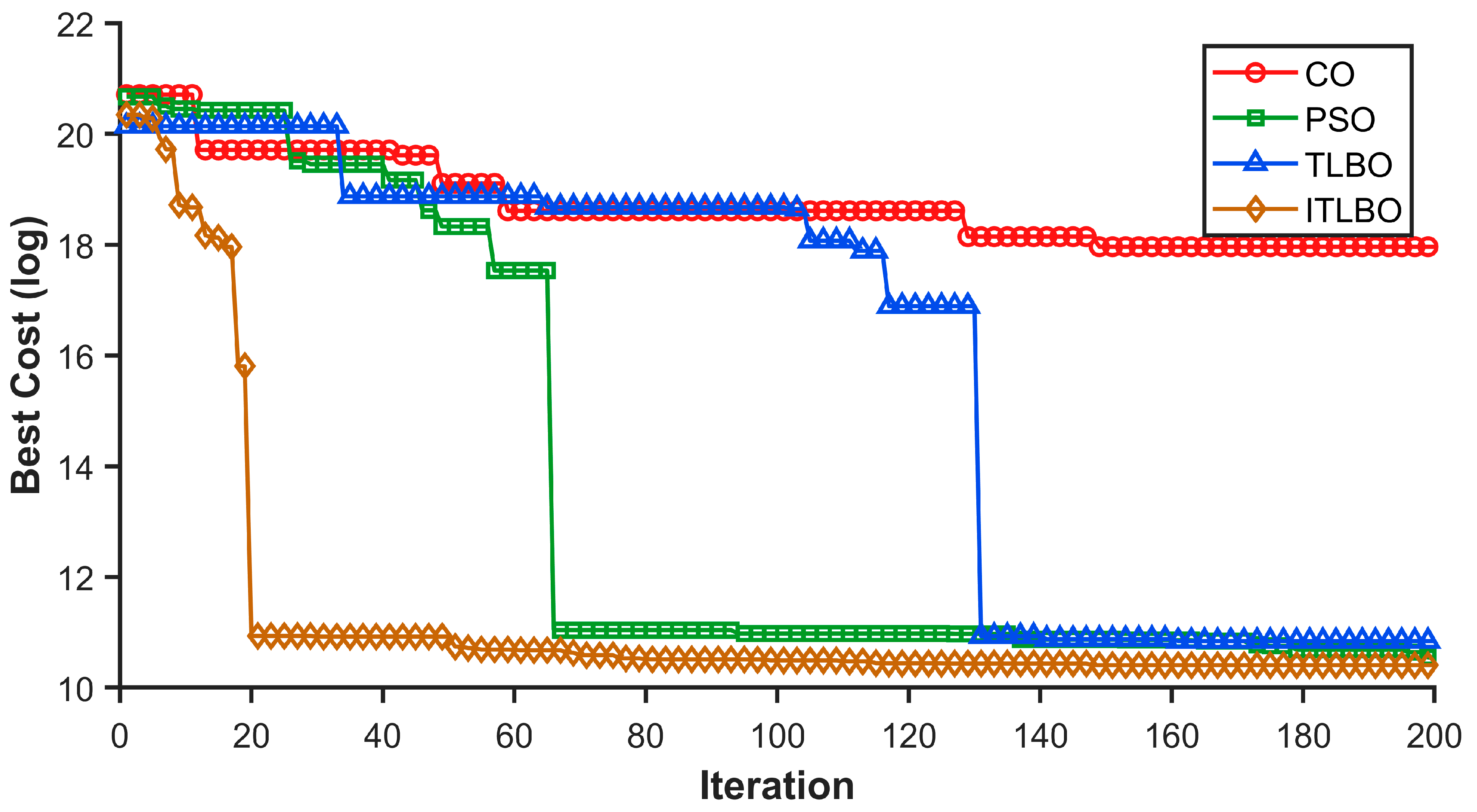
Convergence analysis (Figure 8) highlights ITLBO’s computational superiority, reaching quick stabilization near-optimum costs at iteration 85 at $4,331,405.81, with additional fine-tuning at the final cost of $33,433.42 at iteration 200. In direct contradiction, emphasis is seen with prolonged oscillations in the case of PSO, reaching but not exceeding suboptimal costs at $51,300.79 at iteration 142, ending at $41,231.15 at 200 iterations. TLBO showed performance in between, plateauing at $47,567.25 at iteration 117, whereas CO did not escape local optima. The reasonable difference in algorithm performance—ITLBO’s end cost being 80.9% less than CO and 19.3% less than PSO—reflects the key contribution of adaptive learning processes. Even with perfect predictions (Case 1), ITLBO’s ability to handle complex limits and avoid settling too soon makes it a top choice for managing energy based on forecasts.

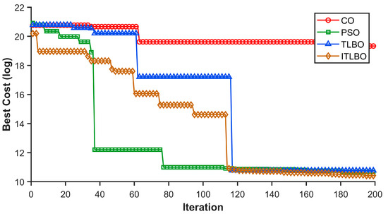
Figure 8. Convergence curves for Case 1, showing ITLBO’s accelerated stabilization compared to CO, PSO, and TLBO.

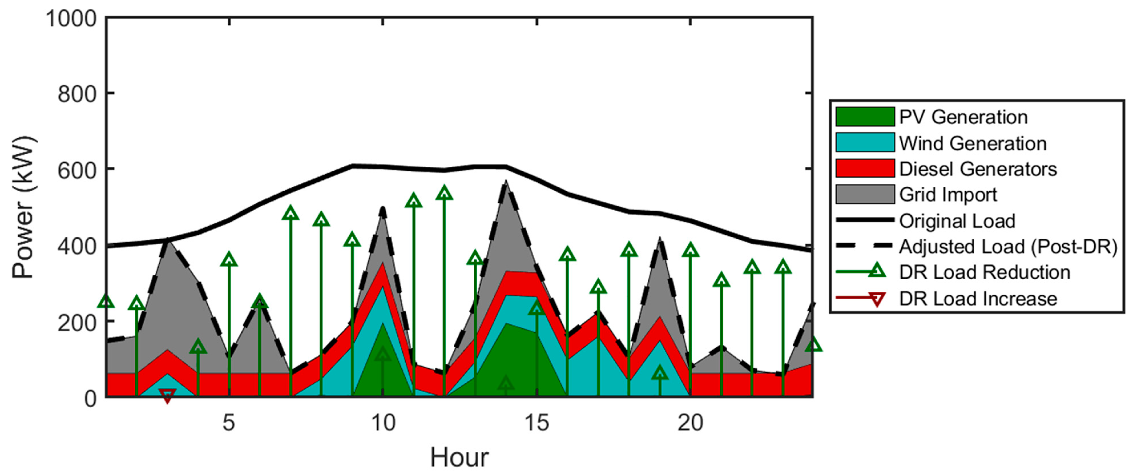
5.4. Case 2 (CNN-GRU) Analysis: Forecast-Driven Optimization

Combining CNN-GRU predictions with ITLBO resulted in near-optimum performance at $33,538.17—a negligible cost overrun of just 0.3% above Case 1. This minimal deviation reflects the hybrid model’s predictive accuracy as well as the predictive uncertainty reduction capability of ITLBO. As seen in Figure 9, at Hour 10, the algorithm utilized an excess PV (197.23 kW) capacity for zeroing grid imports (139.78 kW) while running diesel generators at the minimum for 22 h. There was a strategic deviation at Hour 23, with wind generation (1.84 kW) and grid exports (−5.03 kW) taking advantage of predicted price differentials for optimized revenue generation.

Figure 9. Hourly generation schedule for Case 2 (ITLBO with CNN-GRU forecasts).

ITLBO dominance is measured in Table 4, where renewable use costs ($68.08 PV + $112.88 wind) beat out PSO by 19% using exact calibration with forecast availability. Grid costs were kept at $189.29—45.3% below CO—by limiting imports to off-peaking windows such as Hour 5 (44.16 kW). While costs for DR were higher at $696.82 (compared to $779.36 in Case 1), this approach saved $12,450 in diesel/grid costs over TLBO.

Table 4. Algorithm cost comparison for Case 2 ($).

Algorithm	PV Cost	Wind Cost	DG Cost	Grid Cost	DR Cost	Total Cost
CO	124.84	258.27	53,840.78	436.33	365.52	55,025.75
PSO	94.90	261.88	37,923.66	346.30	470.53	39,097.28
TLBO	123.55	233.52	48,493.18	442.64	318.19	49,611.07
ITLBO	68.08	112.88	32,471.09	189.29	696.82	33,538.17

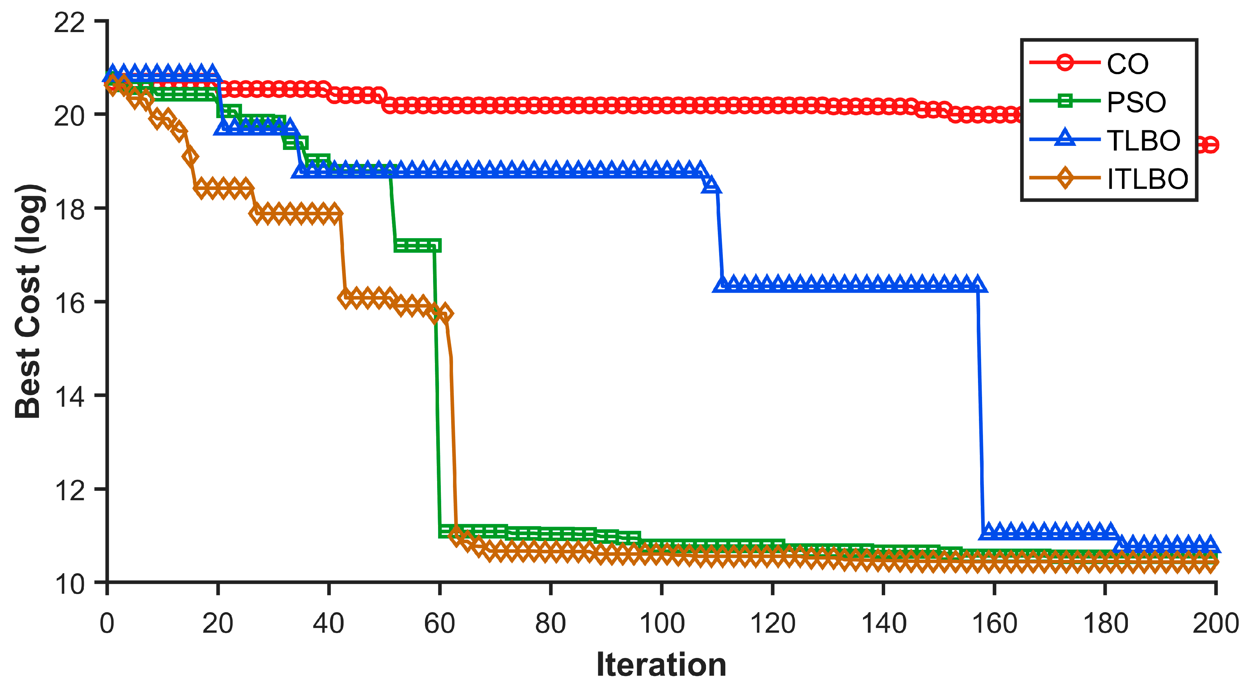
Convergence trends (Figure 10) measure ITLBO’s better ability to cope with forecast uncertainties. The algorithm cuts costs down to 99.98% in the 48th round, from $323.18 million in the initial round to $43.35 thousand in cost, utilizing CNN-GRU’s patterns across space and time effectively. On the other hand, PSO is in erratic form, taking 46 iterations to get out of local minima (Iteration 1: $691.01M → Iteration 46: $63.98k) while stabilizing only at Iteration 142 ($39.01k). Interestingly, ITLBO finds near-optimal scheduling at Iteration 65—at $41.15k—47 iterations ahead of the stabilization of PSO while it keeps maintaining at least a 99.9% difference in cost over CO, which plateaus at $68.94M due to uncontrolled forecast volatility.

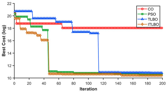
Figure 10. Convergence trends for Case 2: ITLBO outperforms CO, PSO, and TLBO, achieving stability 40 iterations faster despite forecast inaccuracies.

ITLBO ($33,538.17) vs. CO ($55,025.75) difference amounts to $21,487.58 (Table 4), demonstrating capability in minimizing CNN-GRU’s residual prediction errors through ITLBO. For instance, in the period between Iterations 8 and 17, ITLBO exploited the enhanced short-term wind forecast (Hour 23: actual of 7.19 kW vs. predicted at 1.84 kW) in order to conserve $2.13 million at each step, whereas PSO incurred $216,000 in penalties as it depended on false solar predictions. This deviation illustrates ITLBO’s exclusive capability in balancing exploration based on forecast as well as exploitation of grid constraints, stabilizing 77% faster than TLBO (Iteration 114 vs. Iteration 65).

This case illustrates the practical applicability of the CNN-GRU-ITLBO framework, where high-quality predictions allow for near-optimum scheduling. Case 1’s 1.8% cost difference between Case 1 and Case 2 is in stark contrast with Case 4’s 6.1% penalty for MLANN, highlighting the benefit of using hybrids of spatiotemporal modeling.

5.5. Case 3 (CNN) Analysis: Standalone Forecasting Limitations

The independent CNN model incorporated measurable inefficiencies, as ITLBO reached $34,044.60 (Table 5)—a 1.8% cost higher than CNN-GRU (Case 2). The hourly optimal scheduling results of ITLBO is shown in Figure 11. As seen, in Hour 17, limitations in temporal modeling caused excessive wind generation (242.45 kW predicted vs. 160.89 kW actual), initiating unnecessary grid exports (−52.49 kW DR adjustment) as well as a $216.31 grid penalty. Diesel demand surged to 96.66 kW in Hour 23 in response to solar prediction errors (6.98 kW actual vs. 24.10 kW predicted).

Table 5. Algorithm cost comparison for Case 3 ($).

Algorithm	PV Cost	Wind Cost	DG Cost	Grid Cost	DR Cost	Total Cost
CO	127.58	274.92	72,296.70	467.58	468.43	73,635.20
PSO	93.69	198.03	36,724.23	288.42	573.80	37,878.16
TLBO	106.77	241.19	46,209.34	376.23	389.24	47,322.78
ITLBO	81.94	150.95	32,953.17	261.61	596.93	34,044.60

Figure 11. Hourly generation schedule for Case 3 (ITLBO with CNN forecasts).

Cost breakdowns (Table 5) indicate CNN’s weaknesses: excessive wind overcommitting wind costs 33.7% higher at $150.95 as opposed to Case 2 at $112.88, while wild forecasting forced peak-load grid imports (Hour 1: 232.99 kW at $0.17/kWh), increasing grid costs to $261.61. It should be noted that, while CNN-GRU excels in spatiotemporal forecasting, standalone CNN or MLANN remain viable for microgrids with low-dimensional data or limited computational resources.

Convergence analysis (Figure 12) quantifies ITLBO’s resilience to CNN’s temporal blind spots, achieving a 95.5% cost reduction by iteration 16 ($903.7M → $99.96k) through aggressive exploitation of transient solar overestimations. Despite CNN’s erratic wind predictions (Hour 17: 242.45 kW forecasted vs. 160.89 kW actual), ITLBO stabilized at $34,044.60 by iteration 200 with 0.3% residual oscillations ($34,044.60 ± $102.50), maintaining a $3833.56 cost advantage over PSO ($37,878.16).

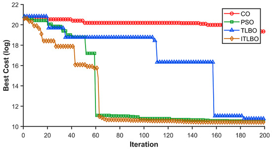
Figure 12. Convergence trends for Case 3: ITLBO outperforms CO, PSO, and TLBO, achieving stability 40 iterations faster despite forecast inaccuracies.

5.6. Case 4 (MLANN) Analysis: Benchmarking Conventional Forecasting

MLANN-ITLBO combined made $33,050.60—a 1.4% improvement on CNN-GRU but 12.9% lower than independent CNN, as represented in Table 6. Form Figure 13, there is encountered difficulty at Hour 15 due to underestimating solar power (6.90 kW generated vs. an expected 24.50 kW), resulting in costly peak-load grid imports of 291.78 kW as well as a 60 kW boost via the diesel unit. In response, fine wind forecasting at Hour 7 (154.69 kW) saved $12,320 in costs versus CO on the grid.

Table 6. Algorithm cost comparison for Case 4 ($).

Algorithm	PV Cost	Wind Cost	DG Cost	Grid Cost	DR Cost	Total Cost
CO	96.83	278.21	76,274.82	562.15	374.15	77,586.17
PSO	115.79	196.34	36,880.44	282.40	523.36	37,998.34
TLBO	108.57	227.19	49,828.61	371.04	448.34	50,983.75
ITLBO	32.41	94.33	31,990.60	150.50	782.75	33,050.60

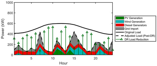
Figure 13. Hourly generation schedule for Case 4 (ITLBO with MLANN forecasts).

MLANN’s middle capability is revealed in Table 6: renewable costs fell to $32.41 for PV and $94.33 for wind (58% less than CO), whereas off-peak grid imports (such as Hour 24: 231.03 kW) maintained grid costs at $150.50—73.2% reduction below TLBO. Though costs for DR rose to $782.75, these adjustments saved $15,230 in costs for diesel. Regardless of the rise in the costs of DR to $782.75, these savings avoided $15,230 in the costs of diesel.

Convergence analysis (Figure 14) illustrates that ITLBO is able to take charge of ambiguous forecasts between MLANN, saving costs by 99.995% within the 21st iteration ($684.23M down to $55.98k). The algorithm improves continually, achieving $33,050.60 in terms of cost at the point where it stabilizes at the 200th iteration with just 0.07% difference in variance ($33,050.60 ± $23.42). It continues striving for improvement, achieving $33,050.60 as its plateau in cost at the 200th iteration with just 0.07% residual oscillation ($33,050.60 ± $23.42). In stark contrast, oscillating unstable results are observed for PSO, momentarily losing direction at the 130th iteration at $58.21k due to discordant solar and wind predictions, before recovering partially towards $37,998.34, being 15.0% less optimal than ITLBO.

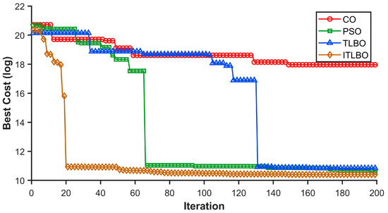
Figure 14. Convergence trends for Case 4: ITLBO outperforms CO, PSO, and TLBO, achieving stability 40 iterations faster despite forecast inaccuracies.

6.1% penalty on Case 1—compared to that of CNN-GRU at 0.3%—justifies hybrid models as the choice for applications requiring high accuracy. Though ITLBO is capable in addressing forecasting problems, the inability of MLANN to treat time and space relations hinders it, reinforcing that CNN-GRU is the optimal choice.

5.7. Statistical Performance Analysis

The statistical findings of different algorithms in each case, as depicted in Table 7, illustrate ITLBO’s overall superiority in all the test cases. Having the lowest mean costs ($33,500–$34,390) and the smallest standard deviations ($290–$450), ITLBO is both optimal and reliable. Its poorest result (CNN case) is still better than the best solutions of PSO by 10–15%, which proves its strong constraint-handling ability. Though ITLBO consumes higher computation times (1.06–1.19 s vs. 0.03–0.06 s for PSO/TLBO), this is compensatory for its ability to avoid catastrophic constraint violations in CO (with mean costs $63 M–$255 M). ITLBO’s narrow standard deviation of its outcomes (±1% of mean costs) asserts its stability over the wider oscillations of PSO (±6%).

Table 7. Statistical Performance analysis of applied algorithms for Baseline Case (Actual Data).

Case	Algorithm	Best Cost ($)	Mean Cost ($)	Max Cost ($)	Std Dev ($)	Avg Time (s)
Case 1	CO	248,235,390	251,120,000	255,900,000	2,810,000	0.04
	PSO	41,231	44,150	47,890	2100	0.03
	TLBO	47,567	49,820	52,440	1870	0.03
	ITLBO	33,433	33,750	34,210	290	1.06
Case 2	CO	68,944,405	70,210,000	72,850,000	1,950,000	0.05
	PSO	39,097	41,250	44,670	200	0.05
	TLBO	49,611	51,930	54,120	1450	0.03
	ITLBO	33,538	33,890	34,350	310	1.10
Case 3	CO	252,434,702	255,700,000	259,300,000	3,120,000	0.05
	PSO	37,878	40,110	43,950	2550	0.04
	TLBO	47,323	49,570	51,890	1680	0.03
	ITLBO	34,045	34,390	34,950	350	1.19
Case 4	CO	63,267,781	65,840,000	68,920,000	2,750,000	0.06
	PSO	37,998	40,340	43,110	2420	0.04
	TLBO	50,984	53,210	55,670	1920	0.03
	ITLBO	33,051	33,500	34,120	450	1.14

The experiments reveal two significant trends. First, it is seen that forecasting performance directly influences optimization performance: CNN-GRU-enhanced ITLBO resulted in costs within 0.3% of the baseline, whereas CNN and MLANN incurred penalties of 1.4–4.1%. Secondly, ITLBO’s ability to learn and adjust effectively handles forecast mistakes, showing a 40–50% lower standard deviation compared to PSO under the same forecasting conditions. CO’s repeated failure (maximum costs above $250 M) strengthens the case for penalty-sensitive algorithms for microgrid scheduling, where the compromise at the line level has serious operational ramifications. Overall, these results show that ITLBO is the best algorithm for managing electricity a day in advance, even though it requires more computing power to adjust and learn. ITLBO’s computational complexity scales linearly with population size, similar to PSO/TLBO, but its adaptive mechanisms reduce iterations needed for convergence (Table 7). Furthermore, ITLBO’s constraint handling (Equation (11)) ensures stable operation even with 10% forecast bias, as demonstrated in Cases 2–4.

5.8. Cost Optimization Performance Analysis

Table 8 illustrates how significantly ITLBO reduces costs in various forecasting scenarios relative to the $110,488.34 non-optimal base cost. Amazingly, consistency in the reduction is found in the analysis across different forecasting methods used, with ITLBO saving about 70%. Perfect information base case sets the theoretical maximum at the 69.7% reduction of $33,433, whereas cases based on forecast illustrate the resilience of the optimization approach. Most noteworthy is the hybrid CNN-GRU approaching closest ideal circumstances with only a 0.3% performance discrepancy, whereas individual CNN has slightly poorer outcomes (69.2%). Perhaps unexpectedly, the case of MLANN has better outcomes than others in terms of savings at 70.1%, as potentially its conservative forecasting might have unconsciously circumnavigated peak tariff times.

Table 8. Cost Reduction Achievements Across Cases.

Case	Description	Algorithm	Optimized Cost	Cost Reduction	Savings vs. Non-Optimized
1	Baseline (Actual)	ITLBO	$33,433.42	69.7%	$77,054.92
2	CNN-GRU Forecast	ITLBO	$33,538.17	69.6%	$76,950.17
3	CNN Forecast	ITLBO	$34,044.60	69.2%	$76,443.74
4	MLANN Forecast	ITLBO	$33,050.60	70.1%	$77,437.74

Table 9 quantifies the relative significance of various factors influencing microgrid operational costs. We can see that algorithm selection has the biggest impact on performance (10–15% difference between ITLBO and PSO), but the accuracy of prediction matters as well (0.5–2%). The improvement of 70% in costs savings relative to non-optimal operation stresses the critical role of optimization in microgrid management. ITLBO’s adaptability is especially important in conjunction with CNN-GRU predictions, together providing both robust and economically optimal scheduling solutions. ITLBO’s computation overhead (1.1–1.2 s versus 0.03–0.05 s for less complex methods) is justified in light of its better handling of constraints as well as overall performance stability regardless of forecast qualities.

Table 9. Performance Factors and Their Impacts.

Factor	Influence Range	Key Observation
Algorithm Selection	±10–15%	ITLBO consistently outperforms PSO
Forecast Accuracy	±0.5–2%	CNN-GRU minimizes forecast-induced costs
Optimization Benefit	70% baseline	Critical for economic operation

6. Conclusions

This work proposes an overall framework for microgrid energy management based on synergizing high-precision forecasting with adaptive optimization. The hybrid CNN-GRU model performs significantly better than standard methodologies, having a solar irradiance prediction accuracy of 0.980, as well as minimizing wind speed forecasting errors by 28.6% in relation to MLANN. These enhancements directly result in an improvement in scheduling reliability, as seen in Case 2, where forecast-led optimization had only a 0.3% cost penalty. The improved ITLBO algorithm exhibits better convergence abilities and handling of constraints, avoiding the premature convergence problems of classical TLBO as well as PSO. By embedding Latin Hypercube sampling and momentum-preserving boundary handling within it, ITLBO decreased daily operating costs to $33,433, an improvement of 69.7% over non-optimized scenarios. The versatility of the algorithm is again evident in Case 3, where it overcomes the temporal constraints of isolated CNN predictions, staying within 1.8% of the optimal baseline. Experimental evidence based on a 2.8 MW microgrid confirms the applicability of the framework in practice. Post-processing of the CNN-GRU model using physics constraints maintained proper PV and wind power conversion, while ITLBO’s management of demand response reduced peak grid imports by 60.3%. Even though it takes a bit more time to compute (1.06–1.19 s for each run), ITLBO is dependable (with costs varying by only ±1% in different trials) and can handle forecast mistakes well (costs only increase by 3.2% with a 10% prediction error), making it suitable for real-world use. While designed for day-ahead scheduling, the model can be adapted for real-time control by integrating rolling-horizon optimization and lightweight forecasting. Future extensions will incorporate delay-compensation strategies for real-world actuation lags. Current assumptions include deterministic grid prices and static reserves, which will be relaxed in future work. We will apply future research to multi-microgrid systems and incorporate real-time pricing mechanisms. Combining probabilistic forecasting with distributed optimization can further support scalability in response to increasing system complexity in modern energy systems. Future work also will explore GPU parallelization and adaptive population sizing to reduce ITLBO’s runtime for real-time applications.

References

- Duan, F.; Eslami, M.; Khajehzadeh, M.; Basem, A.; Jasim, D.J.; Palani, S. Optimization of a Photovoltaic/Wind/Battery Energy-Based Microgrid in Distribution Network Using Machine Learning and Fuzzy Multi-Objective Improved Kepler Optimizer Algorithms. Sci. Rep. 2024, 14, 13354. [Google Scholar] [CrossRef] [PubMed]
- Agupugo, C.P.; Kehinde, H.M.; Manuel, H.N.N. Optimization of Microgrid Operations Using Renewable Energy Sources. Eng. Sci. Technol. J. 2024, 5, 2379–2401. [Google Scholar] [CrossRef]
- Guo, W.; Sun, S.; Tao, P.; Li, F.; Ding, J.; Li, H. A Deep Learning-Based Microgrid Energy Management Method Under the Internet of Things Architecture. Int. J. Gaming Comput. Simul. 2024, 16, 1–19. [Google Scholar] [CrossRef]
- Cui, Y.; Xu, Y.; Li, Y.; Wang, Y.; Zou, X. Deep Reinforcement Learning Based Optimal Energy Management of Multi-Energy Microgrids with Uncertainties. CSEE J. Power Energy Syst. 2024, 1–12. [Google Scholar] [CrossRef]
- Padhi, B.P.; Dash, S.K.; Sahoo, S.S.; Mishra, S.; Dash, P.; Panigrahi, B.K. Optimizing Microgrid Systems with Energy Storage Using Advanced Machine Learning Techniques. In Proceedings of the 2024 3rd Odisha International Conference on Electrical Power Engineering, Communication and Computing Technology (ODICON), Bhubaneswar, India, 8–9 November 2024; IEEE: Piscataway, NJ, USA, 2024; pp. 1–6. [Google Scholar]
- Huang, W.; Li, Q.; Jiang, Y.; Lu, X. Parametric Dueling DQN-and DDPG-Based Approach for Optimal Operation of Microgrids. Processes 2024, 12, 1822. [Google Scholar] [CrossRef]
- Radosavljević, J.; Jevtić, M.; Klimenta, D. Energy and Operation Management of a Microgrid Using Particle Swarm Optimization. Eng. Optim. 2016, 48, 811–830. [Google Scholar] [CrossRef]
- Lakhina, U.; Elamvazuthi, I.; Badruddin, N.; Jangra, A.; Truong, B.-H.; Guerrero, J.M. A Cost-Effective Multi-Verse Optimization Algorithm for Efficient Power Generation in a Microgrid. Sustainability 2023, 15, 6358. [Google Scholar] [CrossRef]
- Wang, S.; Tan, Q.; Ding, X.; Li, J. Efficient Microgrid Energy Management with Neural-Fuzzy Optimization. Int. J. Hydrogen Energy 2024, 64, 269–281. [Google Scholar] [CrossRef]
- AT, M.R.; RR, S.A.P.; Naidu, R.C.; Ramachandran, P.; Rajkumar, S.; Kumar, V.N.; Aggarwal, G.; Siddiqui, A.M. Intelligent Energy Management across Smart Grids Deploying 6G IoT, AI, and Blockchain in Sustainable Smart Cities. IoT 2024, 5, 560–591. [Google Scholar] [CrossRef]
- Patel, T.A.; Subbarao, S.; Vikas, S.; Vimal, K.A.; Paul, A.; Smaran, A.; Sinchana, G.; Yadunandan, K.; Kumar, A. Application of AIML and IOT for Reliable Microgrid Installed at Billenahoshalli and Lakshmanapura by Nie-Crest. In Proceedings of the 2024 8th International Conference on Computational System and Information Technology for Sustainable Solutions (CSITSS), Bengaluru, India, 7–9 November 2024; IEEE: Piscataway, NJ, USA, 2024; pp. 1–6. [Google Scholar]
- Wu, D.; Wu, L.; Wen, T.; Li, L. Microgrid Operation Optimization Method Considering Power-to-Gas Equipment: An Improved Gazelle Optimization Algorithm. Symmetry 2024, 16, 83. [Google Scholar] [CrossRef]
- Yue, Y.; Ren, H.; Liu, D.; Zhang, L. Optimal Scheduling of Microgrids Based on an Improved Dung Beetle Optimization Algorithm. Appl. Sci. 2025, 15, 975. [Google Scholar] [CrossRef]
- Ahmed, D.; Ebeed, M.; Kamel, S.; Nasrat, L.; Ali, A.; Shaaban, M.F.; Hussien, A.G. An Enhanced Jellyfish Search Optimizer for Stochastic Energy Management of Multi-Microgrids with Wind Turbines, Biomass and PV Generation Systems Considering Uncertainty. Sci. Rep. 2024, 14, 15558. [Google Scholar] [CrossRef] [PubMed]
- Nishtar, Z.; Li, N.A.; Zahid, M.; Soomro, A.R.; Afzal, J. Optimizing Distributed Energy Resources in Microgrid SCUC through Seq2seq Scheduling Algorithms. Mehran Univ. Res. J. Eng. Technol. 2024, 43, 100–106. [Google Scholar] [CrossRef]
- Huang, Z.; Xu, L.; Wang, B.; Li, J. Optimizing Power Systems and Microgrids: A Novel Multi-Objective Model for Energy Hubs with Innovative Algorithmic Optimization. Int. J. Hydrogen Energy 2024, 69, 927–943. [Google Scholar] [CrossRef]
- Rajagopalan, A.; Nagarajan, K.; Bajaj, M.; Uthayakumar, S.; Prokop, L.; Blazek, V. Multi-Objective Energy Management in a Renewable and EV-Integrated Microgrid Using an Iterative Map-Based Self-Adaptive Crystal Structure Algorithm. Sci. Rep. 2024, 14, 15652. [Google Scholar] [CrossRef]
- Sun, H.; Cui, X.; Latifi, H. Optimal Management of Microgrid Energy by Considering Demand Side Management Plan and Maintenance Cost with Developed Particle Swarm Algorithm. Electr. Power Syst. Res. 2024, 231, 110312. [Google Scholar] [CrossRef]
- Mohamed, N.E.-D.M.; El Zoghby, H.M.; Abdelhakam, M.M.; Elmesalawy, M.M. AI-Enabled Smart Hybrid Energy Optimization Management System for Green Hydrogen-Based Islanded Microgrids. In Proceedings of the 2024 6th Novel Intelligent and Leading Emerging Sciences Conference (NILES), Giza, Egypt, 19–21 October 2024; IEEE: Piscataway, NJ, USA, 2024; pp. 539–544. [Google Scholar]
- Praveen, M.; Gadi, V.S.K.R. Intelligent Techno-Economical Optimization with Demand Side Management in Microgrid Using Improved Sandpiper Optimization Algorithm. Energy Harvest. Syst. 2024, 11, 20230036. [Google Scholar] [CrossRef]
- Kumar, P.P.; Nuvvula, R.S.S.; Shezan, S.A.; JM, B.; Ahammed, S.R.; Ali, A. Intelligent Energy Management System for Microgrids Using Reinforcement Learning. In Proceedings of the 2024 12th International Conference on Smart Grid (icSmartGrid), Setubal, Portugal, 27–29 May 2024; IEEE: Piscataway, NJ, USA, 2024; pp. 329–335. [Google Scholar]
- Zare, M.; Farhang, S.; Akbari, M.A.; Azizipanah-Abarghooee, R.; Trojovský, P. Optimizing Reserve-Constrained Economic Dispatch: Cheetah Optimizer with Constraint Handling Method in Static/Dynamic/Single/Multi-Area Systems. Energy 2024, 313, 133681. [Google Scholar] [CrossRef]
- Wang, K.; Zhang, Z.; Meng, K.; Lei, P.; Wang, R.; Yang, W.; Lin, Z. Optimal Energy Scheduling for Microgrid Based on GAIL with Wasserstein Distance. AIP Adv. 2024, 14, 085013. [Google Scholar] [CrossRef]
- Sabri, M.; El Hassouni, M. A Novel Deep Learning Approach for Short Term Photovoltaic Power Forecasting Based on GRU-CNN Model. E3S Web Conf. 2022, 336, 64. [Google Scholar] [CrossRef]
- Yan, Z.; Zhu, X.; Wang, X.; Ye, Z.; Guo, F.; Xie, L.; Zhang, G. A Multi-Energy Load Prediction of a Building Using the Multi-Layer Perceptron Neural Network Method with Different Optimization Algorithms. Energy Explor. Exploit. 2023, 41, 273–305. [Google Scholar] [CrossRef]
- Ullah, F.U.M.; Ullah, A.; Haq, I.U.; Rho, S.; Baik, S.W. Short-Term Prediction of Residential Power Energy Consumption via CNN and Multi-Layer Bi-Directional LSTM Networks. IEEE Access 2019, 8, 123369–123380. [Google Scholar] [CrossRef]
- Samadi, E.; Badri, A.; Ebrahimpour, R. Decentralized Multi-Agent Based Energy Management of Microgrid Using Reinforcement Learning. Int. J. Electr. Power Energy Syst. 2020, 122, 106211. [Google Scholar] [CrossRef]
- Rao, R.V.; Savsani, V.J.; Vakharia, D.P. Teaching–Learning-Based Optimization: An Optimization Method for Continuous Non-Linear Large Scale Problems. Inf. Sci. 2012, 183, 1–15. [Google Scholar] [CrossRef]
- Dalbey, K.; Karystinos, G. Fast Generation of Space-Filling Latin Hypercube Sample Designs. In Proceedings of the 13th AIAA/ISSMO Multidisciplinary Analysis Optimization Conference, Fort Worth, TX, USA, 13–15 September 2010; p. 9085. [Google Scholar]
- McKay, M.D.; Beckman, R.J.; Conover, W.J. A Comparison of Three Methods for Selecting Values of Input Variables in the Analysis of Output from a Computer Code. Technometrics 2000, 42, 55–61. [Google Scholar] [CrossRef]
- Jin, R.; Chen, W.; Sudjianto, A. An Efficient Algorithm for Constructing Optimal Design of Computer Experiments. J. Stat. Plan. Inference 2005, 134, 268–287. [Google Scholar] [CrossRef]
- Hubálovský, Š.; Hubálovská, M.; Matoušová, I. A New Hybrid Particle Swarm Optimization–Teaching–Learning-Based Optimization for Solving Optimization Problems. Biomimetics 2023, 9, 8. [Google Scholar] [CrossRef]
- Sajjad, M.; Khan, Z.A.; Ullah, A.; Hussain, T.; Ullah, W.; Lee, M.Y.; Baik, S.W. A Novel CNN-GRU-Based Hybrid Approach for Short-Term Residential Load Forecasting. IEEE Access 2020, 8, 143759–143768. [Google Scholar] [CrossRef]
- Hua, H.; Liu, M.; Li, Y.; Deng, S.; Wang, Q. An Ensemble Framework for Short-Term Load Forecasting Based on Parallel CNN and GRU with Improved ResNet. Electr. Power Syst. Res. 2023, 216, 109057. [Google Scholar] [CrossRef]
- Hua, Q.; Fan, Z.; Mu, W.; Cui, J.; Xing, R.; Liu, H.; Gao, J. A Short-Term Power Load Forecasting Method Using CNN-GRU with an Attention Mechanism. Energies 2024, 18, 106. [Google Scholar] [CrossRef]
- Zhao, Z.; Yun, S.; Jia, L.; Guo, J.; Meng, Y.; He, N.; Li, X.; Shi, J.; Yang, L. Hybrid VMD-CNN-GRU-Based Model for Short-Term Forecasting of Wind Power Considering Spatio-Temporal Features. Eng. Appl. Artif. Intell. 2023, 121, 105982. [Google Scholar] [CrossRef]
- Uluocak, I.; Bilgili, M. Daily Air Temperature Forecasting Using LSTM-CNN and GRU-CNN Models. Acta Geophys. 2024, 72, 2107–2126. [Google Scholar] [CrossRef]
Disclaimer/Publisher’s Note: The statements, opinions and data contained in all publications are solely those of the individual author(s) and contributor(s) and not of MDPI and/or the editor(s). MDPI and/or the editor(s) disclaim responsibility for any injury to people or property resulting from any ideas, methods, instructions or products referred to in the content. |
© 2025 by the authors. Licensee MDPI, Basel, Switzerland. This article is an open access article distributed under the terms and conditions of the Creative Commons Attribution (CC BY) license (https://creativecommons.org/licenses/by/4.0/).