Washout-Filter-Based Stabilization Control for Continuous Ethanol Fermentation Under Delay-Induced Product Inhibition

Abstract

Continuous ethanol fermentation is crucial for renewable bio-manufacturing, but delay-induced ethanol inhibition triggers self-oscillations via Hopf bifurcations, undermining productivity and stability. This study investigates instability mechanisms and proposes a washout-filter-aided control strategy. Using Hopf bifurcation theory, the critical delay time τ_c (20.97 h) was quantified, and it confirmed that τ > τ_c (intrinsic τ = 21.72 h) induces oscillations. Closed-loop analysis reveals that the filter extends τ_c to 25.57 h (e.g., K = 2, d = 0.5), expanding the stability margin by modulating ethanol dynamics through phase-shifted feedback. Numerical simulations and experimental validation demonstrate effective oscillation suppression, maintaining steady-state substrate (S* = 84.32 g/L), biomass (X* = 6.92 g/L), and ethanol (P* = 22.02 g/L) concentrations without sacrificing productivity. Unlike conventional methods, the strategy retains the system’s equilibrium structure, resists noise, and requires no additional hardware. This work bridges bifurcation analysis with practical control, offering a robust, scalable solution for industrial continuous ethanol production to mitigate delay-induced instabilities.

1. Introduction

Over the past decades, biological processes have emerged as a cornerstone of sustainable industrial production, offering renewable, low-carbon alternatives to traditional chemical synthesis for manufacturing commodities ranging from fuels to pharmaceuticals, and other commodities [1,2,3]. These processes encompass microbial fermentation for chemical production (e.g., alcoholic fermentation), biomass cultivation (e.g., baker’s yeast), metabolic extraction (e.g., carotene), and environmental remediation (e.g., wastewater treatment), all distinguished by their eco-friendliness and resource efficiency [4,5]. Despite these advantages, most bio-conversion processes remain batch-based [6,7], constrained by lengthy lag and stationary phases that limit productive time. For instance, Saccharomyces cerevisiae ethanol fermentation exhibits exponential growth for only 16–20% of a 60–72 h batch cycle, with inter-batch downtime for harvesting, cleaning, and sterilization further reducing productivity and elevates costs [8]. This has motivated the bioengineering community to pursue continuous fermentation technologies.

Continuous ethanol fermentation, while promising for its automation and round-the-clock operation, is plagued by a critical instability: self-sustained oscillations in substrate, biomass, and product concentrations under high ethanol stress [9,10,11]. As ethanol accumulates to inhibitory levels (50–80 g/L), S. cerevisiae metabolism is disrupted, forming a negative feedback loop that diminishes ethanol production, wastes substrate, and destabilizes reactor operation [12,13]. The core challenge lies in understanding the mechanisms driving these oscillations and developing robust control strategies to stabilize the process.

The delayed response of microorganisms to ethanol inhibition is central to these oscillatory dynamics. Early studies hypothesized that historical ethanol concentrations influence metabolic adjustments [14]. Li et al. [15] identified the rate of ethanol concentration increase as a key inhibitory factor, noting that high ethanol levels force microbes to reconfigure enzyme systems, introducing time lags in growth and substrate utilization. Jobses et al. [16] formalized this by modeling ethanol’s inhibition of intracellular metabolite synthesis (e.g., RNA/protein), creating a delay between substrate uptake and biomass production. Xiu et al. [17] further emphasized membrane transport delays for substrates and products, a framework later extended to link discrete time delays in inhibition terms with Hopf bifurcations and oscillatory behavior [18,19].

Existing strategies to mitigate oscillatory dynamics include operational adjustments (e.g., dilution rate tuning) [20,21] and in situ product removal via membrane separation [22]. However, these methods often require additional equipment or only prevent instability rather than address its root cause, limiting productivity gains. Bifurcation control [23] and feedback techniques, including PID [24], nonlinear [25], or model-based controllers [26], offer more targeted solutions, but their efficacy is constrained by model uncertainty, sensitivity to parameter variations, and the need for accurate state estimation, challenges that are particularly acute in biological systems characterized by noisy measurements and complex, time-varying interactions [27,28]. Therefore, a more mechanistic approach [10,29], explicitly accounting for delayed inhibition in controller design, is applied to yield robust, scalable solutions.

This study advances the state of the art by integrating Hopf bifurcation analysis with practical control engineering to develop a washout-filter-aided stabilization strategy tailored to delay-induced instabilities in continuous ethanol fermentation [30,31,32]. The paper is structured as follows: Section 2 formulates the fermentation model and analyzes stability, highlighting delay-induced Hopf bifurcations. Section 3 validates the model using experimental data and outlines the washout-filter design. Section 4 evaluates the control strategy through simulations and closed-loop analysis, and Section 5 concludes with insights into industrial implementation.

2. Preliminary

2.1. Model Description

A typical continuous fermentation model is predicated on two core assumptions: (1) the reactor operates with a constant volume, and its internal contents are uniformly mixed; (2) a single substrate-limited nutrient (e.g., glucose) is continuously fed into the reactor to support biomass/microorganism growth, while an equivalent volume of fermentation broth is simultaneously withdrawn as the product stream. Based on these premises, the mass balance equations for the substrate (S), biomass (X), and product (P) can be derived as follows:

$$\left\{\begin{array}{l}{\displaystyle \frac{dS}{dt}}=D(S_{in}-S)-\sigma X\\ {\displaystyle \frac{dX}{dt}}=-DX+\mu X\\ {\displaystyle \frac{dP}{dt}}=-DP+\rho X\\ S(0)=S_{in},X(0)=X_0,P(0)=P_0.\end{array}\right.$$

(1)

where D denotes the dilution rate, defined as the reciprocal of the reactor space-time; S_in represents the substrate inlet concentration; and σ, μ, and ε correspond to the specific substrate consumption rate, specific biomass growth rate, and specific product formation rate, respectively. Notably, for a given initial condition (S_in, X₀, P₀), the system is proven to be well-posed, and the existence and uniqueness of its solution can be verified via standard mathematical methods.

The complexity of System (1) stems from the sophistication of the kinetics governing microbial metabolism. Analogous to the Michaelis–Menten equation, the first widely recognized model describing biomass growth rate under single-substrate limitation was proposed by Monod. However, in S. cerevisiae fermentation, high ethanol concentrations exert an inhibitory effect on microbial metabolism, and thus the specific growth rate μ(S, P_τ) (where P denotes ethanol as the inhibitory product) can be expressed as follows [33]:

$$\begin{array}{l}\mu (S,P_{\tau })={\displaystyle \frac{{\mu }_{m}S}{S+K_s}}\cdot {\displaystyle \frac{K_i}{P_{\tau }+K_i}}\\ P_{\tau }:=P(t-\tau )\end{array}$$

(2)

where K_s is the half-saturation growth rate of the biomass, and K_i represents the inhibitory constant; P_τ refers to the time-delayed state of ethanol concentration, denoting that the inhibitory effect of ethanol on microbial metabolism manifests with a time lag of τ. Time delay, when regarded as a bifurcation parameter, has been reported to induce the emergence of limit cycles and Hopf bifurcations in such dynamic systems. However, prior to discussing the bifurcations induced by time delay, it is necessary to revisit the stability of the general system, particularly in the case of τ = 0 (i.e., the scenario without time delay), as this serves as the fundamental reference for analyzing delay-induced dynamic behaviors.

2.2. Stability Analysis for the System Without Delay

Considering τ = 0, equilibria of System (1) are obtained by setting the derivatives to zero, and output multiplicity is obtained. Apart from the washout solution (S_in, 0, 0), the second root gives the following:

$$D+{\displaystyle \frac{D{Y}_p{Y}_{xs}}{K_i}}(S_{in}-S^{*})={\displaystyle \frac{{\mu }_m{S}^{*}}{S^{*}+K_s}};X^{*}=(S_{in}-S^{*})Y_{xs};P^{*}=X^{*}{Y}_p$$

(3)

One can adopt the Hurwitz criterion for local stability analysis. When Equation (3) is substituted into (1), the characteristic equation is provided as follows:

$$(Y_{xs}\lambda +D)(D+\lambda -\mu )=0$$

(4)

From Equation (4), λ₁ = −D/Y_xs is non-negative, and local stability is determined by λ₂ = μ − D. Then, define D_c = μ_mS_in/(S_in + K_s), and the stability of the non-trivial root (Equation (3)) is assured when D_c > D. Similar conduct could be accomplished by substituting the washout solution (S_in, 0, 0) to System (1), and one can verify that for D_c < D, the equilibrium is stable. However, shifts between different equilibrium states might happen since the system encounters output multiplicity, i.e., for a given input D, multiple equilibria are generated. Hence, the global stability status is evaluated.

Assume the non-negative states Ω = {(S, X, P): ≥ 0} is an invariant and bounded set, which includes both the equilibria and (S_in, X₀, P₀). The following Lemma 1 provides that (1) is dissipative, and the proof is provided in Appendix A.

Lemma 1

(Dissipatedness [15]). All non-negative set Ω = {(S, X, P): ≥ 0} lies in the bounded set Ω eventually as time approaches infinite.

From Lemma 1, one can deduce that System (1) under the general specific growth kinetics (A − 1) is dissipative, indicating that unlimited duplication of biomass is not possible, and the system is bounded. This property is critical not only for the assessment of the stability status when τ = 0, but also for the oscillatory dynamics for τ ≠ 0.

The limiting subsystem gives the following:

$$\left\{\begin{array}{l}{\displaystyle \frac{dX}{dt}}=\left({\mu }_0\left(S_{in}-\rho /\sigma P\right)f(P)-D\right)X=\left(F_2(P)-D\right)X\\ {\displaystyle \frac{dP}{dt}}={\displaystyle \frac{\rho }{\mu }}{\mu }_0\left(S_{in}-\rho /\sigma P\right)f(P)X-DP=F_1(P)X-DP\end{array}\right.$$

(5)

where F_i(P) = μ(S_in − ρ/σP)f(P) for i = 1, 2. Further assuming that (X₀, P₀) are negligible small positive numbers at the beginning of the fermentation, then Equation (5) could reduce to the well-structured form, since F_i(0) = μ(S_in), F_i(ρ/σS_in) = 0 and F_i’(P) ≤ 0 if 0 ≤ P ≤ ρ/σS_in, and the vector form is as follows:

$$Y^{\prime }=F(Y),Y(0)=Y_0$$

(6)

when D_c = μ(S_in, P = 0) ≤ D, (0, 0) is the only equilibrium, and it is locally stable; and when D_c > D, (X*, P*) = (DF₂⁻¹(D)/F₁(F₂⁻¹(D)), F₂⁻¹(D)) is locally stable, and (0, 0) becomes unstable, the substitution of F(P) to System (11) gives the following:

$$\begin{array}{l}\nabla \cdot ({\displaystyle \frac{1}{X}}F)={\displaystyle \frac{\partial }{\partial X}}(F_1(P)-D)+{\displaystyle \frac{\partial }{\partial P}}(F_2(P)-{\displaystyle \frac{DP}{X}})\\ \hspace{1em}\hspace{1em}\hspace{1em}\hspace{0.33em}\hspace{0.33em}\hspace{0.17em}=F^{\prime }(P)-{\displaystyle \frac{D}{X}}<0\end{array}$$

(7)

By the Dulac’s criterion, the washout equilibrium (S_in, 0, 0) is globally stable when D_c < D; the nontrivial equilibrium (S*, X*, P*) is globally stable when D_c > D; and when D_c = D, both equilibria are coincident and a branch point is detected.

To avoid possible scenarios of the washout phenomenon [34], the stable property for the non-trivial solution (3) under the condition 0 < D < D_c is the necessary condition for subsequent analysis on delay-induced instabilities (i.e., τ ≠ 0) and stabilizing control.

2.3. Delay-Induced Hopf Bifurcation

If τ = 0, the solution (S*, X*, P*) in Equation (3) is stable if and only if all roots of the corresponding characteristic equation of the linearized equation have negative real parts, which is exhibited in Equation (4). Similar equivalence holds for differential-difference equations (i.e., τ ≠ 0), and the stability status is examined by the location of zeroes of the associated characteristic functions, only that the linearized delay differential equations are no longer ordinary polynomials, rather, they are exponential polynomials or quasi-polynomials.

Around (S*, X*, P*), the System (1) linearized provides the following form:

$$\begin{array}{l}x\prime \approx A(x-x^{*})+B(x_{\tau }-x^{*})\\ where:\\ {\left.A\right|}_{S^{*},X^{*},P^{*}}=\left(\begin{array}{ccc}-D-{\displaystyle \frac{X^{*}}{Yxs}}\cdot {\displaystyle \frac{\partial {\mu }^{*}}{\partial S}}& -{\displaystyle \frac{D}{Yxs}}& 0\\ X^{*}\cdot {\displaystyle \frac{\partial {\mu }^{*}}{\partial S}}& 0& 0\\ Y_p{X}^{*}\cdot {\displaystyle \frac{\partial {\mu }^{*}}{\partial S}}& D{Y}_p& -D\end{array}\right);{\left.B\right|}_{S^{*},X^{*},P^{*}}=\left(\begin{array}{ccc}0& 0& -{\displaystyle \frac{X^{*}}{Yxs}}\cdot {\displaystyle \frac{\partial {\mu }^{*}}{\partial P_{\tau }}}\\ 0& 0& X^{*}\cdot {\displaystyle \frac{\partial {\mu }^{*}}{\partial P_{\tau }}}\\ 0& 0& Y_p{X}^{*}\cdot {\displaystyle \frac{\partial {\mu }^{*}}{\partial P_{\tau }}}\end{array}\right)\end{array}$$

(8)

where x is the vector form that represents [S, X, P]^T. The characteristic equation gives the following:

$$\det (\lambda I-A-B{e}^{-\lambda \tau })=0$$

(9)

The roots of Equation (9) for the linearized system (8) give x(t) = e^λt, and the stability is determined by the sign of λ. The explicit expression is as follows:

$$\begin{array}{l}{(\lambda +D)}^2(\lambda +a+b{e}^{-\lambda \tau })=0\\ with:a={\displaystyle \frac{X^{*}}{Y_{xs}}}\cdot {\displaystyle \frac{\partial {\mu }^{*}}{\partial S}};b=-Y_p{X}^{*}{\displaystyle \frac{\partial {\mu }^{*}}{\partial P_{\tau }}}\end{array}$$

Other than the double roots λ = −D, the transcendental equation λ + a + be^−λτ = 0 is focused. Since a and b are positive, λ + a + be^−λτ is always positive for λ ≥ 0 when τ ≠ 0, indicating the transcendental equation has no real and non-negative root.

Heuristically, delay tends to destabilize. From the above analysis, τ = 0 obtains stable results for System (1), but unstable roots Re(λ) > 0 might emerge because of the transcendental in Equation (10), and varying τ might cause zeros of the characteristic Equation (9) to cross the imaginary axis, and System (1) might change stability status. By taking τ as a continuation parameter, one can examine the location of the roots and the direction of motion as they cross the imaginary axis. The following Lemma 2 is provided to make the discussion rigorous.

Lemma 2

[35]. Let L be a quasi-polynomial and τ > 0 is a constant delay time,

$$\begin{array}{ll}\hfill L(\lambda ,\tau )=& {\lambda }^n+a_1{\lambda }^{n-1}+\cdots +a_n{\lambda }^0+\hfill \\ & (b_1{\lambda }^{n-1}+b_2{\lambda }^{n-2}+\cdots +b_n{\lambda }^0)e^{-\lambda \tau }=0\end{array}$$

(10)

where ai and bi are real numbers. As τ is varying, the sum of the multiplicities of zeros of L on the open right-plane can change only if a zero appears on or across the imaginary axis.

From Lemma 2, one can infer that if Equation (9) presents a switch of stability status, a zero with positive real part can only occur when it crosses the imaginary axis. Hence, the conditions of the critical delay time τ_c could be obtained by substituting λ = iω into the transcendental equation, and the real and imaginary parts, when separated give,

$$\left.\begin{array}{l}a+b\cos (\omega \tau )=0\\ \omega -b\sin (\omega \tau )=0\end{array}\right\}\Rightarrow {\omega }^2=b^2-a^2$$

(11)

If b < a, the zero would not reach the imaginary axis, and a switch of stability will not happen, and System (1) remains asymptotically stable for any τ > 0. Instabilities of the delayed system are investigated by Skupin and Metzger [29], and the result is given in Theorem 1.

Theorem 1.

If D_b < D_c, it divides the domain D ∈ (0, D_c] into D₁ ∈ (0, D_b) and D₂ ∈ (D_b, D_c], the nontrivial condition (S*, X*, P*) of System (1) is asymptotically stable in D₁ for any τ > 0, and produces self-oscillatory outputs in D₂ when τ > τ_c > 0, where D_b is defined as,

$$\begin{array}{l}{D}_b=\mu \left(S_b,Y_p{Y}_{xs}(S_{in}-S_b)\right)={\displaystyle \frac{{\mu }_m{S}_b}{S_b+K_s}}\cdot {\displaystyle \frac{K_i}{Y_p{Y}_{xs}(S_{in}-S_b)+K_i}}\\ where\\ S_b=-K_s+K_s\sqrt{1+{\displaystyle \frac{K_i+Y_p{Y}_{xs}{S}_{in}}{K_s{Y}_p{Y}_{xs}}}}\end{array}$$

and τ_c is identified in Remark 1, and the proof is provided in Appendix B.

Remark 1.

To detect τ_c, Hopf bifurcation takes place when λ = iω is substituted into the transcendental equation, D ∈ (D_b, D_c] requires b > a, and the critical frequency gives,

$${\omega }_c=\sqrt{b^2-a^2}$$

(12)

so is τ_c,

$${\tau }_c={\displaystyle \frac{1}{{\omega }_c}}\arccos \left({\displaystyle \frac{a}{-b}}\right)+{\displaystyle \frac{2n\pi }{{\omega }_c}}$$

(13)

To mention, τ > τ_c > 0 is the necessary condition for the generation of oscillations, one needs to verify that delay destabilizes under condition D ∈ (D_b, D_c] and examine to satisfy,

$$sign\left\{\mathrm{Re}\left({\left.{\displaystyle \frac{d\lambda }{d\tau }}\right|}_{\lambda =i{\omega }_c}\right)\right\}>0$$

(14)

which promises the roots of the transcendental equation to cross the imaginary axis, and bifurcate out unstable eigenvalues, i.e., for any a τ > τ_c, a pair of conjugate roots λ_1,2 = α(τ) ± iω(τ) exists for the transcendental equation, where α(τ) > 0.

3. Materials and Methods

3.1. Dynamics of the Continuous Ethanol Fermentation Process

Based on the above analysis, it is now possible to investigate the oscillatory behavior of System (1). Both batch [36] and chemostat [37] experimental data are adopted to estimate parameters of the process. Firstly, the mass conservation relation is revealed by Y_xs and Y_p, which are obtained by the regression of batch data (with D = 0) under the guide of Equation (4), and the regression results are provided in Figure 1a,b. Then, MATLAB (Version 2018b) ode45 subroutine is adopted to predict the dynamics of System (1), where kinetic parameters μ_m ∈ (0.2, 0.8), K_s ∈ (0.2, 2.5), and K_i ∈ (0.1, 5) are unknown parameters. The least square method (i.e., lsqnonlin subroutine) is adopted to estimate these parameters, and the fitting is shown in Figure 1c. Lastly, the oscillatory data of the chemostat is regressed to identify the delay time in Figure 1d. Table 1 is a compilation of all the process parameters analyzed by theories. It bears noting that the estimation is conducted with τ = 0 for the batch mode production.

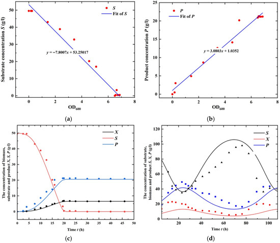
Figure 1. Experimental validation of the ethanol fermentation process. (a) Regression of Y_xs (1/7.800) by batch fermentation data of substrate content against OD600; (b) regression of Y_p (3.08) by batch fermentation data of product content against OD600, where the initial biomass is not zero, causing the curve to not necessarily intersect with the origin; (c) fitting of the kinetics of Equation (2) using batch fermentation data, where the delay of ethanol inhibition is not counted; (d) fitting of the oscillatory dynamics by varying the delay effect (τ = 21.72 h).

Table 1. Kinetics parameters used in the model.

Parameter	Description	Value
μm	Maximum specific biomass growth rate (h−1)	0.605
Yxs	Yield factor for substrate to biomass (g/g)	0.128
Yp	Yield factor for substrate to product (g/g)	3.08
Ks	Monod constant of saturation rate (g/L)	1.73
Ki	Inhibitory constant (g/L)	3.89
D/Din	Inlet substrate dilution rate (h−1)	—
Sin	Inlet substrate concentration (g/L)	—
S, X, P	Concentration of substrate, biomass, and product (g/L)	—
μ, σ, ρ	Specific growth rate of X, S, and P, respectively (h−1)	—
τc/τ	Critical-/intrinsic- delay time of product inhibition (h)	20.97/21.72

When the dilution rate is D = 0.089 h⁻¹ and input substrate concentration is S_in = 138 g/L, the nontrivial solution obtains S* = 84.32 g/L, X*= 6.92 g/L, and P* = 22.02 g/L. Since D < D_c = 0.5975 h⁻¹, the nontrivial equilibrium is stable when the inhibitory effect is uncounted (i.e., τ = 0). Adopting Equations (12) and (13), the critical delay time that might produce Hopf bifurcation is identified as τ_c = 20.97 h. Through Theorem 1, D > D_b = 0.03845 h⁻¹ indicates self-oscillatory behaviors are generated when τ > τ_c. To evaluate the direction of the Hopf bifurcations, when τ increases beyond τ_c, the eigenvalues cross the imaginary axis and a pair of complex conjugates λ_1,2 = α(τ) ± iω(τ) with α(τ) > 0 are obtained; moreover, from Lemma 1, the system with any τ ≠ 0 is dissipative, or non-divergent; hence, τ = τ_c undergoes super-critical Hopf bifurcation.

As shown in Figure 2, D_c and D_b curves separate the parameter space into three segments, and in between are domains that might produce self-oscillatory dynamics when the delay time τ > τ_c; the D_c curve separates out the washout condition, and low substrate content and high dilution rate might lead the bio-process to washout; the D_b curve is the stability line and the upper left segment causes the system to destabilize.

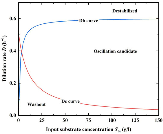
Figure 2. The D_c and D_b curves in the (S_in, D) domain separates out the parameter space that causes self-oscillatory dynamics to emerge for the ethanol fermentation process.

To obtain τ_c with varying D and S_in, Equation (13) is revisited. The calculation of a and b needs the equilibrium information (S*, X*, P*), which complicates the analytical expression of τ_c. Here, a stepwise method is proposed by using a symbol manipulation package Mathematica TM, where −a/b, arccos(−a/b), and τ_c are obtained consecutively. From Figure 3a, the series of lines approaches the D_c curve when −a/b → 1, leading to a quick decrease in ω_c to zero (Figure 3b). The contour in Figure 3c shows that varying D could lead to a more significant change in τ_c than that of S_in; increasing D causes the oscillatory behavior to emerge more easily, and τ_c presents a drastic change by approaching the D_c curve.

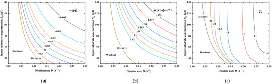
Figure 3. Critical delay time τ_c with varying D and S_in. (a) Calculation of −a/b; (b) Calculation of arccos(−a/b); (c) Calculation of τ_c.

The generation of self-oscillation is examined by numerical simulations, where, by arbitrarily setting D = 0.142 h⁻¹ and S_in = 35 g/L, it obtains τ_c = 20.97 h. Then, two points, τ = 23 h and τ = 20 h, are simulated and shown in Figure 4. For the stable one (τ = 21 h, Figure 4a), the system is attracted to three equilibria; whereas for the unstable one (τ = 23 h, Figure 4b), self-oscillations emerge. It bears noting that the increase in biomass content is in accordance with the increase in ethanol production as well as the decrease in residual substrate concentration, and the maxima of substrate consumption occur at the same time instants as the maxima of biomass and ethanol production. According to [24], the microorganism cells need time to adjust their enzyme system to accommodate high ethanol stress after the secretion of the product. Because of the delay response of microorganisms to the product, high ethanol content is accumulated. However, when the microorganisms begin to react with the high ethanol environment, biomass content undergoes a rapid decline, which then affects the secretion of the product and the living environment of the biomass. With a large amount of biomass under dormant conditions, the fermentation process is replaced by a high level of substrate, which is favorable for microorganism duplication and ethanol production, and provides an initial condition for the evolution to the next period of oscillations.

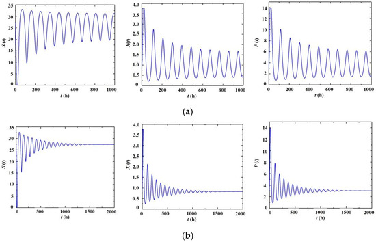
Figure 4. Time series of the continuous fermentation process for the dynamics of substrate (S), biomass (X), and product (P). (a) τ = 23 h and self-oscillations emerge. (b) τ = 20 h results in asymptotic stable outcomes.

It is known that delayed ethanol inhibition can give rise to eigenvalues with positive real parts. In the present work, we focus on Hopf bifurcations, which are non-linearizable [34]; specifically, normal-form analysis reveals that cubic terms constitute an integral component of the entire system. Notably, the stabilization strategy employing washout-filter-aided control enables the migration of dual unstable eigenvalues through the utilization of only a single washout filter.

In the following sections, continuous fermentation processes involving delayed ethanol inhibition are adopted as a case study, and the corresponding stabilization procedure is outlined as follows: (1) identify the causes underlying the formation of the unstable eigenspace and design the manipulated variables; (2) implement a washout filter to stabilize the unstable eigenvalues.

3.2. Stabilization Control for the Delayed System

In the previous study [33], instabilities (e.g., self-oscillation) originating from Hopf bifurcation causes the system to become un-linearizable, i.e., the original system and the linearized one possess different phase portraits. Stabilizing the delay-induced instability involves the elimination of unstable eigenvalues through feedback (also known as the bifurcation control). Hence, it is critical to first identify the unstable eigenspace.

From Equation (10), the transcendental equation λ + a + be^−λτ = 0 indicates that manifolds of the third equation in (1), which corresponds to the dynamics of P(t), produce the instabilities. Assuming the solution of λ + a + be^−λτ = 0 is a pair of complex conjugate roots λ_1,2 = α(τ) ± iω(τ) for τ > τ_c, then, the topologically equivalent manifold is provided in a small neighborhood τ ∈ (τ_c, τ_c+ε) for P(t), and by setting P(t) = x₁ + ix₂ and P(t)* = x₁ − ix₂, where i² = −1, one has,

$$\left\{\begin{array}{l}{x_1}^{\prime }=\alpha (\tau )x_1-\omega (\tau )x_2+O({\left|x\right|}^2)\\ {x_2}^{\prime }=\omega (\tau )x_1+\alpha (\tau )x_2+O({\left|x\right|}^2)\end{array}\right.$$

(15)

It bears noting that the higher-ordered terms in Equation (15) could be further processed, and the normal-form Hopf bifurcation is provided as follows,

$$\left(\begin{array}{c}{x_1}^{\prime }\\ {x_2}^{\prime }\end{array}\right)=\left(\begin{array}{cc}\alpha & -\omega \\ \omega & \alpha \end{array}\right)\left(\begin{array}{l}{x}_1\\ x_2\end{array}\right)\pm l_1(x_1^2+x_2^2)\left(\begin{array}{l}{x}_1\\ x_2\end{array}\right)$$

(16)

where l₁ is the first Lyapunov exponent, and when l₁ > 0 the system undergoes super-critical Hopf bifurcation, while l₁ < 0 is sub-critical.

Therefore, the oscillatory System (1) can be decomposed into stable and unstable manifolds. Intuitively, feedback control is most effectively applied to the unstable manifolds. When the oscillatory product concentration P(t) is adopted as the manipulated variable for the control input, the output signals, after processing by linear transfer functions (i.e., a washout filter), retain the same periodicity; this is proven in Lemma 3 below.

Lemma 3.

If a time-invariant system can be given in the form of a transfer function or one-to-one map, and the input u(t) is periodic with period T for t > 0, then, the output Nu approaches a steady state, also periodic with period T.

Proof. 

For a time-invariant system, if the input signal u(t) produces an output Nu(t), then, any time-shifted input u(t + Δ) results in a time-shifted output Nu(t + Δ). Let u_s be u extended periodically to t→∞, it becomes obvious that u(t) →u_s(t) as time approaches infinity, and if a final steady-state is obtained, one has Nu(t) →Nu_s(t) as time approaches infinity, and Nu_s(t) is periodic with period T,

$$N{u}_s(\cdot )(t+T)=N(u_s(\cdot +T))(t)=N{u}_s(t)$$

where the first equality is due to the time-variance of N and the second equality is due to the T-periodicity of u_s. □

Moreover, a washout filter could cause a delayed expression of the oscillatory dynamics by an auxiliary phase shift. Suppose the oscillating P(t) is approximated by a Fourier series,

$$\begin{array}{l}P(t)=a_0+{\displaystyle \sum _{n=1}^{\infty }\left(\sqrt{a_n^2+b_n^2}\sin [k\omega t+\phi (k)]\right)}\\ with:\phi (k)=\arctan \left({\displaystyle \frac{a_k}{b_k}}\right)a.e.in(0,T),\omega ={\displaystyle \frac{2\pi }{T}}\\ \left\{\begin{array}{l}{a}_k={\displaystyle \frac{1}{T}}{\displaystyle {\int }_{-\frac{T}{2}}^{\frac{T}{2}}P(t)\cos (kt)dt,n=0,1,2,\dots }\\ b_k={\displaystyle \frac{1}{T}}{\displaystyle {\int }_{-\frac{T}{2}}^{\frac{T}{2}}P(t)\sin (kt)dt,n=0,1,2,\dots }\end{array}\right.\end{array}$$

(17)

which, when passing through washout filter G(s) = s/(s + d), obtains the output y(t) as follows:

$$\begin{array}{l}y(t)=C_0{e}^{-dt}+{\displaystyle \sum _{k=1}^{\infty }k\omega \sqrt{(a_k^2+b_k^2)(k^2{\omega }^2+d^2)}\left(\sin [k\omega t+\phi (k)+{\phi }_1(k)]\right)}\\ with:{\phi }_1(k)=\arctan \left({\displaystyle \frac{d}{k\omega }}\right)\end{array}$$

(18)

where C₀ is related to the initial state, and when the washout filter constant d is positive (i.e., stable filter), y(t) converges to a zero-mean oscillation with shifted amplitude and phase shift angles φ₁(k), as compared with Equation (15), while preserving the same periodicity 2π/ω.

An accurate periodic feedback signal with a proper phase shift to gear well with the self-oscillating signal is essential for stabilizing control, but the oscillating trajectory of the dynamic system is very difficult to identify, while the mismatch between the internal oscillation and control inputs might cause resonance with even complicated dynamics. Concerning that the signal y(t) preserves oscillatory information 2π/ω, which, by fine-tuned feedback, could generate a delayed adjustment to eliminate the instabilities originating from the open-loop bifurcations.

Hence, leaving the stable manifolds unconsidered, the rigorous stabilization control reduces to the scale Equation (15). Without loss of generality, Equation (15) could be represented as follows,

$$x^{\prime }=Ax+Bu+h.o.t.$$

(19)

where the control u = [u₁, u₂]^T takes u = v + Ky, and k is the feedback gain, B is an arbitrary input-state transfer matrix. Adding the auxiliary state satisfies dz/dt = y, and the closed-loop system is provided as follows,

$$\left\{\begin{array}{l}{x}^{\prime }=Ax+Bu+h(x,u)\\ z^{\prime }=P(x-z)\\ u=K(x-z)\end{array}\right.$$

(20)

Stabilizing Equation (10) requires the following augmented matrix A_C to be Hurwitz, and the following Theorem 2 is provided; one can refer to Appendix C for the detailed proof.

$$\begin{array}{ll}\hfill \left(\begin{array}{c}{x}^{\prime }\\ z^{\prime }\end{array}\right)& =\left(\begin{array}{cc}A+BK& -BK\\ P& -P\end{array}\right)\left(\begin{array}{c}x\\ z\end{array}\right)\hfill \\ & =A_C\left(\begin{array}{c}x\\ z\end{array}\right)\end{array}$$

(21)

Theorem 2.

If A is non-singular and (A, B) is stabilizable, there exists (P, K) that makes A_C Hurwitz.

Based on the above analysis, one is able to design P based on the above perturbation theory. Consider only one washout filter is introduced to x_i with feedback u = K_jy,

$$\left\{\begin{array}{l}{x}^{\prime }=Ax+Bu+h.o.t.\\ z^{\prime }=x_i-dz=y\end{array}\right.\Rightarrow \left\{\begin{array}{l}{x}^{\prime }=\left(\begin{array}{cc}\alpha & -1\\ 1& \alpha \end{array}\right)\left(\begin{array}{l}{x}_1\\ x_2\end{array}\right)-(x_1^2+x_2^2)\left(\begin{array}{l}{x}_1\\ x_2\end{array}\right)+k_{j}y\\ y^{\prime }=f_i(x_i,k_{j}y)-dy\end{array}\right.$$

(22)

where y is the washout-filter output corresponding to x_i. Based on the Routh–Hurwitz stability criterion, one can obtain control gain K_j of the washout filter that stabilizes Equation (22), and the Jacobean of the augmented system gives,

$$\tilde{A}=\left[\begin{array}{cc}\left(\begin{array}{cc}\alpha & -1\\ 1& \alpha \end{array}\right)& {(BK)}_i\\ \begin{array}{cc}{\displaystyle \frac{\partial f_i}{\partial x_1}}& {\displaystyle \frac{\partial f_i}{\partial x_2}}\end{array}& {(BK)}_i-d\end{array}\right]$$

(23)

Expanding Equation (23) along the last column gives the characteristic polynomial P_c,

$$\begin{array}{ll}\hfill P_c& =\det (\tilde{A}-\lambda I_{2+1})\hfill \\ & =\left({(BK)}_i-d-\lambda \right)({\lambda }_{-i}-\lambda )+{\left({\displaystyle \frac{\partial f_i}{\partial x_1}}\right)}_n\cdot {(BK)}_i({\lambda }_{-i}-\lambda )\\ & =\left[\left({(BK)}_i-d-\lambda \right)(\lambda -{\lambda }_n)-{\left({\displaystyle \frac{\partial f_i}{\partial x_1}}\right)}_n\cdot {(BK)}_i\right]({\lambda }_{-i}-\lambda )\end{array}$$

(24)

One can design pairs of (K_i, d) to make eigenvalues of [~] in Equation (24) stable, but λ_−i is kept unchanged, which indicates that for the linearized system, dual-unstable eigenvalues need two washout filters.

However, Equation (22) is a nonlinear control, and the dynamics of fit could be compensated through feedback. The Jacobean from Equation (19) ignores nonlinear correlations between system and control feedback, which leads to redundant control loops. Since the delayed expression of product inhibition causes the fermentation system (1) to generate oscillations, critical time τ_c migration might be a plausible strategy to stabilize the oscillating process. In the following section, analysis is conducted on the closed-loop system to verify the stabilizable properties of the studied system.

4. Results and Discussion

4.1. Analysis of the Closed-Loop System with Washout Filter-Aided Control

In this section, the closed-loop system is constructed. Since Equation (20) could be lumped as the dynamics of P(t), only one washout filter is designed; moreover, the manipulating variable is set as D = D₀ + Ky, which is related to the input flow rate. By inserting a washout filter between P(t), the closed-loop system is provided as follows,

$$\left\{\begin{array}{l}{\displaystyle \frac{dS}{dt}}=(D_0+Ky)(S_{in}-S)-\sigma X=f_1\\ {\displaystyle \frac{dX}{dt}}=-(D_0+Ky)X+\mu X=f_2\\ {\displaystyle \frac{dP}{dt}}=-(D_0+Ky)P+\rho X=f_3\\ {\displaystyle \frac{dy}{dt}}=f_3-dy\end{array}\right.$$

(25)

where K is the feedback gain [L/g/h]; D₀ is the nominal dilution rate set as 0.142 h⁻¹. It bears noting that washout filters are inoperative till vibrational signals are detected; hence, the stabilizing control expects y* = 0, and the equilibrium is preserved by washout filter-aided P-control.

By using the indirect Lyapunov method, the stability of the closed-loop system with washout-filter-aided P-control is investigated. Similarly to open-loop analysis, Equation (25) linearized at (S*, X*, P*, y*) provides the Jacobian matrix as follows,

$$\begin{array}{l}\det (\lambda I-A-B{e}^{-\lambda \tau })=0\\ where:\\ {\left.A\right|}_{S^{*},X^{*},P^{*},y^{*}}=\left(\begin{array}{cccc}-(D_0+Ky)-{\displaystyle \frac{X^{*}}{Yxs}}\cdot {\displaystyle \frac{\partial {\mu }^{*}}{\partial S}}& -{\displaystyle \frac{D_0+Ky}{Yxs}}& 0& {\displaystyle \frac{P^{*}K}{YxsYp}}\\ X^{*}\cdot {\displaystyle \frac{\partial {\mu }^{*}}{\partial S}}& 0& 0& -{\displaystyle \frac{P^{*}}{Yp}}\\ Y_p{X}^{*}\cdot {\displaystyle \frac{\partial {\mu }^{*}}{\partial S}}& (D_0+Ky)Y_p& -(D_0+Ky)& -P^{*}K\\ Y_p{X}^{*}\cdot {\displaystyle \frac{\partial {\mu }^{*}}{\partial S}}& (D_0+Ky)Y_p& -(D_0+Ky)& -d\end{array}\right);{\left.B\right|}_{S^{*},X^{*},P^{*},y^{*}}=\left(\begin{array}{cccc}0& 0& -{\displaystyle \frac{X^{*}}{Yxs}}\cdot {\displaystyle \frac{\partial {\mu }^{*}}{\partial P_{\tau }}}& 0\\ 0& 0& X^{*}\cdot {\displaystyle \frac{\partial {\mu }^{*}}{\partial P_{\tau }}}& 0\\ 0& 0& Y_p{X}^{*}\cdot {\displaystyle \frac{\partial {\mu }^{*}}{\partial P_{\tau }}}& 0\\ 0& 0& 0& 0\end{array}\right)\end{array}$$

(26)

Also, similar to the analysis of the open-loop system, the characteristic equation of Equation (25) is given, as well as a more compact form:

$$\begin{array}{l}P(\lambda )+Q(\lambda )e^{-\lambda \tau }=0\\ where:\\ P(\lambda )=a(\lambda +D_0)(\lambda -KP+d)+\lambda ({\lambda }^2+d(\lambda +D_0)+D_0(\lambda -KP-P))\\ Q(\lambda )=b(\lambda +D_0)(\lambda -KP+d)\\ \\ \Rightarrow {\lambda }^3+a_1{\lambda }^2+a_2\lambda +a_3+(b_1{\lambda }^2+b_2\lambda +b_3)e^{-\lambda \tau }=0\end{array}$$

(27)

One can examine the existence of pure imaginary roots by substituting λ = iω in Equation (27), separating the real and imaginary parts gives,

$$\left\{\begin{array}{l}{a}_1{\omega }^2-a_3=b_2\omega \sin (\tau \omega )+(b_3-b_1{\omega }^2)\cos (\tau \omega )\\ {\omega }^3-a_2\omega =b_2\omega \cos (\tau \omega )-(b_3-b_1{\omega }^2)\sin (\tau \omega )\end{array}\right.$$

(28)

A further deduction with z = ω² and Equation (28) is equivalent to h(z) = 0,

$$\begin{array}{l}h(z)=z^3+p{z}^2+q\lambda +r\\ where:\\ p=a_1^2-2a_2-b_1^2\\ q=a_2^2-2a_1{a}_3-b_2^2+2b_1{b}_3\\ r=a_3^2-b_3^2\end{array}$$

(29)

Theorem 3

(Song and Wei [31]). If r ≤ 0, Equation (29) has at least one non-negative root; if r > 0 and Δ = p² − 3q ≤ 0, Equation (29) has no positive roots; if r > 0 and Δ = p² − 3q > 0, Equation (29) has positive roots if and only if z* > 0 and h(z*) ≤ 0.

Since r is given in the following form,

$$\begin{array}{l}r=a_3^2-b_3^2\\ \hspace{0.33em}\hspace{0.33em}=D_0^2{(d-KP)}^2(a^2-b^2)\\ \hspace{0.33em}\hspace{0.33em}\le -D_0^2{(d-KP)}^2{\omega }_c^2\end{array}$$

(30)

where the 3rd-inequality is obtained through Equation (A4), the closed-loop System (25) would still exhibit a switch of stability when the delay time increases to a critical point τ_k. Hence, the introduction of the washout-filter-aided control would not change the stability structure of the eigenspace, that is, with reasonable long delays, self-oscillatory dynamics might still emerge out of system (29). In what follows, the possible control that prolongs τ_k beyond the intrinsic delay time τ = 23 h is provided, henceforward stabilizing System (25).

Suppose z_k is the positive root of h(z) = 0 with varying (K, d), then, one obtains the critical frequency z_k = ωk², and the critical delay-time τ_k that produces Hopf bifurcation for the closed-loop System (30) is as follows,

$$\begin{array}{ll}\hfill r& =a_3^2-b_3^2\hfill \\ & =D_0^2{(d-KP)}^2(a^2-b^2)\hfill \\ & \le -D_0^2{(d-KP)}^2{\omega }_c^2\hfill \end{array}$$

(31)

One needs to find a control that causes τ_k to be larger than τ = 23 h, then the closed-loop system (25) is stabilized. To calculate the closed-loop τ_k, the positive root z_k of h(z) = 0 needs to be identified. Appendix D provides the analytical representation, and by substituting process parameters in Table 1, the three roots z₁, z₂, and z₃, with varying (K, d), are calculated and presented in Figure 5a, Figure 5b, and Figure 5c, respectively. It is found that the 1st-root z₁ always presents positive real parts. Further analysis of Equation (31) with varying (K, d) is conducted; the numerator A and denominator B in square brackets are presented in Figure 6a and Figure 6b, respectively. Both share similar morphology, and the left corner is seen with a rapid increase trend. With A and B known, the critical closed-loop delay-time τ_k is computed and shown in Figure 6d; a narrow band exists that causes an abrupt increase in τ_k, which is caused by changes in arcsin(A/B), exhibited in Figure 6c. Taking (K, d) = [2, 0.5] ^T, τ_k is computed as 25.57 h, meaning that with the washout filter-aided control, the critical delay-time is postponed; hence, when τ < τ_k, the closed-loop system is stabilized.

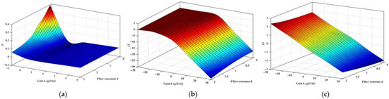
Figure 5. Solution of h(z) in Equation (32) with varying (K, d). (a) Solution of z₁; (b) Solution of z₂; (c) Solution of z₃.

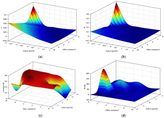
Figure 6. Solution of τ_k in Equation (26) with varying (K, d). (a) Calculation of A; (b) Calculation of B; (c) Calculation of arcsin(A/B); (d) Calculation of τ_k.

4.2. Control Design

In this section, the above analysis on the stabilization of the bio-process using washout-filter-aided control is conducted in theory. The flowchart describing a possible route to mitigate the Hopf bifurcation by means of a washout filter is provided in Figure 7, where open-loop oscillations could be eliminated once switching on the washout-filter-aided control at t = 2000 h (Figure 8). It is observed that the control ΔD = ΔF/V responds to the oscillations rapidly, and after the system is stabilized, the control action ΔD might approach zero, indicating the equilibrium state is preserved through washout-filter-aided control, though the open-loop equilibrium is unstable.

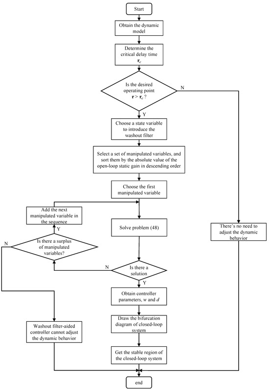
Figure 7. Flowchart of the proposed dynamic behavior adjustment method.

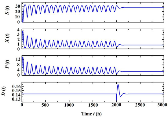
Figure 8. Simulation of the washout-filter-aided control on the self-oscillatory system, where K = 0.2 and d = 0.5.

It is worth mentioning that many research papers reported eliminating oscillations through control techniques [24], like PID or MPC, but only the proposed control preserves open-loop equilibrium, and once τ < τ_k is satisfied, a different control (K, d) would lead to the same static residual. As shown in Figure 8, the time-average ethanol concentration 3.37 g/L in the open-loop system is higher than the stabilized equilibrium concentration P* = 3.2 g/L, corresponding to the same dilution rate in the closed-loop system. This indicates that the oscillatory mode of operation can sometimes increase overall production, but the oscillatory system might shift to a washout condition and terminate the process, and oscillations need to be eliminated.

One problem with the proposed strategy is that the washout-filter-aided control is unable to achieve arbitrary set point tracking because it always converges to the equilibrium. Hence, Figure 9 is developed that presents the previous closed-loop system as an integral part, and an extra layer is added to realize set point tracking with PI control. Thus, the closed-loop system is altered to,

$$\left\{\begin{array}{l}{\displaystyle \frac{dS}{dt}}=D(S_{in}-S)-\sigma X=f_1\\ {\displaystyle \frac{dX}{dt}}=-DX+\mu X=f_2\\ {\displaystyle \frac{dP}{dt}}=-DP+\rho X=f_3\\ {\displaystyle \frac{dy}{dt}}=f_3-dy\\ {\displaystyle \frac{du}{dt}}={\displaystyle \frac{K}{T_i}}(P-P_{sp})\\ D(P,u)=K(P-P_{sp})+u\end{array}\right.$$

(32)

where k_p is the controller gain [L/g/h] and T_i > 0 is the controller integral time [h]; u represents the output signal for the integral part [1/h], and P_sp is the setpoint product (ethanol) concentration [g/L]. As shown in Figure 10, the closed-loop system (32), with extra k_p = 2 and T_i = 1, is stable without steady-state errors, irrespective of the chosen set point concentration.

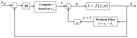
Figure 9. Configuration of the washout-filter-aided PI-control.

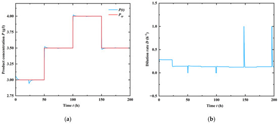
Figure 10. Responses of the closed-loop system to set point changes and the corresponding controller action for k_p = 2 [L/g/h] and T_i = 1 [h]. (a) Control performance of the given set-points; (b) Behavor of the manipulated variable, dilution rate.

Since the washout filter is triggered once perturbation information is detected, the effect of measurement noises should be properly addressed. In the case of ethanol on-line measurement, the measured signal can be corrupted by noise, especially if the ethanol concentration is determined in the gaseous phase. As shown in the previous section, high controller gain and low filter constant (approach zero) can stabilize the process with delay, but this would also lead to extensive control signal activity and the wear of the actuator in the presence of measurement noises. Inserting a 1st-order low-pass filter is also not advisable because the filter dynamics affect the stability and performance of the closed-loop system.

On the other hand, it is proven that a stable washout filter works well under measurement noises. To study the influence of noise on the closed-loop system, a white noise with a standard deviation σ = 0.08 [g/L] was added to the measured ethanol concentration, which is often observed when measuring the ethanol concentration on-line in the gaseous phase. For comparison purposes, the control and set-point trajectories are the same in Figure 10, and as shown in Figure 11, the effect of measurement noises can be greatly reduced under the proposed control, and the variations in the control signal can be reduced to an acceptable level.

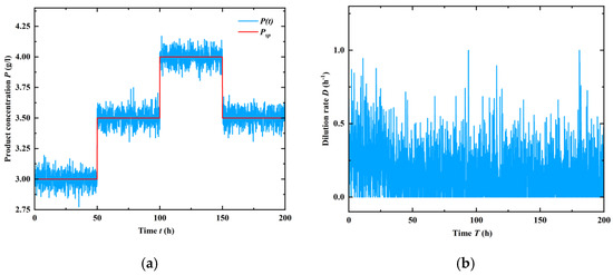
Figure 11. Tracking effect of adding measurement noises in control process. (a) Control performance of the given set-points; (b) Behavor of the manipulated variable, dilution rate.

5. Conclusions

This study tackles delay-induced self-oscillations in continuous ethanol fermentation, integrating Hopf bifurcation analysis and washout-filter-aided control to stabilize unstable dynamics. It is shown that delayed ethanol inhibition with intrinsic delay τ = 21.72 h introduces a critical delay threshold (τ_c = 20.97 h), beyond which Hopf bifurcations trigger oscillations. By deriving explicit criteria for τ_c, we linked instability to key process parameters, clarifying the role of microbial adaptation lags in destabilizing reactors. The proposed washout-filter-aided control strategy extends τ_c to 25.57 h (e.g., K = 2, d = 0.5), stably maintaining substrate 84.32 g/L, biomass 6.92 g/L, and ethanol 22.02 g/L concentrations without sacrificing productivity.

The proposed framework offers a mechanistic, scalable solution, leveraging intrinsic dynamics rather than additional hardware, making it suitable for industrial applications. Experimental validation underscores its robustness to parameter variations and noise, critical for real-world bioprocess control. Future work may explore multi-delay systems, adaptive control for time-varying delays, and integration with advanced techniques like model predictive control, further enhancing its utility in sustainable bio-manufacturing.

Future research will focus on methods/tools to be implemented to assess the stability status of general nonlinear, self-oscillatory systems, from the perspective of, say, robustness.

References

- Fiorentino, G.; Zucaro, A.; Ulgiati, S. Towards an energy efficient chemistry. Switching from fossil to bio-based products in a life cycle perspective. Energy 2019, 170, 720–729. [Google Scholar] [CrossRef]
- Li, S.; Hu, T.; Xu, Y.; Wang, J.; Chu, R.; Yin, Z.; Mo, F.; Zhu, L. A review on flocculation as an efficient method to harvest energy microalgae: Mechanisms, performances, influencing factors and perspectives. Renew. Sustain. Energy Rev. 2020, 131, 110005. [Google Scholar] [CrossRef]
- Chandel, A.K.; Garlapati, V.K.; Singh, A.K.; Antunes, F.A.F.; Da Silva, S.S. The path forward for lignocellulose biorefineries: Bottlenecks, solutions, and perspective on commercialization. Bioresour. Technol. 2018, 264, 370–381. [Google Scholar] [CrossRef]
- Ko, Y.-S.; Kim, J.W.; Lee, J.A.; Han, T.; Kim, G.B.; Park, J.E.; Lee, S.Y. Tools and strategies of systems metabolic engineering for the development of microbial cell factories for chemical production. Chem. Soc. Rev. 2020, 49, 4615–4636. [Google Scholar] [CrossRef]
- Zabed, H.M.; Akter, S.; Yun, J.; Zhang, G.; Awad, F.N.; Qi, X.; Sahu, J. Recent advances in biological pretreatment of microalgae and lignocellulosic biomass for biofuel production. Renew. Sustain. Energy Rev. 2019, 105, 105–128. [Google Scholar] [CrossRef]
- Boodhoo, K.; Flickinger, M.; Woodley, J.; Emanuelsson, E. Bioprocess intensification: A route to efficient and sustainable biocatalytic transformations for the future. Chem. Eng. Process.-Process Intensif. 2022, 172, 108793. [Google Scholar] [CrossRef]
- Martin-Lara, M.A.; Ronda, A. Implementation of modeling tools for teaching biorefinery (focused on bioethanol production) in biochemical engineering courses: Dynamic modeling of batch, semi-batch, and continuous well-stirred bioreactors. Energies 2020, 13, 5772. [Google Scholar] [CrossRef]
- Wang, J.; Chae, M.; Beyene, D.; Sauvageau, D.; Bressler, D.C. Co-production of ethanol and cellulose nanocrystals through self-cycling fermentation of wood pulp hydrolysate. Bioresour. Technol. 2021, 330, 124969. [Google Scholar] [CrossRef]
- Maxon, W.D. Continuous fermentation: A discussion of its principles and applications. Appl. Microbiol. 1955, 3, 110–122. [Google Scholar] [CrossRef]
- Lian, H.; Feng, E.; Li, X.; Ye, J.; Xiu, Z. Oscillatory behavior in microbial continuous culture with discrete time delay. Nonlinear Anal. Real World Appl. 2009, 10, 2749–2757. [Google Scholar] [CrossRef]
- Wang, L.; Zhao, X.-Q.; Xue, C.; Bai, F.-W. Impact of osmotic stress and ethanol inhibition in yeast cells on process oscillation associated with continuous very-high-gravity ethanol fermentation. Biotechnol. Biofuels 2013, 6, 133. [Google Scholar] [CrossRef]
- Tu, B.P.; Kudlicki, A.; Rowicka, M.; McKnight, S.L. Logic of the yeast metabolic cycle: Temporal compartmentalization of cellular processes. Science 2005, 310, 1152–1158. [Google Scholar] [CrossRef]
- Ferrell, J.E.; Tsai, T.Y.C.; Yang, Q. Modeling the cell cycle: Why do certain circuits oscillate? Cell 2011, 144, 874–885. [Google Scholar] [CrossRef] [PubMed]
- Hobley, T.J.; Pamment, N.B. Differences in response of Zymomonas mobilis and Saccharomyces cerevisiae to change in extracellular ethanol concentration. Biotechnol. Bioeng. 1994, 43, 155–158. [Google Scholar] [CrossRef] [PubMed]
- Li, C.C. Mathematical models of ethanol inhibition effects during alcohol fermentation. Nonlinear Anal. Theory Methods Appl. 2009, 71, e1608–e1619. [Google Scholar] [CrossRef]
- Jobses, I.M.L.; Egberts, G.T.C.; Luyben, K.; Roles, J.A. Fermentation kinetics of Zymomonasmobilis at high ethanol concentrations: Oscillations in continuous cultures. Biotechnol. Bioeng. 1986, 28, 868–877. [Google Scholar] [CrossRef]
- Xiu, Z.L.; Zeng, A.P.; Deckwer, W.D. Multiplicity and stability analysis of microorganisms in continuous culture: Effects of metabolic overflow and growth inhibition. Biotechnol. Bioeng. 1998, 57, 251–261. [Google Scholar] [CrossRef]
- Ma, Y.-F.; Xiu, Z.-L.; Sun, L.-H.; Feng, E.-M. Hopf bifurcation and chaos analysis of a microbial continuous culture model with time delay. Int. J. Nonlinear Sci. Numer. Simul. 2006, 7, 305–308. [Google Scholar] [CrossRef]
- Toro, J.C.O.; Dobrosz-Gómez, I.; Gómez-García, M.Á.; Prat, J.; Massana, I. A structured study on the dynamic bifurcation behavior of a continuous ethanol fermentor. Chem. Eng. Sci. 2021, 243, 116777. [Google Scholar] [CrossRef]
- Bruce, L.J.; Axford, D.B.; Ciszek, B.; Daugulis, A.J. Extractive fermentation by Zymomonas mobilis and the control of oscillatory behavior. Biotechnol. Lett. 1991, 13, 291–296. [Google Scholar] [CrossRef]
- Bai, F.W.; Chen, L.J.; Anderson, W.A.; Moo-Young, M. Parameter oscillations in a very high gravity medium continuous ethanol fermentation and their attenuation on a multistage packed column bioreactor system. Biotechnol. Bioeng. 2004, 88, 558–566. [Google Scholar] [CrossRef]
- Fatima, S.; Govardhan, B.; Kalyani, S.; Sridhar, S. Extraction of volatile organic compounds from water and wastewater by vacuum-driven membrane process: A comprehensive review. Chem. Eng. J. 2022, 434, 134664. [Google Scholar] [CrossRef]
- Cheng, Z. Anti-control of Hopf bifurcation for Chen’s system through washout filters. Neurocomputing 2010, 73, 3139–3146. [Google Scholar] [CrossRef]
- Skupin, P.; Metzger, M. PI control for a continuous fermentation process with a delayed product inhibition. J. Process Control 2018, 72, 30–38. [Google Scholar] [CrossRef]
- Hajaya, M.G.; Shaqarin, T. Multivariable advanced nonlinear controller for bioethanol production in a non-isothermal fermentation bioreactor. Bioresour. Technol. 2022, 348, 126810. [Google Scholar] [CrossRef]
- Chai, X.; Zong, K.; Zhai, C. Analyze and control on the membrane ethanol fermentation process with periodic exogenous signals. Chem. Eng. Process.-Process Intensif. 2022, 181, 109174. [Google Scholar] [CrossRef]
- Rapaport, A.; Dochain, D. Interval observers for biochemical processes with uncertain kinetics and inputs. Math. Biosci. 2005, 193, 235–253. [Google Scholar] [CrossRef]
- Petre, E.; Selisteanu, D.; Roman, M. Advanced nonlinear control strategies for a fermentation bioreactor used for ethanol production. Bioresour. Technol. 2021, 328, 124836. [Google Scholar] [CrossRef] [PubMed]
- Skupin, P.; Metzger, M. Stability analysis of the continuous ethanol fermentation process with a delayed product inhibition. Appl. Math. Model. 2017, 49, 48–58. [Google Scholar] [CrossRef]
- Song, Y.; Wei, J. Bifurcation analysis for Chen’s system with delayed feedbackand its application to control of chaos. Chaos Solitons Fractals 2004, 22, 75–91. [Google Scholar] [CrossRef]
- Zhang, N.; Seider, W.D.; Chen, B. Bifurcation control of high-dimensional nonlinear chemical processes using an extended washout-filter algorithm. Comput. Chem. Eng. 2016, 84, 458–481. [Google Scholar] [CrossRef]
- Villafuerte-Segura, R.; Itzá-Ortiz, B.A.; López-Pérez, P.A.; Alvarado-Santos, E. Mathematical model with time-delay and delayed controller for a bioreactor. Math. Methods Appl. Sci. 2023, 46, 248–266. [Google Scholar] [CrossRef]
- Zhai, C.; Yang, C.; Na, J. Bifurcation Control on the Un-Linearizable Dynamic System via Washout Filters. Sensors 2022, 22, 9334. [Google Scholar] [CrossRef] [PubMed]
- Ciesielski, A.; Grzywacz, R. Dynamic bifurcations in continuous process of bioethanol production under aerobic conditions using Saccharomyces cerevisiae. Biochem. Eng. J. 2020, 161, 107609. [Google Scholar] [CrossRef]
- Ruan, S.; Wei, J. On the zeros of transcendental functions with applications to stability of delay differential equations with two delays. Dyn. Contin. Discret. Impuls. Syst. Ser. B 2003, 10, 863–874. [Google Scholar] [CrossRef]
- Wang, J.; Chae, M.; Sauvageau, D.; Bressler, D.C. Improving ethanol productivity through self-cycling fermentation of yeast: A proof of concept. Biotechnol. Biofuels 2017, 10, 193. [Google Scholar] [CrossRef] [PubMed]
- Perego, L., Jr.; Dias, J.C.D.S.; Koshimizu, L.H.; de Melo Cruz, M.R.; Borzani, W.; Vairo, M.L.R. Influence of temperature, dilution rate and sugar concentration on the establishment of steady-state in continuous ethanol fermentation of molasses. Biomass 1985, 6, 247–256. [Google Scholar] [CrossRef]
Disclaimer/Publisher’s Note: The statements, opinions and data contained in all publications are solely those of the individual author(s) and contributor(s) and not of MDPI and/or the editor(s). MDPI and/or the editor(s) disclaim responsibility for any injury to people or property resulting from any ideas, methods, instructions or products referred to in the content. |
© 2025 by the authors. Licensee MDPI, Basel, Switzerland. This article is an open access article distributed under the terms and conditions of the Creative Commons Attribution (CC BY) license (https://creativecommons.org/licenses/by/4.0/).