Abstract
The discrete element method (DEM) is widely used to simulate the mechanical behavior of granular materials. Particle motion is governed by Newton’s second law, and position updates rely on numerical integration, whose accuracy and efficiency directly influence both the simulation scale and result reliability. In this study, three integration schemes—Verlet, central difference, and fourth-order Runge–Kutta—were implemented within an existing DEM framework to simulate the packing behavior of particles with varying shapes. Corresponding physical packing experiments were conducted, and numerical results were compared with experimental observations to evaluate differences in packing height, morphology, and process. Results show that the fourth-order Runge–Kutta scheme achieves the highest accuracy, with a packing height error of only 5.72% for spherical particles, albeit at a computational cost roughly 2–3 times that of the central difference scheme, making it suitable for high-precision, complex contact scenarios. In contrast, Verlet and central difference schemes are highly sensitive to particle shape, leading to considerable variation in simulation errors. The central difference approach is recommended for vertical displacement predictions in simple contact conditions, while Verlet is better suited for scenarios involving large instantaneous contact forces.
1. Introduction
The Discrete Element Method (DEM) has become a powerful numerical tool for investigating granular materials due to its ability to capture nonlinear contact, separation, and collision behaviors. In DEM, particle motion is governed by Newton’s second law, and the choice of time integration scheme directly influences numerical stability, energy conservation, computational efficiency, and accuracy. Cundall [1,2,3,4,5] first introduced DEM with an explicit central difference scheme, pioneering its application in granular material modeling. Building on this, Potyondy [6] developed an improved explicit integration approach for rock-like granular materials, incorporating complex interparticle bonds to better capture rock behavior, providing valuable insights for rock engineering applications. De Klerk [7] proposed a variationally based integration scheme that enhances stability and reliability in large-scale particle packing simulations, though its performance under complex conditions requires further study. Poot [8] introduced a Bayesian framework to model discretization errors, offering a probabilistic perspective for evaluating and optimizing integration results. Zhou [9] presented a spatiotemporal variational integration method based on absolute nodal coordinates, delivering efficient and accurate simulations for flexible structures such as beams. Li [10,11] proposed an asynchronous long-step computation method for overlapping particles, employing the Velocity–Verlet algorithm to solve motion equations, which demonstrates advantages in handling frame structures, large deformations, and nonlinear behavior. Despite these advances, DEM simulations of particle packing still face challenges. Recent studies continue to highlight the critical impact of integration scheme selection on simulation outcomes [12], yet systematic comparisons of integration schemes in terms of accuracy, efficiency, and applicability remain limited; validation for complex particle shapes and mechanical behaviors is insufficient; and existing methods show constraints in accommodating particle diversity. In particular, the performance of high-order methods like RK4 in complex granular flow scenarios is not well explored [13]. Therefore, investigating the performance and applicability of DEM integration schemes in particle packing simulations remains a critical research direction.
Packing experiments [14,15,16], as a classical approach for investigating granular material properties, provide a reliable empirical basis for validating integration schemes in DEM. Such experiments enable direct observation of macroscopic characteristics, including the morphology of particle assemblies. Wu [17] conducted sand packing experiments combined with DEM simulations to examine the effects of particle size distribution, shape, and contact parameters on packing behavior, confirming the consistency between numerical and experimental results. Kumar [18] through drum and packing tests, investigated the influence of particle shape, surface roughness, rotation speed, density, and particle size on packing characteristics. These studies not only identify key factors governing particle packing but also demonstrate that experimental results can serve as a trustworthy benchmark for assessing the accuracy and applicability of DEM integration schemes.
Among the available explicit schemes, the Verlet family, central difference method, and Runge–Kutta (RK) schemes are widely used. Verlet-type methods [19,20,21] exhibit good energy behavior and are suitable for strong-contact systems. The central difference method [22,23,24] offers high computational efficiency and is the most commonly used explicit method in DEM. The fourth-order Runge–Kutta method [25,26,27] provides excellent accuracy and generality for nonlinear dynamical systems, but its application within DEM remains relatively limited, and its performance in particle-packing problems has yet to be evaluated comprehensively.
In addition to these explicit schemes, alternative families of integrators—including implicit methods and symplectic integrators—have been widely studied. Implicit integration schemes, such as the Newmark-β method and the HHT-α method [28], possess unconditional stability, but their application to DEM requires solving large-scale nonlinear algebraic equations at every time step, leading to extremely high computational cost. Moreover, the frequent contact switching and non-smooth force fields inherent in DEM significantly weaken the advantages of implicit schemes. Symplectic integrators can strictly preserve the geometric structure of Hamiltonian systems [29,30,31]; however, collisions, damping, and other dissipative mechanisms in DEM introduce substantial energy loss and irreversible processes, breaking the structural preservation property of symplectic schemes. As a result, symplectic integrators are not suitable for the non-conservative nature of DEM systems.
Therefore, considering efficiency, implementability, and practical applicability, this study selects three representative explicit integration methods—Verlet, central difference, and fourth-order Runge–Kutta—and systematically compares their performance in particle-packing simulations involving different particle shapes. Compared with previous studies, this work achieves innovation in the following three aspects: (1) The fourth-order Runge–Kutta method is systematically introduced into DEM particle-packing simulations and compared with classical explicit schemes, clarifying its advantages and applicability boundaries; (2) An integrated experimental–numerical evaluation framework is established, enabling systematic analysis of integrator performance in terms of packing height, morphology, and particle motion trajectories; (3) Practical recommendations are proposed for selecting integration schemes under varying particle shapes, contact complexity, and accuracy requirements, providing guidance for optimizing DEM simulation strategies.
2. Packing Test Design
2.1. Test Objects
The packing test, as a classic test method, provides a reliable real-world basis for verifying the discrete element integration methods. Through packing tests, macro features such as the morphology of the particle packing body and micro information such as particle–particle contact can be visually obtained. By comparing the results of discrete element simulations with test data, the rationality and accuracy of the integration method can be effectively verified. By simulating the packing process of particles under gravity and comparing parameters such as packing height [32], iteration steps, and packing completion time between simulation and test, the performance of the integration method in simulating particle packing behavior can be thoroughly assessed. In this test, the specimens are made of rubberwood with moderate hardness, and its density is 650 kg/m3. Table 1 lists the different shapes and dimensions of the specimens used in the test. Three groups of packing tests were conducted, namely sphere–sphere, ellipsoid–ellipsoid, and cube–cube.

Table 1.
Specimen Styles and Dimensions.
2.2. Test Equipment and Materials
The test consists mainly of an observation device and a test container. The observation device comprises a high-speed camera (Phantom VEO-E 310L, Vision Research, Inc., Wayne, NJ, USA), a stand, and an LED light. The test container, shown in Figure 1, is made from acrylic sheets with high transparency to ensure good visibility during the test. The dimensions of the test container are 30 cm × 30 cm × 30 cm, and the top cover measures 35 cm × 35 cm × 2 cm. To ensure consistency and reproducibility of the packing process, a 6 cm × 6 cm hole is reserved at the center of the top cover as the entry point for objects during the packing test. Before the test begins, the frame rate of the high-speed camera is set to 200 frames per second, and the LED light is turned on to provide stable lighting. The camera is used to record the entire process of the specimen falling and packing.
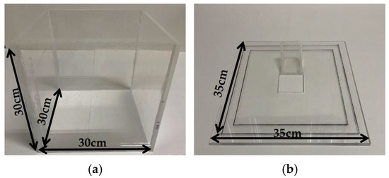
Figure 1.
Test container and top cover: (a) Test container; (b) Test cover.
In the packing test, a total of 100 specimens were used. Each specimen was released from a central opening in the top cover without initial velocity, with subsequent specimens introduced at 1 s intervals until all 100 units were deposited. For spherical and cubic specimens, which included two different sizes, an alternating sequence from smaller to larger particles was adopted during release. This alternating release strategy from smaller to larger particles helps simulate a more natural packing process for particle mixtures, preventing potential severe segregation that could result from a strict size-ordered release, thereby yielding a more representative random packing structure. Furthermore, this fixed release sequence enhances the reproducibility of the experimental process, providing stable and consistent initial conditions for precise comparisons across different test repetitions and with numerical simulation
After all specimens were deposited and the system reached a fully static state, the final packing height of each test group was recorded. Representative images of the packing process were extracted from high-speed camera footage to facilitate comparison with the numerical simulation results in terms of packing height and morphology. Each type of particle packing test was conducted five times, and the average packing height was taken as the final value for comparison with the numerical simulation results.
To account for potential measurement uncertainties, an assessment of the error in the final packing height readings was conducted. The primary sources of uncertainty were twofold: (1) human reading error, as the upper surface of the packing was not perfectly horizontal, introducing an estimated error of approximately ±0.2 cm when reading the scale by visual inspection; and (2) systematic error, including minor imperfections in the container’s base flatness and the influence of lens distortion from the high-speed camera. To minimize random errors, each packing test was repeated five times. The reported final packing height is the average value, with the standard deviation across all trials being less than 0.3 cm, indicating good reproducibility of the experimental results. The comparative analysis with numerical simulation results confirms that these measurement uncertainties are within an acceptable range and do not affect the subsequent qualitative and quantitative comparisons.
3. Contact Determination and Contact Force Model
3.1. Phase I Contact Determination
The contact detection algorithm between arbitrary geometries in the discrete element method can obtain contact characteristics such as the direction of the contact normal and the contact depth. These characteristics are used to calculate the contact force. The contact detection method is carried out in two steps: in the first stage, the bounding box method is used to traverse all elements in the system to obtain and record potential contact elements.
Phase I contact determination employs the bounding volume method [33,34], with the core objective of rapidly eliminating a large number of element pairs that cannot possibly be in contact, thereby significantly enhancing overall computational efficiency. In this method, an axis-aligned bounding box (AABB) is constructed for each discrete element.
The specific determination process is as follows: The bounding box of the current element is projected onto the three coordinate axes and compared with the projections of the bounding boxes of all other elements in the system. If the projected intervals of two bounding boxes overlap on all three coordinate axes, the corresponding element pair is considered potentially in contact. If the projections do not overlap on any one of the coordinate axes, the elements are determined to be non-contacting and are immediately excluded.
This method constitutes a conservative screening step. Although it may erroneously identify some non-contacting elements whose bounding boxes intersect as “candidate contacts,” it guarantees that no actually contacting elements are missed. Consequently, it provides a substantially reduced list of candidate element pairs for the subsequent phase of precise contact determination.
3.2. Phase II Contact Determination
In Phase II, precise contact determination is performed on the candidate contact pairs using the fast common plane (FCP) [35] method. The traditional common plane method requires iteratively rotating an initial plane to find the optimal plane separating two elements, which incurs high computational cost. The fast common plane method introduces a key improvement: it first constructs a candidate space containing all possible common planes based on the two closest vertices between the elements.
Subsequently, the method directly enumerates four possible geometric configurations for the common plane: the perpendicular bisector plane, a plane parallel to a face of one element, and a plane parallel to an edge from each element, among others. By calculating the gap values between the two elements under these candidate common planes and selecting the plane that yields the maximum gap as the final common plane, it avoids the time-consuming iterative “trial-and-error” process.
Once the common plane is determined, the contact state is evaluated by computing the gap values of the two elements relative to this plane: a negative gap indicates penetration (actual contact), while a gap smaller than a positive threshold suggests proximity contact. Concurrently, based on whether each element contacts the common plane at a point, along an edge, or on a face, the final contact type between them—such as point–point, point–edge, or edge–face contact—is determined. This information is then used to calculate the precise contact point and contact normal direction.
3.3. Element Contact Force Calculation
The contact force calculation is based on an explicit time integration scheme and utilizes the contact information provided by Phase II determination, which includes the contact depth , the normal direction , and the contact point . The normal contact force is modeled using a linear elastic formulation.
where is the normal contact stiffness of the elements, represents the contact depth between the elements and the negative sign indicates that the force acts in the direction opposite to the penetration.
The tangential contact force is calculated using an incremental algorithm, with consideration of friction effects. First, the tangential force increment is computed based on the relative motion at the contact point:
where is the tangential stiffness, and is the tangential relative velocity of element B with respect to element A at the contact point. This velocity is obtained by first combining the translational velocities and angular velocities of both elements’ centroids, and then removing the normal component. The tangential force at the current time step is calculated by adding this increment to the force from the previous time step, subject to the Coulomb friction limit:
where is the static friction coefficient, and is the unit vector in the tangential direction.
To simulate energy dissipation and enhance numerical stability, velocity-dependent damping forces are also introduced in the model. The contact damping force and damping moment are calculated as follows:
where and are the damping coefficients, while and represent the relative velocity and angular velocity at the contact point, respectively. The total force and moment on an element from a single contact pair are then obtained as:
where is the coordinates of the element’s centroid. If an element is simultaneously in contact with multiple other elements or boundaries, the forces and moments from all contact pairs are vectorially summed to obtain the net force and net moment acting on the element:
The net force and net moment are then substituted into the Newton–Euler equations of motion to update the acceleration, velocity, and position of the element for the current time step, thereby driving the dynamic evolution of the entire discrete system.
4. Comparison and Analysis of Simulation and Test Results
4.1. Code Implementation of Numerical Simulation
This study was conducted using the Visual Studio development platform with C++, leveraging the Standard Template Library (STL) and the OpenGL graphics library [36,37,38]. A comprehensive code framework has been developed capable of handling contact interactions among multiple element types and simulating the packing behavior of particles with various shapes. The code is well established and has demonstrated satisfactory performance in numerical simulations. To facilitate understanding of how the three integration schemes are implemented in this framework, pseudocode for the Verlet algorithm, the central difference method, and the fourth-order Runge–Kutta method is presented. The pseudocode preserves the core computational logic while omitting extensive programming details, providing a clear illustration of the steps involved in updating element positions and velocities.
Specifically, the Verlet algorithm updates particle positions directly based on their current and previous positions, without explicitly relying on velocity variables. Figure 2 presents the pseudocode and corresponding solution diagram for the Verlet algorithm are provided.
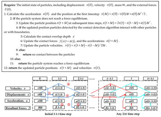
Figure 2.
Pseudocode and solution diagram of the Verlet integration algorithm.
The central difference method updates particle positions and velocities iteratively by alternately advancing half-step velocities and current positions, making it particularly suitable for the rapid simulation of large-scale particle systems. Figure 3 presents the pseudocode and corresponding solution diagram for the central difference method.
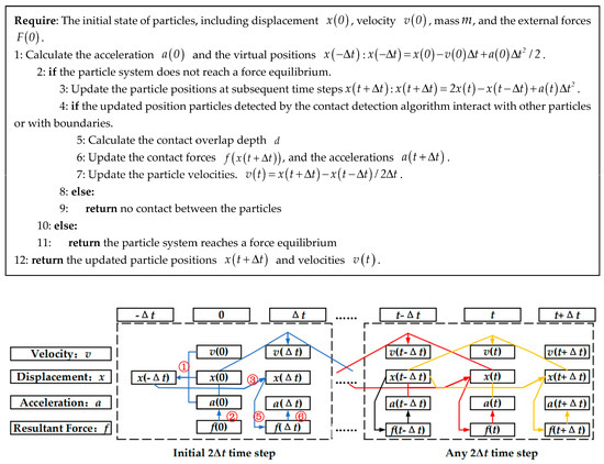
Figure 3.
Pseudocode and solution procedure of the central difference method.
The fourth-order Runge–Kutta method updates particle positions and velocities with higher accuracy by computing a weighted average of several intermediate slopes within each time step. Although this approach requires more computational effort, it provides superior generality and precision when dealing with complex contact interactions and nonlinear dynamics. Figure 4 presents the pseudocode and solution flowchart of the fourth-order Runge–Kutta method.
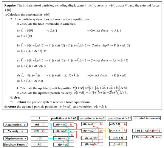
Figure 4.
Pseudocode and solution process of the fourth-order Runge–Kutta method.
After completing the implementation of the three integration schemes, each was embedded as an independent submodule into the existing particle packing simulation framework. This integration enabled flexible selection among multiple integration strategies, thereby enhancing the completeness and applicability of the simulation system. The extended code not only facilitates comparative analysis of different integration schemes but also provides a more versatile numerical tool for large-scale packing problems. Figure 5 presents the development flowchart of the packing simulation code for particles of various shapes, offering an intuitive illustration of the overall code development and integration process.
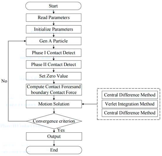
Figure 5.
Development Flowchart of the Packing Simulation Code for Particles with Different Shapes.
4.2. Numerical Simulation Parameter Setup
Before initiating the discrete element simulation, relevant computational parameters must be input. First, simulation parameters including particle type, material properties, and boundary dimensions are entered, followed by particle initialization. Subsequently, appropriate functions are used to generate the initial positions and shapes of the particles, thereby completing the initial packing configuration. Next, first-order and second-order contact detections are conducted sequentially. Based on these detections, inter-particle and particle–boundary contact forces are computed using the built-in contact force models. The motion and position updates of the particles are then performed by invoking different integration methods, and the convergence criteria are evaluated to determine whether to proceed with further iterations. Finally, once the termination conditions are met, simulation results are output, completing the entire discrete element simulation process.
The input parameters include particle simulation parameters, material parameters, and container boundary dimensions, with the particle size and container boundary dimensions being consistent with the sizes of the particles and containers used in the actual experiment. The remaining parameters used in the numerical simulation are listed in Table 2.
Table 2.
Particle parameter table.
In discrete element simulations, the choice of time step directly governs numerical stability and accuracy. For explicit integration schemes like the ones employed in this study, the time step must be smaller than a critical value to prevent numerical instability. This critical time step is typically governed by the highest natural frequency of the system, which is related to the contact stiffness and the particle mass. A widely used criterion in DEM is the Rayleigh time step, estimated as:
where is the particle radius, is the density, is the shear modulus, is a constant (often taken as 0.8766 for 3D), and is a safety factor (typically < 1) [39]. Alternatively, a more practical and conservative estimate is based on the duration of a binary collision, given by:
where is the effective mass of two contacting particles, is the normal contact stiffness, is the characteristic impact velocity, and is a safety factor (usually ≤ 0.2) [40].
Based on the material properties and contact parameters listed in Table 2, and applying the aforementioned criteria with a safety factor, the theoretical critical time step for our system was estimated to be on the order of 10−6 s. This theoretical foundation provides a unified and rigorous starting point for time-step selection, which is applicable to all explicit integration schemes, including Verlet, central difference, and Runge–Kutta methods. The stability of these methods is fundamentally limited by the same high-frequency dynamics of the system they are simulating.
To quantitatively verify this selection and assess solution sensitivity, a convergence study was conducted for the ellipsoidal particle case using the central difference method. The total system energy and the final packing height were monitored across different time steps, as shown in Figure 6. The results demonstrate that for time steps of 5 × 10⁻⁷ s and 1 × 10⁻⁶ s, the system energy decays smoothly without anomalous increases, and the final packing height converges to a stable value. In contrast, with a time step of 5 × 10⁻⁶ s, the total energy exhibits high-frequency oscillations, signaling the onset of numerical instability, and the packing height begins to deviate. When the time step exceeds the maximum time step listed in Figure 6 and continues to increase, divergence occurs. Particles in the entire system keep vibrating, and the final state cannot stabilize. This confirms that 1 × 10⁻⁶ s is within the stable and convergent regime for all three integration schemes under the investigated conditions. Conversely, reducing the time step to 5 × 10⁻⁷ s or smaller does not produce noticeable gains in stability or accuracy but substantially increases computation time. For example, simulating the packing of 100 particles with a time step of 1 × 10⁻⁶ s requires approximately 2.1 h, whereas halving the step to 5 × 10⁻⁷ s increases runtime to about 3.8 h, markedly reducing efficiency. While smaller steps may enhance the resolution of individual collisions, their benefits to overall packing accuracy are limited, making them impractical for large-scale simulations. Accordingly, 1 × 10⁻⁶ s is identified as a safe and effective critical time step for the integration schemes examined in this study.
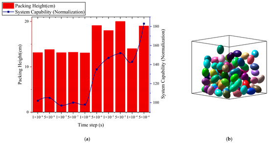
Figure 6.
Time Step Sensitivity Analysis: (a) Time Step Sensitivity Analysis (Spherical Particles) (b) Particles oscillate when the time step is too large.
4.3. Comparison and Analysis of Simulation Results with Experimental Data
4.3.1. Comparative Analysis of Stacking Morphology
Figure 7 illustrates the results of packing tests and numerical simulations for different particle shapes: (a) to (d) show spherical particle units, (e) to (h) show ellipsoidal particle units, and (i) to (l) show cubic particle units.
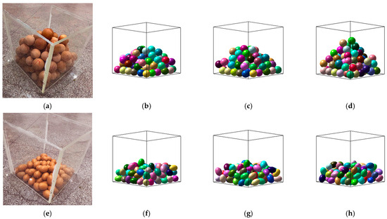
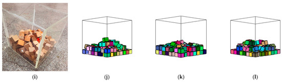
Figure 7.
Test and Simulation of Shape-Dependent Particle Packing: (a) Spherical Particle Packing Test; (b) Spherical Particle—Verlet Integration Method; (c) Spherical Particle—Central Difference Method; (d) Spherical Particle—Fourth-Order RK Method; (e) Ellipsoidal Particle Packing Test; (f) Ellipsoidal Particle—Verlet Integration Method; (g) Ellipsoidal Particle—Central Difference Method; (h) Ellipsoidal Particle—Fourth-Order RK Method; (i) Cubic Particle Packing Test; (j) Cubic Particles—Verlet Integration Method; (k) Cubic Particles—Central Difference Method; (l) Cubic Particles—Fourth-Order RK Method.
To better evaluate the state of particle accumulation, this study introduces the Root Mean Square Error (RMSE) as an indicator for assessing the packing process. When calculating the RMSE, the packing heights from the 50th particle onward are used. The rationale for this approach is as follows: in the initial stage of accumulation, most particles settle at the bottom of the container, resulting in minimal changes in packing height. It was observed that after approximately the 50th particle, the packing height inevitably undergoes noticeable changes, and clear discrepancies begin to emerge between experimental and numerical simulation data. Therefore, particles after the 50th are selected as representative. By doing so, the packing height data during the actual accumulation phase are fully incorporated into the calculation, allowing the RMSE to reflect, to a certain extent, the similarity in packing morphology.
Table 3 presents the test and simulated packing heights for different samples. As shown in Figure 7 and Figure 8, the packing of spherical particles is relatively concentrated, with localized tight contact. The simulation using the fourth-order Runge–Kutta (RK) method most closely resembles this, with both the test and simulated particles being more concentrated and forming a pyramid-like shape. The RMSE is 1.17, this finding provides further evidence supporting the conclusion that the fourth-order Runge–Kutta method yields a packing morphology in spherical particle simulations that most closely resembles that of the experimental tests. The relative error is 5.7%, demonstrating smaller errors compared to the other two integration methods. In contrast, the particles simulated using the other two integration methods are more evenly distributed, resulting in larger discrepancies compared to the test results. This highlights that the fourth-order RK method more accurately captures particle collisions and energy transfer, leading to localized clustering, while the other two methods exhibit greater numerical dissipation and are less sensitive to time step size, which causes the particles to be more uniformly distributed.
Table 3.
Test and Simulation Packing Heights of Different Specimens.
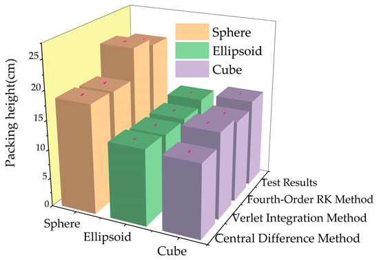
Figure 8.
Histogram of packing test and simulation results.
Ellipsoidal particles exhibit smaller packing voids and a more dispersed arrangement. In numerical simulations, all three integration methods successfully replicate the test packing patterns. However, simulations using the central difference method and Verlet integration show particles with steeper tilt angles, whereas the fourth-order Runge–Kutta (RK) method produces a flatter packing pattern, which is closer to the test results. The small RMSE value of the fourth-order Runge–Kutta method also numerically confirms this result. Regarding packing height, the central difference method yields a packing height of 13.07 cm, with the smallest error and RMSE. Combining the algorithm characteristics and multiple validations, our observations indicate that the central difference method is better at compensating for errors in the vertical direction for particles with smooth contact surfaces, making it more accurate in accumulating vertical displacement during complex collisions.
In the simulation of cubic particle packing with the three methods, the overall contour is consistent with the test results. However, the Verlet integration method more accurately reproduces the test features and contact states between particles in localized regions compared to the other two methods, with smaller errors in the packing height. This indicates that the Verlet integration method is well suited for simulating cubic particles. The reason lies in the fact that the contact between cubic particles is often instantaneous, with significant contact forces. Since the Verlet method updates the displacement directly without explicitly calculating velocity, it reduces numerical oscillations during intense contact, making the collision process smoother and more stable. On the other hand, the central difference method is more susceptible to numerical oscillations during high-speed collisions. Although the fourth-order Runge–Kutta method is theoretically more precise, its multiple evaluations of intermediate states may fail to effectively address the sudden changes in instantaneous forces during hard contact, leading to over-smoothing of local collision states and affecting the actual packing pattern of the particles.
4.3.2. Comparison Analysis of the Packing Process
To facilitate a comparison of the packing process, the position of a specific particle was tracked in real time during the test. By comparing the coordinate changes of the selected particle in both the test and simulation, the influence of different integration methods on the packing process was analyzed. In the test, a designated spherical particle was marked in red. When selecting the particle to be tracked, factors such as representativeness of its position, avoidance of boundary effects, and moderate variation of motion were considered to minimize potential errors.
Among all particles, the 30th particle was initially located in a typical central region, exhibiting representative motion and no abnormal behavior during its descent. Therefore, it was selected for tracking. Figure 9a–c show the packing configurations with 50, 75, and 100 particles, respectively. The corresponding positions of the designated particle in the simulations are shown in Figure 9d–f. These results indicate that the 30th particle is highly representative and suitable for tracking centroid coordinate changes. Figure 10a–c present the real-time coordinate variations of the tracked particle for spherical, ellipsoidal, and cubic shapes, respectively.
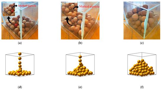
Figure 9.
Marked Spherical Particle Positions in Test and Simulation. (a) The packing consisted of 50 particles; (b) The packing consisted of 75 particles; (c) The packing consisted of 100 particles; (d) The simulation involved 50 particles; (e) The simulation involved 75 particles; (f) The simulation involved 100 particles.

Figure 10.
Centroid Coordinate Variation of Specified Shaped Particle. (a) Centroid Trajectory of the Marked Sphere; (b) Centroid Trajectory of the Marked Ellipsoid; (c) Centroid Trajectory of the Marked Cube.
It can be observed that the designated particle undergoes stages of free fall, collision translation, and rolling adjustment during the packing process, eventually stabilizing at the bottom layer of the packed structure. Its centroid coordinates decrease rapidly in the initial stage, undergo translation upon contacting the bottom particles, and gradually stabilize as the adjacent particles adjust.
The predictions of the centroid trajectory by the three integration methods generally align with the test particle trajectories, though some differences appear in the details. For all three shapes of particles, the centroid trajectory simulated by the fourth-order Runge–Kutta method is smooth, with the marked particle centroid trajectory and final position closely matching the test results, demonstrating excellent applicability and accuracy for all shapes.
The Verlet method’s simulation of the centroid trajectory is consistent with the test trend overall but shows a greater deviation from the test trajectory, particularly evident for spherical and cubic particles, indicating that while the Verlet method is applicable, it has some accuracy shortcomings.
The central difference method simulates the centroid coordinate change of spherical particles with minimal deviation, but shows significant differences when simulating ellipsoidal and cubic particles. This indicates that the central difference method performs well for packing simulations of simple shapes, but its applicability for complex shapes is relatively poor.
4.3.3. Comparison and Analysis of Computational Efficiency
To compare the computational efficiency of the three integration methods, the time required for simulating different shapes with each integration method was recorded at particle accumulations of the 0th, 5th, 10th, 15th, 20th, 25th, and 30th particles. By comparing the time spent for different integration methods to accumulate the same number of particles, the computational efficiency of each method can be analyzed. Figure 11 shows the computational time for different integration methods.
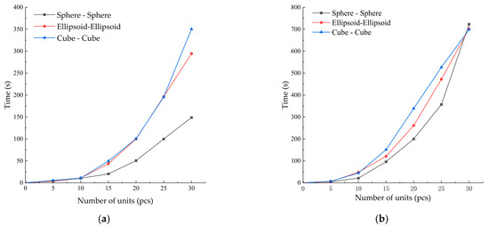
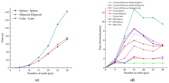
Figure 11.
Computational time comparison for different integration methods. (a) Central Difference Method; (b) Verlet Integration Method; (c) Fourth-Order Runge–Kutta Method; (d) Summary of the Three Methods. (Normalization).
From the simulation results, it can be seen that the central difference method required the least time during the accumulation of all types of particles, demonstrating the highest computational efficiency, making it suitable for large-scale and efficiency-prioritized simulation tasks. The Verlet method took slightly longer than the central difference method, offering a good balance between efficiency and stability. On the other hand, the fourth-order Runge–Kutta method, due to its complex computation process, required the most time under the same simulation conditions, resulting in the lowest computational efficiency.
In order to better compare the computational efficiency of these three integration methods in terms of quantity, we normalized the time. For the computation time of each method in a specific simulation scenario, we divided it by the time required by the central difference method for a sphere under the same conditions, setting this as the efficiency baseline. Theoretically, the central difference method requires the least number of floating-point operations per step. Due to its update sequence, the Verlet method requires slightly more computations; while the RK4 method is the most demanding, requiring four complete force evaluations per time step.
As shown in Figure 11d, Verlet Method shows a moderate increase in computational cost, with normalized times ranging from 1.27 to 2.0 for spheres, 1.43 to 4.68 for ellipsoids, and 1.81 to 4.30 for cubes. This aligns with its slightly more complex update logic. RK4 Method incurs the most substantial computational overhead, with normalized times ranging from 1.19 to 8.50 for spheres, 1.43 to 8.53 for ellipsoids, and 1.95 to 12.74 for cubes. The significant multipliers, especially at higher particle counts, directly correspond to its need for multiple intermediate force calculations per step.
This normalized comparison starkly illustrates the efficiency–accuracy trade-off. The Central Difference Method achieves the best computational performance, making it ideal for large-scale or efficiency-priority simulations. In contrast, the high accuracy of the RK4 method, as demonstrated in previous sections, comes at a cost of approximately 2.5 to over 12 times the computational effort of the baseline method, depending on particle count and shape complexity.
Moreover, the calculation error of RK4 could not reach the minimum in previous simulations of specific-shaped particles. Therefore, when choosing an integration method, the RK4 method, which has the highest accuracy, only achieves a relatively small error. However, this results in a multiple increase in computation time. Thus, one cannot rely solely on accuracy to roughly determine the choice of integration method. Selecting the integration method based on the specific applicable scenario can achieve both high efficiency and small error.
5. Conclusions and Future Work
This study systematically investigates the applicability and differences of various integration methods in simulating the packing behavior of particles with different shapes, by combining numerical simulation with test analysis. Based on the comparison between simulation results and test data, the following main conclusions are drawn:
- (1)
- The fourth-order Runge–Kutta method exhibits the highest accuracy, with a packing height error of only 5.72% for spheres. However, it is the least efficient, requiring approximately 2–3 times the computational time of the central difference method. It is recommended for high-precision simulations and complex contact scenarios.
- (2)
- The central difference method achieves the lowest error for ellipsoidal particles (6.20%) and the highest computational efficiency, making it suitable for large-scale systems or simulations where efficiency is prioritized. However, it shows larger errors in cube packing (16.37%), and is therefore recommended for vertical displacement predictions in simple contact scenarios.
- (3)
- The Verlet method’s accuracy is comparatively lower for spheres and ellipsoids, and it is thus recommended for scenarios involving large instantaneous contact forces.
Based on the findings of this study, several promising directions for future research are suggested. First, the integration schemes could be tested on more complex and irregular particle shapes (e.g., rods, plates, or custom-shaped aggregates) to further explore the relationship between shape complexity and integration accuracy. Second, investigating the performance and scalability of these methods in large-scale DEM systems with millions of particles would be valuable for industrial applications, potentially leveraging parallel computing and GPU acceleration. Furthermore, exploring adaptive time-stepping strategies or hybrid integration schemes that combine the strengths of different methods could be a fruitful path toward optimizing both efficiency and accuracy.
Author Contributions
Conceptualization, J.L.; methodology, J.L.; software, J.L. and Y.W.; formal analysis, P.Z.; data curation, P.Z.; writing—original draft preparation, P.Z.; writing—review and editing, J.L. and Y.W.; visualization, Y.W.; project administration, Y.W.; funding acquisition, Y.W. All authors have read and agreed to the published version of the manuscript.
Funding
This work was supported by the financial support from the Fundamental Research Funds for the Central Universities (Grant No. B250201198).
Data Availability Statement
The data presented in this study are available on request from the corresponding author.
Conflicts of Interest
The authors declare no conflicts of interest.
References
- Cundall, P.A.; Strack, O.D.L. Discussion: A discrete numerical model for granular assemblies. Géotechnique 1980, 30, 331–336. [Google Scholar] [CrossRef]
- Hadi, A.; Roeplal, R.; Pang, Y.; Schott, D.L. DEM Modelling of Segregation in Granular Materials: A Review. KONA Powder Part. J. 2023, 41, 78–107. [Google Scholar] [CrossRef]
- Liang, S.; Feng, Y.; Zhao, T.; Wang, Z. Review of numerical analysis methods for crushing behavior of particulate materials 1. Chin. J. Mech. 2024, 56, 1–22. [Google Scholar] [CrossRef]
- Ji, S.; Karlovšek, J. Calibration and uniqueness analysis of microparameters for DEM cohesive granular material. Int. J. Min. Sci. Technol. 2022, 32, 121–136. [Google Scholar] [CrossRef]
- Huang, L.; Deng, Q.; Wang, H. Instability behavior of loose granular material: A new perspective via DEM. Granul. Matter 2024, 26, 84. [Google Scholar] [CrossRef]
- Potyondy, D.O.; Cundall, P.A. A bonded-particle model for rock. Int. J. Rock Mech. Min. Sci. 2004, 41, 1329–1364. [Google Scholar] [CrossRef]
- Klerk, D.D.; Shire, T.; Gao, Z.; McBride, A.T.; Pearce, C.J.; Steinmann, P. A variational integrator for the Discrete Element Method. J. Comput. Phys. 2022, 462, 111253. [Google Scholar] [CrossRef]
- Poot, A.; Kerfriden, P.; Rocha, L.; Meer, F.V.D. A Bayesian approach to modeling finite element discretization error. Stat. Comput. 2024, 34, 167. [Google Scholar] [CrossRef]
- Zhou, P.; Ren, H.; Fan, W.; Zhang, Z. A spacetime variational integration approach to the full discretization of flexible beams based on absolute nodal coordinate formulation. Nonlinear Dyn. 2025, 113, 1175–1190. [Google Scholar] [CrossRef]
- Li, T.; Jin, X.; Wang, X.; Pan, J.; Yang, P. Parallel Computing Method of FEM-DEM with Multiple-time Step Based on Overlapping Boundary. Trans. Chin. Soc. Agric. Mach. 2023, 54, 419–426. [Google Scholar] [CrossRef]
- Li, T.; Wang, Q.; Jin, X. A Multi-time-step Discrete Element Method for Bar Structures. Chi. J. Comput. Phys. 2022, 39, 395–404. [Google Scholar] [CrossRef]
- Yu, M.; Kim, S.; Noh, G. Learned Gaussian quadrature for enriched solid finite elements. Comput. Methods Appl. Mech. Eng. 2023, 414, 116188. [Google Scholar] [CrossRef]
- Eshraghi1, H.; Amani, E.; Saffar-Avval, M. Coarse-graining algorithms for the Eulerian-Lagrangian simulation of particle-laden flows. J. Comput. Phys. 2023, 493, 112461. [Google Scholar] [CrossRef]
- Doan, T.; Indraratna, B.; Nguyen, T.T.; Rujikiatkamjorn, C. Interactive role of rolling friction and cohesion on the angle of repose through a microscale assessment. Int. J. Geomech. 2023, 23, 04022250. [Google Scholar] [CrossRef]
- Roessler, T.; Katterfeld, A. DEM parameter calibration of cohesive bulk materials using a simple angle of repose test. Particuology 2019, 45, 105–115. [Google Scholar] [CrossRef]
- Li, Y.; Xu, Y.; Thornton, C. A comparison of discrete element simulations and experiments for ‘sandpiles’ composed of spherical particles. Powder Technol. 2005, 160, 219–228. [Google Scholar] [CrossRef]
- Wu, W.; Guo, B.; Gao, Z.; Zheng, M.; Yang, H.; Li, D. Sand modeling and parameter calibration based on DEM. J. Chin. Agric. Mech. 2019, 40, 182–187. [Google Scholar] [CrossRef]
- Kumar, S.; Khatoon, S.; Yogi, J.; Verma, S.K.; Anand, A. Experimental investigation of segregation in a rotating drum with non-spherical particles. Powder Technol. 2022, 411, 117918. [Google Scholar] [CrossRef]
- Vyas, D.R.; Ottino, J.M.; Lueptow, R.M.; Umbanhowar, P.B. Improved Velocity-Verlet Algorithm for the Discrete Element Method. Comput. Phys. Commun. 2025, 310, 109524. [Google Scholar] [CrossRef]
- Lopez, S. An Explicit Time Integration Method Based on the Verlet Scheme with Improved Characteristics in Numerical Dispersion. J. Eng. Mech. 2024, 150, 04024031. [Google Scholar] [CrossRef]
- Ni, L.Y.; Hu, Z.H. On the relation between the velocity- and position-Verlet integrators. J. Chem. Phys. 2024, 161, 226101. [Google Scholar] [CrossRef]
- Wang, Z.; Liao, F.; Ye, Z. On Numerical Integration and Conservation of Cell-Centered Finite Difference Method. J. Sci. Comput. 2024, 100, 73. [Google Scholar] [CrossRef]
- Yang, H.F.; Chen, H.B.; Yue, X.Q.; Long, G.Q. High-order fractional central difference method for multi-dimensional integral fractional Laplacian and its applications. Commun. Nonlinear Sci. 2025, 145, 108711. [Google Scholar] [CrossRef]
- Guo, S.B.; Zhang, Z.Y. Numerical Methods Based on Characteristic Centered Finite Difference Procedure for a Class of Nonlinear Evolution Equations. Chin. J. Comput. Phys. 2024, 24, 637–646. [Google Scholar] [CrossRef]
- Daniel, D.; Lars, C.; Michael, S.L.; Gregor, J.G.; Manuel, T. Fourth-Order Paired-Explicit Runge-Kutta Methods. arXiv 2024, arXiv:2408.05470. [Google Scholar]
- Maneechay, P.; Khatbanjong, S.; Pochai, N.; Vongkok, A. Combination of the Fourth-Order Runge-Kutta and an Explicit Finite Difference Method for an Advection-Diffusion Equation. Eng. Lett. 2025, 33, 1251–1258. [Google Scholar]
- Krivovichev, G.V. Stability Optimization of Explicit Runge–Kutta Methods with Higher-Order Derivatives. Algorithms 2024, 17, 535. [Google Scholar] [CrossRef]
- Hilber, H.M.; Hughes, T.J.R.; Taylor, R.L. Improved numerical dissipation for time integration algorithms in structural dynamics. Earthq. Eng. Struct. Dyn. 1977, 5, 283–292. [Google Scholar] [CrossRef]
- Hairer, E.; Lubich, C.; Wanner, G. Geometric Numerical Integration: Structure Preserving Algorithms for Ordinary Differential Equations; Springer: Berlin/Heidelberg, Germany, 2004; pp. 817–821. [Google Scholar]
- D’Ambrosio, R.; Giordano, G.; Paternoster, B. Numerical conservation issues for stochastic Hamiltonian problems. In AIP Conference Proceedings; AIP Publishing LLC: Melville, NY, USA, 2022; Volume 2425, p. 090007. [Google Scholar] [CrossRef]
- Yoshida, H. Construction of higher order symplectic integrators. Phys. Lett. A 1990, 150, 262–268. [Google Scholar] [CrossRef]
- Liu, G.Y.; Xu, W.J.; Zhou, Q. DEM contact model for spherical and polyhedral particles based on energy conservation. Comput. Geotech. 2023, 153, 105072. [Google Scholar] [CrossRef]
- Indraratna, B.; Lackenby, J.; Christie, D. Effect of confining pressure on the degradation of ballast under cyclic loading. Geotechnique 2005, 55, 325–328. [Google Scholar] [CrossRef]
- Cundall, P.A. Formulation of a three-dimensional distinct element model—Part I. A scheme to detect and represent contacts in a system composed of many polyhedral blocks. Int. J. Rock Mech. Min. Sci. Geomech. Abstr. 1988, 25, 117–125. [Google Scholar] [CrossRef]
- Nezami, E.G.; Hashash, Y.M.A.; Zhao, D. A fast contact detection algorithm for 3-D discrete element method. Comput. Geotech. 2004, 31, 575–587. [Google Scholar] [CrossRef]
- Lei, X.; Ran, Y. A Fast Slicing Method for Colored Models Based on Colored Triangular Prism and OpenGL. Micromachines 2025, 16, 199. [Google Scholar] [CrossRef]
- Naseer, F.; Kazei, V.; Li, W. Understanding 3D seismic data visualization with C++, OpenGL and GLSL. Comput. Geosci. 2024, 191, 105681. [Google Scholar] [CrossRef]
- Xu, Z.; Zhang, C.; Zhou, S.; Yang, M.; Wu, H.; Li, J. GFNS: An OpenGL-based tool for shield tunneling simulation in 3D complex stratum. Comput. Geotech. 2024, 167, 106111. [Google Scholar] [CrossRef]
- O’Sullivan, C.; Bray, J.D. Selecting a suitable time step for discrete element simulations that use the central difference time integration scheme. Eng. Comput. 2004, 21, 278–303. [Google Scholar] [CrossRef]
- Kruggel-Emden, H.; Simsek, E.; Rickelt, S.; Wirtz, S.; Scherer, V. Review and extension of normal force models for the Discrete Element Method. Powder Technol. 2007, 171, 157–173. [Google Scholar] [CrossRef]


Disclaimer/Publisher’s Note: The statements, opinions and data contained in all publications are solely those of the individual author(s) and contributor(s) and not of MDPI and/or the editor(s). MDPI and/or the editor(s) disclaim responsibility for any injury to people or property resulting from any ideas, methods, instructions or products referred to in the content. |
© 2025 by the authors. Licensee MDPI, Basel, Switzerland. This article is an open access article distributed under the terms and conditions of the Creative Commons Attribution (CC BY) license (https://creativecommons.org/licenses/by/4.0/).