Cross-Line Transfer of Initial Juice Sugar Content Prediction Model for Sugarcane Milling

Abstract

Some sugar factories lack sufficient data collection in their milling production lines, making it challenging to construct data-driven models for predicting initial juice sugar content. This paper proposes an adversarial semi-supervised pre-training and fine-tuning modeling method. The model is first trained on data-rich source production lines (190,000 samples, 500 labels, 1 min sampling for process variables, 3 times/day for sugar content) and then fine-tuned using limited data from the target production line (10,000 samples, 100 labels), effectively utilizing both labeled and unlabeled data to enhance the model’s generalization ability. Ablation experiments were conducted using data from two sugarcane milling production lines. The experimental results validate the effectiveness of each component of the proposed method and its prediction accuracy, achieving a reduction in MSE by 0.067 (23.0%) and MAE by 0.066 (15.7%) compared to the standard pre-trained model. This strategy not only optimizes the prediction of initial juice sugar content for production lines with insufficient data collection but also has the potential to improve the efficiency and quality of sugarcane milling industrial production.

1. Introduction

Sugar content is the mass fraction of sugar dissolved in liquid. The initial juice sugar content is highest during sugarcane milling, significantly affecting the quality of the mixed juice and subsequent processes. It serves as a key indicator of sugarcane milling quality. A data-driven model to predict the initial juice sugar content enables more accurate production prediction, monitoring, and adjustment, leading to improved quality in the milling process.

Driven by the rapid advancement of artificial intelligence, data-driven modeling has garnered significant attention within the sugarcane milling industry. Numerous studies have demonstrated its potential for process optimization and quality prediction. For instance, Oktarini et al. [1] employed a Backpropagation Neural Network (BPNN) to predict sugarcane juice yield based on milling roll installation parameters. Meng et al. [2] utilized a Deep Knowledge-based Extreme Learning Machine (DK-ELM) to forecast the extraction rate and energy consumption in sugar factories. Li et al. [3] applied data-driven models to determine optimal operating conditions, while Qiu et al. [4] proposed a dual-layer multi-objective optimization method to enhance the sugarcane milling process. Furthermore, Yang et al. [5] introduced the TL-CNN-KELM framework for predicting both the milling extraction rate and the initial juice sugar content. More recently, Li et al. [6] combined deep learning with mechanistic models through a Physics-Informed Neural Network (PINN) to predict a series of key process indicators. These studies collectively provide a suite of effective data-driven modeling techniques that contribute to cost reduction, efficiency improvement, and quality enhancement in sugarcane production.

Despite these advancements, a significant challenge emerges when attempting to implement these data-driven models in practice, particularly concerning newly established or poorly digitized production lines. Technological progress often compels sugar factories to upgrade outdated equipment with advanced production lines to maintain competitiveness [7]. However, these new lines frequently suffer from a lack of sufficient historical data required for building robust data-driven models [8]. This issue of data scarcity is not unique to new lines; it also plagues production lines with a history of poor digital transformation or incomplete data records. Moreover, even when extensive data is available from one production line (the source line), the inherent differences in equipment specifications, operational parameters, and raw material characteristics between lines result in distinct data distributions. This phenomenon, known as domain shift, makes it difficult to directly apply a model trained on a source line to a different target line without a significant drop in performance. This highlights the urgent need for research focused on effective model transfer across different sugarcane milling production lines.

Transfer learning, particularly the pre-training and fine-tuning strategy, presents a promising solution to the aforementioned challenge. This strategy involves pre-training a model on a large-scale dataset from a source domain (e.g., a data-rich production line) to learn general feature representations. The pre-trained model is then fine-tuned using a limited amount of data from the target domain (e.g., a data-scarce production line), allowing it to adapt to the specific characteristics of the new environment [9]. This paradigm has been successfully applied in various fields where data collection is costly or limited, such as medicine and other industrial sectors [10,11,12,13], demonstrating its potential to enhance model performance and reduce reliance on large target-domain datasets.

Another critical aspect of the problem in sugarcane milling is the scarcity of labeled data. The initial juice sugar content is typically obtained through infrequent laboratory tests, resulting in a much lower sampling frequency compared to real-time monitoring parameters. This creates a scenario with a large volume of unlabeled data and only a small number of labeled samples. To leverage this abundant unlabeled data, semi-supervised learning (SSL) methods are highly relevant. Early work by Yarowsky [14] demonstrated the effectiveness of self-training for utilizing unlabeled data. In recent years, Generative Adversarial Networks (GANs) have introduced a powerful new perspective to SSL [15]. GANs can generate realistic synthetic samples and have been effectively adapted for semi-supervised scenarios, significantly improving model performance by learning the underlying data distribution from both labeled and unlabeled examples [16,17,18].

Given the complementary strengths of transfer learning and semi-supervised learning, their integration is a logical and promising approach to address the cross-line prediction problem for initial juice sugar content. This combination is expected to facilitate knowledge transfer from data-rich source lines while fully exploiting the unlabeled data available in the target line. Some preliminary progress has been made in integrating these two paradigms. For example, Abuduweili et al. [19] proposed an adaptive consistency regularization framework that leverages pre-trained models and unlabeled data. Sun and Qiao [20] developed a semi-supervised transfer learning strategy (KMCO) for fake review identification, although it targets classification problems rather than regression. However, despite these advances, there is a conspicuous lack of research on semi-supervised transfer learning strategies specifically designed for regression problems in industrial settings. More importantly, no existing method effectively addresses the data-driven modeling challenges for predicting initial juice sugar content across different sugarcane milling lines, which involves dealing with covariate shift and extreme label scarcity in both source and target domains.

In light of this research gap, this paper proposes a novel strategy that integrates adversarial semi-supervised learning with the pre-training and fine-tuning transfer learning framework. The specific contributions of this work are threefold:

1.

Pre-training and Fine-tuning Strategy: We employ a transfer learning strategy where a model is first pre-trained on a source production line with abundant data and subsequently fine-tuned using a small amount of data from the target production line. This approach mitigates the performance degradation caused by domain shift.

2.

Integration of Adversarial Semi-Supervised Learning: We incorporate adversarial semi-supervised learning during both the pre-training and fine-tuning stages. This allows the model to fully leverage the information contained within the vast amounts of unlabeled data present in both domains, thereby enhancing the model’s generalization capability.

3.

Experimental Validation: We conduct comprehensive experiments using real-world data from two sugarcane milling production lines. The results validate the predictive effectiveness of the proposed method. Furthermore, ablation studies are performed to confirm the individual contribution of each key component of our approach.

The remainder of this paper is organized as follows: Section 2 describes the data and elaborates on the proposed methodology. Section 3 presents the experimental results and discussions. Finally, Section 4 concludes the paper.

2. Data and Methods

2.1. Sugarcane Milling Data

The sugarcane milling process in a sugar factory typically includes operations such as unloading, pre-cutting, tearing, milling, and penetration. Data from two production lines, A and B, of a sugar factory in Guangxi, China, were selected for this study. Real-time monitoring data from these two lines were used as input to predict the initial juice sugar content. The real-time monitoring data collected covers nine variables, including instantaneous milling volume, percolating water flow volume, mixed juice flow volume, pre-cutter current, #1 crusher current, #1 squeezer current, #1 conveyor belt motor speed, #2 conveyor belt motor speed, and current stop time. The sampling frequency for each variable is 1 sample per minute. The electrical current data of the machinery directly reflects the power consumption of the equipment. The instantaneous milling volume and the conveyor belt motor speed reflect the input status of the sugarcane material. The pre-cutter and crusher currents show the degree of sugarcane crushed, and the squeezer current reflects the milling power. The flow volume of the mixed juice and the percolating water can be used to estimate the flow volume of the initial juice. The current downtime represents the time of machine stoppage within a minute. These factors have been proven to be correlated with the quality indicators of sugarcane milling, both in practice and through data-driven modeling. In addition, the shift report includes quality indicator data, such as extraction rate, initial juice sugar content, mixed juice sugar content, and bagasse moisture, with a sampling frequency of three samples per day. In this paper, the initial juice sugar content is selected as the target for prediction. The variable names, units, and sampling Interval for each variable are shown in Table 1.

Table 1. Variables Used in Sugarcane Milling Process Monitoring and Prediction.

Variable Name	Unit	Sampling Interval
Instantaneous Milling Volume	t/min	1 min
Percolating Water Flow Volume	m3/h	1 min
Mixed Juice Flow Volume	m3/h	1 min
Pre-cutter Current	A	1 min
#1 Crusher Current	A	1 min
#1 Squeezer Current	A	1 min
#1 Conveyor Belt Motor Speed	RPM	1 min
#2 Conveyor Belt Motor Speed	RPM	1 min
Current Stop Time	s	1 min
Initial Juice Sugar Content	%	3 times/day

2.2. Problem Definition

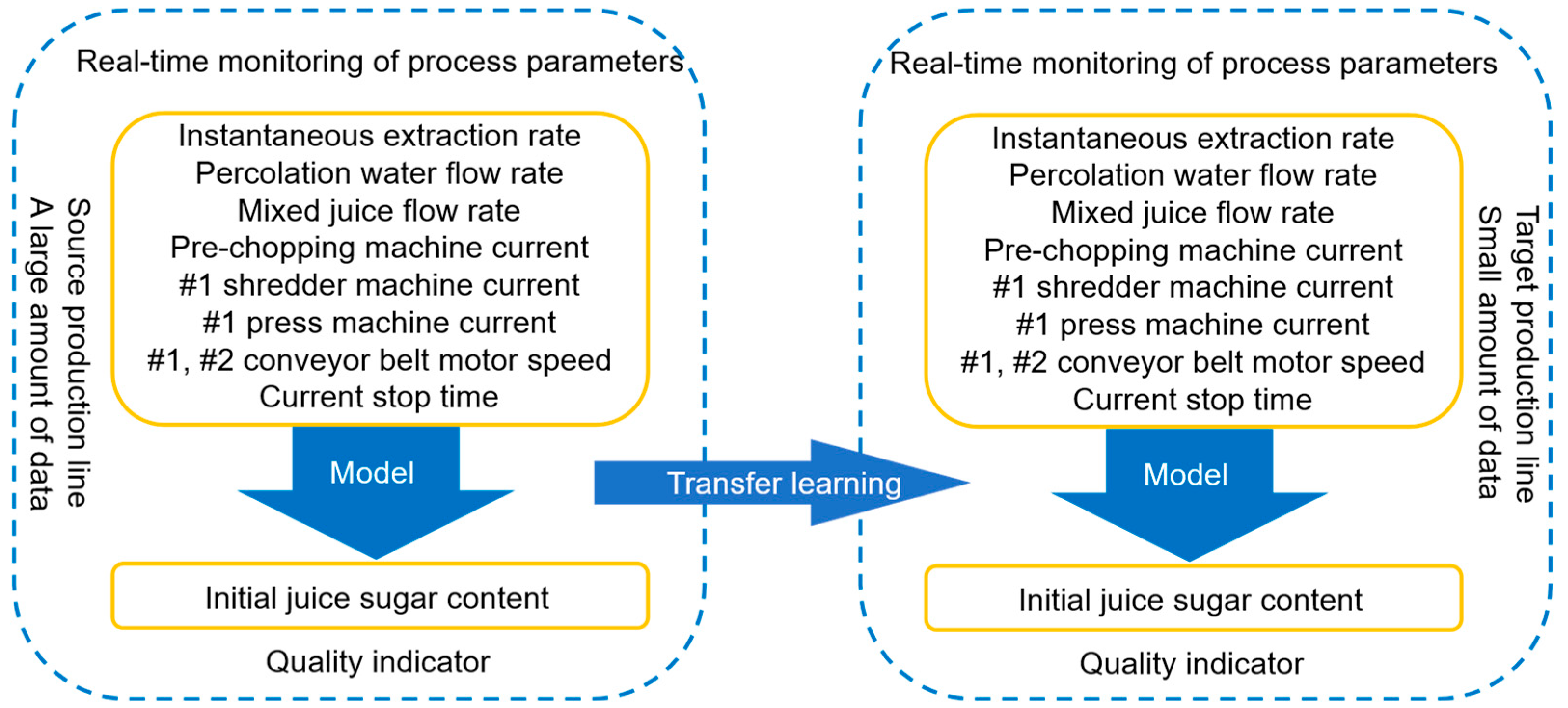
The sugarcane milling cross-line model transfer is a typical transfer learning task, which requires the data-driven model from the source production line to be transferred to the target production line, as shown in Figure 1.

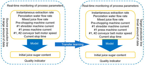
Figure 1. Schematic diagram of the cross-production line task for predicting initial juice sugar content.

Consequently, the data from the source production line can be utilized as the source domain data ${\mathsf{𝒟}}_{\mathrm{s}}=\{{𝒳}_{\mathrm{s}},{𝒴}_{\mathrm{s}}\}$, while the data from the target production line can be employed as the target domain data ${\mathsf{𝒟}}_{\mathrm{t}}=\{{𝒳}_{\mathrm{t}},{𝒴}_{\mathrm{t}}\}$. The sugarcane milling cross-line model transfer task is characterized as follows:

1.

The source production line data is abundant, while the target production line data is scarce, that is $N_{\mathrm{s}}$ ≫ $N_{\mathrm{t}}$, $M_{\mathrm{s}}$ ≫ $M_{\mathrm{t}}$.

2.

There is an abundance of unlabeled data, while labeled data is scarce, i.e., $N_{\mathrm{s}}$ ≫ $M_{\mathrm{s}}$, $N_{\mathrm{t}}$ ≫ $M_{\mathrm{t}}$.

3.

Domain Adaptation Problem: The feature space and target space are identical, i.e., ${𝒳}_{\mathrm{s}}={𝒳}_{\mathrm{t}}$ and ${𝒴}_{\mathrm{s}}={𝒴}_{\mathrm{t}}$. However, the joint probability distributions differ, as $P_{\mathrm{s}}(x,y)\ne P_{\mathrm{t}}(x,y)$.

4.

Covariate Shift, specifically manifested as $P_{\mathrm{s}}(x)\ne P_{\mathrm{t}}(x)$.

5.

The conditional probability distributions are similar, i.e., $P_{\mathrm{s}}(x|y)\approx P_{\mathrm{t}}(x|y)$.

Where $N_{\mathrm{s}}$ and $N_{\mathrm{t}}$ represent the quantity of samples in the source and target domains, respectively, while $M_{\mathrm{s}}$ and $M_{\mathrm{t}}$ represent the quantity of labels in the source and target domains, respectively, $(x,y)$ represents a sample. The task of sugarcane milling cross-line model transfer refers to the construction of a model using the aforementioned characteristic data, which aims to achieve optimal predictive performance in the target domain.

2.3. Pre-Training and Fine-Tuning

During the pre-training phase, the model is trained on a large-scale dataset, learning the general feature representations of the data. These features are capable of capturing the fundamental structures and common patterns within the data, laying the groundwork for knowledge sharing across various tasks.

Generally, the partial fine-tuning strategy within the pre-training and fine-tuning strategies is the most widely applied. The process is as follows:

There exists a source task and a target task, with the model parameters of the source task denoted as ${\theta }_{\mathrm{s}}$ and those of the target task denoted as ${\theta }_{\mathrm{t}}$. The loss function for the source task is expressed as $L_{\mathrm{s}}({\theta }_{\mathrm{s}};x_{\mathrm{s}},y_{\mathrm{s}})$, and the loss function for the target task is expressed as $L_{\mathrm{t}}({\theta }_{\mathrm{t}};x_{\mathrm{t}},y_{\mathrm{t}})$, where $x$ and $y$ represent the inputs and outputs, respectively.

During the pre-training phase, minimize the loss function of the source task:

$${\theta }_{\mathrm{s}}^{*}=\arg {\min }_{{\theta }_{\mathrm{s}}}{\displaystyle \frac{1}{N_{\mathrm{s}}}}{\displaystyle \sum _{i=1}^{N_{\mathrm{s}}}{L}_{\mathrm{s}}}({\theta }_{\mathrm{s}};x_{{\mathrm{s}}_i},y_{{\mathrm{s}}_i})$$

(1)

The fine-tuning phase involves precise optimization for a specific task based on the pre-trained model. During the fine-tuning phase, the objective is to find a new set of parameters ${\theta }_{\mathrm{t}}$ that minimizes the loss for the target task while leveraging the knowledge learned from the source task. This is typically achieved by freezing the initial layers of the pre-trained model and training only the final layer or layers.

The fine-tuned loss function can be expressed as:

$${\theta }_{\mathrm{t}}^{*}=\arg {\min }_{{\theta }_{\mathrm{t}}}{\displaystyle \frac{1}{N_{\mathrm{t}}}}{\displaystyle \sum _{i=1}^{N_{\mathrm{t}}}{L}_{\mathrm{t}}}({\theta }_{\mathrm{t}};x_{{\mathrm{t}}_i},y_{{\mathrm{t}}_i})$$

(2)

2.4. Adversarial-Based Semi-Supervised Learning

The core objective of semi-supervised learning is to fully utilize unlabeled data in the presence of only a small amount of labeled data, thereby enhancing the model’s performance under limited labeled data conditions. In the traditional GAN framework, the training of the generator and discriminator relies solely on labeled data. However, in adversarial-based semi-supervised learning, unlabeled data is also effectively incorporated into the training process.

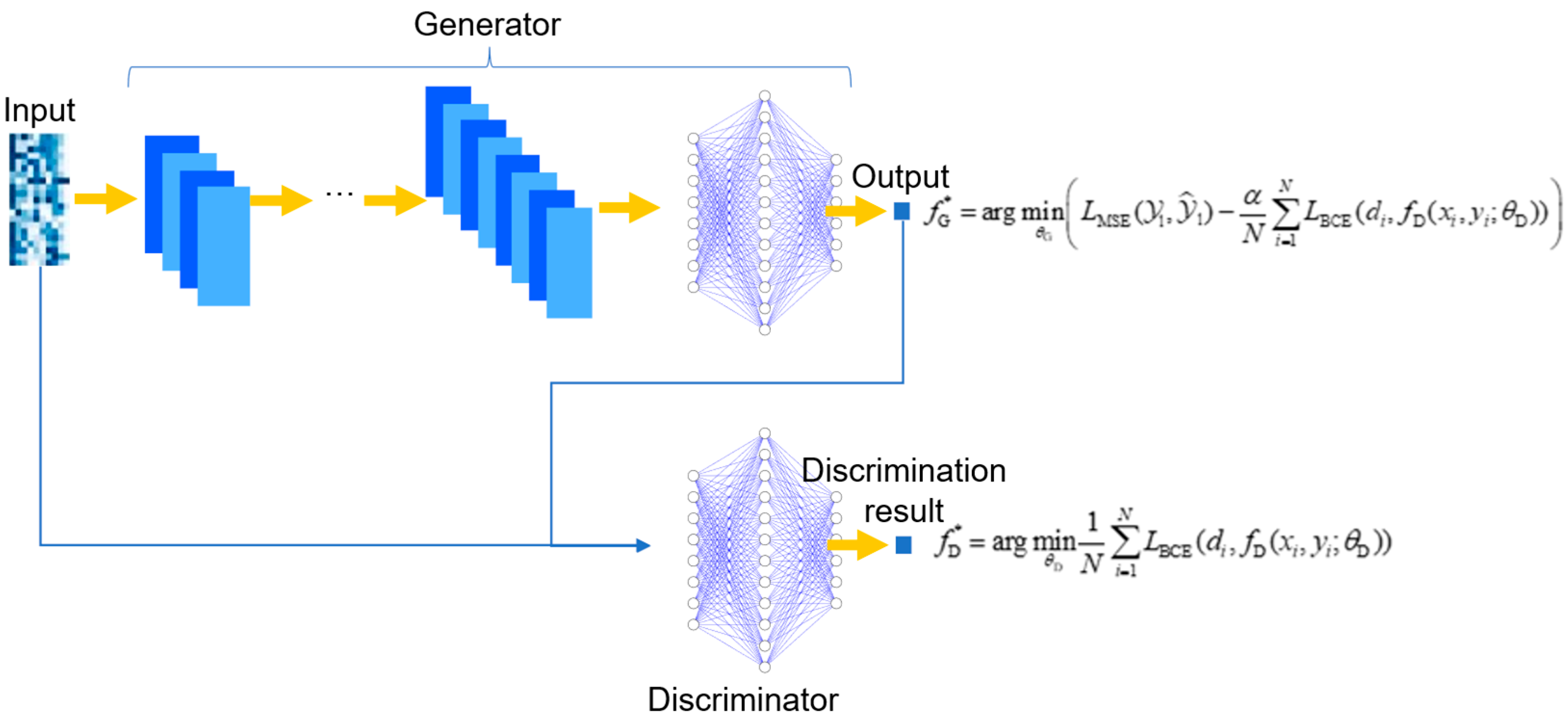
In this paper, the adversarial semi-supervised learning is illustrated in Figure 2 and is implemented through the following methods:

Figure 2. Schematic diagram of Semi-Supervised Learning based on an adversarial approach.

(1)

Input the labeled data ${𝒳}_{\mathrm{l}}$ and the unlabeled data ${𝒳}_{\mathrm{u}}$ into the generator to obtain the predictions ${\widehat{𝒴}}_{\mathrm{l}}$ for the labeled data and the pseudo-labels ${\widehat{𝒴}}_{\mathrm{u}}$ for the unlabeled data.

(2)

Input the labeled data ${𝒳}_{\mathrm{l}}$ and their ground-truth labels ${𝒴}_{\mathrm{l}}$, as well as the unlabeled data ${𝒳}_{\mathrm{u}}$ and their pseudo-labels ${\widehat{𝒴}}_{\mathrm{u}}$ (generated by the generator) into the discriminator. The discriminator determines whether the labels (${𝒴}_{\mathrm{l}}$ or ${\widehat{𝒴}}_{\mathrm{u}}$) paired with the input data (${𝒳}_{\mathrm{l}}$ or ${𝒳}_{\mathrm{u}}$) are real (ground-truth) or pseudo.

(3)

Optimize the discriminator using the following objective function to determine as accurately as possible whether the sample is a labeled sample:

$$f_{\mathrm{D}}^{*}=\arg \underset{{\theta }_{\mathrm{D}}}{\min }{\displaystyle \frac{1}{N}}{\displaystyle \sum _{i=1}^N{L}_{\mathrm{BCE}}}(d_i,f_{\mathrm{D}}(x_i,y_i;{\theta }_{\mathrm{D}}))$$

(3)

where ${\theta }_{\mathrm{D}}$ represents the parameters of the discriminator, $N$ represents the total number of samples, $d_i$ is a binary indicator variable: $d_i=1$ if the label for sample $i$ is a ground-truth measurement, and $d_i=0$ if it is a pseudo-label. $f_{\mathrm{D}}(x_i,y_i;{\theta }_{\mathrm{D}})$ is the discriminator’s estimated probability that the label $y_i$ for input $x_i$ is real. $L_{\mathrm{BCE}}(\cdot ,\cdot )$ represents the binary cross-entropy loss function, which is used to measure the difference between the discriminator’s judgment and the actual situation, specifically as follows:

$$L_{BCE}(d,D)=-[d\cdot \log (D)+(1-d)\cdot \log (1-D)]$$

(4)

(4)

Optimize the generator using the following objective function, enabling the generator to accurately predict labeled data while also deceiving the discriminator as much as possible to generate more “realistic” pseudo-labels for unlabeled data, thereby enhancing the generalization ability of the generator:

$$f_{\mathrm{G}}^{*}=\arg \underset{{\theta }_{\mathrm{G}}}{\min }\left(L_{\mathrm{MSE}}({𝒴}_{\mathrm{l}},{\widehat{𝒴}}_{\mathrm{l}})-{\displaystyle \frac{\alpha }{N}}{\displaystyle \sum _{i=1}^N{L}_{\mathrm{BCE}}}(d_i,f_{\mathrm{D}}(x_i,y_i;{\theta }_{\mathrm{D}}))\right)$$

(5)

where ${\theta }_{\mathrm{G}}$ represents the parameters of the generator, $\alpha$ is the adversarial weight coefficient, a key hyperparameter that balances the contribution of the supervised loss and the adversarial loss, thus governing the update focus of the generator. ${\widehat{𝒴}}_{\mathrm{l}}$ is the predicted value of the labeled data, which is a function of the generator parameters ${\theta }_{\mathrm{G}}$, that is, ${\widehat{𝒴}}_{\mathrm{l}}=f_{\mathrm{G}}({𝒳}_{\mathrm{l}};{\theta }_{\mathrm{G}})$, $L_{\mathrm{MSE}}({𝒴}_{\mathrm{l}},{\widehat{𝒴}}_{\mathrm{l}})$ represents the prediction loss of the labeled data, which generally refers to the mean squared error loss in regression problems, that is:

$$L_{\mathrm{MSE}}({𝒴}_{\mathrm{l}},{\widehat{𝒴}}_{\mathrm{l}})={\displaystyle \frac{1}{N}}{\displaystyle \sum _{i=1}^N{(y_i-{\widehat{y}}_i)}^2}$$

(6)

(5)

By alternately optimizing steps 3 and 4, the generator and discriminator are balanced, ultimately resulting in a well-trained generator model that can be used for prediction tasks. The specific implementation process for adversarial semi-supervised learning is detailed in Algorithm 1.

Algorithm 1 Adversarial-based semi-supervised learning

Input: $X_{\mathrm{l}}$—Labeled feature set $Y_{\mathrm{l}}$—Labeled label set $X_{\mathrm{u}}$—Unlabeled feature set $\alpha$—Generator loss weight $nu{m}_{\mathrm{iterations}}$—Number of iterations $D_{\mathrm{steps}}$—Discriminator update steps per round $G_{\mathrm{steps}}$—Generator update steps per round   Output: ${\theta }_{\mathrm{G}}^{\mathrm{final}}$—Final generator parameters   Begin Initialize ${\theta }_{\mathrm{G}}$$, {\theta }_{\mathrm{D}}$ For iteration = 1 to $nu{m}_{\mathrm{iterations}}$:  Generator prediction: Generate predictions for labeled and unlabeled data  $\mathrm{For} \mathrm{step} = 1 \mathrm{to} D_{\mathrm{steps}}$:   Compute and accumulate discriminator loss on labeled and unlabeled data   $\mathrm{Update} {\theta }_{\mathrm{D}}$  For step = 1 to $G_{\mathrm{steps}}$:   Compute and accumulate generator loss on labeled data   Compute and accumulate generator adversarial loss on unlabeled data   $\mathrm{Update} {\theta }_{\mathrm{G}}$ ${\theta }_{\mathrm{G}}^{\mathrm{final}}$ $= {\theta }_{\mathrm{G}}$ End

2.5. Adversarial Semi-Supervised Pre-Training Fine-Tuning Strategy

The adversarial semi-supervised pre-training and fine-tuning strategy used in this paper applies adversarial-based semi-supervised learning in both the pre-training and fine-tuning stages of transfer learning to better address the issue of sparse label data in both the source and target domains. Specifically:

During the pre-training phase, a large amount of unlabeled data and a small amount of labeled data from the source domain are modeled using an adversarial semi-supervised learning method. Both the feature extractor $f_{\mathrm{FE}}(\cdot )$ and the predictor $f_{\mathrm{RP}}(\cdot )$ of the model are trained simultaneously as the generator in the adversarial framework. Additionally, a discriminator $f_D(\cdot )$ is constructed to distinguish between real labels and pseudo labels, and the predicted values of the source domain data are

$${\widehat{𝒴}}_{\mathrm{s}}=f_{\mathrm{RP}}(f_{\mathrm{FE}}({𝒳}_{\mathrm{s}},{\theta }_{\mathrm{FE}}),{\theta }_{\mathrm{RP}})$$

(7)

where ${\theta }_{\mathrm{FE}}$ and ${\theta }_{\mathrm{RP}}$ represent the parameters of the feature extractor and the predictor, respectively, optimized through the following discriminator and generator objective functions:

Discriminator objective

$$f_{\mathrm{sD}}^{*}=\arg \underset{{\theta }_{\mathrm{D}}}{\min }{\displaystyle \frac{1}{N_{\mathrm{s}}}}{\displaystyle \sum _{i=1}^{N_{\mathrm{s}}}{L}_{\mathrm{BCE}}}(d_{\mathrm{s}i},f_{\mathrm{sD}}(x_{\mathrm{s}i},y_{\mathrm{s}i};{\theta }_{\mathrm{D}}))$$

(8)

Generator objective:

$$f_{\mathrm{sG}}^{*}=\arg \underset{{\theta }_{\mathrm{FE}},{\theta }_{\mathrm{RP}}}{\min }\left(L_{\mathrm{MSE}}({𝒴}_{\mathrm{sl}},{\widehat{𝒴}}_{\mathrm{sl}})-{\displaystyle \frac{\alpha }{N_{\mathrm{s}}}}{\displaystyle \sum _{i=1}^{N_{\mathrm{s}}}{L}_{\mathrm{BCE}}}(d_{\mathrm{s}i},f_{\mathrm{sD}}(x_{\mathrm{s}i},y_{\mathrm{s}i};{\theta }_{\mathrm{D}}))\right)$$

(9)

A pre-trained model with good generalization performance applicable to source domain data is ultimately obtained.

In the fine-tuning phase, modeling is conducted using adversarial-based semi-supervised learning with fewer unlabeled and labeled data from the target domain relative to the source domain. Only the predictor part of the model, denoted as $f_{\mathrm{RP}}(\cdot )$, is trained, and the predicted values for the target domain are

$${\widehat{𝒴}}_{\mathrm{t}}=f_{\mathrm{RP}}(f_{\mathrm{FE}}({𝒳}_{\mathrm{t}},{\theta }_{\mathrm{FE}}),{{\theta }_{\mathrm{RP}}}^{\prime })$$

(10)

The parameter ${{\theta }_{\mathrm{RP}}}^{\prime }$ of the predictor, after fine-tuning with target domain data, is optimized through the following discriminator and generator objective functions:

Discriminator objective

$$f_{\mathrm{tD}}^{*}=\arg \underset{{\theta }_{\mathrm{D}}}{\min }{\displaystyle \frac{1}{N_{\mathrm{t}}}}{\displaystyle \sum _{i=1}^{N_{\mathrm{t}}}{L}_{\mathrm{BCE}}}(d_{\mathrm{t}i},f_{\mathrm{tD}}(x_{\mathrm{t}i},y_{\mathrm{t}i};{\theta }_{\mathrm{D}}))$$

(11)

Generator objective:

$$f_{\mathrm{tG}}^{*}=\arg \underset{{\theta }_{\mathrm{RP}}^{\prime }}{\min }\left(L_{\mathrm{MSE}}({𝒴}_{\mathrm{tl}},{\widehat{𝒴}}_{\mathrm{tl}})-{\displaystyle \frac{\alpha }{N_{\mathrm{t}}}}{\displaystyle \sum _{i=1}^{N_{\mathrm{t}}}{L}_{\mathrm{BCE}}}(d_{\mathrm{t}i},f_{\mathrm{tD}}(x_{\mathrm{t}i},y_{\mathrm{t}i};{\theta }_{\mathrm{D}}))\right)$$

(12)

In this context, the $\alpha$ in Equations (9) and (12) represents the adversarial weight—a hyperparameter used to balance the supervised loss and adversarial loss. It will be optimized during the hyperparameter tuning phase through random search.

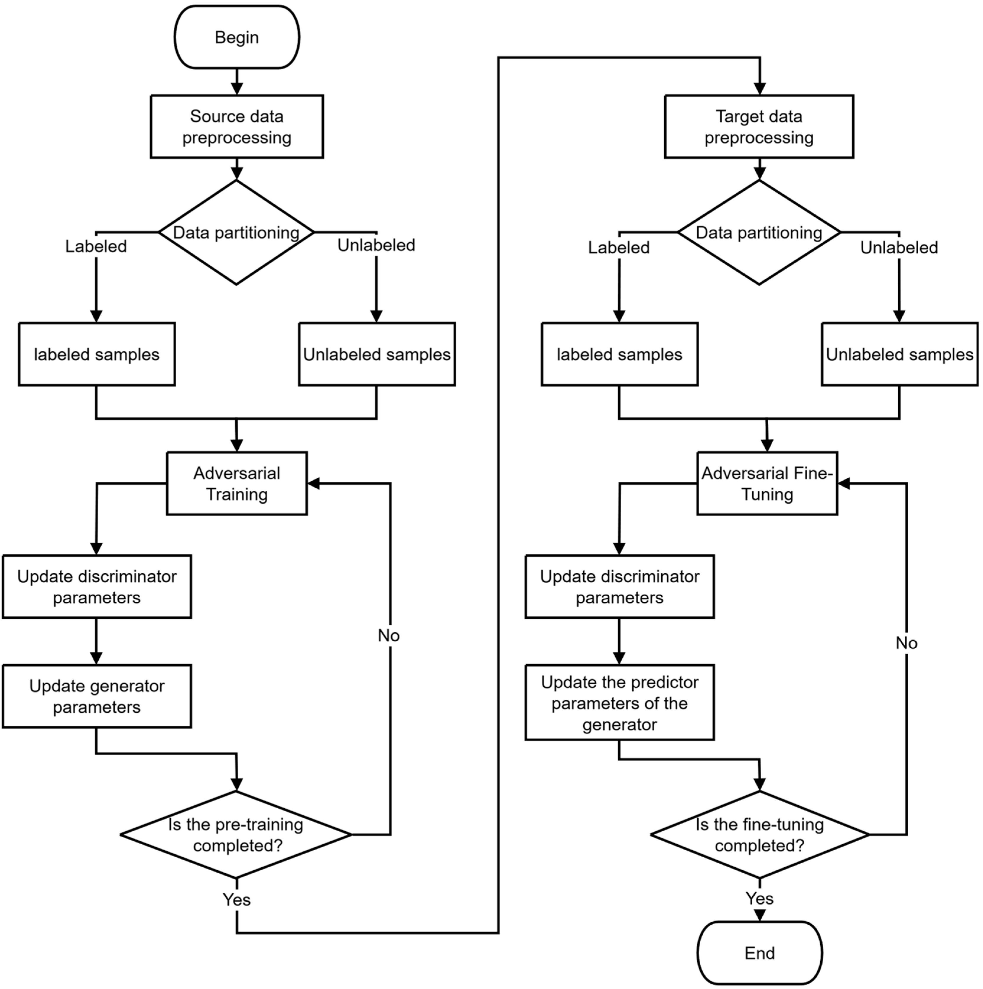
The adversarial semi-supervised pre-training fine-tuning strategy can be illustrated in Figure 3.

Figure 3. Flow diagram of the adversarial semi-supervised pre-training fine-tuning strategy.

3. Results and Discussion

3.1. Data Preprocessing

3.1.1. Data Cleaning

The purpose of data cleaning is to identify and correct (or remove) errors and inconsistencies in the dataset, including handling missing values and outliers. This process is crucial for enhancing the accuracy and reliability of the model.

In this study, the collected data from the sugar factory contains approximately 8.5% missing values, the majority of which are consecutive gaps resulting from seasonal operations and can thus be excluded from the analysis period. Therefore, samples containing NaN values, zeros, and non-numeric types were directly removed to mitigate the potential negative impact of missing values on the accuracy of model training.

To assess the potential presence of significant outliers in the dataset, an exploratory analysis was conducted using the K-means clustering algorithm. The algorithm was applied to partition the data into multiple clusters. The objective was to examine whether any clusters would emerge that were distinctly separate from the main data distribution, which could indicate anomalous subgroups. We followed common practice by analyzing the clustering performance for k values ranging from 2 to 10 using the elbow method, in order to determine the optimal number of clusters. A cluster was flagged as a potential anomalous subgroup if the Euclidean distance between its centroid and the centroid of the largest primary cluster exceeded three standard deviations above the mean (> μ + 3σ) of the pairwise distances between all cluster centroids. The results indicate that the clustering outcomes under different K-values did not yield any stable, extremely small isolated clusters. Instead, all data points were relatively evenly distributed among several primary clusters. Therefore, no samples were excluded based on this exploratory check.

3.1.2. Data Normalization

This study employs the min–max normalization method to scale the data to the [0, 1] range. The specific process of this method is as follows:

$$X’={\displaystyle \frac{X-X_{\min }}{X_{\max }-X_{\min }}}$$

(13)

where $X$ is the original data, $X_{\min }$ is the minimum value in the data, $X_{\max }$ is the maximum value in the data, and $X’$ is the normalized data. In this process, the training set is standardized independently, while the test set is standardized using the maximum and minimum values from the training set.

3.1.3. Constructing Coarse-Grained Data

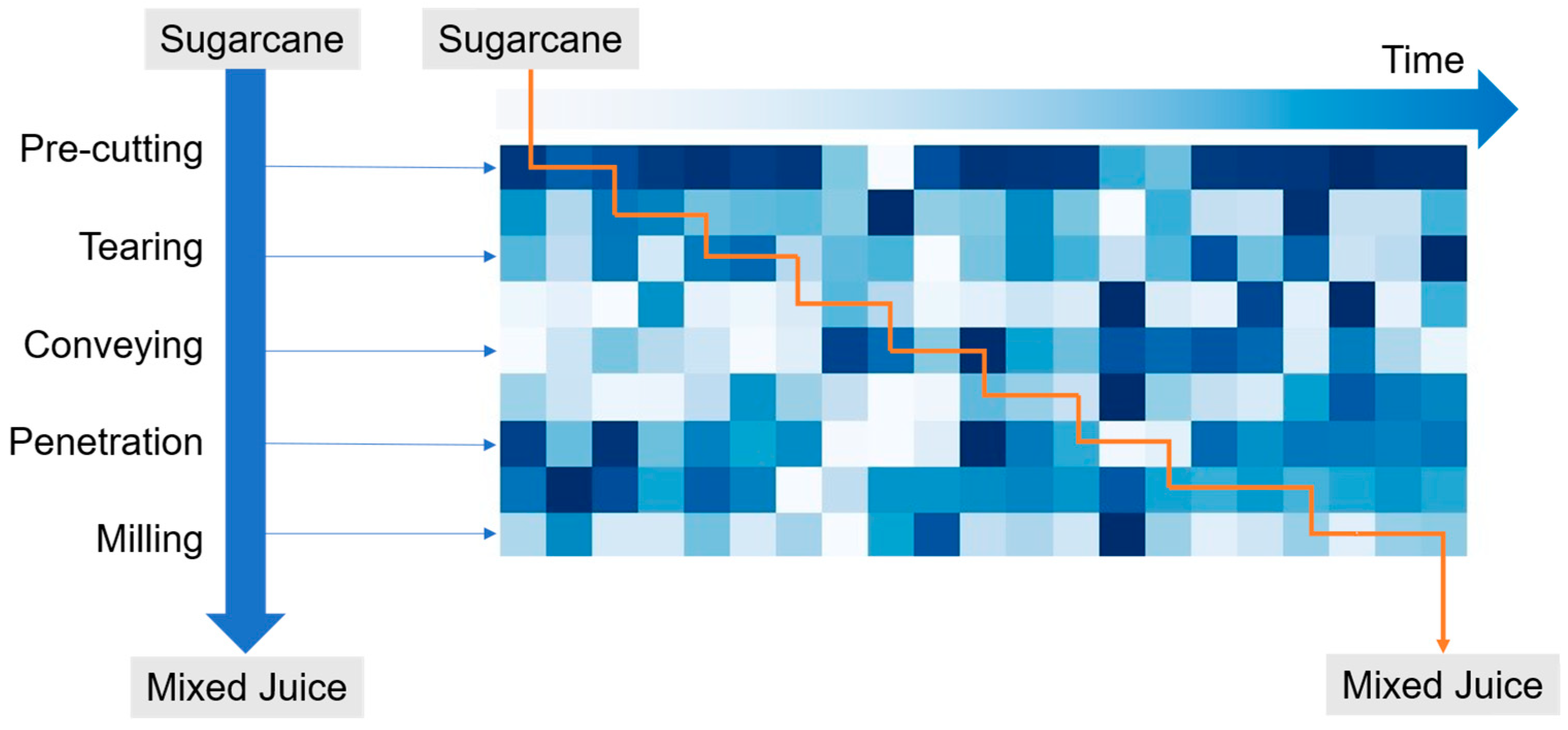
The sugarcane milling process, as a typical process industry, exhibits a chain reaction where early parameter variations affect subsequent stages, demonstrating a close temporal and spatial relationship between data and quality indicators. Therefore, this study establishes coarse-grained data for sugarcane milling to predict the initial juice sugar content (Figure 4) [21]. This data is presented in the form of grayscale images, where each pixel represents a parameter value, and the color intensity reflects the magnitude of the parameter. The horizontal and vertical axes represent time and the milling process, respectively, showcasing the spatiotemporal dynamic relationship between the process and quality.

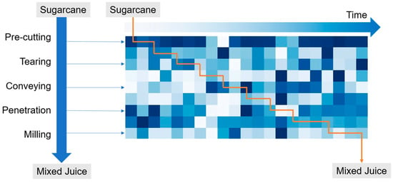
Figure 4. Schematic diagram of sugarcane milling coarse data.

The construction of the 9 × 21 × 1 coarse-grained data representation involves the following key steps:

Data Windowing: A sliding window approach is applied to the multivariate time series data of the milling process. The window length is set to 21 min, corresponding to the optimal historical time span determined for the input data. This window moves forward through the time series with a step size of one minute, capturing sequential snapshots of the process state.

Feature Selection and Alignment: For each 21 min window, data from nine key process parameters (e.g., feed rate, crusher torque, primary juice pH) are selected. These nine parameters correspond to the nine rows of the final image. The data points within the window for each parameter are aligned such that the most recent time point (time t) is positioned at the rightmost column, and the earliest point (t-20 min) is at the leftmost column. This creates a 9 (parameters) × 21 (time steps) matrix for each window.

Temporal Alignment with the Quality Label (No Intentional Lag): The quality indicator, the initial juice sugar content, is measured from the juice extracted at the end of the milling stage. Given the immediate physical relationship between the operational parameters (like crusher current) and the resulting juice quality, there is no significant time lag between the end of the data window and the quality measurement. Therefore, the 9 × 21 data matrix ending at time t is directly associated with (i.e., used to predict) the sugar content measured at the same time t (or effectively concurrently). This alignment reflects the near-real-time causality in the process.

Image Formation: The final 9 × 21 data matrix is normalized so that parameter values are scaled to a range of [0, 1]. Each normalized value is then treated as a pixel intensity, forming a 9 × 21 × 1 grayscale image, where the third dimension (1) signifies a single channel.

To determine the optimal time delay for input data, this study employed a Convolutional Neural Network (CNN) model to predict the initial juice sugar content under different time delay conditions. It was found that when the maximum time delay exceeded 21 min, the prediction performance no longer showed significant improvement. Therefore, this study established 21 min as the optimal time delay for input data, setting the size of each input sample to 9 × 21 × 1.

3.1.4. Data Distribution Adaptation

Due to the limited amount of data from the target production line and the potential shift in future data distribution over time, the current training data distribution may not fully reflect the characteristics of future test data distribution. This could lead to a decrease in the prediction accuracy of the fine-tuned model. Therefore, it is essential to adopt a data distribution adaptation strategy to ensure that the distributions of the training data and the test data become consistent.

The data processing method of Weighted Moving Average (WMA) was used [22], specifically:

(1)

During data processing, the weighted average of every adjacent m data points is taken, with higher weights assigned to closer time points and lower weights to more distant ones. This method reduces the time delay. The weighted average is:

$$WMA={\displaystyle \frac{{\displaystyle \sum _{i=1}^m{W}_i}\cdot X_{n-i+1}}{{\displaystyle \sum _{i=1}^m{W}_i}}}$$

(14)

Among them,

$X_{n-i+1}$ represents the value of the $(n-i+1)$ th data point in the sequence.

$n$ is the position of the data point currently under consideration.

$W_i$ is the weight of the $i$ th data point, specifically defined as

$$W_i={\alpha }^{m-i}$$

(15)

In this paper, $\alpha$ is set to 2, and $m$ is set to 10.

(2)

Using the residual data, which is obtained by subtracting the weighted moving average of the data from the initial data, as the training data for the model.

$$R_{\mathrm{t}}=X_{\mathrm{t}}-WM{A}_{\mathrm{t}}$$

(16)

(3)

When predicting future test data, to ensure the model focuses on learning the irregular fluctuations in the data, the weighted moving average of the previous data is used as the mean for the next data point.

After the aforementioned preprocessing methods, 190,000 samples from production line A were selected as source domain data, including 500 labels for pre-training model construction. Production line B used 10,000 real-time monitoring samples and 100 labels for fine-tuning training, with the remaining 500 labeled data used as the test set.

3.2. Model Structure and Hyperparameter Settings

This paper utilizes the CNN model as the foundational model. The feature extractor employs the Resnet network structure, which includes four residual units to further enhance feature extraction capabilities. Each residual unit uses a 3 × 3 convolutional kernel, with a stride of 1 and padding of 1, ensuring that the input and output dimensions remain the same. Between the residual units, a 3 × 3 convolutional kernel with a stride of 1 and no padding is used to reduce the feature map size. The channel numbers of the four residual units are 8, 16, 32, and 64, respectively. Finally, global average pooling is used to achieve feature flattening, resulting in a feature dimension of 1 × 64.

The regressor part employs a two-layer fully connected neural network with 128 and 32 nodes in each layer, respectively. The activation function for all layers of the model is LeakyReLU. Batch normalization is used during training to accelerate convergence, and the SGD optimizer is adopted to update the model parameters. The learning rate scheduler follows a fixed strategy, maintaining a constant learning rate throughout the training process. The network weight parameters are initialized using the Xavier method, while the bias parameters are set to 0.

Using the random search tuning method, hyperparameters for both the pre-training and fine-tuning processes were sequentially adjusted. For the fine-tuning part, five repeated experiments were conducted using different random seeds. The hyperparameters to be tuned and the tuning results are shown in Table 2.

Table 2. Hyperparameter tuning results for pre-training and fine-tuning processes.

Hyperparameters	Pre-Training	Fine-Tuning
Epochs	174	136
Generator learning rate	0.001	0.0005
Generator momentum	0.9	0
Discriminator learning rate	0.0001	0.01
Batch size of labeled data	500	50
Batch size of unlabeled data	200	200
Coefficient of the generator discrimination loss	50	100

3.3. Prediction Results and Analysis

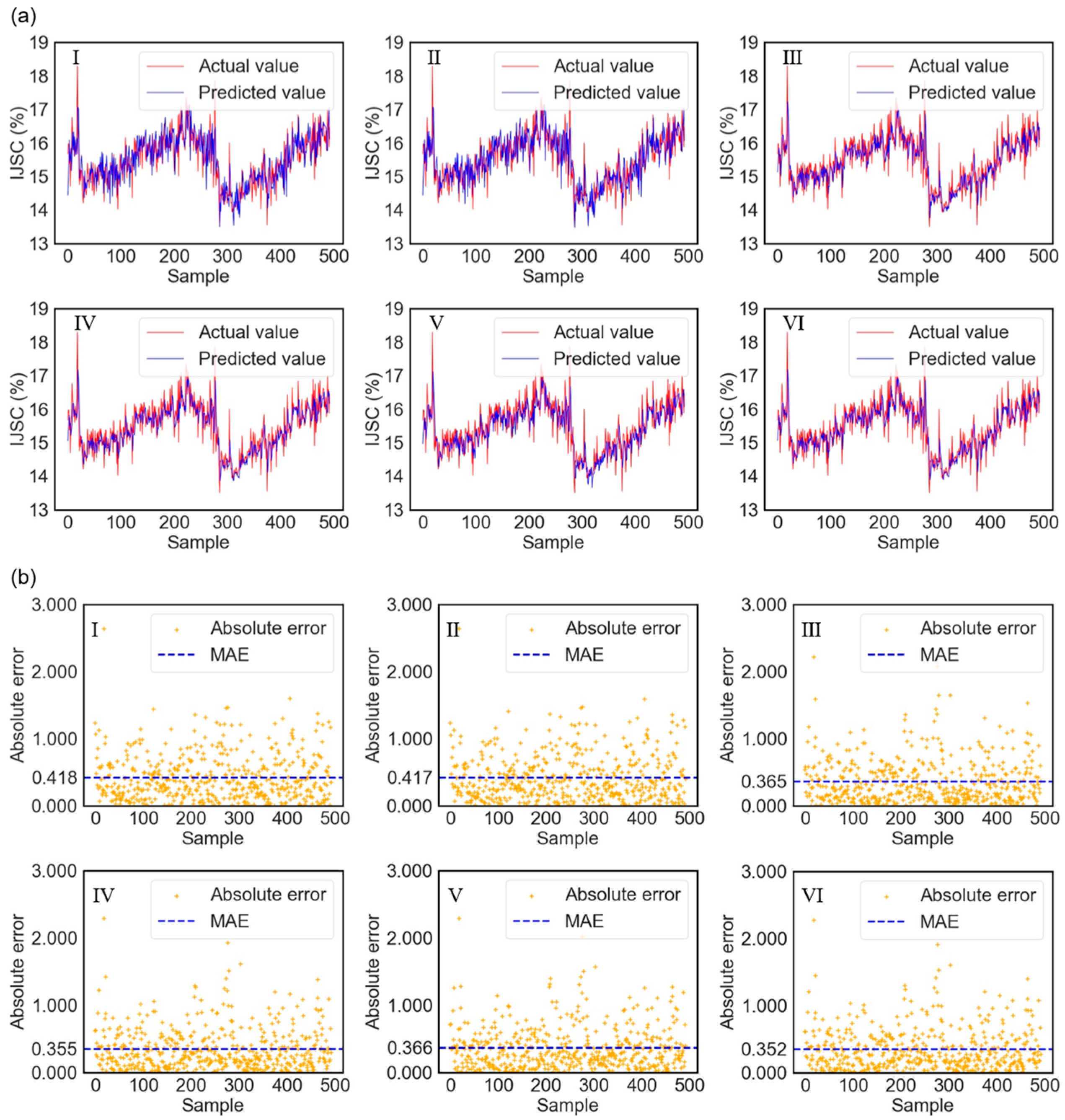
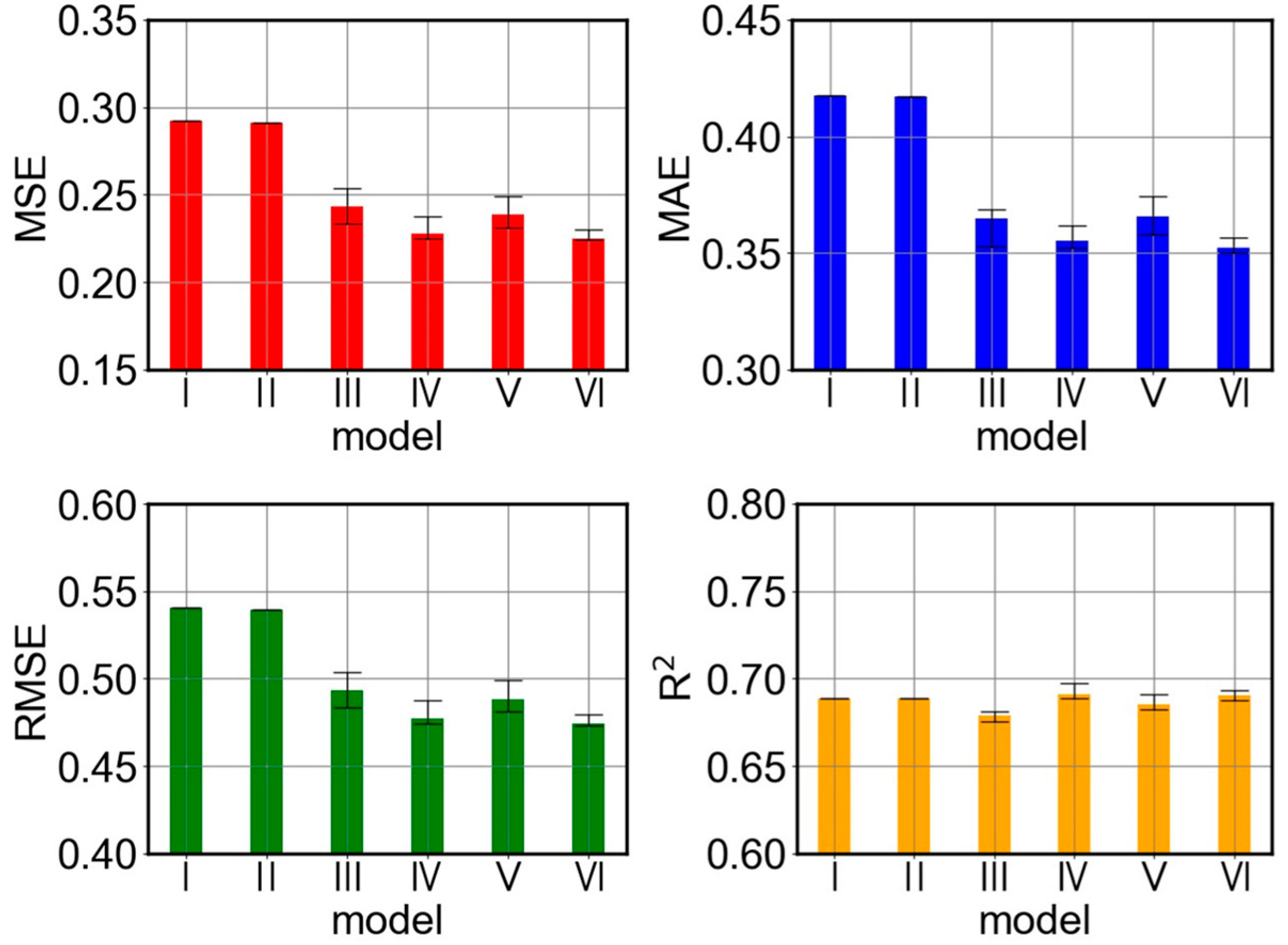
This study conducts an in-depth evaluation of the performance of adversarial semi-supervised pretraining and fine-tuning models, quantified through key metrics such as MSE, RMSE, MAE, and R². To verify the effectiveness of this strategy, a series of ablation experiments were conducted, comparing the predictive performance and metrics of six models: the ordinary pretraining model, the adversarial semi-supervised pretraining model, the adversarial semi-supervised fine-tuning model, the model using adversarial semi-supervised pretraining only during the pretraining phase, the model using adversarial semi-supervised pretraining only during the fine-tuning phase, and the complete adversarial semi-supervised pretraining and fine-tuning model. The predictive performance is shown in Figure 5, and the comparison of predictive metrics is illustrated in Figure 6 and Table 3.

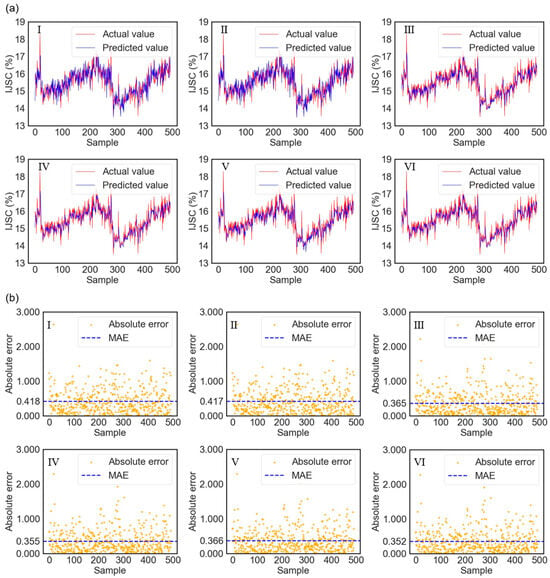
Figure 5. Performance comparison in predicting the initial juice sugar content among different models: (I) Standard pre-trained model. (II) Pre-trained model with adversarial semi-supervised learning. (III) Fine-tuned model with adversarial semi-supervised learning. (IV) Model fine-tuned with adversarial semi-supervised learning only during the pre-training phase. (V) Model fine-tuned with adversarial semi-supervised learning only during the fine-tuning phase. (VI) Complete adversarial semi-supervised pre-training fine-tuning: (a) Comparison between predicted values and actual values. (b) Absolute prediction error.

Figure 6. Comparison of metrics in predicting initial juice sugar content among different models: Conventional Pretraining Model (I). Pretraining Model using Adversarial Semi-supervised Learning (II). Finetuned Model using Adversarial Semi-supervised Learning (III). Model Finetuned with Adversarial Semi-supervised Pretraining only during the Pretraining Phase (IV). Model Finetuned with Adversarial Semi-supervised Pretraining only during the Finetuning Phase (V). Complete Adversarial Semi-supervised Pretraining and Finetuning (VI).

Table 3. Prediction metrics of models with different modeling strategies.

Model	MSE	RMSE	MAE	R2
Standard pre-trained model	0.292	0.541	0.418	0.689
Adversarial semi-supervised pre-trained model	0.291	0.539	0.417	0.689
Adversarial semi-supervised fine-tuned model	0.243 ± 0.00862	0.493 ± 0.00875	0.365 ± 0.00695	0.679 ± 0.00179
Fine-tuning without semi-supervised strategy	0.228 ± 0.00521	0.477 ± 0.00540	0.355 ± 0.00410	0.691 ± 0.00316
Pre-training without semi-supervised strategy	0.238 ± 0.00670	0.488 ± 0.00693	0.366 ± 0.00563	0.685 ± 0.00360
Complete adversarial semi-supervised pre-trained and fine-tuned model	0.225 ± 0.00201	0.474 ± 0.00209	0.352 ± 0.00177	0.690 ± 0.00181

The experimental results indicate that while the proposed complete model (VI) achieves the best performance in terms of MSE, RMSE, and MAE, the differences in R² values among the six models are minimal. This apparent inconsistency can be explained by the distinct statistical interpretations of these metrics. R² (coefficient of determination) primarily measures the proportion of the variance in the dependent variable that is predictable from the independent variables, reflecting the model’s goodness-of-fit to the overall data distribution. In contrast, MSE and MAE are absolute measures of error magnitude, more sensitive to the precise accuracy of individual predictions. In this industrial prediction task, the target variable (initial juice sugar content) likely has a relatively stable range under normal operating conditions. All compared models, being variants of the same underlying architecture, captured the main trends in the data, leading to similar R² values. However, the complete model (VI) achieved a significant reduction in prediction errors, lowering MSE by 23.0% and MAE by 15.7% compared to the standard pre-trained model (I). This superior precision in MSE and MAE indicates the model’s enhanced capability in minimizing larger prediction errors and achieving higher accuracy on a point-by-point basis, which is critical for practical process control. This superiority stems from the effective combination of pre-training, fine-tuning, and adversarial semi-supervised learning, which better handles the domain shift and leverages unlabeled data to refine the model’s predictions beyond just capturing the primary data trend.

Among the two models without fine-tuning, compared to the complete model, the conventional pre-trained model increased MSE, RMSE, and MAE by 0.06714, 0.06616, and 0.06568, respectively. For the pre-trained model using adversarial semi-supervised learning, these metrics improved by 0.06586, 0.06497, and 0.0651, respectively. The metrics for both models are significantly higher than those of the complete model, indicating that directly applying data-driven models from the source production line to the target production line will result in significant prediction bias, thus highlighting the crucial importance of fine-tuning. Although adversarial semi-supervised learning enhanced model performance during the pre-training phase, demonstrating its ability to improve model generalization, this improvement was still relatively limited. This suggests that merely incorporating adversarial semi-supervised learning in pre-training cannot fully bridge the gap between source and target domains.

In comparison, the fine-tuned models significantly outperform the non-fine-tuned models in prediction effectiveness. Under the same conditions of employing adversarial semi-supervised learning during the fine-tuning phase, the model without pre-training shows higher MSE, RMSE, and MAE values than the complete model by 0.01824, 0.01885, and 0.01268, respectively. Meanwhile, the model with only standard pre-training exhibits values in these three metrics that are 0.01342, 0.01395, and 0.01367 higher than the complete model. Overall, the model without pre-training performs poorly, highlighting the importance of pre-training. Furthermore, incorporating adversarial semi-supervised learning in the pre-training phase yields better results compared to standard pre-training, confirming the effectiveness of integrating adversarial semi-supervised strategies into the pre-training process.

When the semi-supervised learning strategy is not used during the fine-tuning stage, the model’s MSE, RMSE, and MAE are higher by 0.00263, 0.00277, and 0.00312, respectively, compared to the complete model. This indicates that using semi-supervised learning during the fine-tuning stage can improve the model’s prediction performance. However, this advantage is relatively limited, which could be because the model already possesses good generalization ability from the pre-training stage. The fine-tuning stage is primarily for adjusting the data distribution and does not require much additional information. Therefore, the benefits of using adversarial semi-supervised learning during fine-tuning are limited, and in practical applications, semi-supervised transfer learning can be applied during the fine-tuning stage as needed.

Since the R² values of the six model variants are relatively close, it is difficult to conclude that the proposed model achieves a significant performance improvement. Therefore, a Wilcoxon test was conducted between the proposed model and the other five models, with the test results presented in Table 4. All p-values are below 0.01, indicating that the proposed model achieves a statistically significant performance improvement.

Table 4. Wilcoxon Test Results of the Proposed Model and Model Variants.

Model Subjected to Wilcoxon Test with the Proposed Model	p-Value of the Wilcoxon Test
Standard pre-trained model	9.494 × 10−9
Adversarial semi-supervised pre-trained model	4.987 × 10−9
Adversarial semi-supervised fine-tuned model	0.000665
Fine-tuning without semi-supervised strategy	0.000907
Pre-training without semi-supervised strategy	0.0093

Overall, these analysis results confirm the effectiveness of pre-training fine-tuning and adversarial semi-supervised learning in improving the prediction accuracy of the model under the target production line. Among these, the importance of the fine-tuning stage is the most prominent, followed by the application of the pre-trained model, then the adversarial semi-supervised learning adopted during the pre-training process, while the benefits of applying adversarial semi-supervised learning during the fine-tuning process are relatively minor.

3.4. Effect of Label Quantity on Model Performance

The predictive performance of the adversarial semi-supervised pre-training fine-tuning model under conditions of insufficient label numbers was investigated by comparing the model’s predictive performance under different label quantities. Specifically, 190,000 unlabeled data points and 500 labeled data points from production line A were selected, and 10,000 unlabeled data points from production line B were used. Different quantities of labeled data from production line B were set to construct adversarial semi-supervised pre-training fine-tuning models to predict the initial juice sugar content of production line B. A fixed test set of 140 labeled samples from production line B was held out for evaluation. The remaining labeled data from production line B were used to create the training sets with different label quantities (250, 100, 50, 25, 10, 5, 3), ensuring no overlap between the training and test sets. Perform 5 repeated trials for each label quantity using different random seeds. The predictive performance of these models was evaluated using 140 labeled data points as the test set to explore the impact of label quantity on the predictive performance of the adversarial semi-supervised pre-training fine-tuning model. The predictive metrics of the initial juice sugar content under different label quantities for the adversarial semi-supervised pre-training fine-tuning models are shown in Figure 7 and Table 5.

Figure 7. Prediction metrics of the adversarial semi-supervised pre-training fine-tuning model under different numbers of labels.

Table 5. Predictive indicators of the adversarial semi-supervised pretraining fine-tuning model for predicting initial juice sugar content under different numbers of labels.

Number of Labels	MSE	MAE	R2
250	0.226 ± 0.00518	0.364 ± 0.00540	0.619 ± 0.00636
100	0.232 ± 0.0103	0.369 ± 0.00998	0.619 ± 0.00571
50	0.229 ± 0.0084	0.366 ± 0.00746	0.62 ± 0.00575
25	0.236 ± 0.00826	0.371 ± 0.00797	0.621 ± 0.00441
10	0.224 ± 0.00498	0.362 ± 0.00743	0.62 ± 0.00534
5	0.242 ± 0.0201	0.38 ± 0.023	0.619 ± 0.00408
3	0.249 ± 0.026	0.385 ± 0.0256	0.618 ± 0.00425

From Figure 7 and Table 5, it can be observed that when the number of labels ranges from 250 to 10, most of the MSE remains between 0.22 and 0.24, the MSE remains below 0.38, and the R² is above 0.6. The differences in various metrics are minimal, indicating that even when the number of labels is reduced to 10, the model can still maintain good predictive performance. When the number of labels falls below 10, the predictive performance starts to decline, but it still retains basic predictive accuracy. This suggests that the pre-trained model has strong generalization capabilities and can extract universal features for predicting initial juice sugar content. Even in cases where the target production line has very few labels, it can maintain a certain level of predictive performance.

These results demonstrate the high data efficiency of the adversarial semi-supervised pre-training fine-tuning framework. The key message is that the model’s performance remains stable and satisfactory even when the number of target domain labels is reduced to as low as 10. This indicates that the pre-training stage on the large source domain (Production Line A) successfully transfers universal feature representations, thereby drastically reducing the reliance on labeled data from the target domain (Production Line B).

However, it is important to clarify the limitations of this data efficiency. The stability of performance plateaus when the number of labels is between 250 and 10, suggesting a lower practical bound for our specific task. When the labeled data is extremely scarce (fewer than 10 samples), the performance begins to degrade, indicating that a minimal amount of target-domain supervision is still indispensable for effective domain adaptation. Therefore, while the model is highly data-efficient, it is not completely data-agnostic.

4. Conclusions

A transfer learning strategy is proposed in this paper, which combines adversarial semi-supervised learning and pre-training fine-tuning to address the issue of cross-production line data-driven model transfer under the condition of scarce labeled data in two domains during sugarcane milling. The strategy first utilizes unlabeled data and a small amount of labeled data from the source production line during the pre-training stage to train the model’s feature extractor and classifier through adversarial semi-supervised learning. Then, during the fine-tuning stage, only the predictor part of the model is trained to adapt to the data distribution of the target production line.

The effectiveness of the proposed prediction strategy was verified through ablation experiments. The results demonstrated that the adversarial semi-supervised pre-training and fine-tuning method has significant advantages in predicting the initial juice sugar content of the target production line. Specifically, our complete model achieved the best performance, reducing the Mean Squared Error (MSE) by approximately 23.0% and the Mean Absolute Error (MAE) by approximately 15.7% compared to the standard pre-trained model without fine-tuning. Both pre-training fine-tuning and adversarial semi-supervised learning were effective in improving the model’s prediction accuracy on the target production line. Among these, the fine-tuning phase was the most important, followed by the pre-trained model, then the adversarial semi-supervised training in pre-training, while the adversarial semi-supervised training in fine-tuning showed the smallest advantage. The model maintained good prediction performance when the number of labels was greater than 10. When the number of labels was less than 10, the prediction performance began to decline but still maintained a certain level of predictive ability.

However, this study still has limitations. First, the validation was conducted on production lines within the same region. The model’s effectiveness across different geographical regions with varying sugarcane varieties and practices requires further investigation. Second, while our method handles covariate shift, it assumes consistent process parameters across lines. Transfer learning between lines with heterogeneous parameters remains a challenge for future work.

Future research can be further expanded in the following directions:

(1)

The number and types of process parameters vary across different production lines, and it is of significant importance to study how to enable data-driven models to transfer between production lines with different parameters.

(2)

Collect more environmental data, sugarcane condition data, and mechanical assembly data to more accurately predict the quality indicators of sugarcane milling.

References

- Oktarini, D.; Mohruni, A.S.; Sharif, S.; Yanis, M.; Madagaskar. Optimum milling parameters of sugarcane juice production using Artificial Neural Networks (ANN). J. Phys. Conf. Ser. 2019, 1167, 012016. [Google Scholar] [CrossRef]
- Meng, Y.; Chen, J.; Li, Z.; Zhang, Y.; Liang, L.; Zhu, J. Soft sensor with deep feature extraction for a sugarcane milling system. J. Food Process Eng. 2022, 45, e14066. [Google Scholar] [CrossRef]
- Li, Z.; Chen, J.; Meng, Y.; Zhu, J.; Li, J.; Zhang, Y.; Li, C. Multi-objective optimization of sugarcane milling system operations based on a deep data-driven model. Foods 2022, 11, 3845. [Google Scholar] [CrossRef] [PubMed]
- Qiu, M.; Meng, Y.; Chen, J.; Chen, Y.; Li, Z.; Li, J. Dual multi-objective optimisation of the cane milling process. Comput. Ind. Eng. 2023, 179, 109146. [Google Scholar] [CrossRef]
- Yang, T.; Mao, H.; Yin, Y.; Zhong, J.; Wen, J.; Ding, J.; Duan, Q. Hybrid data-driven modeling for accurate prediction of quality parameters in sugarcane milling with fine-tuning. J. Food Process Eng. 2023, 46, e14436. [Google Scholar] [CrossRef]
- Li, C.; Liu, Y.; Meng, Y.; Duan, Q. Sugarcane juice extraction prediction with Physical Informed Neural Networks. J. Food Eng. 2024, 364, 111774. [Google Scholar] [CrossRef]
- Xu, K.; Li, Y.; Liu, C.; Liu, X.; Hao, X.; Gao, J.; Maropoulos, P.G. Advanced Data Collection and Analysis in Data-Driven Manufacturing Process. Chin. J. Mech. Eng. (Engl. Ed.) 2020, 33, 1–21. [Google Scholar] [CrossRef]
- Fisher, O.J.; Watson, N.J.; Escrig, J.E.; Witt, R.; Porcu, L.; Bacon, D.; Rigley, M.; Gomes, R.L. Considerations, challenges and opportunities when developing data-driven models for process manufacturing systems. Comput. Chem. Eng. 2020, 140, 106881. [Google Scholar] [CrossRef]
- Yosinski, J.; Clune, J.; Bengio, Y.; Lipson, H. How transferable are features in deep neural networks? Adv. Neural Inf. Process. Syst. 2014, 27, 3320–3328. [Google Scholar] [CrossRef]
- Wang, H.; Liu, M.; Shen, W. Industrial-generative pre-trained transformer for intelligent manufacturing systems. IET Coll. Intel. Manuf. 2023, 5, e12078. [Google Scholar] [CrossRef]
- Wu, Y.; Liu, D.; Yuan, X.; Wang, Y. A just-in-time fine-tuning framework for deep learning of SAE in adaptive data-driven modeling of time-varying industrial processes. IEEE Sens. J. 2020, 21, 3497–3505. [Google Scholar] [CrossRef]
- Yesilbas, D.; Arnold, S.; Felker, A. Rethinking Pre-Training in Industrial Quality Control. In Proceedings of the 17th International Conference on Wirtschaftsinformatik, Nuremberg, Germany, 21–23 February 2022; Available online: https://aisel.aisnet.org/wi2022/analytics_talks/analytics_talks/2 (accessed on 14 March 2022).
- Yuan, H.; Yuan, Z.; Yu, S. Generative biomedical entity linking via knowledge base-guided pre-training and synonyms-aware fine-tuning. In Proceedings of the 2022 Conference of the North American Chapter of the Association for Computational Linguistics: Human Language Technologies, Seattle, WA, USA, 10–15 July 2022; pp. 4038–4048. [Google Scholar] [CrossRef]
- Yarowsky, D. Unsupervised word sense disambiguation rivaling supervised methods. In Proceedings of the 33rd Annual Meeting of the Association for Computational Linguistics, Cambridge, MA, USA, 26–30 June 1995; pp. 189–196. [Google Scholar] [CrossRef]
- Goodfellow, I.; Pouget-Abadie, J.; Mirza, M.; Xu, B.; Warde-Farley, D.; Ozair, S.; Courville, A.; Bengio, Y. Generative adversarial nets. In Proceedings of the 28th International Conference on Neural Information Processing Systems, Montreal, QC, Canada, 8–13 December 2014; Volume 2, pp. 2672–2680. Available online: https://dl.acm.org/doi/10.5555/2969033.2969125 (accessed on 14 March 2022).
- Akhyar, F.; Furqon, E.N.; Lin, C.Y. Enhancing Precision with an Ensemble Generative Adversarial Network for Steel Surface Defect Detectors (EnsGAN-SDD). Sensors 2022, 22, 4257. [Google Scholar] [CrossRef] [PubMed]
- Qian, C.; Yu, W.; Lu, C.; Griffith, D.; Golmie, N. Toward generative adversarial networks for the industrial internet of things. IEEE Internet Things J. 2022, 9, 19147–19159. [Google Scholar] [CrossRef]
- Wang, A.; Zhang, S.; Chen, C.; Zheng, Z. P-4.10: Simulation Algorithm of Industrial Defects based on Generative Adversarial Network. Int. Conf. Disp. Technol. (ICDT 2020) 2021, 52, 510–513. [Google Scholar] [CrossRef]
- Abuduweili, A.; Li, X.; Shi, H.; Xu, C.-Z.; Dou, D. Adaptive consistency regularization for semi-supervised transfer learning. In Proceedings of the IEEE/CVF Conference on Computer Vision and Pattern Recognition, Nashville, TN, USA, 20–25 June 2021; pp. 6923–6932. [Google Scholar] [CrossRef]
- Sun, X.; Qiao, Y. Fake comments identification based on symbiotic articulation oftransfer learning and semi-supervised learning. J. Nanjing Univ. (Nat. Sci.) 2022, 58, 846–855. [Google Scholar] [CrossRef]
- Jiang, X.; Ge, Z. Augmented multidimensional convolutional neural network for industrial soft sensing. IEEE Trans. Instrum. Meas. 2021, 70, 1–10. [Google Scholar] [CrossRef]
- Perry, M.B. The Weighted Moving Average Technique. In Wiley Encyclopedia of Operations Research and Management Science; Wiley: Hoboken, NJ, USA, 2011. [Google Scholar] [CrossRef]
Disclaimer/Publisher’s Note: The statements, opinions and data contained in all publications are solely those of the individual author(s) and contributor(s) and not of MDPI and/or the editor(s). MDPI and/or the editor(s) disclaim responsibility for any injury to people or property resulting from any ideas, methods, instructions or products referred to in the content. |
© 2025 by the authors. Licensee MDPI, Basel, Switzerland. This article is an open access article distributed under the terms and conditions of the Creative Commons Attribution (CC BY) license (https://creativecommons.org/licenses/by/4.0/).