Abstract
To address the pressing challenges of low new energy utilization, high power system operating costs, and compromised power supply reliability in regional grids, we propose a multi-time-scale source–storage–load coordinated scheduling strategy that explicitly accounts for the characteristic distribution of grid-connected energy storage stations, including their state-of-charge constraints, round-trip efficiency profiles, and location-specific operational dynamics. A day-ahead scheduling framework is developed by integrating the multi-time-scale behavioral patterns of diverse load-side demand response resources with the dynamic operational characteristics of energy storage stations. By embedding intra-day rolling optimization and real-time corrective adjustments, we mitigate prediction errors and adapt to unforeseen system disturbances, ensuring enhanced operational accuracy. The objective function minimizes a weighted sum of system operation costs encompassing generation, transmission, and auxiliary services; wind power curtailment penalties for unused renewables; and load shedding penalties from unmet demand, balancing economic efficiency with supply quality. A mixed-integer programming model formalizes these tradeoffs, solved via MATLAB 2020b coupled CPLEX to guarantee optimality. Simulation results demonstrate that the strategy significantly cuts wind power curtailment, reduces system costs, and elevates new energy consumption—outperforming conventional single-time-scale methods in harmonizing renewable integration with grid reliability. This work offers a practical solution for enhancing grid flexibility in high-renewable penetration scenarios.
1. Introduction
As of the end of 2024, China’s installed wind power capacity reached 520 GW (up 18% year-on-year), and photovoltaic (PV) capacity hit 890 GW (up 45.2% year-on-year) [1], ranking first globally in both metrics. However, this rapid renewable expansion has exacerbated curtailment challenges; regional wind and solar curtailment rates hovered above 20% in 2024 [2], underscoring the urgent need to enhance grid flexibility for new energy accommodation. The evolution of global installed power capacity by source and the proportion of new energy is shown in Figure 1.
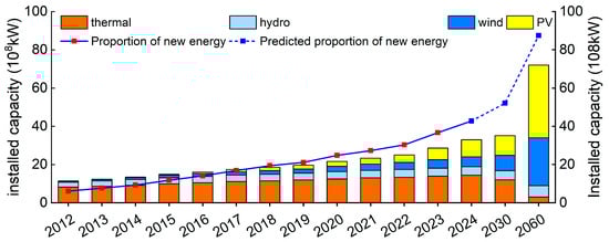
Figure 1.
Evolution of global installed power capacity by source and the proportion of new energy.
To address this, China has prioritized energy storage deployment, driving the evolution of power systems from traditional “source–grid–load” frameworks to integrated “source–grid–load–storage” architectures. Notable demonstrations include Jiangsu’s Jianshan Energy Storage Station and Nanjing’s Jiangbei Energy Storage Station—both electrochemical projects equipped with smart “source–grid–load” interactive terminals. These facilities have not only enabled seamless integration with regional grids but also boosted new energy consumption by 12–15% in Jiangsu, validating the efficacy of storage-enabled coordination [3].
With the transition towards active distribution networks—characterized by active control, services, and management—the integrated scheduling of diverse grid assets (including distributed energy resources, storage devices, and responsive loads) has become feasible. However, while studies on fundamental complementarity (e.g., “source–load” and “grid–load–storage” [4,5]) are mature, research on holistic “source–grid–load–storage” cooperative scheduling is still lacking.
To address the coordination challenges in power grids, a diverse set of methodological approaches has been developed within theoretical research on the optimal scheduling of integrated energy systems. Literature [6] employs the Lagrange multiplier method to collaboratively optimize individual schedulable resources within localized energy networks—while this approach excels in local resource allocation precision, it may struggle to ensure global convergence. Literature [7] uses artificial intelligence algorithms to holistically optimize global performance indicators for source–network–load–storage systems, though such AI-driven methods often face issues of poor interpretability and heavy computational burden. Literature [8] develops a distributed algorithm-based solution for collaborative optimization models, achieving faster computation speeds and improved convergence—critical advantages for large-scale grid operations. Literature [9] proposes an energy router-based strategy to optimize the management of individual schedulable resources, enhancing flexibility at the distribution level. Literature [10] presents a three-layer grid planning model and solves the collaborative optimization problem using a hybrid algorithm combining support vector regression (SVR)—a technique with strong global search capabilities—and a parallel genetic membrane algorithm (PGMA). These studies have collectively advanced the field, yet many still grapple with balancing computational efficiency, scalability, and real-world adaptability in complex, high-renewable-penetration environments. Literature [11] proposed a two-stage stochastic robust optimization method for campus integrated energy systems accounting for uncertainties in new energy and load. Literature [12], considering uncertainty in hydrogen prices, put forward a shared energy storage framework incorporating hydrogen trading for campus, industrial, and commercial integrated energy systems. It designed a hierarchical optimal scheduling method based on Stackelberg game relationships and conducted case studies using an algorithm combining Particle Swarm Optimization (PSO) and Mixed-Integer Linear Programming (MILP), verifying the rationality of electric–hydrogen shared energy storage. Literature [13] addressed uncertainty in wind and photovoltaic output by proposing a multi-source cooperative game robust optimization scheduling model for wind-solar-storage systems that accounts for fairness. Literature [14] established a Stackelberg game-based hybrid energy sharing mechanism for integrated energy systems considering load uncertainty, where the integrated energy system operator acts as the leader and prosumers as followers. This mechanism simultaneously optimizes the leader’s upper-level profit and the followers’ lower-level energy usage efficiency.
The above-mentioned literature proposed innovations from the perspectives of a unified energy management system, hierarchical planning of the collaborative model, and the rapid search capabilities of the solution algorithm. By establishing a “source–grid–load–storage” collaborative scheduling model and formulating the day-ahead scheduling plan, the capacity of the power grid to accommodate new energy was improved. However, there are the following overlooked aspects: (1) The volatility and randomness of new energy output, and the uncertainty of demand response loads can affect the accuracy of the day-ahead scheduling plan formulated by the power grid. (2) Engineering practice shows that electrochemical energy storage is the current development trend of energy storage stations, while pumped storage power stations remain the main energy storage method. However, electrochemical energy storage has different output characteristics from traditional pumped storage power stations, and there are few relevant studies comparing the output characteristics of the two types of energy storage stations. (3) The research on the “source–grid–load–storage” scheduling model only considers the day-ahead scheduling situation of the power grid, while ignoring the emergency mode of the power grid, which is not conducive to the stability of the long-term operation of the power grid. The emergency modes are technically operationalized through a penalty-based mechanism within the objective function of our day-ahead scheduling model.
In order to address the aforementioned several issues, this paper adopts a stochastic programming multi-time-scale scheduling model based on scenario (scenario-based stochastic programming, SSP) and chance-constrained programming (CCP) [15,16] to revise the day-ahead scheduling plan and improve its accuracy The proposed method offers a simplified implementation structure while maintaining competitive performance, which could be advantageous for scenarios requiring rapid deployment or where computational resources are a primary concern compared to some complex multi-timescale strategies. By comparing the energy storage characteristics of the two types of energy storage power stations and comprehensively considering the time-scale characteristics of conventional units, wind turbines, energy storage power stations, and demand response loads, a multi-time-scale “source–grid–load–storage” scheduling model is established. Furthermore, adding the objective function of the emergency model in the scheduling model improves the power supply reliability of the grid in emergency mode. The model is solved using MATLAB 2020b coupled CPLEX, and the effect of the model is verified through practical examples.
2. The Operational Characteristics of Energy Storage Stations
Hydroelectric pumped storage offers rapid startup and large capacity but is constrained by geographical factors. In contrast, while other storage technologies like electrochemical systems provide siting flexibility and fast response, they face challenges of high costs and limited capacity. This study therefore focuses on analyzing pumped storage alongside the prevalent electrochemical energy storage technology.
2.1. Pumped Storage Energy Station
The operational cycle of a pumped storage plant—involving energy storage during low demand by pumping water to an upper reservoir and generation during peak demand—facilitates the conversion between electrical and mechanical energy. While the electromechanical process of generation, driven by the water turbine and generator, is identical to conventional hydropower, this also means its scheduling response is governed by the same mechanical inertia, thus lacking the ultra-fast regulation capability of power–electronic-based storage technologies.
2.2. Electrochemical Energy Storage Station
The principle of electrochemical energy storage, encompassing battery and supercapacitor technologies, is based on the reversible conversion between electrical and chemical energy. These systems are characterized by a high overall (round-trip) efficiency, typically ranging from 85% to 90%. Electrochemical energy storage technology is different from conventional units. It has a faster response speed and flexible scheduling capability, and its energy density is very high, allowing it to store a large amount of electrical energy. Electrochemical energy storage technology can better smooth out the output fluctuations of distributed power sources, promote system absorption, and has technical advantages such as strong environmental adaptability, capable of small-scale decentralized configuration, and short construction period [17].
3. Classification of Demand Response Resources
Load-side demand response resources (demand response, DR) are classified into two types based on the different response methods of users: price-based demand response (PDR) and incentive-based demand response (IDR) [17,18,19]. Among them, PDR can change users’ electricity usage patterns by implementing different price strategies, such as time-of-use pricing (TOU), real-time pricing (RTP), and critical peak pricing (CPP), etc.; IDR refers to the DR implementation agency formulating preferential policies to motivate users to respond to the scheduling signals. It mainly includes direct load control (DLC), interruptible load (IL), demand side bidding (DSB), and emergency demand response (EDR). Common examples in daily life include smart appliances and smart buildings.
In the model of this article, the electricity price adopts a dynamic day-ahead pricing model, so PDR needs to be determined in the day-ahead scheduling. And IDR can be classified into the following types based on the duration of responding to the grid scheduling instructions:
- (1)
- Type A IDR, which is planned 1 day in advance.
- (2)
- Type B IDR, with response duration ranging from 15 min to 2 h.
- (3)
- Type C IDR, with response duration ranging from 5 min to 15 min.
- (4)
- Type D IDR, which makes real-time responses.
4. Consider the Multi-Time-Scale Scheduling Plan for the Integration of Energy Storage Stations
The multi-time-scale scheduling framework for “source–storage–load” involving two types of energy storage stations, designed in this paper, is shown in Figure 2.

Figure 2.
Multi-time-scale scheduling framework.
- (1)
- The time scale of the day-ahead scheduling plan is 1 h, and the execution period is 24 h. In the day-ahead scheduling, it is necessary to determine the start–stop plans of conventional units, the charging and discharging electricity of pumped storage energy stations, the PDR load response volume, and the load calling plans of type A IDR. These are then used as determined quantities and substituted into the intra-day rolling optimization.
- (2)
- The intra-day optimization runs on a 4 h cycle. At the start of each cycle, the model calculates an optimal schedule for the upcoming period, with the timeline subdivided into 15 min time steps for detailed decision-making. In the intra-day scheduling, it is necessary to formulate the output plans of various new energy units, the charging and discharging electricity of electrochemical energy storage stations, and the calling plans of type B IDR loads. These are used to correct the deviations between the day-ahead scheduling plan and the actual situation. Among them, the start–stop plans and storage station plans of each unit and the load calling volume specified in the day-ahead scheduling plan remain unchanged.
- (3)
- The execution period of real-time coordinated control is 5 min. Its function is to use the intra-day rolling curve as a reference and conduct real-time coordinated control of the scheduling strategy to correct the actual working conditions and reduce deviations.
5. Multi-Time-Scale Coordinated Scheduling Model
5.1. The Day-Ahead Scheduling Optimization Model
Based on existing research, the day-ahead scheduling adopts a multi-scenario stochastic programming method suitable for high uncertainty [15], which can accommodate the errors in different load and new energy output prediction scenarios and meet the system safety constraints.
5.1.1. Objective Function
The objective function of the day-ahead scheduling model is formulated to minimize the total system operating cost, which includes the depreciation cost of electrochemical energy storage as well as penalty costs for wind curtailment and load shortage. This approach achieves a balanced optimization of economic efficiency, renewable energy integration, and power supply reliability, particularly during emergency operating modes.
In the formula: represents the objective function of the real-time scheduling optimization model, indicating the system operation cost; , , , and respectively represent the cost functions of conventional power plants, energy storage stations (including pumped storage and electrochemical storage), distributed energy plants, and user loads; represents the number of scenarios; is the probability coefficient for the occurrence of the s-th scenario; is the number of conventional power plants; is the power generation of the i-th conventional power plant at time t in the s-th scenario. , , and are the power generation cost coefficients of the i-th conventional unit; is the start–stop cost coefficient of the i-th conventional unit; represents the start–stop status of the i-th conventional unit at time t; and 1 indicates startup and 0 indicates shutdown; is the number of energy storage stations; is the number of electrochemical energy storage units; is the output power of energy storage station i at time t in the s scenario; is the cost function of the energy storage station; is the maintenance cost function of the energy storage station; represents the unit-time depreciation cost coefficient of electrochemical energy storage; represents the start–stop status of energy storage station i at time t; represents the number of distributed new energy units; PDGi,t,s represents the output of the i-th distributed unit at time t in the s scenario; represents the cost function of the distributed unit at time t in the s scenario; is the start–stop status of the distributed unit; represents the penalty cost coefficient for wind (solar) power rejection. represent the forecast output of distributed energy in scenario s at time t; and are the cost coefficients of type A and type B IDR, respectively; is the usage amount of type A IDR at time t; is the usage amount of type B IDR at time t in scenario s; is the penalty coefficient for load outage; and is the loss of load power at time t in scenario s.
5.1.2. Conventional Constraints
- (1)
- Power balance constraint conditions
In the formula: represents the part of the load that does not change with the electricity price; is the change in PDR load at time t; is the change in A IDR load at time t; and is the change in B IDR load at time t under scenario s.
- (2)
- Conventional unit operation constraints.
- (1)
- Unit output constraint conditions.
In the formula, and represent the upper and lower limits of the output of the i-th conventional unit, respectively.
- (2)
- The climbing slope constraint conditions for the aircraft.
In the formula, represents the climbing rate of the i-th conventional unit.
- (3)
- Constraints on distributed new energy output.
The output of new energy power generation should be less than the forecast value.
- (4)
- Operating constraints of energy storage stations.
- (1)
- Constraints of pumped storage energy storage power stations.
The constraints of pumped storage power stations mainly include the constraint of the reservoir’s capacity and the constraint of the climbing rate affected by the pumping rate.
In the formula: and , respectively represent the upper and lower limits of the grid-connected power of the pumping hydroelectric power station; and represent the upper and lower limits of the storage water volume of the pumped storage power station; represents the ramp rate of the pumped storage power station.
- (2)
- Constraints of electrochemical energy storage power station.
Electrochemical energy storage is mainly constrained by the rated power of the inverter and the rated charging and discharging power of the energy storage station.
In the formula: and represent the rated charging power and rated discharging power of the inverter, respectively; is the state of charge of the energy storage system; upper and lower limits; and and are the upper and lower limits of the state of charge of the energy storage system.
- (5)
- Power transmission constraint of the transmission line.
In the formula: represents the maximum transmission power between nodes ij; is the admittance between nodes ij; and represents the phase angle of node i in scenario s at time t.
- (6)
- Adjustment of each scene and constraint adjustment.
In the formula: and represent the base-load output values of conventional power plants and energy storage stations, respectively; and and represent the flexible scheduling capabilities of conventional power plants and energy storage stations, respectively.
- (7)
- Constraints of various DR resources.
In the formula: and represent the lower and upper limits of the load adjustment amount of PDR; and represent the increased load amounts of type A and type B IDR, respectively; and and represent the reduced load amounts of type A and type B IDR, respectively.
5.1.3. Optimized Result
By optimizing the algorithm to solve the day-ahead scheduling model, the following will be included as determining conditions and substituted into the subsequent day-ahead and real-time coordinated scheduling model: (1) the start–stop status of conventional units; (2) the charging and discharging power of pumped storage units; (3) the PDR scheduling volume, and the A IDR scheduling volume.
5.2. The Intra-Day Rolling Scheduling Optimization Model
The intra-day rolling optimization scheduling typically involves feeding the currently measured system data into the intra-day rolling optimization model, and then using the forecast data of wind and solar power loads over the next 4 h (with a time scale of 15 min) to solve for the optimal control sequence.
5.2.1. Objective Function
The objective function of the intra-day rolling optimization is also to minimize the system operation cost. Compared with the day-ahead scheduling model, in the rolling model, only the cost of the adjustment volume of IDR-type loads is changed. Since type A has been determined, the total load cost is the sum of type B and type C IDR. , , are the same as above.
In the formula: represents the cost coefficient of type C IDR; and is the traffic volume of type C IDR in the s scenario at time t.
5.2.2. Constraint Condition
Since the intra-day rolling model also employs the multi-scenario stochastic programming method to mitigate the adverse effects brought by uncertainties, its constraint conditions are basically the same as those in the day-ahead scheduling model. One additional constraint condition for type C IDR is included. This will not be repeated here.
5.2.3. Optimized Result
On the basis that the day-ahead scheduling has already determined the start–stop statuses of conventional generating units, the charging and discharging volumes of pumped storage units, the call volumes of PDR (Peak Demand Response), and the call volumes of type A IDR (Incentive-Based Demand Response) (which are set as known values and substituted into the calculations), the intra-day scheduling is conducted., ultimately determine:
- (1)
- The start–stop plan for distributed new energy units.
- (2)
- The charging and discharging capacity of the electrochemical energy storage station.
- (3)
- The load scheduling volume of B IDR.
5.3. The Real-Time Scheduling Model
Since the real-time scheduling time scale is 5 min, the robustness requirement for the scheduling decision quantity is higher. The multi-scenario stochastic planning method applicable to day-ahead scheduling and intra-day rolling models is no longer applicable. This paper adopts the chance-constraint method in the mathematical model. By setting certain constraints, the probability that the constraints hold is not less than a certain confidence level. The scenarios for the stochastic optimization were generated using the K-means clustering technique. The description includes key steps, such as:
Generating a large number of initial scenarios (1000) via Monte Carlo simulation based on the historical forecast error distributions of wind power and load.
Applying the K-means algorithm to reduce this large set to a limited number of representative scenarios (10) that capture the underlying probability distribution.
Calculating the probability for each representative scenario based on the number of original scenarios in its cluster.
5.3.1. Objective Function
For the real-time coordinated scheduling model, since it adopts the chance-constraint method and sets the constraint conditions for reserve capacity, the constraint conditions are smaller than the confidence level, thereby determining the rotational reserve capacity required by the system.
In the formula: represents the rotational standby cost of the system; , , and are the rotational standby cost coefficients for conventional units, distributed units, and pumped storage energy storage, respectively; and represent the positive and negative rotational standbys of conventional units; and and represent the positive and negative rotational standbys of pumped storage energy storage stations.
5.3.2. Constraint Condition
The intra-day scheduling determined the start–stop status of conventional units, PDR and type A IDR, as well as the scheduling volume of pumped storage energy storage stations. The intra-day rolling determined the start–stop status of distributed units, type B IDR and the scheduling volume of electrochemical energy storage stations. Therefore, only the power balance constraints, type C and type D IDR constraints, and reserve capacity constraints remain. The system constraints and IDR constraints are basically the same as before, and will not be elaborated on in this section. The main focus is on the reserve capacity constraints.
In the formula: Pr{} represents the confidence expression; and and are the confidence levels for positive rotational reserve capacity and negative rotational reserve capacity, respectively, and their values are 0.95.
5.3.3. Optimized Result
Optimizing the real-time scheduling model enables the determination of the following optimized results:
- (1)
- The start–stop status and output of all generating units.
- (2)
- The rotational reserve capacity.
- (3)
- The adjustment amounts of type C IDR and type D IDR.
6. Analysis of Examples
6.1. Example Introduction
In order to effectively address the serious issue of limited new energy consumption, this paper investigated a certain regional power grid in the East China region where new energy consumption was severely restricted. This grid was selected as a case study to verify the proposed scheduling strategy. The regional power grid consists of 6 conventional thermal power plants, located at nodes 1, 2, 5, 8, 11, and 13. The parameters of the thermal power plants are shown in Table 1. A 400 MW wind farm and a 50 MW/200 MW·h electrochemical energy storage station are connected at node 2, and a 100 MW/400 MW·h pumped storage power station is connected at node 8. The regional grid diagram is shown in Figure 3. It is assumed that the variation range of PDR is 10% of the total load, the adjustment amounts of type A, type B, and type C IDR do not exceed 5% of the total load, and the adjustment amount of type D IDR does not exceed 3% of the total load. To simplify the calculation process, the compensation cost coefficients of IDR are all set to fixed values, as shown in Table 2. The model is solved using the CPLEX software in the YALMIP tool package on the MATLAB platform.

Table 1.
Parameters of conventional unit.
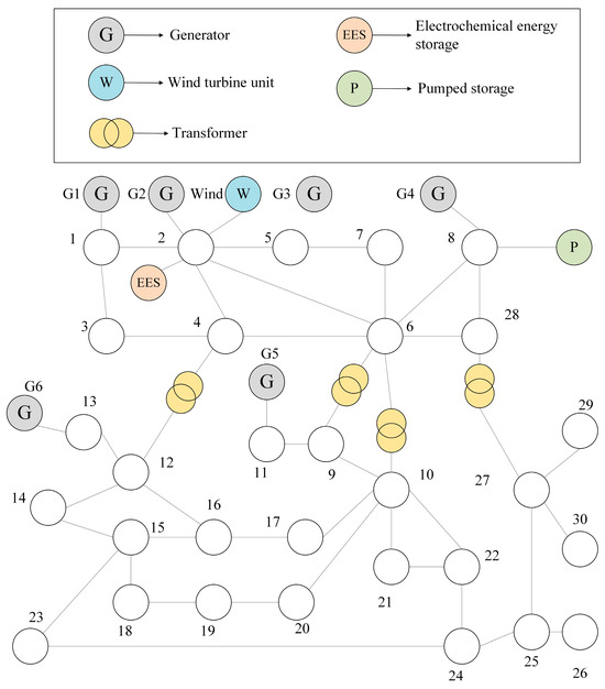
Figure 3.
Regional grid diagram.
Table 2.
Compensation cost factor of IDR.
The load and wind power predictions are generated based on the measured data plus white noise (the prediction error follows a normal distribution). The time scale of the measured curve is expanded from 1 h to 15 min, meaning that the same 4 data points are taken within each hour, totaling 96 data points. The prediction errors for the load’s day-ahead, intra-day, and real-time are 3%, 1%, and 0.5%, respectively. The prediction errors for the wind power’s day-ahead, intra-day, and real-time are 5%, 3%, and 1%, respectively. The measured and forecast curves for the load are shown in Figure 4.
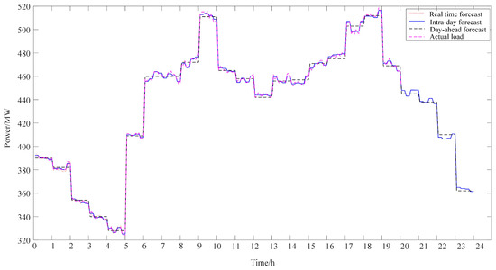
Figure 4.
The measured and forecast curves for the load.
6.2. Scheduling Result Analysis
Figure 5 shows the scheduling plans for the two scenarios of positive peak shaving and negative peak shaving of wind power. Each curve represents the total output of the previous curve plus the output of the corresponding unit (or DR resource). Figure 6 shows the DR resource scheduling plans for the two scenarios. Figure 7 shows the scheduling plans for pumped storage power stations and electrochemical power stations in the two scenarios.


Figure 5.
System scheduling plan.
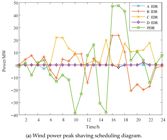
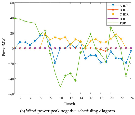
Figure 6.
DR resource scheduling plan.
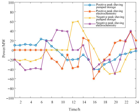
Figure 7.
Energy storage power station scheduling plan.
Analyzing the scheduling plans of the two scenarios separately, the following conclusions can be drawn:
- (1)
- When wind power is for positive peak shaving, the trend of the wind power output curve is basically consistent with the load curve. The high-output period of wind power is midday (10:00–14:00) and afternoon (16:00–19:00). During this period, the non-demand response load in the system is high, and the amount of IDR resources called is less than that in the negative peak shaving scenario during the same period.
- (2)
- When wind power is for negative peak shaving, the trend of the wind power output curve does not match the load curve. The high-output period of wind power is early morning (2:00–6:00) and evening (16:00–21:00). During this period, the non-demand response load in the system is low. Through the positive calling of IDR resources and the charging of the energy storage station, the wind power consumption level in this period is improved.
- (3)
- As can be seen from the calling plans of each part in Figure 6, the main task of power adjustment is still undertaken by the conventional units, which fulfill the tasks of peak shaving and frequency scheduling. IDR types, due to their relatively smaller adjustment volume limit, can only respond to the more drastic power adjustment quantities.
- (4)
- From the calling situation of various DR resources in Figure 7, it can be generally observed that during the day, IDR resources are mainly used for peak shaving and stabilizing wind power fluctuations, while at night, IDR resources are mainly used for valley filling.
- (5)
- From Figure 6, it can be seen that when wind power is adjusting the peak, the storage adjustment volume is smaller than that in the scenario where wind power is adjusting the peak in the opposite direction. In the face of sudden changes in wind power and load, pumped storage energy cannot achieve rapid response and scheduling, while electrochemical energy storage can complete rapid response and scheduling. The existence of these two types of energy storage stations can better provide peak shaving and valley filling capabilities. Combined with Figure 7, the wind power curtailment situation has basically been eliminated.
6.3. Comparison and Analysis of Scheduling Mode Strategies
In order to demonstrate the effect of integrating two types of energy storage power stations on improving the wind power consumption rate, reducing wind power curtailment, and lowering system costs, this paper also discusses the cases in two scenarios of positive and negative peak scheduling of wind power.
Scheduling scheme 1: Without the participation of energy storage power stations and without considering multi-time-scale scheduling, all scheduling plans are day-ahead scheduling plans.
Scheduling scheme 2: With the participation of pumped storage energy storage power stations, without considering multi-time-scale scheduling, all scheduling plans are day-ahead scheduling plans.
Scheduling scheme 3: The scheduling strategy of this paper. That is, multi-time-scale scheduling with the participation of the two types of energy storage power stations.
Table 3 presents the comparison results of three different scheduling schemes.
Table 3.
Comparison of different scheduling schemes in the new case.
- (1)
- Scheduling scheme 1 without the participation of an energy storage station, especially in the scenario of wind power counter-peak shaving, during the high wind power generation periods (2:00–6:00, 16:00–21:00), a small amount of demand response load cannot meet the large-scale consumption of wind power, resulting in a serious wind power abandonment phenomenon, with an abandonment rate of 23.34%.
- (2)
- Scheduling scheme 2 with a single pumped storage hydropower station participating, since the pumped storage power station does not have the characteristic of rapid scheduling, it cannot respond in time in the wind power counter-peak shaving scenario. Therefore, in the counter-peak shaving scenario and the positive peak shaving scenario, the abandonment rate of this scheduling strategy mode for the two scenarios is basically the same.
- (3)
- Scheduling scheme 3 with the participation of two energy storage stations, the rapid scheduling characteristic of the electrochemical energy storage station and the large-capacity high-power operation of the pumped storage power station form a complementarity. Combined with the small-scale scheduling of the demand response resources, it is possible to achieve a significant reduction in the wind power abandonment rate and a significant reduction in the system operation cost in both positive and negative peak shaving scenarios.
In conclusion, compared with the study on the improvement of the renewable energy consumption capacity of the “source–grid–load–storage” system by a single pumped storage energy storage station, the multi-time-scale scheduling strategy considering the characteristics of two energy storage stations proposed in this paper can better eliminate the adverse effects brought by the uncertainty of renewable energy prediction and better enhance the renewable energy consumption capacity.
To better verify the optimization of the renewable energy consumption capacity and system operation cost of the proposed method in different power grid environments for the regional power grid, based on the grid structure of the previous case, the placement positions and capacity configurations of conventional units, the capacity configuration and output characteristics of energy storage stations were changed, and this was used as a new example to verify the wide applicability of the proposed method. The topology diagram is shown in Figure 8.
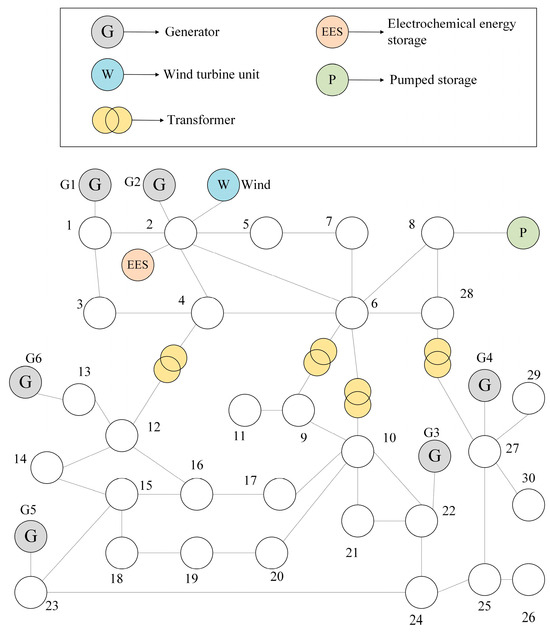
Figure 8.
New regional grid diagram.
The conventional thermal power units are located at nodes 1, 2, 22, 27, 23, and 13, and the parameters of the thermal power units are shown in Table 4. Node 2 is connected to a 400 MW wind farm and is in the counter-peak shaving scenario. At the same time, node 2 is connected to a 10 MW/40 MW·h electrochemical energy storage station, and node 8 is connected to a 40 MW/100 MW·h pumped storage power station. The DR resource configuration and the wind power load prediction results are the same as before, and will not be repeated here.
Table 4.
Parameters of conventional unit in the new case.
A comparison of scheduling schemes was conducted for the wind power positive peak shaving scenario with a higher wind power abandonment rate. The scheme settings were the same as before, and the results are shown in Table 5.
Table 5.
Comparison of different scheduling schemes.
Compared with the regional power grid in the new case, after changing the power grid topology, as can be seen from the results of the scheduling scheme 1, the wind power consumption capacity of the regional power grid without the participation of energy storage stations remains basically the same after the power source distribution position is changed. However, the system operation cost has changed to a certain extent due to the different distribution of generator output. According to the results of the scheduling schemes 2 and 3, the reduction in the capacity configuration of the energy storage station makes it impossible for the energy storage station to absorb the wind power during peak periods, resulting in an increase in the grid’s wind power rejection rate and cost compared to before. However, the new case verification shows that the method proposed in this paper can improve the renewable energy consumption capacity of the regional power grid and reduce the operation cost of the regional power grid in different power grid environments.
7. Conclusions
This paper proposes a “source–storage–load” scheduling plan that comprehensively considers the time characteristics of pumped storage and electrochemical energy storage power stations, as well as the multi-time-scale characteristics of DR resources. The output characteristics of the two types of energy storage power stations are analyzed, and they interact with DR resources based on their multi-time-scale characteristics, achieving the formulation of the day-ahead scheduling plan. Through the intra-day rolling and real-time correction, the uncertainty of renewable energy prediction and load prediction is suppressed to a certain extent. The results of the example show:
- (1)
- The participation of the two types of energy storage power stations in the scheduling plan can improve the consumption of wind power, reduce the wind power penalty cost, and thereby reduce the system operation cost. A formal Pareto-front analysis, mapping total cost against different levels of reliability (e.g., by varying the penalty costs or chance-constraint confidence levels), is identified as a key focus for future work to provide planners with a comprehensive decision-making tool.
- (2)
- The electrochemical energy storage power station has a rapid scheduling capability, which can effectively complement the scheduling capacity of the pumped storage energy storage power station, providing better storage space for wind power and thermal power during peak periods. It realizes the peak scheduling effect in different time periods.
- (3)
- The multi-time-scale can better utilize the rapid scheduling capabilities of electrochemical energy storage power stations and DR resources. This enables the system to improve the accuracy of the forecast data.
- (4)
- The proposed scheduling method in this paper can be widely applied in regional power grids with limited renewable energy output, improving the wind power consumption capacity.
By comparing the research conclusions of the scheduling strategies in [20,21] that only consider demand response, this paper conducts a time-characteristic-based study on energy storage power stations, combining the large-power storage effect of pumped storage and the rapid scheduling characteristics of electrochemical energy storage, more effectively alleviating the large-scale wind power rejection phenomenon caused by the inverse distribution of wind power output and load demand, and more effectively improving the wind power consumption capacity. It has a better reference effect for the consumption of new energy in the “source–grid–load–storage” system.
8. Future Work
- (1)
- The scheme in this paper only considers lithium batteries as the composition of electrochemical energy storage power stations. Different battery types and energy storage technologies have different output characteristics [22]. The future power system will connect various large-scale energy storage systems, and the modeling methods for various energy storage technologies are different. Further research in the following studies can be conducted on various energy storage technologies and various electrochemical energy storage technologies. The performance of the proposed scheduling strategy under extreme conditions, such as generator outages or significant market price fluctuations, represents a critical and valuable direction for future research.
- (2)
- One limitation of the current work is that the scenario-based stochastic programming approach does not explicitly capture the temporal dependencies of uncertainties (e.g., the Markovian property of wind power forecasting errors) [23,24]. Future research will explore more advanced modeling frameworks, such as multi-stage stochastic programming or stochastic dynamic programming, to incorporate these temporal correlations. This would enhance the decision-making process by making it more adaptive to the evolution of uncertainties over time. Furthermore, we have explicitly acknowledged in the manuscript’s outlook section that investigating the actual, observed levels of IDR participation across different consumer categories to establish a realistic baseline constitutes a key objective for our future research.
- (3)
- The confidence levels (α and β) in the chance constraints were set to a fixed value of 0.95 in this work. A sensitivity analysis to investigate the trade-offs between operational cost, reliability, and different confidence levels represents an important direction for future research.
- (4)
- The model, especially for IDR Type D (real-time), assumes an idealized instantaneous response without significant latency or ancillary costs. In practice, factors such as communication delays, the need for advanced metering infrastructure, and incentive costs for participants would impact the performance and economics of real-time response programs. These factors represent an important area for future model refinement to enhance practical applicability.
- (5)
- While the results demonstrate the efficacy of the proposed strategy for the chosen system configuration, a systematic exploration of the impact of different storage capacities on system performance and cost presents a significant opportunity for subsequent research.
- (6)
- A recognized limitation of this study is its focus on lithium-ion battery technology. While this provides a critical baseline analysis, the generalizability of the results to other emerging storage technologies, such as flow batteries or sodium-ion batteries, which may offer different characteristics in terms of cycle life, cost, and scalability, remains an important area for future investigation. This work establishes a foundational framework that can be adapted for such comparative techno-economic analyses.
- (7)
- Furthermore, while the proposed model demonstrated computational tractability for the case study system, its scalability to very large-scale networks with hundreds of nodes and a high penetration of distributed energy resources warrants further investigation. Future work will explore the use of decomposition techniques (e.g., Benders’ decomposition, alternating direction method of multipliers) or heuristic approaches to enhance computational efficiency for large-scale implementations.
Author Contributions
Conceptualization, B.Y.; Methodology, S.W.; Supervision, P.Z.; Writing—original draft, Y.G.; Writing—review & editing, B.M.; Validation, Y.L. and Q.H. All authors have read and agreed to the published version of the manuscript.
Funding
This research was funded by the Shaanxi Provincial Key R&D Program Project—Research on Carbon Reduction Effects and Key Technologies for Engineering Ecological Environmental Protection in Pumped Storage Power Stations (2024SF-ZDCYL-05-10). We also greatly appreciate the helpful suggestions and comments of editors and reviewers.
Data Availability Statement
The original contributions presented in this study are included in the article. Further inquiries can be directed to the corresponding author.
Conflicts of Interest
Authors Bo Yi, Sheliang Wang and Pin Zhang were employed by the company Power China Northwest Engineering Co., Ltd. Author Yan Liang was employed by the company Xi’an Power Supply Company, State Grid Shaanxi Electric Power Co., Ltd. The remaining authors declare that the research was conducted in the absence of any commercial or financial relationships that could be construed as a potential conflict of interest.
References
- Fitriani, A.; Amirullah, A.; Bhumkittipich, K. Power Quality Enhancement Using Single Phase Shunt Active Filter Based ANFIS Supplied by Photovoltaic. Vokasi Unesa Bull. Eng. Technol. Appl. Sci. 2025, 2, 558–580. [Google Scholar] [CrossRef]
- Kid, A.M.; Ahmed, M.Z.; Alkali, A.H.; Usman, J.; Hashim, A.H.A. Real-Time Energy Demand Forecasting and Adaptive Demand Response Optimization for IoT-Enabled Smart Grids. Vokasi Unesa Bull. Eng. Technol. Appl. Sci. 2025, 2, 366–375. [Google Scholar] [CrossRef]
- Gao, C.; Li, Q.; Li, H.; Zhai, H.; Zhang, L. Methodology and operation mechanism of demand response resources integration based on load aggregator. Autom. Electr. Power Syst. 2013, 37, 78–86. [Google Scholar] [CrossRef]
- Zhang, Y.; Ma, C.; Lian, J.; Pang, X.; Qiao, Y.; Chaima, E. Optimal photovoltaic capacity of large-scale hydro-photovoltaic complementary systems considering electricity delivery demand and reservoir characteristics. Energy Convers. Manag. 2019, 195, 597–608. [Google Scholar] [CrossRef]
- Prasad, A.A.; Taylor, R.A.; Kay, M. Assessment of solar and wind resource synergy in Australia. Appl. Energy 2017, 190, 354–367. [Google Scholar] [CrossRef]
- Zhang, F.; Zhang, T.; Wang, R.; Zheng, X.; Zhang, Y. System energy management research of energy local area network based on cooperative optimization of multiple generation-load-storage. Power Syst. Technol. 2017, 41, 3942–3950. [Google Scholar] [CrossRef]
- Jiang, Q.; Huang, K.; Zhao, J.; Sun, X. Study of “power-network load storage” coordinated optimization model for active distribution network based on genetic algorithm. Power Energy 2020, 41, 1–5, 19. [Google Scholar]
- Zhang, X.; Deng, L.; Li, J.; Wang, K.; Chen, W.; Li, J. General Coordinated Reactive Power Optimization of Active Distribution Network on the Basis of Scenario Time Domain Probability. Electr. Power Constr. 2018, 39, 2–8. [Google Scholar] [CrossRef]
- Xu, J.; X, J.; Xu, H. Research on source-gridload-storage optimization management based on energy router. Power Demand Side Manag. 2018, 20, 16–17, 21. [Google Scholar] [CrossRef]
- Li, Z.; Lei, X.; Qiu, S.; Liu, Z.; Zhang, L. Coordinated planning of active distribution network considering “source-grid-load” benefits. Power Syst. Technol. 2017, 41, 378–387. [Google Scholar] [CrossRef]
- Li, Y.; Han, X.; Li, T.; Zhou, X.; Xiao, C. A multifaceted low-carbon trading approach for integrated energy systems accounting for dynamicelectricity-carbon demand response. Autom. Electr. Power Syst. 2024, 48, 24–35. [Google Scholar] [CrossRef]
- Li, Q.; Xiao, X.; Pu, Y.; Luo, S.; Liu, H.; Chen, W. Hierarchical optimal scheduling method for regional integrated energy systems considering electricity-hydrogen shared energy. Appl. Energy 2023, 349, 121670. [Google Scholar] [CrossRef]
- Zhou, L.; Yu, H.; Li, P. Stochastic robust operation optimization for park-level integrated energy system in multi-stakeholder market. Autom. Electr. Power Syst. 2023, 47, 100–109. [Google Scholar] [CrossRef]
- Peng, Q.; Wang, X.; Kuang, Y.; Wang, Y.; Zhao, H.; Wang, Z.; Lyu, J. Hybrid energy sharing mechanism for integrated energy systems based on the Stackelberg game. CSEE J. Power Energy Syst. 2021, 7, 911–921. [Google Scholar] [CrossRef]
- Bao, Y.; Wang, B.; Li, Y.; Yang, S. Rolling dispatch model considering wind penetration and multi-scale demand response resources. Proc. CSEE 2016, 36, 4589–4600. [Google Scholar] [CrossRef]
- Cui, Y.; Zhang, J.; Zhong, W.; Wang, Z.; Zhao, Y. Scheduling strategy of wind penetration multi-source system considering multi-time scale source-load coordination. Power Syst. Technol 2021, 45, 1828–1837. [Google Scholar] [CrossRef]
- He, H.; Zhang, N.; Du, E.; Ge, Y.; Kang, C. Review on modeling method for operation efficiency and lifespan decay of large-scale electrochemical energy storage on power grid side. Autom. Electr. Power Syst. 2020, 44, 193–207. [Google Scholar] [CrossRef]
- Ju, L.; Yu, C.; Tan, Z. A two-stage scheduling optimization model and corresponding solving algorithm for power grid containing wind farm and energy storage system considering demand response. Power Syst. Technol. 2015, 39, 1287–1293. [Google Scholar] [CrossRef]
- Han, K.H.; Kim, J.H. Genetic quantum algorithm and its application to combinatorial optimization problem. In Proceedings of the 2000 Congress on Evolutionary Computation, La Jolla, CA, USA, 16–19 July 2000; CEC00 (Cat. No. 00TH8512). IEEE: Piscataway, NJ, USA, 2000; Volume 2, pp. 1354–1360. [Google Scholar] [CrossRef]
- Peng, C.; Yu, Y.; Sun, H. Planning of combined PV-ESS system for distribution network based on source-network-load collaborative optimization. Power Syst. Technol. 2019, 43, 3944–3951. [Google Scholar] [CrossRef]
- Han, Z.; Zhang, B.; Cui, K. Research on Joint Scheduling Strategy of Wind-Solar-Thermal Power Storage System Considering New Energy Accommodation Capacityand Power Generation Cost. Electr. Eng. 2020, 8, 21–25. [Google Scholar] [CrossRef]
- Zhang, Q.; Wang, X.; Wang, J.; Feng, C.; Liu, L. Survey of demand response research in deregulated electricity markets. Autom. Electr. Power Syst. 2008, 32, 97–106. [Google Scholar]
- Yang, Z.; Liu, P.; Cheng, L.; Liu, D.; Ming, B.; Li, H.; Xia, Q. Sizing utility-scale photovoltaic power generation for integration into a hydropower plant considering the effects of climate change: A case study in the Longyangxia of China. Energy 2021, 236, 121519. [Google Scholar] [CrossRef]
- Zhang, N.; Hu, Z.; Zhou, Y.; Xiao, X.; Wang, Y.; Cong, X. A novel fuzzy bi-objective unit commitment model considering demand side low-carbon resources. Autom. Electr. Power Syst. 2014, 38, 25–30. [Google Scholar] [CrossRef]


Disclaimer/Publisher’s Note: The statements, opinions and data contained in all publications are solely those of the individual author(s) and contributor(s) and not of MDPI and/or the editor(s). MDPI and/or the editor(s) disclaim responsibility for any injury to people or property resulting from any ideas, methods, instructions or products referred to in the content. |
© 2025 by the authors. Licensee MDPI, Basel, Switzerland. This article is an open access article distributed under the terms and conditions of the Creative Commons Attribution (CC BY) license (https://creativecommons.org/licenses/by/4.0/).