Multi-Scale Graph Learning with Seasonal and Trend Awareness Electricity Load Forecasting

Abstract

Accurate electricity load forecasting underpins smart-grid operation and broader economic planning. Yet multivariate load series are driven by weather, economic activity, and seasonal effects whose intertwined, scale-dependent dynamics make forecasting challenging. While graph neural networks (GNNs) capture spatio-temporal dependencies, they often underrepresent multi-scale structure. MTSGNN (multi-scale trend–seasonal GNN) is introduced to bridge this gap. MTSGNN couples a multi-scale trend–seasonal GNN module with a Hawkes-enhanced temporal decoder. The former decomposes load signals into multiple temporal scales and models cross-variable interactions at each scale, while the latter embeds a Hawkes process to capture decaying and self-/mutually exciting temporal influences. To effectively combine long-term trends with periodic variations, a Trend–Seasonal Spatio-Temporal Fusion mechanism is proposed, which jointly learns and integrates trend and seasonal representations across both space and time. MTSGNN is designed for multi-step load forecasting with a historical window of 120 time steps and a prediction horizon of 120 future steps. Evaluations on five real-world datasets demonstrate that MTSGNN consistently surpasses existing approaches for multi-step power load prediction, establishing a new benchmark in forecasting accuracy.

1. Introduction

A reliable electricity supply is crucial for driving economic growth [1,2,3]. For power utilities, electricity load forecasting plays a vital role in optimizing the generation and distribution of electricity, predicting future demand based on historical consumption data [4,5]. Accurate forecasting ensures grid stability and reduces costs. The adoption of smart grids increases sensor deployment, complicating spatio-temporal dependencies and making forecasting more challenging [6].

Electricity load forecasting spans short-term (minutes–week), medium-term (month–year), and long-term (years) [7,8,9]. Short-term multi-step forecasting has attracted increasing attention due to its practical value in identifying supply–demand fluctuations and assisting real-time electricity dispatch.

Traditionally, forecasting relies on temporal dependencies inferred from past load dynamics. Statistical methods (e.g., ARIMA [10]) capture linear trends; machine learning (e.g., SVM [11], XGBoost [12], LightGBM [13]) models nonlinearities but struggles with volatility; deep models (LSTM [14], GRU [15], Transformers [16]) improve temporal modeling but often neglect spatial dependencies.

Graph neural networks (GNNs) [17] have been increasingly applied in load forecasting to capture pairwise sensor dependencies [18]. Sensors are represented as nodes, and edges encode dependencies. Combining GNNs with temporal modules allows capturing spatio-temporal patterns effectively [19,20].

However, two challenges remain in electricity load forecasting. First, electricity time series inherently exhibit multi-scale characteristics, where fine-grained data capture short-term fluctuations while coarse-grained data reveal long-term trends and periodicity, as illustrated in Figure 1. Correspondingly, sensor relationships vary across scales: fine-grained scales reflect fluctuation-related correlations, whereas coarse-grained scales capture trend-related correlations. On the one hand, single-scale decomposition methods like Autoformer decouple time series into trend and seasonal components but only at a fixed scale, thereby failing to capture complementary cross-scale interactions between trend and seasonal features [21]. On the other hand, existing multi-scale methods primarily focus on modeling temporal dependencies at different resolutions but largely ignore inter-variable relationships, e.g., trend and seasonal correlations across sensors [22,23]. Thus, existing methods rarely account for these scale-dependent dependencies, limiting their ability to jointly model short-term variations and long-term patterns. Second, historical fluctuations exhibit a temporal decay effect, where recent variations exert stronger influence on future demand than older observations. Many existing methods assume uniform influence of past observations, which fails to reflect this natural decline [24,25]. Ignoring temporal decay can lead to biased predictions, as models may overemphasize outdated information while underweighting more relevant recent patterns. Therefore, accurately modeling the decay effect is crucial for capturing temporal dynamics and improving forecast reliability.

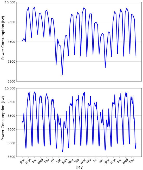
Figure 1. The lower section displays raw electricity load data sampled at 30 min intervals, while the upper section shows data at 6 h intervals.

To address these challenges, an end-to-end multi-scale trend–seasonal graph neural network (MTSGNN) is proposed for electricity load forecasting. The framework first generates multi-scale time series via down-sampling. A Hawkes-based temporal module captures the decline effect at each scale. Multi-scale trend and seasonal graphs model diverse sensor relationships, and spatio-temporal features are aggregated separately. Finally, a fusion module integrates these components to improve accuracy.

The main contributions of this work are summarized as follows:

• A multi-scale graph neural network (GNN) module is proposed to capture trend and seasonal dependencies across different temporal scales, addressing the limitations of existing approaches in modeling cross-scale relationships.
• A Hawkes attention mechanism is introduced to efficiently aggregate sequential features, enabling the model to capture the dynamic and time-varying characteristics of electricity demand.
• A trend–seasonal spatio-temporal fusion method is developed, which integrates trend and seasonal spatio-temporal features through an attention-driven strategy to further enhance prediction accuracy.
• Experimental results on multiple datasets indicate that the proposed model achieves superior predictive performance compared with both non-graph-based and graph-based electricity load forecasting methods.

The remainder of this paper is organized as follows. Section 2 reviews the related literature. Section 3 presents the overall framework and describes the details of the proposed MTSGNN. Section 4 outlines the experimental setup, including datasets, evaluation metrics, baseline models, and results, followed by an in-depth analysis. Finally, Section 5 provides concluding remarks.

2. Related Works

2.1. Non-Graph-Based Models

Statistical approaches, such as Autoregressive Integrated Moving Average (ARIMA) [26], handle seasonal data well but struggle with nonlinear fluctuations. For example, Ediger et al. analyzed electricity forecasting in Turkey, highlighting the reliability of regression and ARIMA models [27]. Holt-Winters and its extensions [28,29] effectively capture seasonal patterns through exponential smoothing, but they treat variables independently and ignore inter-variable dependencies. However, compared to deep learning approaches, these methods often fail to capture complex nonlinear patterns, leading to suboptimal performance [30].

With advances in computing, machine learning methods like SVM [11], XGBoost [12], and LightGBM [13] have been widely applied to electricity load forecasting [31]. These methods improve computational efficiency and can model nonlinearities, but their predictive accuracy is often limited by simpler network structures.

Deep learning architectures have further transformed load forecasting, enabling hierarchical feature learning to capture complex temporal dynamics [32]. Innovations include hybrid architectures combining feature selection with deep networks [33], RNN variants (LSTM/GRU) and hybrid sequential models [34], as well as multimodal and multivariate approaches integrating CNN, attention, and XGBoost frameworks [25,35]. Despite these advances, traditional methods still primarily focus on temporal patterns and often neglect spatial dependencies among sensors.

2.2. Graph-Based Models

Graph-based learning has advanced the modeling of spatial dependencies in sensor networks. GNN architectures have been proposed to handle complex interactions in electricity load forecasting. Examples include attentive transfer frameworks [36], dual-path graph networks [37], and hybrid graph constructions combining static topology with dynamic embeddings [20]. Unified spatio-temporal GCNs [38] and graph-nested transformers [23] further optimize spatial adjacency and temporal continuity while embedding hierarchical dependencies.

Nevertheless, existing graph-based methods often overlook sensor relationships across multiple temporal scales and fail to account for the declining influence of historical fluctuations on future load.

3. Methodology

3.1. Overall Framework

Figure 2 illustrates the framework of the proposed MTS-GNN. It first employs the Multi-Scale Sampling module (MSM) to generate time series across different time scales. Then, the Multi-Scale Time Decomposition (MTD) module separates the multi-scale series into trend and seasonal components, which are processed by a Hawkes-based temporal module to capture temporal dependencies. Next, the Multi-Scale Spatial module models the spatial dependencies between different sensors at different scales using Graph Convolutional Networks (GCNs). Then, the scale-wise trend and seasonal aggregation module is introduced to obtain multi-scale trend features and seasonal spatio-temporal representations, respectively. Finally, the fused trend and seasonal spatio-temporal representations are integrated and fed into the prediction module for load forecasting.

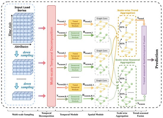
Figure 2. The framework of MTSGNN. The pipeline consists of the following steps: (1) Generating multi-scale time series (i.e., Multi-scale Sampling). (2) Decomposing multi-scale time series into trend and seasonal components (i.e., Temporal Decomposition). (3) Capturing temporal dependencies (i.e., Temporal Module). (4) Capturing spatio-temporal dependencies (i.e., Spatial Module). (5) Aggregating multi-scale trend and seasonal spatio-temporal representations, separately (i.e., Scale-wise Aggregation). (6) Fusing trends and seasonal representations for prediction (i.e., Trend–seasonal Fusion).

3.2. Multi-Scale Sampling Module

As illustrated in Figure 2, a multi-scale pooling strategy is employed to capture temporal dependencies across different time scales. The MSM module is composed of multiple down-sampling layers that transform the raw time series into feature representations ranging from fine- to coarse-grained levels. The fine-grained representations preserve local fluctuations, whereas the coarse-grained representations reflect broader temporal trends.

MSM hierarchically generates coarser-scale features from previous outputs. Given the input series $\mathbf{X}\in {\mathbb{R}}^{L\times D}$, MSM generates $K-1$ coarser scales. The feature representation at the k-th scale is denoted as ${\mathbf{X}}_k\in {\mathbb{R}}^{⌊{\displaystyle \frac{L}{2^k}}⌋\times D}$, where $⌊{\displaystyle \frac{L}{2^k}}⌋$ is the sequence length at the k-th scale and $\lfloor ·\rfloor$ denotes the floor operator. Formally,

$${\mathbf{X}}_k=Pooling\left({\mathbf{X}}_{k-1}\right),k=1,2,...,K-1,$$

(1)

where $Pooling(·)$ indicates average pooling performed along the temporal dimension. The multi-scale series ${\left\{{\mathbf{X}}_k\right\}}_{k=0}^{K-1}$, with ${\mathbf{X}}_0=\mathbf{X}$, is then fed into the subsequent module.

3.3. Multi-Scale Temporal Decomposition

Electricity load series often exhibit complex variations even at coarse temporal scales. In addition, the seasonal and trend components display distinct behaviors, corresponding to stationary and non-stationary dynamics [39]. Following the decomposition strategy in [21], the series at each scale is separated into a seasonal component ${\mathcal{X}}_{season}={\left\{{\mathbf{X}}_{season,k}\right\}}_{k=0}^{K-1}$ and a trend component ${\mathcal{X}}_{trend}={\left\{{\mathbf{X}}_{trend,k}\right\}}_{k=0}^{K-1}$. For the k-th scale ($k\in [0:K-1]$), the decomposition is formulated as follows:

$$\begin{array}{cc}\hfill {\mathbf{X}}_{trend,k}& =AvgPool{\left(Padding\left({\mathbf{X}}_k\right)\right)}_{kernel},\hfill \\ \hfill {\mathbf{X}}_{season,k}& ={\mathbf{X}}_k-{\mathbf{X}}_{trend,k},\hfill \end{array}$$

(2)

where ${\mathbf{X}}_{season,k}$ and ${\mathbf{X}}_{trend,k}$ share the same dimension as ${\mathbf{X}}_k$. Here, $AvgPool(·)$ indicates that the average pooling is performed only along the temporal dimension, while $Padding(·)$ ensures the series length remains constant. The detailed implementation of this decomposition process is shown in Algorithm 1.

Algorithm 1: Multi-scale Temporal Decomposition (PyTorch-like)

3.4. Multi-Scale Temporal Module

The multi-scale temporal module contains two sub-modules: trend and seasonal temporal modules, sharing the same framework but with different parameters.

Recent fluctuations have a stronger impact on electricity demand than older events. To capture this effect, temporal features of the trend and seasonal components are aggregated separately at each scale.

For the trend module, each sensor’s time series is first processed channel-wise using CNNs to extract informative patterns:

$${\overline{\mathbf{X}}}_{trend,k}^n=ReLU(\mathbf{W}\otimes {\mathbf{X}}_{trend,k}^n+\mathbf{b}),$$

(3)

where ${\overline{\mathbf{X}}}_{trend,k}^n\in {\mathbb{R}}^{{\displaystyle \frac{L}{2^k}}\times C}$, and ⊗ denotes convolution.

An LSTM then captures temporal dependencies:

$${\overline{\mathbf{H}}}_{trend,k}^n=LSTM\left({\overline{\mathbf{X}}}_{trend,k}^n\right)\in {\mathbb{R}}^{{\displaystyle \frac{L}{2^k}}\times D}.$$

(4)

Subsequently, previous studies on the Hawkes process have demonstrated that prior event stream can influence and drive subsequent fluctuations in continuous time [40]. It offers a flexible mathematical framework for modeling self-exciting processes through statistical and probabilistic principles. To capture the decline effect, Hawkes attention is employed to implement time-aware attention, enabling effective aggregation of the sequential features generated by the LSTM. Specifically, the weight associated with the p-th time step is computed as follows:

$${\lambda }^p={\displaystyle \frac{1+ϵexp(-\gamma \Delta t_p)}{{\sum }_u(1+ϵexp(-\gamma \Delta t_u))}},{\mathbf{H}}_{trend,k}^n=\sum _p{\lambda }^p{\overline{\mathbf{H}}}_{trend,k}^{n,p},$$

(5)

$ϵ$ is the excitation coefficient and $\gamma$ is the decay rate. Here, $\Delta t_p^k=t-p$ denotes the index difference between the current step and the p-th historical step at the k-th temporal scale. The seasonal component ${\mathbf{H}}_{season,k}^n$ is processed similarly.

3.5. Multi-Scale Spatial Module

3.5.1. Multi-Scale Graph Construction

Most existing graph-based methods learn a single adjacency matrix to capture inter-series dependencies, which primarily reflects short-term fluctuations. However, time series exhibit multiple types of relationships, such as trend and seasonal patterns, which vary across temporal scales. For example, trend-related dependencies often become more pronounced at coarser scales, providing a clearer characterization of long-term patterns. To capture such diverse relationships, multi-scale adjacency matrices are constructed for both the trend and seasonal components.

At the k-th scale, the adjacency matrices are computed using cosine similarity between temporal representations:

$$\begin{array}{cc}\hfill {\mathbf{A}}_{trend,k}(i,j)& ={\displaystyle \frac{{\mathbf{H}}_{trend,k}^i·{\mathbf{H}}_{trend,k}^j}{\parallel {\mathbf{H}}_{trend,k}^i\parallel \parallel {\mathbf{H}}_{trend,k}^j\parallel }},\hfill \\ \hfill {\mathbf{A}}_{season,k}(i,j)& ={\displaystyle \frac{{\mathbf{H}}_{season,k}^i·{\mathbf{H}}_{season,k}^j}{\parallel {\mathbf{H}}_{season,k}^i\parallel \parallel {\mathbf{H}}_{season,k}^j\parallel }},\hfill \end{array}$$

(6)

where ${\mathbf{A}}_{trend,k},{\mathbf{A}}_{season,k}\in {\mathbb{R}}^{N\times N}$ represent trend and seasonal inter-series relationships at the k-th scale.

3.5.2. Multi-Scale Graph Aggregation

To capture spatial dependencies among sensors, GCNs are applied to aggregate information based on the constructed adjacency matrices. Let ${\mathbf{H}}_{trend,k}^i$ and ${\mathbf{H}}_{season,k}^i$ denote the temporal representations of the i-th series for trend and seasonal components at scale k. The aggregation is formulated as

$$\begin{array}{cc}\hfill {\overline{\mathbf{S}}}_{trend,k}& =GC{N}_t({\mathbf{A}}_{trend,k},{\mathbf{H}}_{trend,k};{\Theta }_1),\hfill \\ \hfill {\overline{\mathbf{S}}}_{season,k}& =GC{N}_s({\mathbf{A}}_{season,k},{\mathbf{H}}_{season,k};{\Theta }_2),\hfill \end{array}$$

(7)

where ${\overline{\mathbf{S}}}_{trend,k}, {\overline{\mathbf{S}}}_{season, k}\in {\mathbb{R}}^{N\times F}$ are the spatio-temporal representations at scale k, and $GC{N}_{\ast }$ with ${\Theta }_{\ast }$ denote the respective models and parameters.

3.6. Scale-Wise Trend and Seasonal Aggregation

Given that trend and seasonal patterns exhibit distinct behaviors across temporal scales, the multi-scale spatio-temporal representations for trend and seasonality are integrated separately.

3.6.1. Trend Aggregation

Coarser scales offer clearer macro-level trend information, whereas finer scales may introduce additional noise. To leverage the strengths of both, a bottom-up fusion strategy is employed, in which coarse-scale knowledge is propagated to finer scales in a residual manner:

$${\widehat{\mathbf{S}}}_{trend,k}={\overline{\mathbf{S}}}_{trend,k}+FF{N}_t\left({\widehat{\mathbf{S}}}_{trend,k-1}\right),k\in \{1,2,...,K-1\},$$

(8)

where ${\widehat{\mathbf{S}}}_{trend,K-1}$ (denoted as ${\mathbf{S}}_{trend}$) is the final integrated trend representation, $FF{N}_t(·)$ is a feed-forward network, and ${\widehat{\mathbf{S}}}_{trend,0}={\overline{\mathbf{S}}}_{trend,0}$.

3.6.2. Seasonal Aggregation

Seasonal patterns are formed by aggregating finer-scale fluctuations. A top-down fusion strategy is employed to incorporate detailed seasonal features from finer scales into coarser scales:

$${\widehat{\mathbf{S}}}_{season,k}={\overline{\mathbf{S}}}_{season,k}+FF{N}_s\left({\widehat{\mathbf{S}}}_{season,k+1}\right),k\in \{K-2,...,0\},$$

(9)

where ${\widehat{\mathbf{S}}}_{season,0}$ (denoted as ${\mathbf{S}}_{season}$) is the final seasonal representation, and ${\widehat{\mathbf{S}}}_{season,K-1}={\overline{\mathbf{S}}}_{season,K-1}$.

This combines seasonal details and trend knowledge into a unified representation.

3.7. Trend–Seasonal Spatio-Temporal Fusion

To combine ${\mathbf{S}}_{trend}$ and ${\mathbf{S}}_{season}$ into a unified representation, an attention-based fusion mechanism is employed to capture their interactions while preserving the distinct characteristics of each component.

First, a fused embedding $\mathbf{V}\in {\mathbb{R}}^{F^{\prime }}$ is computed via multiple vector–matrix–vector multiplications:

$$\mathbf{V}={\mathbf{S}}_{trend}{\mathcal{F}}^{[1:F^{\prime }]}{\mathbf{S}}_{season},$$

(10)

where $\mathcal{F}\in {\mathbb{R}}^{F^{\prime }\times NF\times NF}$ is a learnable tensor.

Next, attention scores are computed by mapping trend and seasonal representations into query and key spaces:

$$\mathbf{Q}={\mathbf{S}}_{trend}{W}_Q,\mathbf{K}={\mathbf{S}}_{season}{W}_K,$$

(11)

with $W_Q$ and $W_K$ as learnable parameters. Finally, a scaled dot-product attention fuses features:

$$\mathbf{O}=\mathrm{Attention}(\mathbf{Q},\mathbf{K},\mathbf{V})=\mathrm{Softmax}\left(\tau {\displaystyle \frac{\mathbf{Q}{\mathbf{K}}^T}{\sqrt{K_d}}}\right)\mathbf{V},$$

(12)

where $\mathbf{O}$ is the fused trend–seasonal spatio-temporal representation, $\tau$ is the attention temperature, and $K_d$ is the scaling factor.

The overall computational complexity of the proposed trend–seasonal fusion can be roughly decomposed as follows. The vector–matrix–vector multiplications dominate the computation with a cost of $\mathcal{O}\left(F^{\prime }N{F}^2\right)$, where $F^{\prime }$ is the number of output features. The projection of trend and seasonal components into query and key spaces contributes $\mathcal{O}\left(N{F}^2\right)$. Finally, the scaled dot-product attention incurs an additional $\mathcal{O}\left(NF\right)$ for the weighted aggregation. Therefore, the total complexity can be approximated as $\mathcal{O}(F^{\prime }N{F}^2+N{F}^2+N^{2}F)$.

3.8. Prediction and Optimization

Subsequently, a two-layer feed-forward neural network is applied to predict future electricity load, formulated as

$$\widehat{\mathbf{Y}}=FN{N}_o\left(\mathbf{O}\right),$$

(13)

where $\widehat{\mathbf{Y}}$ denotes the predicted electricity load. $\mathbf{O}$ represents the fused spatio-temporal features. The function $FN{N}_o(·)$ corresponds to the two-layer feed-forward neural network with learnable parameters, which maps these features to the final load predictions.

Finally, all parameters are learned by minimizing the mean squared error (MSE) [41].

$$\mathcal{L}=MSE(\widehat{\mathbf{Y}},\mathbf{Y}).$$

(14)

4. Experiment

4.1. Datasets

Electricity Transformer Temperature (ETT): The ETT dataset [23] comprises power load variables and oil temperature data, providing a valuable benchmark for evaluating the model’s capacity to capture variable interactions and ensure robust time series predictions. Essential for power system reliability, this dataset spans two years across two regions in China and includes four subsets—ETTh1, ETTh2, ETTm1, and ETTm2—collected at 1 h and 15 min intervals.

Australian electricity load (AEL): AEL dataset consists of data from the Australian electricity market, incorporating various factors such as electricity demand, generation, pricing, and weather conditions.

Electricity. The large-scale Electricity dataset [42] is also used for evaluation. This dataset contains 321-dimensional electricity consumption records from the U.S. electricity grid and spans 26,304 time steps with a 15 min sampling interval, forming a high-dimensional and large-scale multivariate time series. Its complexity and scale make it particularly suitable for assessing a model’s capability to capture intricate interdependencies among numerous variables, as well as its scalability and robustness.

All the datasets are divided into training, validation, and testing sets with a ratio of 7:1:2. Table 1 summarizes the details of each dataset.

Table 1. Dataset statistics including the Electricity dataset. Training/validation/test splits are approximately 70%/10%/20%. Length corresponds to the history window length used for forecasting, and Sampling Rate indicates the time interval between consecutive measurements.

Dataset	# Train	# Val	# Test	Length	# Variable	Sampling Rate
ETTh1	12,194	1742	3484	120	7	Hourly
ETTh2	12,194	1742	3484	120	7	Hourly
ETTm1	48,776	6968	13,936	120	7	15 min
ETTm2	48,776	6968	13,936	120	7	15 min
AEL	61,353	8765	17,530	120	6	30 min
Electricity	18,412	2630	5262	168	321	Hourly

4.2. Baseline Methods

An organized evaluation protocol is adopted to ensure a comprehensive assessment. The analysis stratifies forecasting approaches into two categories: (1) Conventional non-graph architectures, and (2) Graph-aware models. This division enables systematic comparison of spatial–temporal modeling capabilities. The baselines include classical machine learning and modern neural architectures:

4.2.1. Non-Graph-Based Methods

Several classical non-graph-based approaches are included for comparison. ARIMA [26] represents a traditional autoregressive model used for linear analysis of electrical time series. LSTM [24] and GRU [43] are implemented as two-layer recurrent neural network variants. CNN-BiLSTM-Attention [25] combines convolutional neural networks, bidirectional LSTMs, and an attention mechanism, further enhanced by XGBoost stacking to improve short-term load forecasting performance.

4.2.2. Graph-Based Methods

Several graph-based methods are also included for comparison. GAT [44] utilizes attention mechanisms to adaptively weight the contributions of neighboring nodes, thereby enhancing feature extraction and graph representation. MTGNN [45] automatically learns variable relationships and captures spatial–temporal dependencies via propagation and inception layers. STEGNN [20] models spatial dependencies with dynamic graphs and temporal periodicity using trainable embeddings. SmartFormer [23] integrates graph neural networks with transformer layers to capture inter-series dependencies and optimize electric load forecasting. PatchFormer [42] is a multi-scale, patch-based Transformer with adaptive pathways that captures both global and local temporal dependencies across varying time resolutions, improving modeling of diverse temporal dynamics.

4.3. Implementation Details

All experiments are conducted on a single NVIDIA GeForce RTX 3070Ti GPU using PyTorch 2.1. Each model is trained for 100 epochs with a batch size of 32, using the ADAM optimizer [46] with a learning rate of 5 × 10⁻³. To ensure reliable evaluation, every experiment is conducted independently five times, and the average performance is reported. A fixed random seed is used across all experiments to maintain reproducibility, and all models are executed under the same seed, with results averaged over the repeated runs.

4.4. Result Analysis

Table 2 presents a comparison between the proposed method and both non-graph-based and graph-based models. Five independent experiments are conducted, and t-tests with a significance level of $\alpha =0.01$ are applied. A p-value below $\alpha$ indicates a statistically significant difference in performance. Accordingly, smaller p-values reflect stronger evidence that the proposed method outperforms the baseline approaches.

Table 2. Performance comparison with baselines on six datasets (ETTh1, ETTh2, ETTm1, ETTm2, AEL, Electricity). Bold and Underline show the best and second best results, respectively. ‘Std’ represents the standard deviation.

	Methods	Metrics	ETTh1		ETTh2		ETTm1		ETTm2		AEL		Electricity
			Value	p-Value	Value	p-Value	Value	p-Value	Value	p-Value	Value	p-Value	Value	p-Value
Non-graph -based	ARIMA	MSE	1.043	$6.78\times {10}^{-13}$	0.906	$1.87\times {10}^{-11}$	0.961	$5.77\times {10}^{-12}$	0.808	$9.10\times {10}^{-12}$	0.726	$5.87\times {10}^{-10}$	0.912	$1.23\times {10}^{-11}$
		MAE	0.815	$2.65\times {10}^{-10}$	0.687	$4.74\times {10}^{-13}$	0.793	$8.41\times {10}^{-8}$	0.671	$1.87\times {10}^{-11}$	0.665	$6.46\times {10}^{-8}$	0.702	$4.56\times {10}^{-9}$
		MAPE	0.325	$3.42\times {10}^{-9}$	0.298	$2.98\times {10}^{-10}$	0.316	$5.72\times {10}^{-8}$	0.289	$1.34\times {10}^{-9}$	0.274	$3.88\times {10}^{-7}$	0.296	$3.41\times {10}^{-8}$
	Holt-Winters	MSE	0.985	$4.12\times {10}^{-12}$	0.812	$2.35\times {10}^{-11}$	0.901	$6.47\times {10}^{-12}$	0.790	$1.02\times {10}^{-11}$	0.701	$6.13\times {10}^{-10}$	0.845	$2.14\times {10}^{-11}$
		MAE	0.802	$3.58\times {10}^{-10}$	0.676	$5.24\times {10}^{-13}$	0.781	$7.98\times {10}^{-8}$	0.663	$1.65\times {10}^{-11}$	0.652	$7.14\times {10}^{-8}$	0.689	$4.21\times {10}^{-9}$
		MAPE	0.317	$3.56\times {10}^{-9}$	0.285	$3.01\times {10}^{-10}$	0.308	$5.14\times {10}^{-8}$	0.276	$1.18\times {10}^{-9}$	0.263	$3.55\times {10}^{-7}$	0.287	$3.02\times {10}^{-8}$
	LSTM	MSE	0.928	$2.09\times {10}^{-11}$	0.595	$4.97\times {10}^{-10}$	0.778	$2.35\times {10}^{-11}$	0.739	$9.85\times {10}^{-12}$	0.613	$5.59\times {10}^{-9}$	0.682	$7.21\times {10}^{-10}$
		MAE	0.791	$5.31\times {10}^{-11}$	0.571	$5.54\times {10}^{-9}$	0.595	$1.48\times {10}^{-10}$	0.602	$8.82\times {10}^{-11}$	0.617	$8.56\times {10}^{-10}$	0.645	$2.34\times {10}^{-9}$
		MAPE	0.284	$4.01\times {10}^{-9}$	0.236	$2.19\times {10}^{-9}$	0.228	$3.43\times {10}^{-8}$	0.241	$2.89\times {10}^{-8}$	0.235	$6.12\times {10}^{-8}$	0.229	$2.01\times {10}^{-8}$
	GRU	MSE	0.958	$6.67\times {10}^{-11}$	0.608	$3.00\times {10}^{-7}$	0.786	$3.98\times {10}^{-9}$	0.776	$4.71\times {10}^{-10}$	0.635	$2.23\times {10}^{-7}$	0.695	$1.05\times {10}^{-9}$
		MAE	0.798	$8.78\times {10}^{-9}$	0.583	$1.57\times {10}^{-9}$	0.604	$5.86\times {10}^{-11}$	0.579	$5.33\times {10}^{-10}$	0.650	$4.58\times {10}^{-8}$	0.658	$6.12\times {10}^{-10}$
		MAPE	0.278	$3.67\times {10}^{-9}$	0.241	$2.64\times {10}^{-9}$	0.235	$4.87\times {10}^{-8}$	0.222	$2.68\times {10}^{-8}$	0.239	$5.44\times {10}^{-8}$	0.230	$2.06\times {10}^{-8}$
	CNN-BiLSTM -Attention	MSE	0.876	$3.71\times {10}^{-10}$	0.675	$1.42\times {10}^{-8}$	0.507	$4.61\times {10}^{-7}$	0.762	$7.92\times {10}^{-10}$	0.526	$7.85\times {10}^{-7}$	0.491	$1.45\times {10}^{-8}$
		MAE	0.759	$2.04\times {10}^{-7}$	0.585	$1.73\times {10}^{-9}$	0.505	$4.36\times {10}^{-9}$	0.576	$2.75\times {10}^{-7}$	0.537	$8.43\times {10}^{-6}$	0.490	$5.32\times {10}^{-7}$
		MAPE	0.254	$2.10\times {10}^{-8}$	0.217	$2.65\times {10}^{-9}$	0.196	$4.20\times {10}^{-8}$	0.208	$1.99\times {10}^{-8}$	0.183	$3.41\times {10}^{-7}$	0.179	$2.11\times {10}^{-7}$
Graph -based	GAT	MSE	0.629	$2.86\times {10}^{-7}$	0.598	$5.90\times {10}^{-7}$	0.569	$6.58\times {10}^{-8}$	0.651	$7.47\times {10}^{-6}$	0.602	$3.39\times {10}^{-9}$	0.442	$2.11\times {10}^{-7}$
		MAE	0.585	$7.40\times {10}^{-8}$	0.577	$3.15\times {10}^{-9}$	0.538	$2.56\times {10}^{-6}$	0.558	$1.48\times {10}^{-9}$	0.614	$1.38\times {10}^{-10}$	0.420	$1.25\times {10}^{-7}$
		MAPE	0.209	$2.65\times {10}^{-8}$	0.212	$2.61\times {10}^{-9}$	0.200	$2.15\times {10}^{-7}$	0.196	$1.72\times {10}^{-8}$	0.208	$3.92\times {10}^{-8}$	0.159	$1.19\times {10}^{-7}$
	MTGNN	MSE	0.561	$4.65\times {10}^{-9}$	0.537	$9.96\times {10}^{-5}$	0.474	$1.28\times {10}^{-6}$	0.599	$9.50\times {10}^{-6}$	0.421	$5.92\times {10}^{-6}$	0.387	$3.11\times {10}^{-6}$
		MAE	0.533	$1.18\times {10}^{-8}$	0.529	$4.22\times {10}^{-5}$	0.472	$6.25\times {10}^{-7}$	0.510	$8.19\times {10}^{-9}$	0.442	$3.24\times {10}^{-7}$	0.355	$2.18\times {10}^{-6}$
		MAPE	0.195	$1.64\times {10}^{-8}$	0.192	$3.47\times {10}^{-5}$	0.184	$5.12\times {10}^{-7}$	0.179	$7.15\times {10}^{-9}$	0.162	$2.88\times {10}^{-7}$	0.138	$1.91\times {10}^{-6}$
	STEGNN	MSE	0.446	$9.80\times {10}^{-6}$	0.536	$6.82\times {10}^{-5}$	0.510	$6.36\times {10}^{-3}$	0.327	$2.13\times {10}^{-6}$	0.396	$4.39\times {10}^{-5}$	0.301	$3.52\times {10}^{-5}$
		MAE	0.438	$4.09\times {10}^{-7}$	0.533	$3.75\times {10}^{-5}$	0.490	$1.03\times {10}^{-7}$	0.356	$2.05\times {10}^{-3}$	0.411	$9.92\times {10}^{-4}$	0.384	$1.21\times {10}^{-4}$
		MAPE	0.167	$3.89\times {10}^{-6}$	0.193	$3.52\times {10}^{-5}$	0.176	$5.49\times {10}^{-4}$	0.141	$1.38\times {10}^{-3}$	0.158	$8.63\times {10}^{-4}$	0.129	$1.09\times {10}^{-4}$
	SmartFormer	MSE	0.434	$3.73\times {10}^{-5}$	0.530	$1.84\times {10}^{-4}$	0.455	$3.58\times {10}^{-4}$	0.334	$2.99\times {10}^{-5}$	0.392	$8.42\times {10}^{-5}$	0.195	$6.12\times {10}^{-5}$
		MAE	0.430	$3.21\times {10}^{-3}$	0.528	$4.68\times {10}^{-4}$	0.484	$5.45\times {10}^{-3}$	0.370	$6.31\times {10}^{-4}$	0.403	$2.38\times {10}^{-4}$	0.280	$3.24\times {10}^{-4}$
		MAPE	0.159	$3.02\times {10}^{-4}$	0.190	$3.97\times {10}^{-4}$	0.172	$4.68\times {10}^{-3}$	0.147	$5.92\times {10}^{-4}$	0.154	$2.16\times {10}^{-4}$	0.101	$2.83\times {10}^{-4}$
	PathFormer	MSE	0.431	$2.47\times {10}^{-4}$	0.525	$1.51\times {10}^{-4}$	0.446	$3.23\times {10}^{-4}$	0.334	$2.89\times {10}^{-4}$	0.388	$8.07\times {10}^{-4}$	0.192	$7.85\times {10}^{-4}$
		MAE	0.427	$3.18\times {10}^{-3}$	0.519	$4.63\times {10}^{-3}$	0.474	$5.28\times {10}^{-3}$	0.370	$5.30\times {10}^{-4}$	0.399	$2.62\times {10}^{-3}$	0.262	$2.45\times {10}^{-3}$
		MAPE	0.157	$3.01\times {10}^{-3}$	0.187	$4.25\times {10}^{-3}$	0.168	$4.91\times {10}^{-3}$	0.145	$5.07\times {10}^{-4}$	0.151	$2.31\times {10}^{-3}$	0.096	$2.27\times {10}^{-3}$
	MTSGNN		Value	Std	Value	Std	Value	Std	Value	Std	Value	Std	Value	Std
		MSE	0.417	0.003	0.505	0.005	0.431	0.004	0.297	0.004	0.377	0.005	0.168	0.004
		MAE	0.402	0.003	0.491	0.004	0.464	0.005	0.337	0.005	0.387	0.005	0.253	0.004
		MAPE	0.148	0.002	0.173	0.003	0.160	0.004	0.131	0.003	0.144	0.004	0.089	0.003

Key observations from Table 2 are as follows: (1) nonlinear deep models (e.g., ARIMA [26]) outperform linear ones in capturing complex dependencies; (2) non-graph-based methods generally underperform compared to graph-based approaches; (3) explicitly modeling inter-variable relationships (e.g., GAT [44], MTGNN [45], STEGNN [20], SmartFormer [23]) leads to improved forecasting accuracy compared to treating variables independently. This is because conventional non-graph architectures are generally simpler and easier to optimize, as they focus on temporal dependencies within each variable. However, these models typically treat multivariate time series as independent sequences, overlooking the spatial or relational dependencies among sensors. This independence assumption limits their ability to model complex inter-sensor interactions that are crucial in electricity load forecasting. In contrast, graph-aware models explicitly incorporate spatial topology or learned variable correlations, enabling them to capture inter-sensor dependencies more effectively. This leads to improved forecasting accuracy, especially when strong spatial relationships exist in the data. Nevertheless, most existing graph-based methods primarily focus on a single temporal resolution and neglect the multi-scale nature of temporal dependencies. As a result, they struggle to balance short-term fluctuation modeling and long-term trend understanding. The proposed MTSGNN addresses this gap by combining graph learning with multi-scale temporal decomposition. In this framework, scale-specific graphs are constructed for both trend and seasonal components, and a trend–seasonal fusion mechanism is introduced to jointly capture cross-scale interactions. This design enables MTSGNN to retain the structural advantages of graph-based models while overcoming their limitations in scale adaptability, ultimately delivering more robust and interpretable forecasting performance.

Although some methods have achieved strong predictive performance, the results clearly demonstrate that MTSGNN consistently outperforms all comparison methods across all datasets, with statistically significant differences (p-value < 0.01). For MSE, SmartFormer achieves the best performance on ETTh1, ETTh2, and ETTm1, due to integrating GNNs with Transformers to capture spatial dependencies. Compared to Smartformer [23], Across the ETTh1, ETTh2, ETTm1, and AEL datasets, the proposed method achieves reductions in MSE of 3.91%, 4.71%, 5.27%, and 3.82%, respectively. On the ETTm2 dataset, STEGNN [20] attains the best performance among all compared approaches by utilizing trainable temporal embeddings to model periodic patterns; nevertheless, the proposed method further reduces the MSE by 9.17%. In addition, MTSGNN achieves the lowest MAE and MAPE values on all datasets, demonstrating superior predictive accuracy and robustness across multiple evaluation metrics.

The superiority of the proposed method derives from its ability to model complex multi-scale spatio-temporal dependencies. This stems from three aspects: (1) Hawkes-based time-wise attention aggregates temporal features and captures decline effects; (2) a multi-scale GNN captures seasonal and trend patterns; (3) tensor fusion models interactions between trend and seasonal representations for better predictions.

Moreover, the visualization in Figure 1 clearly illustrates the inherently multi-scale characteristics of electricity load data—fine-grained sequences reflect short-term fluctuations influenced by instantaneous variations, while coarse-grained sequences reveal long-term trend and seasonal regularities. Such hierarchical temporal behaviors motivate the design of MTSGNN, which explicitly decomposes the series into trend and seasonal components and performs multi-scale modeling. By introducing scale-specific graph learning and temporal modules, MTSGNN adaptively captures dependencies that vary across temporal resolutions, effectively bridging the gap between short-term dynamics and long-term patterns. This multi-scale perspective enables the model to uncover complementary temporal representations that single-scale methods often overlook, resulting in more accurate and robust forecasting performance.

4.5. Ablation Study

To elucidate the contribution of each component, ablation studies are performed by constructing four sub-models: (1) removing the multi-scale temporal decomposition (w/o MTD), (2) replacing the temporal module with vanilla GRU (w/o MTM), (3) removing the multi-scale spatial module (w/o MSM), and (4) replacing the trend–seasonal fusion with simple concatenation (w/o TSF). The results in Table 3 show that MTSGNN consistently outperforms all its variants, demonstrating the necessity of each module. Specifically, MTD is crucial for explicitly separating trend and seasonal components, which greatly benefits prediction; MTM is tailored to capture temporal decay effects that GRU fails to model effectively; MSM allows the network to exploit inter-variable spatial dependencies, which are essential in multivariate series; and TSF provides a more effective integration of trend–seasonal interactions than simple concatenation. Together, these results highlight that each component contributes positively to the final performance, and their joint design is key to the superiority of MTSGNN.

Table 3. Ablation study.

Methods	Metrics	ETTh1	ETTh2	ETTm1	ETTm2	AEL
w/o MTD	MSE	0.584	0.671	0.529	0.568	0.574
	MAE	0.527	0.658	0.542	0.462	0.569
w/o MTM	MSE	0.556	0.576	0.614	0.462	0.421
	MAE	0.512	0.552	0.569	0.416	0.450
w/o MSM	MSE	0.739	0.630	0.671	0.758	0.516
	MAE	0.683	0.545	0.653	0.622	0.553
w/o TSF	MSE	0.434	0.558	0.473	0.365	0.392
	MAE	0.413	0.510	0.485	0.360	0.396
MTSGNN	MSE	0.417	0.505	0.431	0.297	0.377
	MAE	0.402	0.491	0.464	0.337	0.387

4.6. Hyperparameter Analysis

To examine the effect of K on prediction performance, experiments are conducted on four datasets with $K\in 1,2,3,4,5,6$, where K = 1 corresponds to the absence of multi-scale analysis. As shown in Figure 3, incorporating multiple scales significantly enhances predictive capability by enabling the model to capture richer features. The optimal K varies across datasets: ETTh1 and ETTm2 achieve the best results with K = 4, while ETTh2 and ETTm1 perform best with K = 5. However, excessively large K values degrade performance, as overly coarse-grained features obscure fine-grained information. Thus, an appropriate balance is crucial to leverage multi-scale benefits while avoiding the loss of essential details.

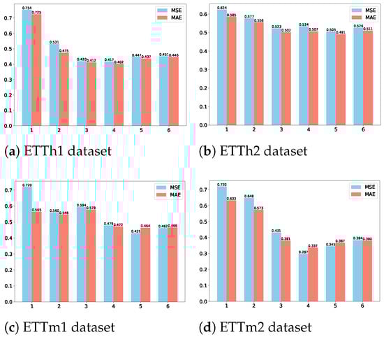
Figure 3. Effect of different scale values K on forecasting performance across four datasets. The x-axis shows the scale K, and the y-axis shows the mean squared error (MSE).

4.7. Visualization Analysis

4.7.1. Trend Spatio-Temporal Embedding Visualization

t-SNE is also employed to visualize the multi-scale spatio-temporal feature representations across the four datasets. Taking the trend spatio-temporal features as an example, the representations across all scales are projected into a two-dimensional space, as illustrated in Figure 4. It can be clearly observed that the some spatio-temporal embedding of trend features from different scales tend to cluster into distinct regions. Moreover, some multi-scale features still map to the same region (see the red circles in the figure), which can be attributed to the overlap present among spatio-temporal features across different scales. Overall, this further validates that multi-scale analysis can provide valuable insights into analyzing load time series from multiple perspectives, which enables a deeper understanding of the underlying patterns for enhanced prediction. A visualization of the learned trend (i.e., $\mathbf{S}trend$) and seasonal (i.e., $\mathbf{S}season$) features is provided. The results reveal clear and distinguishable patterns for both components. Moreover, the ablation studies indicate that the trend and seasonal components provide complementary information for forecasting, and their interaction contributes substantially to performance gains.

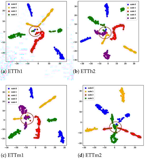
Figure 4. Trend spatio-temporal embedding visualization.The t-SNE was run with a perplexity of 10, and the random seed was set to 44 in the implementation.

4.7.2. Adjacency Matrix Visualization

In addition, the learned adjacency matrices for the trend and seasonal graphs are visualized on the ETTh1 dataset. Figure 5 shows the trend adjacency matrix (${\mathbf{A}}_{trend}$) and seasonal adjacency matrix (${\mathbf{A}}_{season}$) for a randomly selected time step. It can be observed that the two matrices exhibit low similarity. This difference indicates that the two graphs capture complementary information, supporting the effectiveness of multi-scale spatio-temporal modeling in MTSGNN.

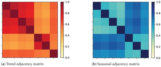
Figure 5. Trend and seasonal adjacency matrix visualization on the ETTh1 dataset.

4.8. Complexity Analysis

The computational complexity of MTSGNN is analyzed under the assumption that the hidden dimensionality across all layers is $D_{max}$. Let L denote the sequence length, N the number of sensors (or time series), and K the number of temporal scales. For a single scale, the main computational cost arises from three components: (i) temporal feature extraction, which requires $\mathcal{O}\left(L{D}_{max}^2\right)$, (ii) graph convolution to capture spatial dependencies, with cost $\mathcal{O}(N^2{D}_{max}+N{D}_{max}^2)$, and (iii) scale-wise trend and seasonal aggregation, costing $\mathcal{O}\left(N{D}_{max}^2\right)$. Combining these, the total complexity per scale is $\mathcal{O}\left(L{D}_{max}^2+N{D}_{max}^2+N^2{D}_{max}+N{D}_{max}^3\right)$. Considering all K scales, the overall complexity for temporal–spatial processing and scale-wise aggregation is $\mathcal{O}\left(K(L{D}_{max}^2+N{D}_{max}^2+N^2{D}_{max}+N{D}_{max}^3)\right)$. The final attention-based trend–seasonal fusion has complexity $\mathcal{O}\left(N^2{D}_{max}\right)$, which is relatively minor. Therefore, the total computational complexity of MTSGNN can be summarized as $\mathcal{O}\left(K(L{D}_{max}^2+N{D}_{max}^2+N^2{D}_{max}+N{D}_{max}^3)\right)$.

4.9. Training and Inference Time

As shown in Table 4, although MTSGNN exhibits slightly higher computational complexity than PathFormer, it achieves shorter training time due to the carefully designed modules that facilitate faster convergence. As noted in the Introduction, short-term load forecasting typically requires predictions over horizons ranging from several minutes to one week. Under this setting, the inference times of both models are sufficiently small to meet the real-time requirements of practical applications.

Table 4. Comparison of training and inference time on the ETTh1 dataset.

Methods	Complexity	Training Time (s)	Inference Time (s)
PathFormer	$\mathcal{O}\left(KN(L^2{D}_{max}+L{D}_{max}^2)\right)$	1034.23	3.09
MTSGNN (Ours)	$\mathcal{O}\left(K(L{D}_{max}^2+N{D}_{max}^2+N^2{D}_{max}+N{D}_{max}^3)\right)$	503.15	3.03

5. Conclusions

This work presents a novel end-to-end multi-scale trend–seasonal graph neural network (MTSGNN) for electricity load forecasting. By integrating the Hawkes process and multi-scale decomposition, MTSGNN captures temporal decay effects and complementary trend–seasonal patterns, while graph modeling exploits inter-variable dependencies. Experiments on six real-world datasets demonstrate consistent improvements over strong baselines, with up to 9.17% reduction in MSE. These results highlight the effectiveness of modeling multi-scale temporal structures and sensor relationships for accurate multivariate time series forecasting.

Despite these promising results, MTSGNN has been primarily evaluated on electricity datasets, and its applicability to other domains (e.g., traffic, finance) remains to be explored. Additionally, external factors such as economic indicators were not incorporated. Future work will focus on integrating exogenous information, extending to other domains, and enabling adaptive real-time forecasting.

References

- Zhuang, W.; Pan, G.; Gu, W.; Zhou, S.; Hu, Q.; Gu, Z.; Wu, Z.; Lu, S.; Qiu, H. Hydrogen economy driven by offshore wind in regional comprehensive economic partnership members. Energy Environ. Sci. 2023, 16, 2014–2029. [Google Scholar] [CrossRef]
- Liu, H.; Zhou, S.; Gu, W.; Zhuang, W.; Gao, M.; Chan, C.; Zhang, X. Coordinated planning model for multi-regional ammonia industries leveraging hydrogen supply chain and power grid integration: A case study of Shandong. Appl. Energy 2025, 377, 124456. [Google Scholar] [CrossRef]
- Yang, F.; Meng, F.; Qiu, Y.; Zhou, S.; Zhuang, W.; Liu, H.; Gu, W.; Yang, Y. Multi-dimensional assessment of decarbonization technologies and pathways in China’s iron and steel industry: An energy-process chain perspective. Energy Strategy Rev. 2025, 61, 101810. [Google Scholar] [CrossRef]
- Alfares, H.K.; Nazeeruddin, M. Electric load forecasting: Literature survey and classification of methods. Int. J. Syst. Sci. 2002, 33, 23–34. [Google Scholar] [CrossRef]
- Kuster, C.; Rezgui, Y.; Mourshed, M. Electrical load forecasting models: A critical systematic review. Sustain. Cities Soc. 2017, 35, 257–270. [Google Scholar] [CrossRef]
- L’Heureux, A.; Grolinger, K.; Capretz, M.A. Transformer-based model for electrical load forecasting. Energies 2022, 15, 4993. [Google Scholar] [CrossRef]
- Yalcinoz, T.; Eminoglu, U. Short term and medium term power distribution load forecasting by neural networks. Energy Convers. Manag. 2005, 46, 1393–1405. [Google Scholar] [CrossRef]
- Haque, A.; Rahman, S. Short-term electrical load forecasting through heuristic configuration of regularized deep neural network. Appl. Soft Comput. 2022, 122, 108877. [Google Scholar] [CrossRef]
- Lindberg, K.; Seljom, P.; Madsen, H.; Fischer, D.; Korpås, M. Long-term electricity load forecasting: Current and future trends. Util. Policy 2019, 58, 102–119. [Google Scholar] [CrossRef]
- Lee, C.M.; Ko, C.N. Short-term load forecasting using lifting scheme and ARIMA models. Expert Syst. Appl. 2011, 38, 5902–5911. [Google Scholar] [CrossRef]
- Dong, X.; Deng, S.; Wang, D. A short-term power load forecasting method based on k-means and SVM. J. Ambient. Intell. Humaniz. Comput. 2022, 13, 5253–5267. [Google Scholar] [CrossRef]
- Wang, Y.; Sun, S.; Chen, X.; Zeng, X.; Kong, Y.; Chen, J.; Guo, Y.; Wang, T. Short-term load forecasting of industrial customers based on SVMD and XGBoost. Int. J. Electr. Power Energy Syst. 2021, 129, 106830. [Google Scholar] [CrossRef]
- Yao, X.; Fu, X.; Zong, C. Short-term load forecasting method based on feature preference strategy and LightGBM-XGboost. IEEE Access 2022, 10, 75257–75268. [Google Scholar] [CrossRef]
- Sun, L.; Qin, H.; Przystupa, K.; Majka, M.; Kochan, O. Individualized short-term electric load forecasting using data-driven meta-heuristic method based on LSTM network. Sensors 2022, 22, 7900. [Google Scholar] [CrossRef]
- Li, D.; Sun, G.; Miao, S.; Gu, Y.; Zhang, Y.; He, S. A short-term electric load forecast method based on improved sequence-to-sequence GRU with adaptive temporal dependence. Int. J. Electr. Power Energy Syst. 2022, 137, 107627. [Google Scholar] [CrossRef]
- Zhao, Z.; Xia, C.; Chi, L.; Chang, X.; Li, W.; Yang, T.; Zomaya, A.Y. Short-term load forecasting based on the transformer model. Information 2021, 12, 516. [Google Scholar] [CrossRef]
- Kipf, T.N.; Welling, M. Semi-supervised classification with graph convolutional networks. arXiv 2016, arXiv:1609.02907. [Google Scholar]
- Zhuang, W.; Fan, J.; Xia, M.; Zhu, K. A multi-scale spatial–temporal graph neural network-based method of multienergy load forecasting in integrated energy system. IEEE Trans. Smart Grid 2023, 15, 2652–2666. [Google Scholar] [CrossRef]
- Liu, S.; Wu, C.; Zhu, H. Graph neural networks for learning real-time prices in electricity market. arXiv 2021, arXiv:2106.10529. [Google Scholar] [CrossRef]
- Wei, C.; Pi, D.; Ping, M.; Zhang, H. Short-term load forecasting using spatial-temporal embedding graph neural network. Electr. Power Syst. Res. 2023, 225, 109873. [Google Scholar] [CrossRef]
- Wu, H.; Xu, J.; Wang, J.; Long, M. Autoformer: Decomposition transformers with auto-correlation for long-term series forecasting. Adv. Neural Inf. Process. Syst. 2021, 34, 22419–22430. [Google Scholar]
- Wang, S.; Wu, H.; Shi, X.; Hu, T.; Luo, H.; Ma, L.; Zhang, J.Y.; Zhou, J. Timemixer: Decomposable multiscale mixing for time series forecasting. arXiv 2024, arXiv:2405.14616. [Google Scholar] [CrossRef]
- Saeed, F.; Rehman, A.; Shah, H.A.; Diyan, M.; Chen, J.; Kang, J.M. SmartFormer: Graph-based transformer model for energy load forecasting. Sustain. Energy Technol. Assess. 2025, 73, 104133. [Google Scholar] [CrossRef]
- Hochreiter, S.; Schmidhuber, J. Long short-term memory. Neural Comput. 1997, 9, 1735–1780. [Google Scholar] [CrossRef] [PubMed]
- Luo, S.; Wang, B.; Gao, Q.; Wang, Y.; Pang, X. Stacking integration algorithm based on CNN-BiLSTM-Attention with XGBoost for short-term electricity load forecasting. Energy Rep. 2024, 12, 2676–2689. [Google Scholar] [CrossRef]
- Jin, M.; Zhou, X.; Zhang, Z.M.; Tentzeris, M.M. Short-term power load forecasting using grey correlation contest modeling. Expert Syst. Appl. 2012, 39, 773–779. [Google Scholar] [CrossRef]
- Ediger, V.Ş.; Akar, S.; Uğurlu, B. Forecasting production of fossil fuel sources in Turkey using a comparative regression and ARIMA model. Energy Policy 2006, 34, 3836–3846. [Google Scholar] [CrossRef]
- Taylor, J.W. Short-term electricity demand forecasting using double seasonal exponential smoothing. J. Oper. Res. Soc. 2003, 54, 799–805. [Google Scholar] [CrossRef]
- Taylor, J.W. Triple seasonal methods for short-term electricity demand forecasting. Eur. J. Oper. Res. 2010, 204, 139–152. [Google Scholar] [CrossRef]
- Gao, M.; Zhou, S.; Gu, W.; Wu, Z.; Liu, H.; Zhou, A.; Wang, X. MMGPT4LF: Leveraging an optimized pre-trained GPT-2 model with multi-modal cross-attention for load forecasting. Appl. Energy 2025, 392, 125965. [Google Scholar] [CrossRef]
- Cui, C.; He, M.; Di, F.; Lu, Y.; Dai, Y.; Lv, F. Research on power load forecasting method based on LSTM model. In Proceedings of the 2020 IEEE 5th Information Technology and Mechatronics Engineering Conference (ITOEC), Chongqing, China, 12–14 June 2020; IEEE: Piscataway, NJ, USA, 2020; pp. 1657–1660. [Google Scholar]
- Zhang, Z.; Liu, J.; Pang, S.; Shi, M.; Goh, H.H.; Zhang, Y.; Zhang, D. General short-term load forecasting based on multi-task temporal convolutional network in COVID-19. Int. J. Electr. Power Energy Syst. 2023, 147, 108811. [Google Scholar] [CrossRef]
- Luo, H.; Zhang, H.; Wang, J. Ensemble power load forecasting based on competitive-inhibition selection strategy and deep learning. Sustain. Energy Technol. Assess. 2022, 51, 101940. [Google Scholar] [CrossRef]
- Shi, H.; Xu, M.; Li, R. Deep learning for household load forecasting—A novel pooling deep RNN. IEEE Trans. Smart Grid 2017, 9, 5271–5280. [Google Scholar] [CrossRef]
- Fan, J.; Zhuang, W.; Xia, M.; Fang, W.; Liu, J. Optimizing attention in a Transformer for multihorizon, multienergy load forecasting in integrated energy systems. IEEE Trans. Ind. Inform. 2024, 20, 10238–10248. [Google Scholar] [CrossRef]
- Wu, D.; Lin, W. Efficient residential electric load forecasting via transfer learning and graph neural networks. IEEE Trans. Smart Grid 2022, 14, 2423–2431. [Google Scholar] [CrossRef]
- Wang, Y.; Rui, L.; Ma, J. A short-term residential load forecasting scheme based on the multiple correlation-temporal graph neural networks. Appl. Soft Comput. 2023, 146, 110629. [Google Scholar] [CrossRef]
- Mansoor, H.; Gull, M.S.; Rauf, H.; Khalid, M.; Arshad, N. Graph Convolutional Networks based short-term load forecasting: Leveraging spatial information for improved accuracy. Electr. Power Syst. Res. 2024, 230, 110263. [Google Scholar] [CrossRef]
- Cleveland, R.B.; Cleveland, W.S.; McRae, J.E.; Terpenning, I. STL: A seasonal-trend decomposition. J. Off. Stat. 1990, 6, 3–73. [Google Scholar]
- Wang, H.; Li, S.; Wang, T.; Zheng, J. Hierarchical Adaptive Temporal-Relational Modeling for Stock Trend Prediction. In Proceedings of the IJCAI, Montreal, QC, Canada, 19–27 August 2021; pp. 3691–3698. [Google Scholar]
- Marmolin, H. Subjective MSE measures. IEEE Trans. Syst. Man, Cybern. 1986, 16, 486–489. [Google Scholar] [CrossRef]
- Chen, P.; Zhang, Y.; Cheng, Y.; Shu, Y.; Wang, Y.; Wen, Q.; Yang, B.; Guo, C. Pathformer: Multi-scale transformers with adaptive pathways for time series forecasting. arXiv 2024, arXiv:2402.05956. [Google Scholar] [CrossRef]
- Cho, K.; Van Merriënboer, B.; Gulcehre, C.; Bahdanau, D.; Bougares, F.; Schwenk, H.; Bengio, Y. Learning phrase representations using RNN encoder-decoder for statistical machine translation. arXiv 2014, arXiv:1406.1078. [Google Scholar] [CrossRef]
- Veličković, P.; Cucurull, G.; Casanova, A.; Romero, A.; Lio, P.; Bengio, Y. Graph attention networks. arXiv 2017, arXiv:1710.10903. [Google Scholar]
- Wu, Z.; Pan, S.; Long, G.; Jiang, J.; Chang, X.; Zhang, C. Connecting the dots: Multivariate time series forecasting with graph neural networks. In Proceedings of the 26th ACM SIGKDD International Conference on Knowledge Discovery & Data Mining, San Diego, CA, USA, 23–27 August 2020; pp. 753–763. [Google Scholar]
- Kingma, D.P. Adam: A method for stochastic optimization. arXiv 2014, arXiv:1412.6980. [Google Scholar]
Disclaimer/Publisher’s Note: The statements, opinions and data contained in all publications are solely those of the individual author(s) and contributor(s) and not of MDPI and/or the editor(s). MDPI and/or the editor(s) disclaim responsibility for any injury to people or property resulting from any ideas, methods, instructions or products referred to in the content. |
© 2025 by the authors. Licensee MDPI, Basel, Switzerland. This article is an open access article distributed under the terms and conditions of the Creative Commons Attribution (CC BY) license (https://creativecommons.org/licenses/by/4.0/).