Abstract
Drug delivery from cylindrical tablets of arbitrary dimensions is discussed here, using the analytical solution of diffusion equation. Utilizing dimensionless quantities, we show that the release profiles are determined by a unique parameter, represented by the aspect ratio of the cylindrical formulation. Fractional release curves are presented for different values of the aspect ratio, covering a range of many orders of magnitude. The corresponding release profiles lie in between the two opposite limits of release from thin slabs and two-dimensional radial release, pertinent to the cases of thin and long cylinders, respectively. In a quest for a part of the delivery process closer to a zero-order release, the release rate is calculated, which is found to exhibit the typical behavior of purely diffusional release systems. Two simple fitting formulae, containing two parameters each, are considered to approximate the infinite series of the exact solution: The stretched exponential (Weibull) function and a recently suggested expression interpolating between the correct time dependencies at the initial and final stages of the process. The latter provides a better fitting in all cases. The variation of the fitting parameters with the aspect ratio of the device is presented for both fitting functions. We also calculate the characteristic release time, which is found to correspond to an amount of fractional release between 64% and around 68% depending on the cylindrical aspect ratio. We discuss how the last quantities can be used to estimate the drug diffusion coefficient from experimental release profiles and apply these ideas to published drug delivery data.
1. Introduction
Mathematical modeling of drug delivery systems not only elucidates the underlying release mechanisms but also facilitates the design of pharmaceutical formulations with desired release characteristics, thus reducing the effort and the cost of time consuming experimental trials. As a result, both empirical and mechanistic theoretical models have been developed, representing an important area in the field of controlled drug release. Various delivery devices, where different mechanisms dominate the release process, are described through either analytical or numerical solutions of relevant models [1,2,3,4,5,6]. Nowadays, the increased demand for a precise control of release kinetics, achieved using more sophisticated materials and technologies [7,8], renders modeling even more significant.
Recent mathematical models, for example, investigate coupled reaction–diffusion release mechanisms. In this case, the release process is described through diffusion of the bioactive compounds within the matrix, but various reversible or irreversible chemical reactions are involved as well. Irreversible binding reactions of diffusing drug molecules to matrix components have been examined for monolithic and core-shell systems of various shapes [9], for multilayer spheres [10], and for inhomogeneous spherical carriers with arbitrary spatial variation in the drug diffusion coefficient and the reaction rate constant [11]. Other theoretical studies discuss conjugated polymer-drug systems where the drug is initially covalently linked to the polymer matrix through labile bonds, which can be cleaved by various chemical reactions and then the liberated drug molecules are able to diffuse and be released from the carrier [12,13]. Models have been developed for affinity-based systems, where the diffusing drug molecules bind transiently through reversible, non-covalent interactions to ligands attached within the matrix [14,15]. Polymeric surface erosion and simultaneous drug diffusion have been considered for spherical capsules [16] as well as for devices of various geometries where polymer-drug binding reactions are also included [17]. Further, more complicated release mechanisms like swelling [18] are numerically modeled [19,20], even in the case of formulations with complex dome-shaped matrices of cylindrical symmetry exhibiting a convex and a concave opposite faces [21], and hydrogels can be rationally designed for optimized drug delivery [22].
Diffusion is the simplest release mechanism, but it is almost always present in the release process, either alone or in combination with other mechanisms. Thus, purely diffusional drug release still attracts research interest, especially for complicated situations involving composite, inhomogeneous, or porous devices [23,24,25,26,27,28,29], or in cases where the carriers exhibit a size distribution [30]. Moreover, release data obtained by considering merely diffusion have been used to test methods and procedures in the analysis of numerical or experimental release profiles [31,32].
In diffusion-controlled release from homogeneous matrices with a uniform initial drug loading, there exist analytical solutions of the corresponding mathematical problem described by Fick’s second law [33,34,35]. The obtained exact expressions of the release profiles are in the form of infinite series, rendering them not very practical for the description of various experimental or numerical data. As a result, various approximations of the release kinetics by simple analytical formulae have been considered. One such relation that is very popular is the power-law [36,37], which has been broadly applied in experimental investigations due to its simplicity. Another frequently used approximation is the Weibull (or stretched exponential) function [38,39,40,41]. The power-law efficiently describes the first part of release (up to 60%), while the stretched exponential is able to approximate the complete release profile. The latter expression has been used to model a number of experimentally measured [42,43,44] or numerically derived [45,46] release kinetics.
Cylindrical devices contain two size parameters, the height (or length) and radius, which can be varied independently, thus exhibiting richer release behavior as compared to other formulations, like spheres or slabs, characterized by a single size parameter. The latter cases are described by universal release profiles, as can be seen using dimensionless quantities [47]. In these cases, in particular, different systems exhibit identical release curves apart from a rescaling of time by a factor equal to the drug diffusion coefficient over the squared size of the device. On the contrary, cylindrical carriers produce release profiles that depend on the relative ratio of their two size parameters, like the aspect ratio of the system. Even richer behavior can be obtained by ellipsoidal drug delivery carriers [48,49,50], which, in general, contain three size parameters and thus the resulting release profiles will depend on two relative ratios of the lengths of their semi-axes.
Here, we elaborate on diffusional drug delivery from cylindrical-shaped formulations. The dependence of release profiles and release rates on the cylinder’s aspect ratio is explicitly presented. In order to facilitate a quantitative description of experimental release data, we have fitted the exact drug delivery profiles, provided through the known infinite series solution of diffusion equation, with simpler empirical relations. The latter can be used to approximate the corresponding release profiles. The dependence of the fitting parameters of these empirical formulae on the geometrical (height and radius) and physicochemical (diffusion coefficient) properties of the carrier is obtained. Further, the characteristic release time is discussed and we show how it can be used to estimate the drug diffusion coefficient, a not so easily accessible microscopic parameter, from experimental data. We demonstrate this procedure using published experimental release profiles. The presented results can be useful for designing cylindrical delivery devices and nanocarriers with the desired release kinetics.
In Section 2, we start with the known solution for the fractional release profiles of cylindrical matrices and use dimensionless variables to simplify the subsequent analysis. Then, the influence of the device’s aspect ratio on the release profiles and the corresponding release rates are shown. Section 3 presents fittings of the exact fractional release with two approximating functions (the stretched exponential and a recently introduced interpolating formula) and the dependence of the derived fitting parameters on the device dimensions, and the drug diffusion coefficient is examined. Finally, the characteristic release time and its usefulness for estimating drug diffusion coefficients from release experiments is discussed in Section 4. Section 5 concludes our study.
2. Fractional Release Profiles and Release Rates
2.1. Theoretical Background: Exact Results from the Solution of Diffusion Equation in Dimensionless Form
We consider a cylindrical carrier of height H and radius R, homogeneously loaded with an amount of drug equal to . Drug molecules diffuse with a diffusion coefficient D through the matrix and exit the formulation when they reach the boundary surfaces. The latter consist of the two circular bases of the cylinder and its lateral surface. In this case, the solution of diffusion equation, using sink boundary conditions, provides the fractional release [34,51]:
where stands for the amount of drug released at time t ( is the fractional release at t) and corresponds to the root of the zero-order Bessel function . The first sum over m represents a sum over all roots of the equation , whereas the second sum runs over all non-negative integers n.
Considering the cylinder’s aspect ratio as its height divided over its diameter
and using the dimensionless time
then the fractional release of Equation (1) reads
This result shows that the release profiles from cylinders depend on a single parameter, the aspect ratio A. Cylindrical tablets with different heights and radii but having the same aspect ratio exhibit identical release profiles apart from a rescaling of time by a factor . The drug diffusion coefficient appears just in this rescaling of time, while the shape of release profile is determined exclusively by the ratio of the two size parameters.
The drug delivery profiles provided by Equation (4) are discussed in the next subsection. Before that, two limiting cases of this problem will be considered:
- Flat disks, where the height of the cylinder is significantly smaller than its radius ( or ). In this situation, the release from cylinder’s lateral surface can be ignored, as it is substantially smaller compared to the release from the two circular bases, which exhibit a much larger area for the escape of drug molecules. Then, Equation (1) reduces to the corresponding result describing release from a thin slab of thickness H [33]:
- Long cylindrical rods, where the cylinder’s height is much larger than its radius ( or ). In this case, the release from the two circular bases can be ignored since the drug molecules exit mainly through the much larger boundary area of the lateral surface of the cylinder. Then, Equation (1) ends up being the result of a two-dimensional radial release from a disc of radius R [33]:Here, the natural dimensionless time isand the resulting fractional release of Equation (7), which does not depend on any parameter, isHowever, in order to compare this limiting case with the general description of cylindrical release discussed in this work, we consider the dimensionless time of Equation (3), and then Equation (7) yields the A-dependent formulaThe last two equations are connected through the transformation of their independent variables
2.2. Dependence of Fractional Release Profiles on the Aspect Ratio
Release profiles obtained from Equation (4) for different values of the aspect ratio A, ranging from to , as a function of the dimensionless time are plotted by continuous lines in Figure 1, both in linear (top) and logarithmic (bottom) time scale. The larger the aspect ratio, the faster the release in dimensionless time units. However, in real time units, the rescaling of time according to Equation (3) should be considered too.
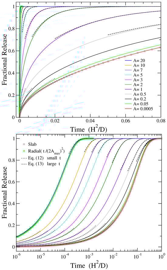
Figure 1.
Release profiles , given by Equation (4), in (top) linear and (bottom) logarithmic time scale (solid lines) for different values of the aspect ratio A as indicated in the upper plot. Squares show the corresponding release from slabs, provided by Equation (6), expected to hold for . Circles represent radial release from two-dimensional disks, provided by Equation (9), with the abscissa scaled by [see Equation (11)], expected to hold for . Dotted and dashed lines depict the short time and long time approximations of release for each particular case, provided by Equations (12) and (13), respectively.
For comparison with the two extreme values of A presented in this plot ( and ), the limiting cases of release from a slab, provided by Equation (6), and radial release from a disc, as provided by Equation (9) while taking into account the scaling of the independent variable by as indicated in Equation (11), are also depicted by open squares and circles, respectively. As can be seen from Figure 1, the release from slab (radial release) coincides with that obtained for the smaller (larger) value of the aspect ratio considered in this work.
For short times, , the fractional release of Equation (4) varies as the square root of time [36]:
This formula reduces to the corresponding expressions for a thin slab, () when , and for a two-dimensional radial release, (), when . Dotted lines in Figure 1 show the result of Equation (12) for the corresponding values of A presented in the plot. It can be seen that this equation describes well the initial part of release in all cases.
For relatively long times, the term with the smallest exponent dominates the sum of Equation (4), resulting in
where is the first root of the zero-order Bessel function , which approximately equals to 2.4048 [52]. This formula does not provide the correct limiting values for slabs, , when and for radial release, , when . This is due to the differences in the preexponential coefficients from 8 in the former case and from 4 in the latter case. The deviation from the correct limits is larger when . To obtain the right behavior in these cases, one should first consider the corresponding limit of the aspect ratio, or , and then the limit of large . The predictions of Equation (13) are depicted with dashed lines in Figure 1, providing a rather good description of the late part of release, except for the smallest values of A examined here, for the reason explained previously.
2.3. Release Rates for Different Aspect Ratios
The release rate can be directly derived though differentiation of Equation (4), yielding
This equation provides the correct limiting expressions for the rates in the cases of release from slabs and radial release, respectively. In particular, when , the first term in the preexponential large parenthesis and the first term in the exponent can be ignored. Then, taking into account that , Equation (14) leads to the release rate , which coincides with the rate from a slab as can be easily seen by the derivative of Equation (6). At the opposite limit of , the corresponding second terms in the preexponential factor and the exponent of Equation (14) can be ignored, and considering that , one obtain the rate , providing the rate of radial release as obtained through derivation of Equation (10).
Figure 2 presents the variation of release rate with the amount of fractional release, instead of time. This representation is preferable [53,54] than the time dependence of the release rate, as it directly demonstrates the range of fractional release where the delivery is closer to a zero-order process, i.e., a constant release rate. Further, it facilitates the comparison of the corresponding release rates from cylinders of different aspect ratios, where the drug release occurs in different time scales.
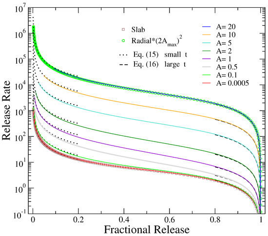
Figure 2.
Release rate as a function of fractional release for different values of A as shown in the label (solid lines). The corresponding plots for the cases of release from slabs, by differentiating Equation (6), and radial release from disks, through the derivative of Equation (9) and multiplication by , are depicted by open squares and circles, respectively. Dotted lines represent the short-time behavior of Equation (15) and dashed lines the long-time behavior of Equation (16).
As can be seen from Figure 2, the release rate in all cases exhibits the typical diffusional behavior [55]. It obtains extremely high values at the beginning of release (actually Equation (14) diverges at ), initially drops very fast by many orders of magnitude, and then shows a slower decay in the regime roughly between 20% and 80% of fractional release. In this range of fractional release, the process is as close it can be to a zero-order release. In the last part of release, the rate declines linearly to zero when all drug molecules have diffused out of the formulation and the process is ended. The limiting cases of slab (flat disc), obtained from the derivative of Equation (6), and two-dimensional radial release, derived through differentiation of Equation (9) multiplied by due to Equation (11), are also presented in Figure 2 for comparison with the results of the smallest and largest aspect ratios considered here, showing a perfect coincidence. To quantify how close the results depicted in Figure 2 in the regime of the slowest decay (between 20–80% of release) are to a zero-order release, we have calculated the slopes of the logarithms of the rates (in dimensionless times) versus fractional release in this regime. The smaller slope (on absolute value, since the slopes are negative) is obtained for the smaller value of A, in the limit of release from slabs. As the aspect ratio increases up to A at around 1, the absolute value of the slope increases. Then, as the aspect ratio continues to increase towards the limit of radial release, the absolute value of the slope decreases with A.
Using the approximations at short and long times discussed in previous subsection, simple expressions can be derived for the dependence of on fractional release . In particular, for , Equation (12) yields that the release rate is inversely proportional to . Then, substituting as a function of from the same relation, one obtains
The last result is plotted by dotted lines in the left part of Figure 2 for the different values of A shown in the figure. This dependence describes accurately the initial part of release rate, corresponding to short times.
For the late part of release, Equation (13) shows that the release rate is proportional to . Using the same relation, this exponential can be expressed as a function of , resulting in
Dashed lines in the right part of Figure 2 depict this linear drop to zero, which describes very well the late part of the process. The accurate description holds even for the limiting cases of and , despite the discrepancy mentioned in the previous subsection concerning the time dependence of fractional release in these limits. The reason for this is that the coefficient causing this error has been canceled during the substitution of the time-exponential term of the release rate when expressed as a function of fractional release. Indeed, for flat disks, Equation (6) indicates that at relatively long times, , while for long rods, Equation (10) indicates at long times. Then, the release rates are and , respectively. These results coincide with the corresponding limits of Equation (16) for and .
3. Fitting with Simpler Empirical Functions
Equation (4) describes the exact release profile of a cylindrical device when diffusion is the main mechanism of drug delivery. However, the infinite series, typically appearing in the solution of Fick’s second law, makes this exact result complicated and inconvenient for use in corresponding experimental studies, even more so in this case of cylindrical release, where a double sum appears and the one is over the roots of Bessel function.
Simpler empirical expressions, like the power-law [36,37], provide more efficient descriptions of release profiles. However, the behavior of the polynomial function at large times makes the latter formula inadequate in describing the late part of fractional release, restricting its use for up to 60% of the release profile. Another simple, two-parameter relation that can qualitatively describe the whole process is the stretched exponential, or Weibull, function [56]:
This function starts from zero and saturates to one at larger times, as expected for a fractional release profile in cases where the entirety of the drug can exit the formulation. It contains two parameters: the stretched exponential time and the stretched exponent b. The last equation has been frequently used to fit fractional release data.
It has been noted that even though Equation (17) has the proper limiting values both at the beginning and at the end of the release process, it does not exhibit the correct temporal dependence in the neighborhood of these limits [57]. In particular, it does not increase as the square root of time at short times and also does not approach unity as a simple exponential at relatively long times, as with all diffusional release problems (see, for example, Equations (12) and (13), respectively, in our case of release from cylinders). This inefficiency of the stretched exponential function to properly describe the initial and the last part of release has been also observed when the dynamics of the fraction of drug molecules close to the release boundary were examined [58]. Slater and collaborators have suggested another two-parameter formula for describing fractional release profiles, which interpolates between the correct limiting behaviors at the beginning and at the end of a purely diffusional delivery process [57]:
The two time parameters and of this empirical formula correspond to the initial diffusion time and the longest relaxation time of the diffusional release [57].
Here, we have used both the stretched exponential, Equation (17), and the interpolating, Equation (18), functions in order to fit the infinite series of the exact result providing the fractional release from a cylindrical carrier. Our purpose is to present approximating, but accurate and convenient, simple empirical formulae that can be used to describe drug release from devices of cylindrical shape with arbitrary sizes. To this end, we have fitted release profiles obtained from Equation (4) for various aspect ratios, covering the whole range between the limits of flat disks () and long cylinders (), and present the dependence of the fitting parameters on the aspect ratio. Then, using Equation (3), we can restore normal units and thus provide the dependence of the fitting parameters of the empirical functions on the dimensions of the cylinder and the drug diffusion coefficient.
Figure 3 shows a representative fitting. The exact result of Equation (4) for is depicted by open circles, while the continuous lines are fittings with Equations (17) and (18). The inset shows the same plot in logarithmic time scale in order to access the initial part of release, which is not distinguished in the main graph. The fitting with the interpolating formula (red curve) is very robust, contrary to the stretched exponential function where the stretched exponent b is sensitive to the fitted data points of fractional release. This sensitivity of parameter b has been already noted in earlier studies [32,59]. For this reason, two different fittings are presented in Figure 3 regarding the Weibull fit: The blue and green curves are obtained when the fitting emphasizes more the longer- or shorter-time data points, respectively. The dashed orange curve provides a compromise of this situation, corresponding to the average values of the fitting parameters obtained in the latter two cases. The emphasis of the blue and green curves on different stages of release can be clearly seen from the different stretched exponential fittings in the figure.
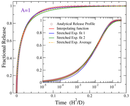
Figure 3.
Solid lines depict fittings of the analytical release profile of Equation (4) for aspect ratio (shown by open circles) with the stretched exponential and the interpolating functions of Equations (17) and (18), respectively. Red curve presents the fitting with the interpolating function. Blue and green lines show fittings of the Weibull function with different emphasis on the late- or early-time data points, respectively. Dashed orange curve represents the Weibull function with parameters given by the average values of the corresponding parameters obtained through these two fittings of the blue and green lines.
Overall the interpolating formula provides a better fitting than the stretched exponential function in all cases for all different values of A examined here. In general, the sum of the squared differences between the exact and the fitting values divided over the total number of data points is at least two order of magnitudes smaller for the interpolating function as compared to the stretched exponential fittings. In particular, the mean square error across the full release curve from 0 to 1 is of the order of ∼– in the fitting with the interpolating formula and ∼ in the Weibull fitting. The fitting errors do not exhibit a systematic dependence on A. The superiority of the interpolating function in regards the fitting of diffusional release from homogeneously loaded matrices has also been demonstrated in Ref. [31] for the cases of drug delivery from slabs, two-dimensional disks, and spheres. Below, the dependence of the fitting parameters on the aspect ratio A is discussed for both fitting functions.
3.1. Fitting Parameters of the Interpolating Function
Solid symbols in Figure 4 show the variation in the fitting parameters and of Equation (18) with the cylindrical carrier’s aspect ratio. The former parameter characterizes the early-time behavior of release, while the latter characterizes the late-time behavior. Both fitting parameters have dimensions of time, as can be readily seen from Equation (18). As already mentioned, the fitting values of these parameters are very robust with regard to the fitted data points of the release profile. In particular, in both plots of Figure 4, there are two sets of parameter values: one obtained with more emphasis on the initial part of release and the other with more emphasis on data points of the later part. These two sets are practically indistinguishable, but taking a careful look, one may notice very small differences in the heights of blue squares, reflecting the existence of two overlapping data sets.
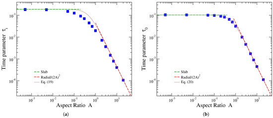
Figure 4.
Fitting parameters of the interpolating function, Equation (18), versus the aspect ratio A of the cylinder (blue solid symbols). (a) Early-time parameter and (b) late-time parameter . Green dashed lines at the left part of the plots show the corresponding parameter values for thin slabs, obtained in the limit . Red dashed lines at the right part of the plots show the corresponding parameter values for radial release, applicable in the limit . Brown continuous line represents the interpolation between these two limiting cases, provided by Equations (19) and (20) for and , respectively.
The limiting values of the A dependence of parameters and can be obtained by the corresponding parameter values in the case of release from slabs and radial release from two-dimensional disks. Such results are presented in Table 3 of Ref. [31]. Regarding the early-time parameter , the corresponding fitting values for release from slabs and disks transformed to the dimensionless time units used here are and [31]. Thus, the expected limiting behaviors of are as follows: a constant value for and a dependence for , where Equation (11) has been taken into account in the latter case. These limits are shown by the green and red dashed lines, respectively, in Figure 4a. Considering a simple interpolation between these two limiting behaviors results in
This formula is shown by solid brown curve in Figure 4a. It describes accurately the fitting parameter for relatively small and large values of A, but it overestimates its values in the region for a factor of no more than about 2.
Concerning the late-time parameter , the corresponding fitting values considering release from thin slabs and two-dimensional disks are, in our dimensionless time units, and [31]. Therefore, is expected to tend to the constant value for , a result shown by a green dashed line in Figure 4b, and is expected to behave as for , a dependence depicted by a red dashed line in this figure. The continuous brown line in Figure 4b depicts the interpolating formula between these limits as follows:
which appear to accurately describe the dependence in the whole range of the aspect ratio values.
We summarize the obtained results in real-time units in order to facilitate their use for describing actual drug release data. In normal-time units the interpolating function reads
where the time parameters and are connected to the dimensionless and , respectively, through Equation (3). Taking this into account, along with the relations of Equations (19) and (20), it is suggested that diffusional release from a cylindrical tablet with height H, radius R, and diffusion coefficient D can be reasonably described by Equation (21), with parameter values
and
The aspect ratio from Equation (2) has been substituted in these relations. Equation (23) is expected to accurately provide the parameter , while Equation (22) is accurate when or , but it overestimates by a factor of up to about 2 the value of in the intermediate values of .
3.2. Fitting Parameters of the Stretched Exponential Function
Figure 5 presents the dependence of the stretched exponential fitting parameters (left) and b (right) on the aspect ratio. It has been mentioned that the stretched exponent b is quite sensitive to the fitted fractional release data. The bars in Figure 5b demonstrate the range of different values of b obtained, as different parts of the release profiles of Equation (4) are emphasized in the fitting. The upper (lower) values of these bars, shown by filled circles (diamonds), are obtained when less (more) focus is given at the early part of fractional release during the fitting; see, for example, the blue (green) fitted curve shown in Figure 3. The reported values of b in the literature usually emphasize more the late part of release [31,40,41]. In Figure 5a, two sets of fitted values are depicted by filled squares (as was the case for the time parameters of the interpolating function discussed previously), obtained from the two different fittings resulting in the values of b shown by circles and diamonds on the plot of Figure 5b. We see that, in contrast to the stretched exponent b, the fitting of the time parameter is more robust, as is the case for the time parameters and of the interpolating formula.
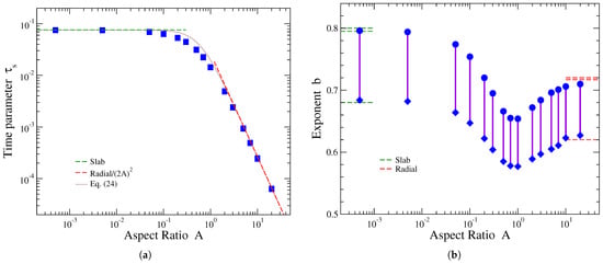
Figure 5.
Variation in the fitting parameters of the stretched exponential function, Equation (17), with the cylinder’s aspect ratio A. (a) Time parameter (blue solid symbols) and (b) stretched exponent b (bars with solid symbols at the ends, see text). Green dashed lines at the left part of the plots show the corresponding parameter values for thin slabs, obtained in the limit . Red dashed lines at the right part of the plots show the corresponding parameter values for radial release, applicable in the limit . Regarding the time parameter , the brown continuous line in (a) represents the interpolation between the two limiting cases, provided by Equation (24).
The dimensionless time parameter exhibits a monotonous decrease with the aspect ratio A, similarly to the behaviors of and presented in the previous subsection. In the limiting cases of release from slabs and radial release from disks, the corresponding fitting values of this parameter are [31,41] and [31,35], respectively. These results mean that for , the is expected to tend to the constant value 0.076, shown by the horizontal green dashed line in Figure 5a, while for , parameter should behave as , represented by red dashed line in this plot. We see from Figure 5a that these limits are nicely reproduced by the fitting parameter values. Interpolating between these limiting behaviors yields
This result is plotted by solid brown curve in Figure 5a. It provides a rather accurate description of the dependence of on A; in the worst case scenario, when the aspect ratio has values of the order of ∼, last equation overestimates by a factor less than 1.5.
Parameter b in Equation (17) is dimensionless and is therefore not affected by the chosen time units. Reported values for this fitting parameter in the case of release from slabs (two-dimensional disks), (), are 0.80 [41] and 0.795 [31] (0.72 [35] and 0.717 [31]) when the focus is more on the late part of release, while a smaller value of 0.68 (0.62) arises if more emphasis is given in the early stage of release. These results are represented by green (red) dashed lines in the left (right) part of Figure 5b. In between these limits, the stretched exponent b shows a non-monotonous dependence on A. As can be seen from Figure 5b, when A increases at first, b decreases from its limiting value . It then reaches a minimum value around and then increases up to the opposite limiting value .
A similar non-monotonous behavior, with the same characteristics as those of b, has been also observed regarding the variation of the exponent n of the power-law with the cylinder’s aspect ratio (see Figure 6 of Ref. [36]). Note that the aspect ratio in that work, , has been defined reversely than here, i.e., as . The minimum value of n () is obtained in that work when is within the range 1–2, which is in accordance with our minimum of b when our aspect ratio A is between 0.5 and 1. Furthermore, the limiting value of n is smaller when () as compared to that at (), in agreement with the results shown in Figure 5b where the limiting value of b is smaller when as compared to that when . This similarity in the behavior of the stretched exponent b and the power-law exponent n reinforces the linear correlation noticed in Ref. [42] (see Figure 3 in that work), where a large number of experimental data were fitted by these two empirical functions.
Summarizing the above results in real units, the stretched exponential function in dimensional time is
When this equation is used to describe fractional release profiles from cylindrical formulations, then considering Equations (3) and (24), the following approximating relation
provides the time parameter as a function of the device characteristics H, R, and D. This estimate is rather accurate for aspect rations or , whereas it slightly overestimates when by no more than 1.5 times.
The stretched exponent b is determined exclusively by the carrier’s aspect ratio, as shown in Figure 5b, where the upper limits of the bars can be considered for release profiles reaching substantial fractional release. This parameter does not depend on the individual values of the height and the radius of the cylindrical tablet, but only on their ratio. It does not depend on the drug diffusion coefficient as well.
4. Characteristic Release Time
It has been suggested that a single value of time can be used to characterize the time scale of a release process, which is provided by the integral of the complementary fractional release , where varies within the region 0–1 [13,31,47]
The time corresponds to a mean, or average, delivery time. The characteristic release time can be analytically obtained in the case of diffusional drug delivery from cylindrical matrices by substituting in Equation (27) the analytical solution presented in Section 2.1 and evaluating the resulting integral. Using dimensionless time units, represented in Equation (3), this calculation leads to [47]
providing as a function of the aspect ratio. The variation of with A, calculated through Equation (28), has been presented in Figure 2 of Ref. [47]. It has been verified here that identical results are obtained for the release time through direct numerical integration of Equation (27), using the release profiles like those plotted in Figure 1, for different values of A .
In real-time units, the characteristic release time, , is related to through
As we show below, this relation can be used for determining the drug diffusion coefficient from experimental release data, which can provide an estimate of the release time . Note that the diffusional release time of last equation provides a lower limit of the characteristic release time in some reaction–diffusion cylindrical release devices involving chemical reactions and diffusion of the bioactive substances.
It has been found that for purely diffusional release from simpler geometries, the amount of fractional release at time equal to the characteristic release time, , is around 65%. In particular, for thin slabs; for two-dimensional radial release; and [47] for spherical formulations. In conjugated polymer-drug slabs, this quantity lies approximately within the region 60–64%, depending on the value of the single parameter (dimensionless reaction rate constant) describing this process [13].
Here, we examine how the quantity varies with the aspect ratio of a cylindrical tablet in diffusion-controlled release. Note that , since a rescaling of time affects the x-axis of the release profile and the value of the characteristic time, according to Equation (29), but not the fractional amount of released drug at the characteristic release time as defined by the corresponding integral of Equation (27). In other words, this means that .
Figure 6 presents the variation of the amount of fractional release at the characteristic release time with the parameter A (solid diamonds). The limiting values for and , corresponding to the case of release from slabs and radial release from disks, are shown by green and red dashed horizontal lines, respectively. As can be seen from Figure 6, the quantity rises from about 64.4% up to 68.2% as the aspect ratio increases up to around one, and then for , it drops to a value close to 66.1%, the expected value for a two-dimensional radial release. This graph can be used to get an estimate of through experimentally measured release profiles, and then in conjunction with Equation (29), it can lead to an approximate calculation of the diffusion coefficient. This procedure is described in the next subsection.
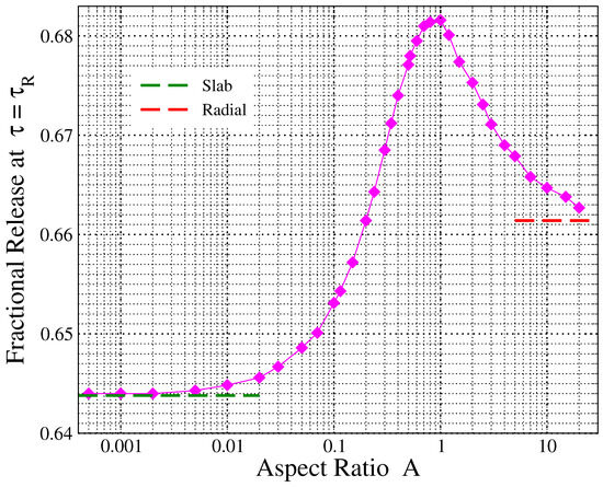
Figure 6.
Amount of fractional release at the characteristic release time, , as a function of the cylinder’s aspect ratio (filled symbols). Green and red dashed lines at the left and right part of the graph show the corresponding values for the case of thin slabs and radial release from disks, respectively.
4.1. Estimating Drug Diffusion Coefficients from Experimental Release Profiles of Cylindrically Shaped Formulations
The concept of characteristic release time and the amount of fractional release at this time, , can be used to estimate not easily accessed microscopic quantities like the drug diffusion coefficient [13,31,47]. Concerning the release process of interest here, the geometrical dimensions H and R, and thus the aspect ratio , of a cylindrical device can be easily measured in a relevant experiment. Then, computing the dimensionless release time for the given value of the aspect ratio and estimating the actual release time from the measured release profiles, this can lead to an estimate of the diffusion coefficient through Equation (29) as
Such an evaluation requires two steps:
- 1.
- Calculation ofThe dimensionless characteristic release time can be directly computed using Equation (28) for the given value of aspect ratio A. If such a calculation is not convenient, the can be alternatively obtained through the plot of Figure 2 of Ref. [47]. For , the dimensionless release time can be approximated by its corresponding value for thin slabs, , while for , it can be approximated by the two-dimensional radial release expression . A simple relation interpolating between these two limits can provide an approximation of the dependence of on the aspect ratio:If the aspect ratio lies in the region , then this formula would give a rough estimate of , overestimating its actual value. For a comparison of this simple approximating expression with the exact result of Equation (28), as well as the dependence of their difference on A, see Figure 2 of Ref. [47].
- 2.
- Estimate ofIf there exist sufficient experimental release data such that the area under the plot of the quantity (where, in this case, should have not been expressed as a percentage release, but varying in the interval ) can be accurately estimated, in which the release time is directly obtained by this integration, see Equation (27). In order to be reliable this calculation the release process should have been completed, i.e., the release curve has to be measured up to saturation, reaching its maximum value .In case there are no sufficient release data for obtaining the release time from the area under the plot of the complementary fractional release , then can be alternatively estimated from the data presented in Figure 6 as follows: Using the known value of the aspect ratio A, the amount of fractional release at , , can be obtained from this figure. Then, from the experimentally measured profile, the time at which this particular fraction of drug has been released can be estimated by linear interpolation of the nearby experimental data points immediately above and below of the desired amount of fractional release. For this purpose, it is necessary experimental data to be available for at least up to around 70% of released drug.
Deriving the dimensionless and the actual release times and from these two steps, a simple substitution in Equation (30) leads to an estimate of the value of diffusion coefficient. Note that experimental uncertainties in the tablet dimensions are included in the height H and the dimensionless release time (which is a function of A), while errors in the release data points are included in . In these cases, standard error propagation from Equation (30) provides the respective error of the calculated value of D. It is emphasized that in order to be relevant such an evaluation of D, diffusion should constitute the main release mechanism. Below, we apply this procedure to published experimental measurements of drug release profiles.
4.2. Demonstration of Diffusion Coefficient Evaluations from Experimental Release Data
We will demonstrate the method outlined above in 4 sets of diprophylline release measurements from cylindrical Kollidon SR-based matrices of different sizes published in Ref. [60]. For each of these sets, two different solvents were examined, 0.1 M HCl and phosphate buffer pH 7.4, resulting in 8 distinct release profiles. The experimental release data of interest are depicted by symbols in Figure 7, where the left (right) plot corresponds to exposure in 0.1 M HCl (phosphate buffer pH 7.4). In that work, it has been shown that diffusion was the main release mechanism in these experiments. At first, the authors were able to successfully fit several measured release profiles in different media with Equation (1) and obtained the diffusion coefficients from these fittings. Then, using these values of D, they predicted the effects of different tablet dimensions on the release kinetics considering purely diffusional release. Preparing formulations with these dimensions and measuring the corresponding release profiles in independent experiments showed a very good agreement with the theoretical predictions [60]. Here, instead of fitting Equation (1) with the release curves in order to obtain the drug diffusion coefficients, we use Equation (30) to estimate the corresponding values of D.
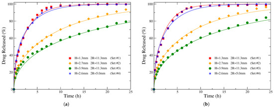
Figure 7.
Filled symbols and starts represent drug release profiles obtained experimentally in Ref. [60], regarding diprophylline release from Kollidon SR-based cylindrical tablets of various heights H and diameters in two different solutions: (a) 0.1 M HCl and (b) phosphate buffer pH 7.4. Solid lines of the same color correspond to the analytical release profiles calculated from Equation (1), using the given diameters and heights of the formulations as well as the drug diffusion coefficients estimated through the procedure suggested in Section 4.1 (see text).
In the first three sets, the initial drug loading was 20%, the initial diameter of the matrices was mm, and the heights H of the cylindrical tablets were 1.3, 2.7, and 3.9 mm, respectively. The obtained release profiles in the two different solutions are presented in the (a) and (b) plots, respectively, of Figure 6 (for mm) and Figure 9 (for and 3.9 mm) in Ref. [60]. Regarding the fourth set, the initial dimensions of the carrier were mm and mm, while the initial drug loading was 40%. The corresponding release data are depicted in Figure 8 (a) and (b) of that paper for the solvent 0.1 M HCl and phosphate buffer pH 7.4, respectively [60].
The necessary quantities for estimating D from Equation (30) are summarized in Table 1. Starting from the known radius R and height H of the formulation, the aspect ratio is obtained. Then, the dimensionless release time is calculated, as this quantity is determined exclusively by the value of A. Another quantity, which is also uniquely determined by A, is the amount of fractional release at the release time; is derived from the data of Figure 6 and it can be used later for estimating the actual release time . Up to now, all these values are calculated merely from the geometrical dimensions of the cylindrical carriers.

Table 1.
Each row corresponds to a different set of cylindrical drug delivery formulations from which release profiles in two different mediums were experimentally obtained in Ref. [60] (see text). The second and third columns show the geometrical dimensions of the tablets: their radius R and height H, respectively. The fourth column gives the corresponding aspect ratio from Equation (2). The fifth column presents the characteristic dimensionless release time calculated by Equation (28). The amount of fractional release at time for the given aspect ratio (see Figure 6) is shown in the sixth column. The seventh and ninth columns present for the two different solutions, respectively, the actual release time , estimated from the experimental measurements through linear interpolation between the data points with a fractional release immediately below and above the value of column 6. In the scenario where the release has been completed in the corresponding experiment and the characteristic release time can be also calculated by the integral of Equation (27), then the obtained result is given inside parentheses. The eighth (tenth) column shows the drug diffusion coefficient evaluated by Equation (30), using the value of from its previous column as well as the H and from the third and fifth column, respectively, for the 0.1 M HCL (phosphate buffer pH 7.4) solvent.
The experimentally measured release data are used for obtaining the release time . In general, this is achieved with the help of the known value of . In particular, we are looking in the experimental data for the two measurements exhibiting values surrounding the given . Using the actual times and the amounts of fractional release from these two measured data points, standard linear interpolation can provide the time corresponding to a released amount of drug equal to . For example, from the measured release profile of Set #2 in Figure 7a, one sees that the requested value is found in between the experimental data points corresponding to times and 10 h. A linear interpolation between these two data points provides the value of h shown in Table 1. This method can be used to estimate as long as the release profile has been measured up to at least 70% released drug. The release times in columns 7 and 9 of Table 1 have been obtained in this way. When the experimentally measured release is competed, as in the cases of Sets #1 and #4 in Figure 7, the integral of Equation (27) can be calculated by the area under the plot of the complementary fractional release, thus providing an alternative estimate of . The corresponding results of , obtained in these two cases through integration, are shown inside the parentheses in columns 7 and 9. We see that whenever both ways can be applied for the estimate of , they provide more or less similar results.
Obtaining the values of H and from the size of the formulation and the from the measured release data, the drug diffusion coefficient is estimated through Equation (30). The resulting values of D regarding the four sets of measurements in Ref. [60] are presented in columns 8 and 10 of Table 1 for the two different solutions, respectively. Note that the derived diffusion coefficients are consistently similar for the first three sets, between 1.4–1.6 × cm2/s, as they correspond to diffusion of the same drug molecules in the same kind of matrices. Minor differences in the effective diffusion coefficients may be expected due to the different solvents. On the contrary, the fourth set has a larger amount of drug loaded initially (40%, instead of 20% in the other three sets), resulting in increased porosity of the matrix [60]. As a result, a larger value of D arises in this case.
Continuous lines in Figure 7 show the theoretical release profiles derived from Equation (1), using the estimated values of diffusion coefficients. In particular, for the first three sets, cm2/s has been considered in the case of release in 0.1 M HCl (left plot) and cm2/s for release in phosphate buffer pH 7.4 (right plot). Regarding Set #4, a value of cm2/s has been used in both solvents. The theoretical release curves accurately describe the experimental data. We should stress that there is not any fitting in the procedure followed here. It should be mentioned that the fitted values of D provided in Ref. [60] are larger by a factor of about 1.5 as compared to the diffusion coefficients obtained here. However, it may be a typo because using those values of D the resulted theoretical release profiles are not in good agreement with the experimental ones, in contrast to the results shown in that work.
Note that if one uses the approximation of Equation (31) for calculating the dimensionless release time, then it overestimates its value by up to around 20% for the cases considered in Table 1. As can be seen from Figure 2 of Ref. [47], aspect ratios in the region 0.1–0.5 exhibit the larger discrepancies (in absolute values) between the results obtained from the approximating expression Equation (31) and the actual values from Equation (28). However, it is noticed that according to Figure 2 of Ref. [47], the differences in these cases are around 0.01; if one subtracts this amount from the values obtained from Equation (31), then the resulting values for are very close to those presented in Table 1. It is suggested that Equation (31) should be used with caution regarding quantitative estimates for aspect ratios ; in these cases, the results presented in Figure 2 of Ref. [47] should be taken into account.
The aspect ratio of the cylindrical matrices considered in the previous experiments was in the region from 0.1 to 1. In order to test our method in a limiting case corresponding to a relatively large or small value of A, we consider the experimental data of diltiazem HCl release from ethylcellulose films containing small amounts of poly(vinyl alcohol)-poly(ethylene glycol) graft copolymer presented in Figure 7 of Ref. [61]. The aspect ratio of these films was around 0.02, corresponding to a , as can be seen from Equation (31), and their thickness H was 400 m. Release data in two different solutions (0.1 N HCl and phosphate buffer pH 7.4) have been presented in Figure 7 of that work as a function of time scaled over the squared thickness of the films. We calculate the quantity from these experimental data through the amount of fractional release at as obtained from Figure 6; for , the fractional release at the characteristic release time is around 64.6 %. Using the two experimental data points immediately above and below of this fractional release value from Figure 7 of Ref. [61], we obtain that 7.5 h/mm2 and 12.8 h/mm2 upon exposure to phosphate buffer pH 7.4 and 0.1 N HCl, respectively. Taking into account the value of and Equation (30), the respective diffusion coefficients are around cm2/s and cm2/s for the two different exposure media. The corresponding values obtained in Ref. [61] through fitting of the complete release profile with the solution of the diffusion equation were cm2/s and cm2/s, respectively.
5. Conclusions
The release profiles of diffusional drug delivery from cylindrical matrices, obtained through the exact solution of Fick’s second law, are analyzed in this work. Using dimensionless time units, we have presented the dependence of fractional release curves and the corresponding release rates on the cylinder’s aspect ratio, defined as the ratio of its height over its diameter. Results are shown for different values of aspect ratio, covering a range of many orders of magnitude from ∼ to ∼10. The limiting behaviors of release from a thin slab, relevant for flat disks with aspect ratios sufficiently small, and of two-dimensional radial release, relevant for long rods with relatively large aspect ratios, have been discussed in detail. Further, simple analytical expressions providing the release kinetics at relatively small and relatively long times are presented.
To facilitate the use of simpler formulae that can describe more efficiently experimental measurements, we have fitted the double infinite series providing the exact solution of the release problem with two empirical equations: the frequently used Weibull function and an interpolating relation reproducing the correct temporal dependence of the release profile at the early as well as the late stage of release. Each of these empirical functions contains two fitting parameters. The interpolating formula offers significantly better fits to the exact solution in all cases. The variation of the fitting parameters with the geometrical characteristics of the cylindrical carrier (height and radius) and the diffusion coefficient of drug molecules is presented for both empirical functions. The more accurate approximation of the exact release profiles obtained by the interpolating function, in conjunction with the detailed description of the dependence of the two parameters of this function on the parameters of the drug release device presented in Equations (22) and (23), renders the interpolating formula very useful for the design of cylindrical formulations exhibiting a desired release kinetics.
The characteristic release time and the amount of fractional release at this time instant have been also discussed. The amount of released drug at the characteristic time of the delivery process is in the region around 64–68%, exhibiting a non-monotonous dependence on the aspect ratio. We have showed how these concepts and our results can be used for estimating the drug diffusion coefficient within a cylindrical matrix through experimentally obtained release profiles, when diffusion is the dominant release mechanism. Applications of the proposed method have been demonstrated using available in the literature drug release profiles.
All results discussed here are limited to purely diffusional release. They are not applicable in cases where swelling or various chemical reactions contribute to the release process. When such mechanisms are present, our results may apply in the limiting case where the corresponding processes are very fast with respect to drug diffusion. Further, potential interactions between the drug molecules are not taken into account, which may modify the presented release profiles and rates. Transient drug–matrix interactions could be effectively incorporated in the drug diffusion coefficient when their rates are relatively large compared to the inverse of the diffusional time scale. The diffusion coefficient parameter incorporates the effects of the environmental conditions too, like the temperature, the solvent etc., as well as the presence of excipients or other components, which may be homogeneously present within the formulation.
Additionally, the underlying assumptions of the solutions of the Fick’s second law considered here should be satisfied. These include a fully dissolved drug, uniformly distributed within the matrix initially, and sink boundary conditions. Moreover, the carrier matrix should be homogeneous and isotropic, described by a spatially independent diffusion coefficient. Violations of these assumptions most likely lead to modified release. For example, if the drug distribution is initially not uniform but the concentration of drug molecules increases or decreases towards the external boundary of the formulation, then the corresponding release is faster or slower, respectively, as compared to the fractional release discussed here. Further, if a drug-free external layer is present in the formulation, then lag effects appear in the release process. Moreover, if a dispersed (non-dissolved) phase of the drug exists within the matrix at the beginning, this may lead to a transient behavior of zero-order release. When a stagnant layer is formed at the boundary of the cylindrical matrix and the ideal sink conditions do not hold, this situation may result in delayed release.
Author Contributions
Conceptualization, G.K.; methodology, G.K.; software, E.G. and G.K.; validation, E.G. and G.K.; investigation, E.G. and G.K.; writing—original draft preparation, G.K.; visualization, G.K. All authors have read and agreed to the published version of the manuscript.
Funding
This research received no external funding.
Data Availability Statement
The data supporting the conclusions of this article will be made available by the authors on request.
Conflicts of Interest
The authors declare no conflicts of interest.
References
- Arifin, D.Y.; Lee, L.Y.; Wang, C.-H. Mathematical modeling and simulation of drug release from microspheres: Implications to drug delivery systems. Adv. Drug Deliv. Rev. 2006, 58, 1274–1325. [Google Scholar] [CrossRef]
- Lin, C.-C.; Metters, A.T. Hydrogels in controlled release formulations: Network design and mathematical modeling. Adv. Drug Deliv. Rev. 2006, 58, 1379–1408. [Google Scholar] [CrossRef] [PubMed]
- Siepmann, J.; Siepmann, F. Mathematical modeling of drug delivery. Int. J. Pharm. 2008, 364, 328–343. [Google Scholar] [CrossRef]
- Peppas, N.A.; Narasimhan, B. Mathematical models in drug delivery: How modeling has shaped the way we design new drug delivery systems. J. Control. Release 2014, 190, 75–81. [Google Scholar] [CrossRef] [PubMed]
- Ruiz, E.A.C.; Swindle-Reilly, K.E.; Versypt, A.N.F. Experimental and mathematical approaches for drug delivery for the treatment of wet age-related macular degeneration. J. Control. Release 2023, 363, 464–483. [Google Scholar] [CrossRef] [PubMed]
- Salahshoori, I.; Golriz, M.; Nobre, M.A.L.; Mahdavi, S.; Malekshah, R.E.; Javdani-Mallak, A.; Jorabchi, M.N.; Khonakdar, H.A.; Wang, Q.; Mohammadi, A.H.; et al. Simulation-based approaches for drug delivery systems: Navigating advancements, opportunities, and challenges. J. Mol. Liq. 2024, 395, 123888. [Google Scholar] [CrossRef]
- Davoodi, P.; Lee, L.Y.; Xu, Q.; Sunil, V.; Sun, Y.; Soh, S.; Wang, C.-H. Drug delivery systems for programmed and on-demand release. Adv. Drug Deliv. Rev. 2018, 132, 104–138. [Google Scholar] [CrossRef]
- Lu, X.; Luo, Y.; Hu, X.; Chu, J.; Li, S.; Hao, M.; Zhuang, J.; Liu, Y.; Gao, J.; Yin, Y. Emerging hydrogel therapies for translating brain disease: Materials, mechanisms, and recent research. Mater. Today Adv. 2024, 22, 100490. [Google Scholar] [CrossRef]
- Carr, E.J. Total fraction of drug released from diffusion-controlled delivery systems with binding reactions. Int. J. Heat Mass Transf. 2024, 222, 125065. [Google Scholar] [CrossRef]
- Jain, A.; McGinty, S.; Pontrelli, G.; Zhou, L. Theoretical model for diffusion-reaction based drug delivery from a multilayer spherical capsule. Int. J. Heat Mass Transf. 2022, 183, 122072. [Google Scholar] [CrossRef]
- Carr, E.J.; Pontrelli, G. Modelling functionalized drug release for a spherical capsule. Int. J. Heat Mass Transf. 2024, 222, 125065. [Google Scholar] [CrossRef]
- Kalosakas, G. Interplay between diffusion and bond cleavage reaction for determining release in polymer-drug conjugates. Materials 2023, 16, 4595. [Google Scholar] [CrossRef]
- Kalosakas, G. Drug polymer conjugates: Average release time from thin films. Int. J. Pharm. 2024, 662, 124506. [Google Scholar] [CrossRef]
- Vulic, K.; Pakulska, M.M.; Sonthalia, M.; Ramachandran, A.; Shoichet, M.S. Mathematical model accurately predicts protein release from an affinity-based delivery system. J. Control. Release 2015, 197, 69–77. [Google Scholar] [CrossRef]
- Vulic, K.; Shoichet, M.S. Affinity-based drug delivery systems for tissue repair and regeneration. Biomacromolecules 2014, 15, 3867–3880. [Google Scholar] [CrossRef]
- Jain, A.; McGinty, S.; Pontrelli, G.; Zhou, L. Drug diffusion and release from a bioerodible spherical capsule. Int. J. Pharm. 2022, 616, 121442. [Google Scholar] [CrossRef]
- Marriott, R.; Spiridonova, T.I.; Tverdokhlebov, S.I.; Anissimov, Y.G. Using compartments to model drug delivery from biodegradable polymers. J. Pharm. Sci. 2022, 111, 3096–3107. [Google Scholar] [CrossRef] [PubMed]
- Losi, E.; Peppas, N.A.; Ketcham, R.A.; Colombo, G.; Bettini, R.; Sonvico, F.; Colombo, P. Investigation of the swelling behavior of Dome Matrix drug delivery modules by high-resolution X-ray computed tomography. J. Drug Deliv. Sci. Technol. 2013, 23, 165–170. [Google Scholar] [CrossRef]
- D’Ambrosio, A.; Scialla, S.; Piemonte, V.; Moscatelli, D.; Mauri, E. Drug delivery from nanogel formulations: Mathematical modeling of different release profiles and conditions. Mol. Pharm. 2025, 22, 6611–6622. [Google Scholar] [CrossRef] [PubMed]
- Penn, M.J.; Hennessy, M.G. Optimal loading of hydrogel-based drug-delivery systems. Appl. Math. Model. 2022, 112, 649–668. [Google Scholar] [CrossRef]
- Caccavo, D.; Barba, A.A.; d’Amore, M.; De Piano, R.; Lamberti, G.; Rossi, A.; Colombo, P. Modeling the modified drug release from curved shape drug delivery systems - Dome Matrix. Eur. J. Pharm. Biopharm. 2017, 121, 24–31. [Google Scholar] [CrossRef] [PubMed]
- Richbourg, N.; Wechsler, M.E.; Rodriguez-Cruz, J.J.; Peppas, N.A. Model-based modular hydrogel design. Nat. Rev. Bioeng. 2024, 2, 575–587. [Google Scholar] [CrossRef]
- Ignacio, M.; Bagheri, M.; Chubynsky, M.V.; de Haan, H.W.; Slater, G.W. Diffusivity interfaces in lattice Monte Carlo simulations: Modeling inhomogeneous delivery and release systems. Phys. Rev. E 2022, 105, 064135. [Google Scholar] [CrossRef]
- Kalosakas, G.; Panagopoulou, E. Lag time in diffusion-controlled release formulations containing a drug-free outer layer. Processes 2022, 10, 2592. [Google Scholar] [CrossRef]
- Gomes-Filho, M.S.; Barbosa, M.A.A.; Oliveira, F.A. A statistical mechanical model for drug release: Relations between release parameters and porosity. Phys. A 2020, 540, 123165. [Google Scholar] [CrossRef]
- Carr, E.J.; Pontrelli, G. Drug delivery from microcapsules: How can we estimate the release time? Math. Biosci. 2019, 315, 108216. [Google Scholar] [CrossRef]
- Singh, K.; Satapathi, S.; Jha, P.K. “Ant-Wall” model to study drug release from excipient matrix. Phys. A 2019, 519, 98–108. [Google Scholar] [CrossRef]
- Carr, E.J.; Pontrelli, G. Modelling mass diffusion for a multi-layer sphere immersed in a semi-infinite medium: Application to drug delivery. Math. Biosci. 2018, 303, 1–9. [Google Scholar] [CrossRef]
- Hadjitheodorou, A.; Kalosakas, G. Analytical and numerical study of diffusion-controlled drug release from composite spherical matrices. Mater. Sci. Eng. C 2014, 42, 681–690. [Google Scholar] [CrossRef]
- Spiridonova, T.I.; Tverdokhlebov, S.I.; Anissimov, Y.G. Investigation of the size distribution for diffusion-controlled drug release from drug delivery systems of various geometries. J. Pharm. Sci. 2019, 108, 2690–2697. [Google Scholar] [CrossRef] [PubMed]
- Ignacio, M.; Slater, G.W. Using fitting functions to estimate the diffusion coefficient of drug molecules in diffusion-controlled release systems. Phys. A 2021, 567, 125681. [Google Scholar] [CrossRef]
- Casault, S.; Slater, G.W. Systematic characterization of drug release profiles from finite-sized hydrogels. Phys. A 2008, 387, 5387–5402. [Google Scholar] [CrossRef]
- Crank, J. The Mathematics of Diffusion, 2nd ed.; Oxford University Press: Oxford, UK, 1975. [Google Scholar]
- Siepmann, J.; Siepmann, F. Modeling of diffusion controlled drug delivery. J. Control. Release 2012, 161, 351–362. [Google Scholar] [CrossRef]
- Kalosakas, G. Modeling Drug Release Profiles; Springer Volume Trends in Applied Mathematical Analysis; Pardalos, P.M., Rassias, T.M., Eds.; Springer: Berlin/Heidelberg, Germany, 2026. [Google Scholar]
- Ritger, P.L.; Peppas, N.A. A simple equation for description of solute release I. Fickian and non-Fickian release from non-swellable devices in the form of slabs, spheres, cylinders or discs. J. Control. Release 1987, 5, 23–36. [Google Scholar] [CrossRef]
- Korsmeyer, R.W.; Peppas, N.A. Effect of the morphology of hydrophilic polymeric matrices on the diffusion and release of water soluble drugs. J. Membr. Sci. 1981, 9, 211–227. [Google Scholar] [CrossRef]
- Kosmidis, K.; Argyrakis, P.; Macheras, P. A reappraisal of drug release laws using Monte Carlo simulations: The prevalence of the Weibull function. Pharm. Res. 2003, 20, 988–995. [Google Scholar] [CrossRef]
- Kosmidis, K.; Macheras, P. Monte Carlo simulations for the study of drug release from matrices with high and low diffusivity areas. Int. J. Pharm. 2007, 343, 166–172. [Google Scholar] [CrossRef] [PubMed]
- Hadjitheodorou, A.; Kalosakas, G. Quantifying diffusion-controlled drug release from spherical devices using Monte Carlo simulations. Mater. Sci. Eng. C 2013, 33, 763–768. [Google Scholar] [CrossRef] [PubMed]
- Kalosakas, G.; Martini, D. Drug release from slabs and the effects of surface roughness. Int. J. Pharm. 2015, 496, 291–298. [Google Scholar] [CrossRef]
- Papadopoulou, V.; Kosmidis, K.; Vlachou, M.; Macheras, P. On the use of the Weibull function for the discernment of drug release mechanisms. Int. J. Pharm. 2006, 309, 44–50. [Google Scholar] [CrossRef]
- Picheth, G.F.; Sierakowski, M.R.; Woehl, M.A.; Ono, L.; Cofre, A.R.; Vanin, L.P.; Pontarolo, R.; de Freitas, R.A. Lysozyme-triggered epidermal growth factor release from bacterial cellulose membranes controlled by smart nanostructured films. J. Pharm. Sci. 2014, 103, 3958–3965. [Google Scholar] [CrossRef]
- Srinivasan, S.; Babensee, J.E. Controlled delivery of immunomodulators from a biomaterial scaffold niche to induce a tolerogenic phenotype in human dendritic cells. ACS Biomater. Sci. Eng. 2020, 6, 4062–4076. [Google Scholar] [CrossRef]
- Carr, E.J. Exponential and Weibull models for spherical and spherical-shell diffusion-controlled release systems with semi-absorbing boundaries. Phys. A 2022, 605, 127985. [Google Scholar] [CrossRef]
- Gomes-Filho, M.S.; Oliveira, F.A.; Barbosa, M.A.A. Modeling the diffusion-erosion crossover dynamics in drug release. Phys. Rev. E 2022, 105, 044110. [Google Scholar] [CrossRef]
- Kalosakas, G. Exact analytical relations for the average release time in diffusional drug release. Processes 2023, 11, 3431. [Google Scholar] [CrossRef]
- Desai, P.; Venkataramanan, A.; Schneider, R.; Jaiswal, M.K.; Carrow, J.K.; Purwada, A.; Singh, A.; Gaharwar, A.K. Self-assembled, ellipsoidal polymeric nanoparticles for intracellular delivery of therapeutics. J. Biomed. Mater. Res. A 2018, 106A, 2048–2058. [Google Scholar] [CrossRef] [PubMed]
- Xiao, Y.; Tan, A.; Jackson, A.W.; Boyd, B.J. Nonspherical nanocapsules as long-circulating drug delivery systems. Chem. Mater. 2022, 34, 2503–2530. [Google Scholar] [CrossRef]
- Kudryavtseva, V.; Sukhorukov, G.B. Features of anisotropic drug delivery systems. Adv. Mater. 2024, 36, 2307675. [Google Scholar] [CrossRef] [PubMed]
- Fu, J.C.; Hagemeir, C.; Moyer, D.L. A unified mathematical model for diffusion from drug-polymer composite tablets. J. Biomed. Mater. Res. 1976, 10, 743–758. [Google Scholar] [CrossRef]
- Abramowitz, M.; Stegun, I.A. (Eds.) Handbook of Mathematical Functions, 9th ed.; Dover Publications: New York, NY, USA, 1965; p. 409. [Google Scholar]
- Pitt, C.G.; Schindler, A. The kinetics of drug cleavage and release from matrices containing covalent polymer-drug conjugates. J. Control. Release 1995, 33, 391–395. [Google Scholar] [CrossRef]
- Papadokostaki, K.G.; Stavropoulou, A.; Sanopoulou, M.; Petropoulos, J.H. An advanced model for composite planar three-layer matrix-controlled release devices. Part I. Devices of uniform material properties and non-uniform solute load. J. Membr. Sci. 2008, 312, 193–206. [Google Scholar] [CrossRef]
- Papadokostaki, K.G.; Sanopoulou, M.; Petropoulos, J.H. An advanced model for composite planar three-layer matrix-controlled release devices. Part II. Devices with non-uniform material properties and a practical example. J. Membr. Sci. 2009, 343, 128–136. [Google Scholar] [CrossRef]
- Langenbucher, F. Linearization of dissolution rate curves by the Weibull distribution. J. Pharm. Pharmacol. 1972, 24, 979–981. [Google Scholar] [CrossRef] [PubMed]
- Ignacio, M.; Chubynsky, M.V.; Slater, G.W. Interpreting the Weibull fitting parameters for diffusion-controlled release data. Phys. A 2017, 486, 486–496. [Google Scholar] [CrossRef]
- Christidi, E.V.; Kalosakas, G. Dynamics of the fraction of drug particles near the release boundary; Justifying a stretched exponential kinetics in Fickian drug release. Eur. Phys. J. Spec. Top. 2016, 225, 1245–1254. [Google Scholar] [CrossRef]
- Bohemier, C.; Ignacio, M.; Lamy, X.; Slater, G.W. Estimating the asymptotic characteristic time scales for diffusion-controlled drug release systems using partially sampled data. Int. J. Pharm. 2023, 634, 122674. [Google Scholar] [CrossRef]
- Siepmann, F.; Eckart, K.; Maschke, A.; Kolter, K.; Siepmann, J. Modeling drug release from PVAc/PVP matrix tablets. J. Control. Release 2010, 141, 216–222. [Google Scholar] [CrossRef]
- Muschert, S.; Siepmann, F.; Leclercq, B.; Carlin, B.; Siepmann, J. Prediction of drug release from ethylcellulose coated pellets. J. Control. Release 2009, 135, 71–79. [Google Scholar] [CrossRef]
Disclaimer/Publisher’s Note: The statements, opinions and data contained in all publications are solely those of the individual author(s) and contributor(s) and not of MDPI and/or the editor(s). MDPI and/or the editor(s) disclaim responsibility for any injury to people or property resulting from any ideas, methods, instructions or products referred to in the content. |
© 2025 by the authors. Licensee MDPI, Basel, Switzerland. This article is an open access article distributed under the terms and conditions of the Creative Commons Attribution (CC BY) license (https://creativecommons.org/licenses/by/4.0/).