Abstract
As urbanization accelerates, solid waste volume increases, making municipal solid waste incineration (MSWI) a primary disposal method. However, low combustion efficiency and harmful gas emissions, such as nitrogen oxides (NOX), contribute to significant environmental pollution. Improving combustion efficiency and reducing pollutants are critical challenges in waste incineration. Due to the process’s complexity and operational fluctuations, traditional PID and model-based methods often fail to deliver optimal results, making this a key research focus. To address this, this paper proposes an optimal control method for the solid waste incineration process, aimed at improving combustion efficiency and reducing emissions. By establishing Radial Basis Function (RBF) neural network prediction models for CO, CO2, and NOX, and integrating an improved Pelican Optimization Algorithm (IPOA), an optimized control strategy for air volume and pressure settings is developed. Experimental results demonstrate that the proposed method significantly enhances combustion efficiency while effectively reducing NOX emissions. Furthermore, under varying operational conditions, the method can adaptively adjust the air volume and pressure settings, ensuring system adaptability to new conditions and maintaining both combustion efficiency and NOX emission concentrations within target ranges.
1. Introduction
With the acceleration of global urbanization, the generation of municipal solid waste (MSW) continues to rise. As a significant waste treatment method, municipal solid waste incineration (MSWI) technology has been widely adopted globally [1,2]. However, during MSW incineration, low combustion efficiency and emissions of harmful gases, particularly nitrogen oxides (NOX), have become major sources of environmental pollution [3,4]. Facing increasingly stringent environmental protection requirements, effectively reducing pollutant emissions while ensuring combustion efficiency has become a critical issue urgently needing resolution in MSWI technology [5].
The current state of nitrogen and carbon oxide reduction in MSWI faces a fundamental challenge: the inherent trade-off between pollutant formation pathways. The operational conditions that minimize NOX (e.g., lower temperatures, air staging) often inadvertently increase CO emissions due to incomplete combustion, thereby reducing combustion efficiency. Conversely, the high-temperature, oxygen-rich environment needed for complete combustion (favoring low CO and high CO2) aggressively promotes the thermal formation of NOX. This creates a multi-objective optimization problem that is difficult to solve with conventional control strategies. Existing solutions often prove insufficient for several reasons. End-of-pipe flue gas treatment systems (e.g., SCR, SNCR) are effective but impose high capital and operational costs, making them less feasible in developing regions. More critically, they do not address the root cause of pollutant generation within the combustion process itself [6]. Conversely, traditional combustion control methods, whether empirical or model-based, struggle to dynamically and optimally balance these competing objectives in real-time. They are often calibrated for specific, stable fuel conditions and lack the adaptability to handle the highly variable waste composition and calorific value characteristic of MSW, particularly in developing countries [7]. Therefore, a paradigm shift is needed—from rigid controls and downstream treatment to intelligent, adaptive control systems that can proactively optimize the combustion process itself to achieve simultaneous reduction in NOX and CO/CO2-related inefficiencies.
In the field of MSWI control, research methodologies have evolved through several stages. From early experience-based lookup table strategies to modern data-driven intelligent control methods, academia and industry continuously propose new optimization solutions. Although various methods have played important roles in different application scenarios, their advantages and disadvantages are also evident. Notably, the differences in operating conditions between developing and developed countries significantly influence the selection and application of control strategies for MSW incineration. In developed countries, MSWI conditions are relatively stable, and the technology is more mature; incineration facilities are typically equipped with advanced pollution control equipment, such as flue gas denitrification systems and dust removal systems. These countries can better control emissions of harmful substances like NOX and CO [8], employing efficient computer control systems and precise temperature control devices to regulate the combustion process, thereby achieving high combustion efficiency with lower emissions. In these countries, model-based methods and data-driven approaches are more commonly used, achieving precise regulation of the combustion process through accurate model predictions and optimization algorithms. However, in developing countries, such as China, India, and African nations, due to relatively lagging construction of waste treatment facilities and slower industrialization processes, emission control technologies and environmental standards for incineration facilities are generally lower [9,10]. Many regions still face problems of high energy consumption, low efficiency, and excessive emissions. The operating conditions for MSWI in these countries are more complex and unstable, with highly variable waste compositions during incineration, making control of air volume, pressure, and fuel feed challenging [11]. Furthermore, limitations in funding, technology, and management in many developing countries make it difficult to adopt the high-end pollution control equipment and optimal control methods commonly used in developed countries [12]. To adapt to these variable conditions, developing countries often rely more on empirical formulas and table-based control methods for MSW incineration process control, frequently requiring human intervention when conditions change [13]. These methods are simple and easy to implement, but their control effectiveness is greatly limited due to their inability to handle variable incineration conditions and nonlinear system behavior.
With the advancement of global technology, model-based control methods have been progressively implemented in industry. Particularly in developed countries, waste incineration plants widely adopt technologies such as Model Predictive Control to optimize the combustion process. However, model-based approaches also exhibit pronounced limitations, primarily manifested in their heavy reliance on model accuracy. If the model fails to accurately capture the complex nonlinear relationships inherent in the incineration process, the effectiveness of prediction and control will be significantly compromised [14]. Moreover, MPC often requires substantial computational resources and real-time data, which can be challenging to fulfill in regions with slow equipment upgrades or limited funding.
With the advancement of computational power, data-driven methods have begun to be widely applied. These methods build predictive models by analyzing historical data and utilize technologies like machine learning and deep learning to adaptively adjust control strategies. For instance, as referenced in [15,16,17], neural networks, Support Vector Machines, and other techniques are often used in MSW incineration plants to learn system behavior from data and perform real-time optimization. Compared to model-based methods, data-driven methods demonstrate better performance when dealing with complex, nonlinear, and multi-constrained problems [18]. However, the application of these methods in developing countries faces challenges, including insufficient data quality and quantity, which may lead to accuracy issues during model training.
Meanwhile, in recent years, methods with learning capabilities, such as Reinforcement Learning and Deep Learning, have also demonstrated significant potential in solid waste incineration control. Reinforcement Learning can adaptively adjust control strategies by interacting with the environment, handle complex multi-objective optimization problems, and avoid the local optimum traps inherent in traditional methods [19,20,21,22]. However, the application of these methods demands substantial computational resources, limiting their implementation in developing countries.
To overcome these challenges, optimization concept-based methods have emerged as alternative control strategies with broad application prospects. By introducing global optimization techniques such as the Genetic Algorithm, Particle Swarm Optimization, and Whale Optimization Algorithm (WOA) to optimize control parameters in the solid waste incineration process, these methods enhance the system’s global search capability and avoid the problem of converging to local optima [23,24,25]. Compared to traditional approaches, control methods based on optimization algorithms demonstrate superior adaptability and performance when dealing with complex and variable operating conditions.
In summary, variations in operational conditions of solid waste incineration across different regions present diverse challenges for the selection and application of control methods. Addressing issues such as complex and frequently changing operating conditions, low combustion efficiency, and substandard pollutant emissions in developing countries, this paper proposes an optimized control method for the municipal solid waste incineration process based on an improved Pelican Optimization Algorithm (IPOA) and RBF neural networks [26,27]. The primary objective of this study is to rigorously evaluate the predictive accuracy and optimization performance of this proposed model against other established algorithms. This method is designed to adaptively adjust the air volume and pressure settings in response to varying operational conditions, aiming to enhance combustion efficiency-quantified by the minimization of CO and maximization of CO2 conversion-and reduce NOX emission rates, thereby demonstrating its significant practical application value.
2. MSWI Process and Process Characteristic Analysis
2.1. Process Description
A typical municipal solid waste MSWI system, as shown in Figure 1, can be divided into five functional sections: the waste storage and transportation system, the MSWI system, the heat recovery boiler system, the steam turbine generation system, and the flue gas treatment system. The process of improving combustion efficiency and reducing emission rates is closely related to the design and optimization of each process section. The waste storage and transportation system feeds short-term fermented waste from the waste pit into the incinerator through a feed hopper. In the incinerator, the waste is moved by the grate mechanism and undergoes three successive stages: drying, combustion, and burnout, ultimately being converted into high-temperature flue gas and solid residues.
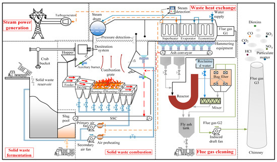
Figure 1.
MSWI System.
To enhance combustion efficiency, the furnace temperature is strictly maintained within the range of 850–1100 °C to ensure complete combustion. This not only improves the completeness of combustion but also effectively reduces the generation of unburned material. The achievement of high-efficiency combustion implies that a greater amount of harmful substances can be effectively converted rather than being released into the atmosphere as toxic gases, thereby reducing the quantity of emissions. For flue gas treatment, technologies such as neutralization reactions, adsorptive removal, and multi-stage dust removal are employed to eliminate NOX, sulfur dioxide (SO2), and particulate matter from the flue gas. To effectively reduce NOX emissions, low-NOX combustion technologies, such as staged combustion and optimized burner design, are adopted. These techniques suppress the formation of NOX by precisely controlling the temperature and oxygen distribution within the furnace.
2.2. Analysis of Factors Influencing Combustion Efficiency and NOX Emissions in the MSWI
To elucidate the intricate relationship between operational parameters and their dual effects on combustion efficiency and NOX emissions, Table 1 provides a concise summary of these influences, highlighting both the positive and negative aspects of each parameter.

Table 1.
Operational Parameters Affecting Combustion Efficiency and NOX Emissions.
In MSWI, primary air volume, secondary air volume, air pressure, and grate speed collectively regulate the combustion conditions within the furnace, significantly affecting both combustion efficiency and NOX emissions. The primary air supplies oxygen for initial combustion on the grate—an appropriate volume enhances efficiency, but excess air reduces furnace temperature and increases NOX. Secondary air promotes burnout and gas mixing in later stages, improving efficiency, though excessive amounts can elevate NOX formation, while insufficient air may result in incomplete combustion. Air pressure drives the airflow into the furnace; higher pressure increases flow velocity and efficiency, but overly high levels may cause excessive temperature rise and promote NOX production. Grate speed governs waste residence time: too low a speed leads to over-combustion, elevated temperatures, and higher NOX emissions, whereas too high a speed shortens combustion time, reduces efficiency, and raises unburned matter levels. These variables interact through multiple pathways, such as temperature, oxygen concentration, and airflow distribution, resulting in a dynamic, nonlinear coupling relationship between efficiency and NOX emissions, with a notable trade-off: high efficiency often accompanies high NOX emissions, while reducing NOX may compromise efficiency [7].
Additionally, frequent adjustments of grate speed are undesirable, as they can compromise combustion stability and efficiency, potentially resulting in incomplete combustion or equipment failure. Since grate speed determines the residence time of waste in the furnace and influences combustion uniformity [28], and is not suitable for frequent regulation, it is treated as an operational condition in this study.
Therefore, the control objective is to identify changing operational conditions based on grate speed and dynamically optimize the primary air volume, secondary air volume, and air pressure during the incineration process. This aims to maximize combustion efficiency while ensuring that NOX emissions remain within acceptable limits. Essentially, this constitutes a dynamic nonlinear multi-objective optimization problem [29].
3. Optimal Control Method for the MSWI Process Based on IWOA-RBF-IPOA
3.1. Definition of Optimal Control for the MSWI Process
Prior to detailing the proposed strategy, it is crucial to define what constitutes “optimal control” within the specific context of Municipal Solid Waste Incineration (MSWI). Unlike general combustion processes that may prioritize thermal efficiency or a single pollutant, optimal control in MSWI is a multi-faceted problem defined by the need to simultaneously satisfy technical, environmental, and operational constraints under highly variable conditions.
For the MSWI process, an optimal control method is defined as a strategy that dynamically manipulates the key operational variables—primary air flow , secondary air flow , and air pressure —to achieve a Pareto-optimal balance among the following core objectives:
- Maximize Combustion Efficiency : Ensure the complete destruction of waste and maximize energy recovery, which is intrinsically linked to maintaining a high CO2/CO ratio in the flue gas.
- Minimize Environmental Impact : Suppress the formation of regulated pollutants, most notably NOX, to levels strictly below the mandated emission limits.
- Ensure Operational Feasibility and Safety: Maintain all process variables within safe operating limits and, critically, ensure that CO emissions remain below the regulatory threshold ([CO] ≤ [CO]max) to prevent incomplete combustion and the potential formation of toxic by-products.
Furthermore, the controller must be inherently robust and adaptive to cope with the primary source of disturbance in MSWI: the unpredictable variation in waste composition, feed rate (grate speed, Ω), and consequent calorific value. Therefore, an optimal control method in this context is not one that finds a single, static setpoint, but one that continuously seeks the best possible compromise in a dynamically changing environment.
The hybrid strategy proposed in the following sections is designed explicitly to meet this MSWI-specific definition of optimal control.
3.2. Control Objectives
In the MSWI process, combustion efficiency is a key indicator for evaluating combustion quality. Generally, combustion efficiency can be characterized by the ratio of CO2 to CO concentrations in the flue gas. During complete combustion, CO2 is the primary product, while CO is a byproduct of incomplete combustion. Therefore, a higher CO2 concentration and a lower CO concentration indicate higher combustion efficiency. Based on this, combustion efficiency can be defined as:
In Equation (1), denotes the combustion efficiency, expressed as a percentage. A higher value indicates more complete combustion.
On the other hand, nitrogen oxide (NOX) emissions are an environmental indicator that requires strict control during the incineration process. Its concentration must comply with national emission standards and should be minimized as much as possible under given constraints. Therefore, the NOX emission concentration is treated as an objective function to be minimized.
However, the core challenge in MSWI optimization lies in the inherent trade-offs among the different objectives. The combustion parameters that are optimal for minimizing one pollutant are often suboptimal for another. This is because a fundamental competition exists between achieving high combustion efficiency which is intrinsically linked to low CO and high CO2 concentrations—and minimizing NOx emissions . The underlying mechanism for this trade-off is critical to understand:
High-efficiency, low-CO conditions necessitate high temperatures and sufficient oxygen to ensure complete combustion. Unfortunately, these very conditions are highly conducive to the thermal formation of NOx, leading to an increase in .
Conversely, low-NOx conditions are typically achieved through strategies like air staging or reduced combustion temperature, which can create oxygen-deficient or cooler zones. This undermines complete combustion, resulting in a significant increase in carbon monoxide (CO) emissions and a corresponding decrease in combustion efficiency .
Therefore, the optimization objective of maximizing while minimizing inherently defines a multi-objective problem that seeks a Pareto-optimal compromise. This compromise must consciously account for the behavior of CO emissions, which are directly embedded in the definition of . The goal of our approach is to intelligently navigate this three-way trade-off (efficiency-NOx-CO) to identify operating conditions that yield a practically acceptable and balanced performance across all key indicators.
Define the manipulated variables (MVs) as shown In Equation (2).
In Equation (2), , , represent the primary air flow, secondary air flow, and air pressure, respectively. The multi-objective optimization problem can then be formulated as simultaneously maximizing combustion efficiency and minimizing NOX emission concentration , and minimizing NOx emission concentration. This is mathematically described as follows:
The constraints include:
In Equation (4), and are the lower and upper limits for the primary air flow, respectively; and are the lower and upper limits for the secondary air flow, respectively; and are the lower and upper limits for the air pressure, respectively; and are the allowable ranges for the operating condition parameter (grate speed); is defined as the grate-speed operating index. This multi-objective optimization problem aims to find a set of MVs, such that, under all process constraints, the combustion efficiency is as high as possible and the NOX emission concentration is as low as possible.
3.3. Control Strategy
Based on the characteristic analysis of the MSWI process in Section 2.2, this study aims to address its distinctive nonlinear dynamic optimization problem under highly fluctuating operational conditions. Unlike combustion processes with stable fuel sources (e.g., natural gas or coal), MSWI is characterized by the heterogeneous nature and highly variable calorific value of municipal solid waste. This fuel heterogeneity leads to frequent and significant disturbances in the furnace, causing rapid changes in temperature and combustion gas composition. Consequently, the operational parameters require more frequent and adaptive adjustments to maintain stable and compliant combustion. The control objectives in MSWI are also uniquely complex, simultaneously prioritizing combustion efficiency (to ensure waste harmless treatment), energy recovery, and strict control of multiple pollutants (NOX, CO) to meet environmental regulations. The proposed hybrid optimal control strategy is specifically designed to address these MSWI-specific challenges.
Based on the characteristic analysis in Section 2.2, this study aims to address the nonlinear dynamic optimization problem under varying operational conditions. Given that the Pelican Optimization Algorithm (POA) exhibits strong global search capability and fast convergence speed, and has been successfully applied to multi-objective optimization of industrial gas leakage in reference [30], POA is selected to optimize the manipulated variables in this work. Since combustion efficiency is closely related to the concentrations of carbon monoxide (CO) and carbon dioxide (CO2), a combustion efficiency prediction model is necessary to proactively identify and mitigate potential disturbances, thereby providing reference and evaluation criteria for the POA-based optimization process. In view of the complex nonlinear relationship between CO, CO2, and combustion efficiency, an RBF neural network is adopted to develop the prediction model. RBF networks are widely used in such tasks due to their ability to approximate complex nonlinear mappings with high accuracy [31]. This model enables precise prediction of the concentrations of emissions such as CO, CO2, and NOX. During the combustion process, the generation of these emissions is influenced by multiple operational factors and varies with changing conditions. Therefore, dynamic optimization of key parameters determining model accuracy is essential, which inherently constitutes a nonlinear parameter optimization problem. Reference [32] has demonstrated the effectiveness of the WOA in handling industrial nonlinear parameter optimization. Building on this, an improved WOA version is proposed in this paper to better adapt to complex nonlinear optimization tasks and achieve optimal parameter identification.
Specificity of the MSWI Process and Control Objectives
The MSWI process exhibits several critical distinctions from conventional combustion processes, which directly inform the design of our control strategy:
Highly Variable Feedstock: The composition and calorific value of MSW change hourly and daily, leading to unpredictable fluctuations in the combustion state. This necessitates a control system capable of rapid adaptation, far beyond what is required for uniform fuels.
Stringent Multi-Pollutant Control: The control objective is not merely thermal efficiency. It is paramount to minimize emissions of nitrogen oxides (NOX), a major atmospheric pollutant, while simultaneously ensuring complete combustion to minimize carbon monoxide (CO), an indicator of incomplete combustion and dioxin precursor. This multi-objective, often conflicting, requirement is a hallmark of advanced MSWI control.
Coping with High Calorific Value: Modern MSW can have a high calorific value, which, if not properly managed, can lead to excessively high furnace temperatures that damage equipment and increase NOX formation. This requires precise control of air distribution and grate movement to manage the heat release rate and ensure sufficient residence time for complete combustion.
To clearly delineate the framework of our MSWI-focused model, the specific inputs and outputs are defined in Table 2.
Table 2.
MSWI-specific inputs and outputs of the proposed hybrid optimal control strategy.
Based on the above analysis, this paper proposes a hybrid optimal control strategy as shown in Figure 2, comprising three modules: a K-means and IWOA-based RBF prediction model for CO, CO2, and NOX, an IPOA-based air volume and pressure optimization setting module, and a combustion evaluation model. The inputs to the IWOA-RBF-based prediction model for CO, CO2, and NOX are the operating condition data (grate speed) , primary air flow , secondary air flow and air pressure . The combined IWOA-RBF method is used to determine the predicted values , , for CO, CO2, NOX, and the improved IWOA is employed to optimize the neuron width σ in the prediction model. The inputs to the IPOA-based air volume and pressure setting module are the target combustion efficiency, target nitrogen oxide emission concentration, and operating condition (grate speed). The IPOA is used to optimally set the primary air flow, secondary air flow, and air pressure to achieve the target combustion efficiency and nitrogen oxide emission concentration; the combustion evaluation model, based on CO, CO2, and NOX, assesses whether the combustion efficiency and emission concentrations meet the target values and feeds this information back to the IPOA to guide the next optimization process.
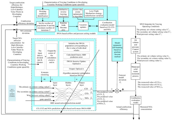
Figure 2.
Optimal control strategy of the MSWI process.
3.4. Control Algorithms
3.4.1. Prediction Models Based on IWOA-RBF for CO, CO2, NOX
In this study, an RBF neural network is selected to construct the emission prediction model for CO, CO2, and NOX. The RBF network exhibits local response characteristics and optimal approximation capabilities. The Gaussian functions in its hidden layer respond significantly only to inputs near their center points, which aligns well with the characteristics of combustion process variations, where different operational intervals exhibit distinct dynamic behaviors. Furthermore, the RBF network offers faster training speed, making it more suitable for engineering scenarios requiring online or rapid optimization [33].
RBF Network Structure
The prediction RBF model consists of an input layer, a hidden layer, and an output layer. The input layernodes, connected to the primary air flow , secondary air flow , air pressure , and operating condition (grate speed) Ω, respectively. The output layer includes three neurons, connected to the predicted values for CO, CO2, NOX: , , .
The output of the network can be described as [34]:
In Equation (5), Y is the vector of model output variables, is the input vector to the model, representing primary air flow, secondary air flow, air pressure, and operating condition, the output of the j-th neuron in the hidden layer uses a Gaussian RBF [35].
In Equation (6), is the center of the j-th RBF, determined by the K-means clustering method, which also determines the number of hidden layer nodes m; are determined by the Improved Whale Optimization Algorithm (IWOA); is the connection weight from the j-th neuron in the hidden layer to the output layer, determined by the gradient descent learning algorithm. The gradient descent algorithm defines the loss function as the mean square error as follows [36]:
In Equation (7), , , represent the measured values of CO, CO2, NOX, respectively. , , represent the predicted values of CO, CO2, NOX, respectively. is the learning rate. The parameters are updated iteratively according to Equation (9) along the negative gradient direction of the loss function with respect to achieving weight optimization.
Determination of Hidden Layer Node Number m and Centers C Using K-Means Clustering Algorithm
This paper introduces the K-means clustering algorithm to identify regions where the data distribution is most compact and dense. Its key advantage lies in the isotropic nature of Euclidean distance, which measures differences uniformly in all directions [37]. The specific implementation steps are as follows:
For each input data point, including primary air volume, secondary air volume, air pressure, and grate speed, the Euclidean distance to all cluster centers C = {C1, C2, …, Cₖ} is calculated using Equation (10).
In Equation (10), is the Euclidean distance between the i-th data point and the i-th cluster center. A smaller distance indicates a higher degree of similarity between that data point and the center of the corresponding cluster. represents the i-th data point (input vector). This vector constitutes a set containing the specific numerical values of multiple manipulated variables, such as primary air flow, secondary air flow, grate speed, and air pressure. represents the i-th cluster center (centroid). It is a vector with the same dimensionality as the data points, representing the average characteristics of all members belonging to a specific cluster. is the j-th feature value of the i-th data point. is the j-th feature value of the i-th cluster center.
Subsequently, for each data point, determine the minimum distance to all cluster centers using Equation (11):
In Equation (11), represents the minimum distance from a specific data point u to all cluster centers. d1(u), d2(u), …, dk(u): These denote the distances from the same data point u to the 1st, 2nd, …, k-th cluster centers, respectively (all these distances are calculated using Formula (9). Assign this point to the cluster whose center is nearest. After all points have been assigned, calculate the new center (mean) for each cluster according to Formula (12).
In Equation (12), is the new center point of the j-th cluster, and is the total number of operating condition points within this cluster.
During the iterative process of the algorithm, check whether the change between the old and new cluster centers is less than a preset threshold ɛ using Formula (13).
In Equation (13), is the newly calculated center point for the j-th cluster in the current iteration (calculated using Equation (12)). is the center point used for the j-th cluster in the previous iteration. If the change for all cluster centers is less than the threshold, terminate the iteration.
The pseudocode for the K-means clustering algorithm is presented in Algorithm 1.
| Algorithm 1: K-Means Clustering Pseudocode |
| 1: Begin K-Means algorithm 2: Input datasets V and number of clusters K 3: Determine maximum iterations T and convergence threshold ε 4: Randomly initialize cluster centers C = {c1, c2, …, cₖ} 5: For t = 1 : T: 6: Phase 1: Data point assignment 7: For i = 1 : n: 8: For j = 1 : K: 9: Calculate distance using Formula (10) 10: End 11: Determine minimum distance using Formula (11) 12: Assign input data to the nearest cluster center 13: End 14: Phase 2: Cluster center update 15: For j = 1 : K: 16: Calculate new center using Formula (12) 17: End 18: Check convergence condition using Formula (13) 19: If converged: 20: Break 21: Else: ) 23: End 24: End 25: Output clustering result C = {C1, C2, …, Cₖ} 26: End K-Means algorithm |
The number of clusters K determined by the K-means algorithm directly defines the number of hidden layer neurons m in the RBF neural network, and the cluster center points C determine the centers of each RBF in the hidden layer of the RBF neural network.
Determination of Neuron Widths Based on IWOA
In RBF neural network modeling, the neuron widths are core parameters, whose physical meaning reflects a “similarity sensitivity threshold” between input samples and the cluster centers. When the neuron width is too small, the effective range of the RBF narrows, making the model prone to overfitting and increasing its sensitivity to noise. Conversely, when the neuron width is excessively large, the output distinctions between neurons become blurred, leading to a loss of detailed features and consequently reducing the approximation accuracy. The value of the neuron width directly determines the model’s nonlinear mapping capability, which in turn affects its generalization ability and stability. Furthermore, the neuron width is closely related to the information transmission efficiency between the hidden layer and the output layer. Particularly in the MSWI process, the optimal value for the neuron width adjusts dynamically with changes in operating condition indicators such as grate speed, and exhibits a strongly nonlinear relationship with these conditions. Therefore, determining the optimal values for the neuron widths is essentially a nonlinear parameter identification problem influenced by operating conditions, significantly impacting the model’s performance.
This paper employs a WOA to optimize the neuronal width parameters of the RBF neural network. The WOA simulates the hunting behavior of humpback whales, achieving optimization through three phases: encircling prey, bubble-net attacking, and random search. The relationship between the optimization problem and whale behavior is summarized in Table 3. The optimization of neuronal widths in the RBF neural network is analogous to whales tracking prey in the ocean. In this mapping, the key parameters of the RBF network correspond to the position of prey, while the position of individual whales represents a set of potential parameter solutions. The behaviors of searching, encircling, and attacking prey in the algorithm correspond to the steps of broad exploration, local exploitation, and final determination of the optimal solution in the parameter optimization process. The individual position update mechanism in the WOA, as described by Equation (18), is particularly crucial for the prediction of CO, CO2, and NOX emissions. This mechanism helps prevent the model from converging to local optima, thereby enhancing prediction accuracy and generalization capability.
Table 3.
Correspondence between the WOA and the Optimization Problem for Parameters .
- (1)
- Limitations of the Standard WOA for the Optimization Problem
The standard WOA, by simulating the predatory behavior of humpback whales, embodies a unique symmetry mechanism. Its core lies in the spiral encircling prey strategy, as shown In Equation (14).
In Equation (14), represents the state at the next time step, is the position vector of the current best search agent, is the position vector of the current search agent, represents the distance between the current individual and the best solution, is a constant defining the logarithmic spiral shape (usually set to 1), is a random number in [−1, 1].
The parameters controlled mechanism is achieved through the following equations:
In Equations (15) and (16), and are random numbers within [0, 1]. The coefficient vectors and are used to control the search behavior of the whale individuals.
The algorithm balances the exploration and exploitation stages through parameters, and its linearly decreasing mechanism is shown in Equation (17).
In Equation (17), t is the current iteration number, and is the maximum number of iterations. The random fluctuation of parameter A creates dynamic symmetry-promoting global exploration when (large-scale symmetric search of the space), and shifting to local exploitation when (fine symmetric search around the current best solution).
- (2)
- IWOA Improvement Strategies for Combustion Condition Optimization
Considering the characteristics of the MSWI process, four improvements are made to the standard WOA to enhance its optimization performance.
- (i)
- Nonlinear Convergence Factor Adjustment Strategy
This paper adopts a nonlinear convergence factor adjustment strategy. In the early stages of iteration, it maintains a strong global exploration capability, facilitating the identification of promising regions within the complex parameter space. During later iterations, it accelerates convergence and focuses on local exploitation, thereby effectively balancing exploration and exploitation while avoiding the rigidity associated with traditional linearly decreasing factors [38].
First, define the nonlinear convergence factor, as shown in Equation (18):
In Equation (18), is an adjustment exponent. This strategy maintains a larger value in the early optimization phase, enhancing global exploration capability; In the later optimization phase, it rapidly decreases the value, strengthening local exploitation precision, effectively maintaining a dynamic balance between exploration and exploitation phases.
- (ii)
- Adaptive Spiral Weight Mechanism
To enhance the adaptability of the spiral search process, an adaptive weight factor is introduced. This mechanism dynamically adjusts the step size of the spiral search, granting the algorithm stronger global exploration capability initially, and gradually transitioning to fine local exploitation as the search progresses. This simulates the whale’s hunting process from long-distance encircling to close-range precise attack, significantly improving the algorithm’s convergence accuracy and stability in complex flue gas prediction problems [39].
The improved spiral update Equation is:
In Equation (19), , endow the algorithm with strong global exploration ability in the initial iterations, gradually transitioning to local fine search as iterations proceed.
- (iii)
- Levy Flight Disturbance Strategy
To prevent the algorithm from falling into local optima, the Levy flight mechanism is introduced. The Levy flight, characterized by occasional long-distance jumps, can effectively help the population escape local optima traps and enhance global search capability when incorporated into the algorithm. This is crucial for multimodal, high-dimensional parameter optimization problems in flue gas concentration prediction, significantly increasing the probability of finding the global optimal solution.
In Equation (21), represents the Levy flight, and is a parameter controlling the shape of the distribution. A Levy flight is a random process characterized by a step length distribution with a high probability of long-distance jumps. is a step size parameter controlling the magnitude of the update.
- (iv)
- Differential Mutation Operation
To address the issue of maintaining population diversity, differential mutation is applied to the worst 20% of individuals. Mutating poorer individuals is equivalent to injecting new genetic information into the population, greatly enhancing its diversity. This effectively prevents the algorithm from falling into local optima due to premature homogenization of the population, ensuring the algorithm remains vigorous even in the later stages of optimization [40].
In Equation (22), F is the mutation factor, and are randomly selected individuals. This operation effectively improves population quality and avoids premature convergence. The pseudocode summarizing the IWOA-based optimization algorithm for neuron width parameters is presented in Algorithm 2. The corresponding flowchart is depicted in Figure 3.
| Algorithm 2: IWOA Pseudocode |
| 1: procedure IWOA_RBF_TUNING 2: Define inputs: Training data {H, Q}, RBF centers C, Population size N, Max iterations T, p_levy 3: Define output: Optimal width parameters σ= {σ1, σ2, …, σm} 4: Initialize whale population Hi(0)= {σ1, σ2, …, σm} 5: Calculate fitness f(Hi(0)) for each individual using Formula (23) 6: Determine current best individual H* 7: for t = 1 : T : 8: Update convergence factor a using Formula (18) 9: Update spiral weight ω using Formula (19) 10: Assuming (15) refers to the formulas for A and E 11: for Hi : 12: if p < 0.5 : 13: if |A| < 1 : 14: Perform encircling prey using Formula (16) 15: else 16: Perform random search using Formula (16) 17: end if 18: else 19: Perform spiral update using Formula (20) 20: end if 21: Apply Levy flight disturbance using Formula (21) with probability p_levy 22: Calculate new fitness f(Hi(t)) using Formula (23) 23: end for 24: Perform differential mutation on the worst 20% individuals using Formula (22) 25: Update the best individual H* 26: end for 27: return σ* = H* 28: end |
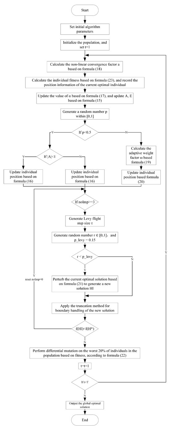
Figure 3.
Flowchart of the IWOA for the Optimization Process.
Based on this, IWOA is applied to optimize the RBF neural network width parameters , aiming to minimize the mean square error of multi-component flue gas (CO, CO2, NOX) prediction. The error function is defined as:
In Equation (23), is the vector of width parameters to be optimized, N is the number of training samples, and represent and the actual and predicted values, respectively, of the flue gas component (CO, CO2, NOX) for the i sample of the k gas type, where k = 1, 2, 3 represents CO, CO2, NOX, respectively.
During the optimization process, each whale individual corresponds to a set of width parameter configurations, and its fitness is evaluated based on the performance of the corresponding RBF network in multi-component flue gas prediction. By effectively balancing exploration and exploitation, IWOA can efficiently search for the optimal parameter configuration in the parameter space, thereby enhancing the RBF neural network’s ability to model flue gas emission characteristics under different combustion conditions.
3.4.2. IPOA-Based Optimization Method for Air Volume and Pressure
This paper employs the POA to optimize the air volume and pressure manipulated variables. POA is a novel metaheuristic algorithm proposed in 2022 [31]. Its basic principle simulates the collective behavior of pelicans during hunting, including two phases: exploration (moving towards prey) and exploitation (wing flapping and feeding). Compared to traditional optimization algorithms, POA has advantages such as fewer parameters, simple implementation, and high search efficiency, making it suitable for solving engineering optimization problems. However, the traditional POA still has some shortcomings when handling complex multimodal optimization problems. This paper improves it specifically for the MSWI process.
Limitations of the Traditional POA
The traditional POA mainly includes the following three core mathematical Equations:
(1) Population initialization Equation
In Equation (24), represents the position of the i-th individual in the j-th dimension, and are the lower and upper bounds of the j-th dimension variable, respectively, rand is a random number within [0, 1], N is the population size, and m is the problem dimension.
(2) Position Update Formula for Exploration Phase
In Equation (25), is the new position after the exploration phase, is the position of the prey, and are the fitness values of the prey and the current individual, respectively, and I is a random integer, rand is a random number within [0, 1].
(3) Position Update Formula for Exploitation Phase
In Equation (26), is the new position after the exploitation phase, R is a constant, t is the current iteration number, and T is the maximum number of iterations.
The limitations of the traditional POA are primarily reflected in three aspects: its overly simplistic initialization strategy leads to insufficient population diversity; the excessively strong randomness in the exploration phase results in low search efficiency; and the local search in the exploitation phase employs a linearly decreasing mechanism, which struggles to balance global exploration and local exploitation, making the algorithm prone to premature convergence.
Improvement Strategies for POA
(1) Refraction Opposition-Based Learning Initialization Strategy
A refraction opposition-based learning mechanism is adopted to enhance population diversity. In the optimization of air volume and pressure, the quality of the initial population directly influences the optimization efficiency. Given the complex and variable operational conditions of MSWI, simple random initialization may cause the population to distribute in suboptimal regions. The refraction opposition-based learning mechanism generates more uniform and diverse initial solutions, ensuring that the algorithm comprehensively scans the solution space formed by the primary air volume, secondary air volume, and air pressure from the outset. This significantly improves the probability of finding globally optimal settings [41].
In Equation (27), k is the refraction coefficient, used to control the strength of opposition-based learning, is the original opposite solution. This strategy can generate an initial population with a more uniform distribution.
(2) Strategy Integrating Sine Cosine Algorithm (SCA)
The air volume and pressure system represents a complex nonlinear system characterized by strong coupling relationships between input variables. The sine and cosine oscillatory properties of the SCA provide an adaptive rhythm for population updates: when oscillations are large, they facilitate global exploration to discover new combinations of air volume and pressure. When oscillations are small, they enable local exploitation to finely adjust current settings [42]. This dynamic adjustment mechanism allows the IPOA to better adapt to the nonlinear characteristics of the combustion system.
Introducing the fluctuation characteristics of the Sine Cosine Algorithm (SCA).
In Equations (28) and (29), q is a constant, is a random number within determining the movement direction, is a random number within [0, 2] controlling the global search ability, is a random number within [0, 1] used to choose between sine or cosine operation, and is the position of the current global best solution in the j-th dimension. Calculation results show that as iteration time increases, the influence of each particle on subsequent particles is nonlinear. When or (or conceptually when the coefficient multiplied is large), it is conducive to global search for the next generation; When or (or conceptually when the coefficient multiplied is small), it is conducive to local search for the next generation.
(3) Levy Flight Perturbation Strategy
The combustion process is susceptible to disturbances such as fluctuations in waste calorific value, and the objective function (fitness) may contain multiple local optima. The long-distance jumping characteristics of Levy flight allow the algorithm to suddenly escape from currently apparent optima (which are actually local optima) in air volume and pressure settings, continuing to search for better solutions throughout the solution space, thereby enhancing the algorithm’s robustness under complex operating conditions [43]. To prevent the algorithm from becoming trapped in local optima, a Levy flight mechanism is introduced.
In Equation (30), is the Levy flight, is a parameter controlling the shape of the distribution. The Levy flight is a random process characterized by a step length distribution with a high probability of long-distance jumps. is the step size parameter, controlling the magnitude of the update.
(4) t-Distribution Mutation Based on Iteration Count t
The shape of the t-distribution varies with the degrees of freedom. In the early stages, it resembles a Cauchy distribution, favoring global exploration; In later stages, it approximates a Gaussian distribution, favoring local exploitation. This characteristic perfectly aligns with the requirements of air volume and pressure optimization: the initial phase requires broad exploration of various air ratio configurations, while the latter phase demands fine-tuning to achieve stable and precise optimal settings. This strategy adaptively adjusts the mutation intensity, achieving an automatic balance between exploration and exploitation [44].
In Equation (31), is the current global best solution, are random individuals from the population represents a random variable following the h-distribution with the current optimization count t as its degrees of freedom. This strategy gives the algorithm strong global exploration capability in the early stages, gradually shifting to local fine search in the later stages.
3.5. Implementation Steps of the Air Volume and Pressure Optimization Control Algorithm
The IPOA simulates the natural hunting behavior of pelicans. It begins by randomly generating candidate values for the primary air volume and pressure, as well as the secondary air volume and pressure. The process consists of two phases: the first is movement towards the prey (exploration phase), where the population continuously scans the search space to locate potential air volume and pressure settings, and subsequently moves toward these identified settings; the second phase is wing-vibration flight (feeding phase), which involves continuous iterations to find the optimal feeding location. Throughout the iterations, a fitness function is used to evaluate the performance of each candidate solution. After each optimization step, the values are input into the prediction models for CO, CO2, NOX to compute updated combustion efficiency and NOX emission levels. The fitness function is then updated accordingly. In the context of optimizing air volume and pressure settings for MSWI, the dual objectives of achieving maximum combustion efficiency and minimizing pollutant emissions necessitate multiple optimization cycles and enhanced search capabilities to progressively approach the ideal air volume and pressure settings.
This paper employs the IPOA to optimize the settings for air volume and pressure, corresponding to the manipulated variables defined in Equation (2). The fitness function for this optimization is:
In Equation (32), is the current nitrogen oxide concentration, is the maximum NOX concentration, is the combustion efficiency, and is the maximum combustion efficiency. The term represents the normalized combustion efficiency; a larger value indicates higher efficiency, which is the target we want to maximize. The term represents the normalized NOX concentration; a larger value indicates more severe pollution, which is the target we want to minimize.
Therefore, the fitness function is designed as Equation (32). In this form, the multi-objective optimization problem (maximizing efficiency and minimizing NOX emissions) is successfully transformed into a single-objective maximization problem.
When the value calculated by (32) reaches its maximum, it indicates that the system has simultaneously achieved high combustion efficiency and low NOX emissions under the current conditions, finding the optimal balance between these two objectives. This function ingeniously combines two indicators that may have different dimensions and orders of magnitude through a normalization process, thereby guiding the IPOA to search for the ultimate goal of ‘high efficiency and low pollution’.
The correspondence relationship between IPOA and the optimization of the air volume and pressure is shown as follows (Table 4).
Table 4.
Correspondence relationship between IPOA and the optimization question.
Specifically, the target combustion efficiency, target NOX emission concentration, and operational data (grate speed) are first input into the air volume and pressure setting module. An initial air volume and pressure value is set and fed into the prediction model, which outputs predicted values for CO, CO2, and NOX. These predicted values are then sent to the evaluation model for assessing combustion efficiency and NOX emissions. Based on the evaluation results—specifically the deviations between the predicted and target values of combustion efficiency and NOX concentration-the next optimization direction is determined to update the air volume and pressure settings, completing one iteration cycle. This process repeats iteratively: the updated air volume and pressure settings are again fed into the prediction model, and the newly predicted values , , are evaluated by the evaluation model. The cycle continues until the output evaluation indicators approach the target values. At this point, the optimal primary air volume , secondary air volume , and air pressure are output as final results and subsequently sent to the air volume and pressure control system for implementation. This ultimately maintains both combustion efficiency and NOX emissions within the required process limits. Based on the above research, this paper utilizes the IPOA to optimize the air volume and pressure settings. The flowchart is shown in Figure 4.
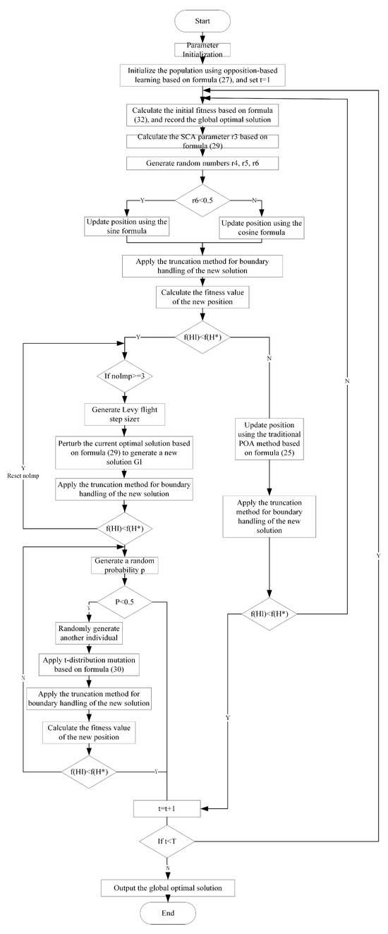
Figure 4.
Flowchart of the IPOA Optimization Process.
The specific implementation procedure is as follows:
Step 1: When the incineration system reaches stable operation, input the target combustion efficiency, target NOX emission concentration, and operational conditions (grate speed) into the IPOA-based air volume and pressure setting module to generate initial air volume and pressure settings.
Step 2: Feed the initial air volume and pressure settings into the prediction model described in Chapter 3 of this paper. The prediction model then outputs the predicted values for CO, CO2, and NOX , , .
Step 3: Send the predicted values , , to the combustion evaluation model to assess combustion efficiency and nitrogen oxide emission concentration. If the assessment is close to the target values, output the air volume and pressure setting.
Step 4: If there is a significant deviation, repeat steps 1, 2, and 3 until the values are close to the targets.
Step 5: Send the finally generated air volume and pressure setting , , to the air volume and pressure control system for implementation.
4. Experimental Design and Result Analysis
4.1. Experiment of the K-Means and IWOA-RBF-Based Prediction Models for CO, CO2, NOX
4.1.1. Data Description
The experimental platform used in this study operated on a Windows 11 system, with model training and prediction carried out using MATLAB R2021a. The data employed were sourced from the Distributed Control System (DCS) of a forward-moving grate incinerator at a MSWI plant in Beijing, China. This dataset consists of 12,000 measurements collected at 1-s intervals, which is divided into four subsets, each containing 3000 data points. For each subset, 2000 data points were used as the training set for model development, 500 points as the test set for prediction evaluation, and 500 points as the validation set. The parameter configurations for IWOA are presented in Table 5.
Table 5.
The parameter configuration of IWOA.
4.1.2. Experimental Results and Analysis
This study employs an IWOA-RBF for experimentation. The number of hidden layer nodes in the RBF neural network was determined to be 8 based on the K-means clustering algorithm, as presented in Table 6.
Table 6.
Cluster Result Table.
The optimization and identification of neuronal widths in the RBF neural network using the IWOA approach yielded the results shown in Table 7. These results demonstrate that the IWOA adaptively assigns optimal widths to each neuron that match the statistical characteristics of their respective data clusters, laying a solid foundation for constructing a high-performance prediction model.
Table 7.
Neuron Width Result Table.
This paper compares the prediction deviations of IWOA-RBF, WOA-RBF, and GWO-RBF models. The experiment aims to evaluate the prediction capabilities of different models in optimizing air volume and pressure for MSWI by analyzing the prediction deviations of the three optimization algorithms. The Root Mean Square Error (RMSE) and Mean Absolute Error (MAE) were employed to quantify the discrepancies between the predicted values of different optimization algorithms and the actual values, as shown in the following formulas:
In Equations (33) and (34), is the true value of CO, CO2, and NOX, is the corresponding predicted value. The results are presented in Table 8, Table 9, Table 10, Table 11, Table 12 and Table 13, which, respectively, show the comparison of RMSE and MAE for CO, CO2, and NOX emission concentrations using different optimization algorithms. As can be seen from the tables, the IWOA-RBF model achieved a reduction in RMSE for CO, CO2, and NOX emission concentrations compared to the WOA-RBF model, in terms of MAE and RMSE. This indicates that IWOA’s optimization capability surpasses that of WOA and GWO, enabling more precise optimization of RBF model parameters and thereby reducing the overall prediction error across multiple indicators.
Table 8.
Comparison of the MAE of the CO emission concentration.
Table 9.
Comparison of the MAE of the CO2 emission concentration.
Table 10.
Comparison of the MAE of the NOX emission concentration.
Table 11.
Comparison of the RMSE of the CO emission concentration.
Table 12.
Comparison of the RMSE of the CO2 emission concentration.
Table 13.
Comparison of the RMSE of the NOX emission concentration.
Figure 5, Figure 6 and Figure 7 display comparison charts of prediction deviations for CO, CO2, and NOX emission concentrations based on different datasets. From the figures, it can be observed that the predicted values of the IWOA-RBF model are closer to the actual values, with errors remaining within acceptable limits.
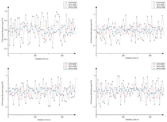
Figure 5.
Comparison chart of CO emission concentration based on datasets 1–4.
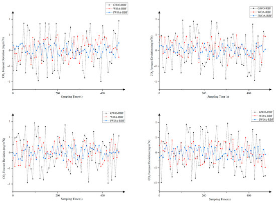
Figure 6.
Comparison chart of CO2 emission concentration based on datasets 1–4.
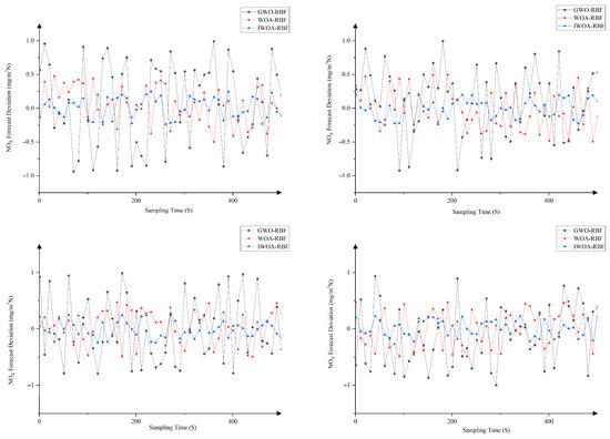
Figure 7.
Comparison chart of NOX emission concentration based on datasets 1–4.
From the above experimental results, it can be observed that the error fluctuation range of IWOA-RBF is reduced compared to WOA-RBF and GWO-RBF models. This indicates that the prediction deviation of IWOA-RBF remains more stable and is less susceptible to significant fluctuations caused by operational disturbances, demonstrating its superior generalization capability and disturbance resistance compared to the other models.
The IWOA-RBF model demonstrates significantly reduced errors across all three emission indicators (CO, CO2, and NOX). This indicates the model’s capability to simultaneously adapt to the nonlinear coupling relationships, validating its ability to capture the characteristics of multi-indicator coupling.
Figure 8 presents the normalized autocorrelation functions of the deviations between predicted and measured values for CO, CO2, and NOX based on datasets 1–4. As shown in the figures, the autocorrelation coefficients of the deviation sequences between predicted and measured values predominantly fall within the 95% confidence interval, indicating that the residual sequence can be considered white noise. This further substantiates the effectiveness of the prediction methodology proposed in this study.
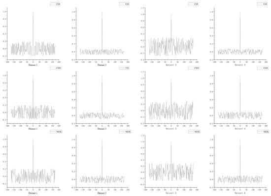
Figure 8.
The autocorrelation distribution results of CO, CO2, and NOX in Datasets 1–4.
4.2. Experiment of the Optimal Control
To rigorously validate the effectiveness and practical feasibility of the proposed hybrid optimal control method, an experimental scheme with a control group was designed. The experiment is structured in two stages: the first investigates the ability of the IPOA to escape local optima, while the second assesses the control performance of the system under diverse operational conditions.
4.2.1. Data Description
The data used for the validation experiments of the IPOA-based optimal control method is still sourced from the DCS of a forward-moving grate incinerator at a MSWI plant in Beijing, China. A total of 10,000 sets of measured data were collected, with a sampling interval of 1 s. Of these, 7000 sets were used as the training set, 1000 sets as the test set, and 2000 sets as the validation set. The parameter configuration for the IPOA is referenced in Table 14.
Table 14.
The parameter configuration for the IPOA.
4.2.2. Experimental Results and Analysis
(1) Comparison of IPOA and POA in Optimizing Airflow and Pressure Control
This experiment evaluates the capability of IPOA and POA to avoid local optima during the optimization of airflow and pressure control. Figure 9 illustrates the optimization process, with the horizontal axis representing the number of iterations and the vertical axis denoting the corresponding airflow or pressure values.
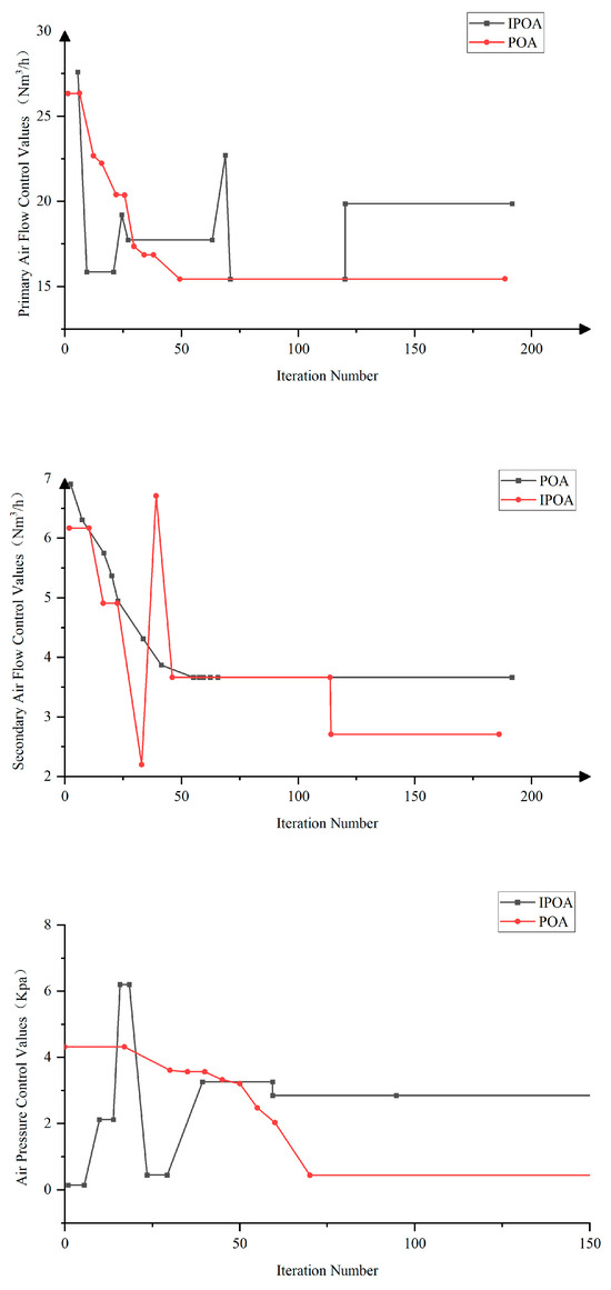
Figure 9.
Comparison of the optimization processes between IPOA and POA.
In the primary airflow optimization process, POA converged rapidly in the early iterations, with the fitness value entering the optimal range within the first ten generations. However, its search trajectory was relatively smooth, lacking global escape capability and making it susceptible to entrapment in local optima. By contrast, IPOA exhibited moderate fluctuations in the later stages, reflecting its stronger global search ability. Although the final fitness value obtained by IPOA was slightly higher than that of POA, it successfully escaped local minima, indicating its suitability for complex search spaces with multiple local optima.
In the secondary airflow optimization process, similar fluctuations were observed. IPOA expanded its search range, with the control values oscillating between 30 Nm3/h and 50 Nm3/h in the early stages. The algorithm continuously adjusted its search trajectory to identify an optimal solution that satisfied multiple objectives. In contrast, POA quickly stabilized the secondary airflow control value but became trapped in a local optimum due to its static search range.
In the airflow pressure optimization process, IPOA again demonstrated superior performance. During the initial iterations, the wind pressure control values fluctuated between 0.21 kN/m2 and 6.32 kN/m2. After several iterations, the values gradually stabilized, ultimately converging to approximately 3 kN/m2. This indicates that IPOA effectively expanded the search range, rapidly adapted to changes in target setpoints, and successfully escaped local optima. Conversely, POA exhibited a static search range and failed to overcome local entrapment.
In summary, the optimization results for both airflow and pressure in municipal solid waste incineration (MSWI) systems consistently demonstrate the superiority of IPOA over POA. Unlike POA, which converges rapidly but is prone to entrapment in local optima, IPOA effectively expands the search range, exhibits strong global exploration capability, and adapts more rapidly to dynamic operating conditions. This flexibility enables more robust and responsive adjustments to airflow and pressure control, ensuring stable system performance under fluctuating combustion environments. The ability of IPOA to balance exploration and exploitation is particularly critical for optimization problems characterized by nonlinear dynamics and frequent disturbances, as typically observed in waste incineration processes.
(2) Comparison of Combustion Efficiency and NOX Emissions Control Performance
To evaluate the control performance of the proposed method under dynamic operating conditions, with combustion efficiency and NOX emission concentration as control objectives, IPOA was compared with the existing control strategy implemented at a Beijing MSWI plant. The results under different operating conditions are presented in Figure 10 and Figure 11, while the four operating conditions, determined by grate speed, are summarized in Table 15.
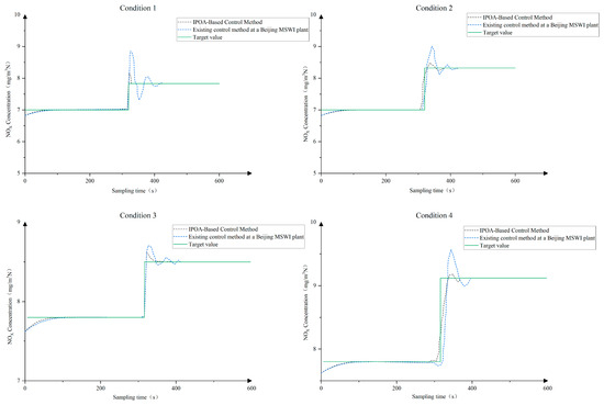
Figure 10.
Comparison of NOX emissions control performance based on condition 1–4.
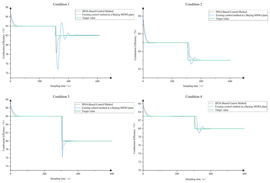
Figure 11.
Comparison of Combustion efficiency control performance based on condition 1–4.
Table 15.
The four operating conditions determined by the grate speed.
In the initial phase (approximately 100 s), the proposed method maintained combustion efficiency in the range of 83–86%, with a static deviation of about 0.3%. Meanwhile, the NOx emission concentration was controlled within 7–9%, with a static deviation of roughly 0.2%, indicating strong setpoint-tracking capability and operational stability.
When the operating conditions changed around 300 s, including variations in grate speed and target setpoints, the IPOA method promptly detected the disturbances and re-optimized the primary airflow, secondary airflow, and pressure control settings. This enabled the system to rapidly reach a new steady state. In contrast, the control method currently implemented at the plant, although responding quickly, exhibited pronounced overshoot, slower adjustments, and larger steady-state deviations.
Overall, the experimental results under four operating conditions demonstrate that the IPOA-based hybrid optimization method proposed in this study consistently outperforms the comparison methods in terms of control accuracy, response speed, and disturbance rejection.
5. Conclusions
This study proposes an optimal control method to enhance combustion efficiency and reduce nitrogen oxide (NOX) emissions in the MSWI process. By developing Radial Basis Function (RBF) neural network prediction models for CO, CO2, and NOX, and integrating the Improved Pelican Optimization Algorithm (IPOA), an optimized control strategy for air volume and pressure was established. Experimental results demonstrated that the proposed method not only improves combustion efficiency but also effectively reduces NOX emissions. Crucially, this enhancement in combustion efficiency directly translates into a positive energy effect. By minimizing incomplete combustion (reflected by low CO) and optimizing the air-fuel ratio, the method increases the net energy recovery from waste, thereby improving the overall energy efficiency of the incineration system and strengthening its role as a reliable waste-to-energy facility. Moreover, under varying operational conditions, IPOA adaptively adjusted airflow and pressure, ensuring system adaptability and maintaining both combustion efficiency and NOX concentrations within the target range.
Despite these promising results, several limitations remain. First, the scalability of the method requires further validation across different incineration plants and waste types. Second, the integration of RBF neural networks and IPOA introduces considerable computational complexity, necessitating future research to balance computational efficiency with control performance. Third, while this study primarily focuses on NOX emissions, future work could extend the approach to other pollutants, such as dioxins and particulate matter. Finally, the long-term stability of the method—particularly under equipment aging or varying waste composition—needs to be further examined.
In conclusion, the proposed IPOA-based control method provides a promising pathway for improving combustion efficiency and reducing pollutant emissions in MSWI systems. Nevertheless, continued refinement and validation are essential to enhance its robustness and ensure broader real-world applicability.
Author Contributions
Methodology, J.P. and P.D.; Software, P.D.; Validation, P.D.; Investigation, P.D.; Resources, J.T.; Writing—original draft, P.D.; Writing—review and editing, J.T.; Supervision, J.P. All authors have read and agreed to the published version of the manuscript.
Funding
This research received no external funding.
Data Availability Statement
The original contributions presented in this study are included in the article. Further inquiries can be directed to the corresponding author.
Conflicts of Interest
The authors declare no conflicts of interest.
Abbreviations
The following abbreviations are used in this manuscript:
| U | Input vector of the neural network |
| Primary air flow | |
| Secondary air flow | |
| Air pressure | |
| σ | Neuron width |
| the predicted values for CO | |
| the predicted values for CO2 | |
| the predicted values for NOX | |
| Primary air flow setting | |
| Secondary air flow setting | |
| Air pressure setting | |
| The lower limits for the primary air flow | |
| The upper limits for the primary air flow | |
| The lower limits for the secondary air flow | |
| The upper limits for the secondary air flow | |
| The lower limits for the air pressure | |
| The upper limits for the air pressure | |
| The lower limits for the operating condition parameter | |
| The upper limits for the operating condition parameter | |
| The combustion efficiency | |
| NOX emission concentration | |
| Y | The output of the network |
| Gaussian RBF | |
| The gradient descent algorithm | |
| The measured CO values | |
| The measured CO2 values | |
| The measured NOX values | |
| The Euclidean distance | |
| The i-th data point | |
| The i-th cluster center | |
| The j-th feature value | |
| The j-th feature value | |
| The minimum distance | |
| The new center point of the j-th cluster | |
| The center point used for the j-th cluster | |
| Convergence threshold | |
| The state at the next time step | |
| The position vector of the current best search agent | |
| The distance between the current individual and the best solution | |
| A constant | |
| A random number | |
| Random numbers | |
| Random numbers | |
| T | The maximum number of iterations |
| t | The current iteration number |
| a | The nonlinear convergence factor |
| Levy flight | |
| Parameter controlling | |
| A step size parameter controlling the magnitude of the update | |
| Randomly selected individuals | |
| Randomly selected individuals | |
| Q | Training data |
| N | Population size |
| The position of the i-th individual in the j-th dimension | |
| The lower bounds of the j-th dimension variable | |
| The upper bounds of the j-th dimension variable | |
| The new position after the exploration phase | |
| The position of the prey | |
| The fitness values of the prey | |
| The current individual | |
| The new position after the exploitation phase | |
| C | Center of the RBF |
| m | Number of hidden layer nodes |
| An adjustment exponent | |
| ωj | Connection weight from j-th hidden neuron to output |
| K | Number of candidate clusters |
| Z | Sample data |
| α | Adaptive parameter |
| β | Learning rate |
| A | Coefficient matrix in the whale algorithm formula |
| E | Coefficient matrix in the whale algorithm formula |
| p | Random number (typically in [0, 1])/Probability |
| R | A constant |
| The original opposite solution | |
| A random number | |
| A random number | |
| A random number | |
| q | A constant |
| The state at the next time step | |
| The current global best solution | |
| Random individuals from the population |
References
- Qiao, J.-F.; Guo, Z.-H.; Tang, J. Dioxin emission concentration measurement approaches for municipal solid wastes incineration process: A survey. Acta Autom. Sin. 2020, 46, 1063–1089. [Google Scholar] [CrossRef]
- dos Santos, I.F.S.; Mensah, J.H.R.; Gonçalves, A.T.T.; Barros, R.M. Incineration of municipal solid waste in Brazil: An analysis of the economically viable energy potential. Renew. Energy 2020, 149, 1386–1394. [Google Scholar] [CrossRef]
- Li, H.J.; Tan, D. Dynamic control of pollution of municipal solid waste incineration. Kybernetes 2025, 54, 727–748. [Google Scholar] [CrossRef]
- Margallo, M.; Taddei, M.B.M.; Hernández-Pellón, A.; Aldaco, R.; Irabien, Á. Environmental sustainability assessment of the management of municipal solid waste incineration residues: A review of the current situation. Clean Technol. Environ. Policy 2015, 17, 1333–1353. [Google Scholar] [CrossRef]
- Sun, J.; Meng, X.; Qiao, J. Data-driven optimal control for municipal solid waste incineration process. IEEE Trans. Ind. Inform. 2023, 19, 11444–11454. [Google Scholar] [CrossRef]
- Bose, D.; Ghanta, K.C.; Hens, A. CFD-based investigation of NOx removal from industrial waste gas by selective catalytic reduction (SCR) and selective non-catalytic reduction (SNCR) process using NH3. Int. J. Chem. React. Eng. 2025, 23, 701–713. [Google Scholar] [CrossRef]
- Wang, T.; Tang, J.; Xia, H.; Yang, C.; Yu, W.; Qiao, J. Data-driven multi-objective intelligent optimal control of municipal solid waste incineration process. Eng. Appl. Artif. Intell. 2024, 137, 109157. [Google Scholar] [CrossRef]
- Beylot, A.; Hochar, A.; Michel, P.; Descat, M.; Ménard, Y.; Villeneuve, J. Municipal solid waste incineration in France: An overview of air pollution control techniques, emissions, and energy efficiency. J. Ind. Ecol. 2018, 22, 1016–1026. [Google Scholar] [CrossRef]
- Nguyen, T.D.; Kawai, K.; Nakakubo, T. Drivers and constraints of waste-to-energy incineration for sustainable municipal solid waste management in developing countries. J. Mater. Cycles Waste Manag. 2021, 23, 1688–1697. [Google Scholar] [CrossRef]
- Chen, X.; Li, J.; Liu, Q.; Luo, H.; Li, B.; Cheng, J.; Huang, Y. Emission characteristics and impact factors of air pollutants from municipal solid waste incineration in Shanghai, China. J. Environ. Manag. 2022, 310, 114732. [Google Scholar] [CrossRef]
- Khan, S.; Anjum, R.; Raza, S.T.; Bazai, N.A.; Ihtisham, M. Technologies for municipal solid waste management: Current status, challenges, and future perspectives. Chemosphere 2022, 288, 132403. [Google Scholar] [CrossRef] [PubMed]
- Lu, J.-W.; Zhang, S.; Hai, J.; Lei, M. Status and perspectives of municipal solid waste incineration in China: A comparison with developed regions. Waste Manag. 2017, 69, 170–186. [Google Scholar] [CrossRef]
- Qiao, J.-F.; Meng, X.; Tang, Y.-T. Perspectives on Intelligent Optimized Control of Municipal Solid Waste Incineration Process under Dual Carbon Target. Bull. Natl. Nat. Sci. Found. China 2024, 38, 593–602. [Google Scholar] [CrossRef]
- Tang, J.; Tian, H.; Wang, T. A review of model predictive control for the municipal solid waste incineration process. Sustainability 2024, 16, 7650. [Google Scholar] [CrossRef]
- Hu, Q.-X.; Long, J.-S.; Wang, S.-K.; He, J.-J.; Bai, L.; Du, H.-L.; Huang, Q.-X. A novel time-span input neural network for accurate municipal solid waste incineration boiler steam temperature prediction. J. Zhejiang Univ. A 2021, 22, 777–791. [Google Scholar] [CrossRef]
- Yan, A.; Wang, R.; Guo, J.; Tang, J. A knowledge transfer online stochastic configuration network-based prediction model for furnace temperature in a municipal solid waste incineration process. Expert Syst. Appl. 2024, 243, 122733. [Google Scholar] [CrossRef]
- Bunsan, S.; Chen, W.-Y.; Chen, H.-W.; Chuang, Y.H.; Grisdanurak, N. Modeling the dioxin emission of a municipal solid waste incinerator using neural networks. Chemosphere 2013, 92, 258–264. [Google Scholar] [CrossRef] [PubMed]
- Zhou, H.; Zhao, H.; Zhang, Y. Nonlinear system modeling using self-organizing fuzzy neural networks for industrial applications. Appl. Intell. 2020, 50, 1657–1672. [Google Scholar] [CrossRef]
- Pian, J.; Liu, J.; Tang, J.; Hou, J. Intelligent Control of the Main Steam Flow Rate for the Municipal Solid Waste Incineration Process. Sustainability 2025, 17, 6036. [Google Scholar] [CrossRef]
- Tao, J.; Li, Z.; Chen, C.; Liang, R.; Wu, S.; Lin, F.; Cheng, Z.; Yan, B.; Chen, G. Intelligent technologies powering clean incineration of municipal solid waste: A system review. Sci. Total. Environ. 2024, 935, 173082. [Google Scholar] [CrossRef]
- Wen, C.; Lin, X.; Ying, Y.; Ma, Y.; Yu, H.; Li, X.; Yan, J. Dioxin emission prediction from a full-scale municipal solid waste incinerator: Deep learning model in time-series input. Waste Manag. 2023, 170, 93–102. [Google Scholar] [CrossRef] [PubMed]
- Yang, Q.; Zhu, Y.; Liu, X.; Fu, L.; Guo, Q. Bayesian-Based NIMBY Crisis Transformation Path Discovery for Municipal Solid Waste Incineration in China. Sustainability 2019, 11, 2364. [Google Scholar] [CrossRef]
- Tang, J.; Wang, T.; Xia, H.; Cui, C. An overview of artificial intelligence application for optimal control of municipal solid waste incineration process. Sustainability 2024, 16, 2042. [Google Scholar] [CrossRef]
- Cui, Y.; Meng, X.; Qiao, J. Multi-condition operational optimization with adaptive knowledge transfer for municipal solid waste incineration process. Expert Syst. Appl. 2023, 238, 121783. [Google Scholar] [CrossRef]
- Huang, W.; Ding, H.; Qiao, J. Large-scale and knowledge-based dynamic multiobjective optimization for MSWI process using adaptive competitive swarm optimization. IEEE Trans. Syst. Man Cybern. Syst. 2023, 54, 379–390. [Google Scholar] [CrossRef]
- He, J.; Xiong, C.; Li, Z.; Mei, R.; Zhao, X.; Wu, H. Research on aerial radioactive hotspot detecting based on an improved pelican optimization algorithm. J. Radioanal. Nucl. Chem. 2025, 334, 4159–4170. [Google Scholar] [CrossRef]
- Feng, H.; Song, Q.; Ma, S.; Ma, W.; Yin, C.; Cao, D.; Yu, H. A new adaptive sliding mode controller based on the RBF neural network for an electro-hydraulic servo system. ISA Trans. 2022, 129, 472–484. [Google Scholar] [CrossRef]
- Magnanelli, E.; Tranås, O.L.; Carlsson, P.; Mosby, J.; Becidan, M. Dynamic modeling of municipal solid waste incineration. Energy 2020, 209, 118426. [Google Scholar] [CrossRef]
- Zhang, Y.; Li, S.; Liao, L. Near-optimal control of nonlinear dynamical systems: A brief survey. Annu. Rev. Control. 2019, 47, 71–80. [Google Scholar] [CrossRef]
- Xu, B.; Yuan, L.; Yu, H. RBF Neural Network-Based Anti-Disturbance Trajectory Tracking Control for Wafer Transfer Robot Under Variable Payload Conditions. Appl. Sci. 2025, 15, 9193. [Google Scholar] [CrossRef]
- Chai, Y.; Chang, X.; Ren, S. Beluga Whale Optimization with Improved Multi-Strategy Integration Problem. Comput. Eng. Appl. 2025, 61, 76–93. [Google Scholar] [CrossRef]
- Wang, X.; Bai, Y. A Study on Comparison of Recognition Abilities Between Improved BP Network and RBF Network. J. Shangluo Univ. 2025, 39, 39–46. [Google Scholar] [CrossRef]
- Ahmad, Z.; Li, J.; Mahmood, T. Adaptive Hyperparameter Fine-Tuning for Boosting the Robustness and Quality of the Particle Swarm Optimization Algorithm for Non-Linear RBF Neural Network Modelling and Its Applications. Mathematics 2023, 11, 242. [Google Scholar] [CrossRef]
- Li, Y.; Gao, W.; Ying, S. RBF-Assisted Hybrid Neural Network for Solving Partial Differential Equations. Mathematics 2024, 12, 1617. [Google Scholar] [CrossRef]
- Huang, K.Q.; Xu, J. Path planning of mobile robot based on multi-strategy improved whale optimization algorithm. Sens. Microsyst. 2025, 44, 121–125. [Google Scholar] [CrossRef]
- Wang, S.Y.; He, F.Y.; He, T. Contact force tracking algorithm of robotic arm based on adaptive weight WOA. J. Hubei Univ. Technol. 2025, 40, 5–10. [Google Scholar]
- Wen, X.; He, M.; Zhang, J.; Zhou, K.; Cai, Y.; Zhang, F. Research on ultra-short-term power forecasting of photovoltaic clusters based on K-means clustering. Power Syst. Prot. Control 2025, 53, 165–172. [Google Scholar] [CrossRef]
- Cheng, C.N.; Feng, S.L.; Mo, L.P. Harmony search algorithm based on sine cosine optimization operator and Levy flight mechanism. J. Data Acquis. Process. 2023, 38, 690–703. [Google Scholar] [CrossRef]
- Wang, T. Trajectory Optimization and Control of Polishing Robot Based on Improved Whale Optimization Algorithm. Ph.D. Dissertation, North University of China, Taiyuan, China, 2021. [Google Scholar] [CrossRef]
- Trojovský, P.; Dehghani, M. Pelican Optimization Algorithm: A Novel Nature-Inspired Algorithm for Engineering Applications. Sensors 2022, 22, 855. [Google Scholar] [CrossRef] [PubMed]
- Li, Z.J.; Zhao, T.Z.; Li, C.H.; Jie, J.; Shi, H.Q.; Yang, H. Improved pelican optimization algorithm integrating multi-strategy. Control Eng. China 2025, 32, 1184–1197+1206. [Google Scholar] [CrossRef]
- Huang, X.Y.; Luo, H. An arithmetic optimization algorithm integrating sine-cosine strategy. Comput. Eng. Sci. 2023, 45, 1320–1330. [Google Scholar]
- Barua, S.; Merabet, A. Lévy Arithmetic Algorithm: An enhanced metaheuristic algorithm and its application to engineering optimization. Expert Syst. Appl. 2024, 241, 122335. [Google Scholar] [CrossRef]
- Zhang, H.; Huang, Q.; Ma, L.; Zhang, Z. Sparrow Search Algorithm with Adaptive t Distribution for Multi-Objective Low-Carbon Multimodal Transportation Planning Problem with Fuzzy Demand and Fuzzy Time. Expert Syst. Appl. 2024, 238, 122042. [Google Scholar] [CrossRef]


Disclaimer/Publisher’s Note: The statements, opinions and data contained in all publications are solely those of the individual author(s) and contributor(s) and not of MDPI and/or the editor(s). MDPI and/or the editor(s) disclaim responsibility for any injury to people or property resulting from any ideas, methods, instructions or products referred to in the content. |
© 2025 by the authors. Licensee MDPI, Basel, Switzerland. This article is an open access article distributed under the terms and conditions of the Creative Commons Attribution (CC BY) license (https://creativecommons.org/licenses/by/4.0/).