Abstract
Precise wind power forecasting has several benefits, such as optimized peak regulation in power systems, enhanced safety analysis, and improved energy efficiency. Considering the substantial influence of meteorological data, such as wind speed and temperature, on wind power generation, and to minimize the impact of fluctuations and complexity of wind power data on the forecast results, this paper proposes a combined wind power forecasting method. This approach is based on the long short-term memory network (LSTM) model, using the maximal information coefficient (MIC) method to select numerical weather prediction (NWP) and combining the efficiency of complete EEMD with the adaptive noise (CEEMDAN) method for nonlinear signal decomposition. Results indicate that the accuracy of the forecast results is supported by NWP. Moreover, wind power data are decomposed by the CEEMDAN algorithm and converted into relatively regular sub-sequences with small fluctuations. The MIC algorithm effectively reduces the redundant information in NWP data, and the LSTM algorithm addresses the uncertainty of wind power data. Finally, the wind power of multiple wind farms is forecasted. Comparison of the forecast results of different methods revealed that the NWP-CEEMDAN-LSTM method proposed in this paper, which considers feature extraction using MIC, effectively tracks power fluctuations and improves forecast performance, thereby reducing the forecast error of wind power.
1. Introduction
Considering the contradiction between the depletion of fossil energy and the growing demand for energy, as well as the worsening ecological problems attributed to fossil fuel combustion, countries around the world are actively exploring reasonable solutions. As a representative renewable energy, wind energy has been widely developed and applied worldwide due to its wide distribution, large reserves, renewability, green feature, and low-carbon characteristics. According to the Global Wind Energy Report 2025 released by the Global Wind Energy Council, the new globally recognized wind power capacity in 2024 was 117 GW, generating a cumulative wind power capacity of 1136 GW, an increase of 11% compared to that in 2023. In 2024, China accounted for nearly 70% of the newly installed global wind power capacity []. As of late 2024, its total installed wind power capacity surpassed 520 million kW, generating an impressive 936.05 billion kWh of electricity annually. This finding established China as the global leader in wind power installation and yearly power generation. However, the large-scale integration of wind power into the power grid introduces considerable challenges to the stable operation of the power system. Thus, large forecasting errors can also lead to resource waste. As one of the key components of wind power forecasting systems, short-term wind power forecast helps ensure stable system operation and provide reliable information support for power grid dispatching. Therefore, accurate and effective short-term wind power forecast is of considerable importance.
Recent studies on wind power forecasting mainly focus on short- and medium-term forecasting, encompassing wind speed and wind power forecasting [,,,]. Wind speed forecasting involves the estimation of future wind speed scores using historical wind speed data, indirectly deriving wind power output using the power–wind speed curve of wind turbines. Conversely, power forecasting directly forecasts the output power of wind turbines at future time intervals. Both forecasting approaches employ similar predictive techniques. Conventional approaches frequently use probability distribution models, including Beta and normal distributions, for the construction of wind power forecasting models [,]. Some approaches adopt probability distribution models for forecasting errors, predominantly employing the normal distribution []. Wind power is also affected by natural factors, such as wind speed and direction, demonstrating strong timing characteristics. These characteristics can be accurately captured through time series decomposition technology, and forecasting models can be established based on them, markedly improving forecasting accuracy. Furthermore, the time series method has robust information integration. In wind power forecasting, in addition to historical power data, multisource information, such as weather forecast and geographical location, is also important. Time series models can gradually integrate this information, further improving the comprehensiveness and accuracy of forecasting through multivariate time series analysis. The auto-regressive integrated moving average model is widely employed in such contexts [,]. However, employing simple time series models for forecasting often yields sub-optimal forecasting outcomes due to the non-stationarity of wind power output sequences. Therefore, machine learning algorithms have emerged as a growing research area, enabling historical information training using given inputs and outputs to establish input–output relationship models. These models are subsequently used to forecast future outputs. Artificial neural networks, including the backpropagation neural network [,], support vector machine (SVM) [,,], and radial basis function, are representative machine learning approaches. Moreover, the latest advancements in machine learning, particularly deep learning, have been extensively applied in wind power output forecasting, demonstrating promising outcomes. Among deep learning approaches, the LSTM artificial neural network is frequently employed [] due to its capability to retain historical information for future forecasting, which is consistent with the characteristics of wind power output forecasting. Deep learning approaches are often combined with other information processing techniques. Reference [] introduces a wind power prediction method based on LSTM recurrent neural network, which proves the high prediction accuracy of LSTM. A method based on LSTM is proposed in reference []. This model optimizes LSTM by alternating direction multiplier method and iterative updating. Reference [] integrates the gated recurrent unit (GRU) and convolutional neural network (CNN) for short-term wind power forecasting. This integration utilizes CNN to compress GRU hidden states and mitigate gradient explosion and disappearance issues during training, enabling wind power forecasting based on wind speed and wind power generation characteristics. The complementary ensemble empirical mode decomposition (CEEMD) algorithm was adopted in reference [] to decompose wind power sequence. Whale optimization algorithm (WOA)—kernel extreme learning machine was used to predict each component. The predicted value of each component is then superimposed, yielding the final predicted value of wind power. Similarly, in reference [], wind power output sequences are decomposed into relatively stable sequences using the variational mode decomposition (VMD) method, forecasting each sequence separately through the LSTM networks and enabling forecasting reconstruction. Different machine learning algorithms are used in references [,,] to forecast wind power, thereby improving the precision of combined prediction. However, these algorithms fail to account for the influence of NWP data. In the aforementioned references, historical information is often directly used as input features for deep learning. However, meteorological data, including wind speed, temperature, and different temporal components of historical wind power information, are crucial in wind power forecasting. While some studies have considered the influence of meteorological data on wind power forecasting, they overlooked the impact of excessive meteorological data on forecasting accuracy. Thus, incorporating these factors could substantially enhance forecasting accuracy.
The NWP-CEEMDAN-LSTM method, which incorporates MIC feature extraction, is introduced in this study to improve the accuracy of short-term wind power forecasting. The proposed approach considers the following:
- The proposed approach accounts for the influence of meteorological variables, including wind velocity and temperature, on near-term wind power forecasting. Through the MIC, which can be used to identify appropriate input weather feature vectors, the adaptability and accuracy of the model in power forecasting under different environmental conditions are enhanced.
- Using the CEEMDAN algorithm, the historical wind power information under-goes multiple modal decomposition, which eliminates residual white noise in the information sequence, further improving power forecasting accuracy.
- The forecasting of wind power output in wind farms under different environmental settings was performed. Experimental results comparing different wind power forecasting techniques demonstrate that the proposed method could effectively monitor wind power fluctuations and reduce forecasting errors. The wind power forecast results of various combination algorithms show the advantages of the proposed method in forecasting accuracy. The power forecast of wind farms in different geographical locations shows the good adaptability of the proposed method.
2. Principles
2.1. CEEMDAN Algorithm
Meteorological conditions, including wind velocity and temperature, influence wind power generation, thus causing variations in historical wind power data. Enhanced empirical mode decomposition (EEMD) and complete enhanced empirical mode decomposition (CEEMD) algorithms have been developed to address the issue of mode mixing in conventional empirical mode decomposition (EMD) approaches during the decomposition of real-world wind power data. These techniques aim to minimize the mixing of different modes in the EMD process through the introduction of positive and negative Gaussian white noise in the signal undergoing decomposition [,]. However, some leftover white noise still remain in the intrinsic mode functions (IMF) obtained from these techniques, affecting the following analysis and signal processing. The issue of residual white noise is addressed using the CEEMDAN algorithm, also referred to as the complete ensemble empirical mode decomposition algorithm. This algorithm tackles the aforementioned concerns using two approaches: (1) Instead of simply adding Gaussian white noise signals to the original signal, the CEEMDAN algorithm combines IMFs with additional noise generated after EMD. (2) Unlike EEMD and CEEMD, which average the mode components derived after EMD, CEEMDAN calculates a global average after obtaining the first-order IMF component. Subsequently, this algorithm iterates through this procedure for the remaining portion, efficiently addressing the transmission of random noise from high frequencies to low frequencies. The precise sequence of actions is as follows:
Step 1: Add zero-mean Gaussian White Noise to the signal x(t) to be decomposed, constructing k instances of the decomposed sequence xi(t), where i = 1, 2, 3, …, k.
where ε represents the Gaussian white noise weighting coefficient, and δi(t) denotes the Gaussian white noise generated during the i-th processing iteration.
Step 2: Apply Empirical Mode Decomposition (EMD) on xi(t) to decompose it into the first Intrinsic Mode Function (IMF), and calculate the average of the IMF as the first IMF obtained from CEEMDAN decomposition.
where IMF1(t) is the first Intrinsic Mode Function from CEEMDAN decomposition. where r1(t) is the residual signal following the first decomposition.
Step 3: After obtaining the j-th stage residual signal from decomposition, add specific noise to it and proceed with the EMD process.
where IMFj(t) denotes the j-th Intrinsic Mode Function derived from CEEMDAN decomposition, while Ej−1(t) signifies the j-th IMF component obtained by performing EMD on the sequence. The variable εj−1 represents the weighting coefficient for incorporating noise into the j-th stage residual signal in CEEMDAN, and rj(t) indicates the j-th stage residual signal.
Step 4: The iteration process terminates when the EMD stopping criteria are satisfied, and the n-th stage residual signal, rn(t), exhibits a monotonic behavior. At this point, the iterative process concludes, marking the completion of the CEEMDAN algorithm decomposition (Figure 1).
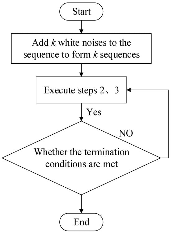
Figure 1.
Schematic representation of the CEEMDAN process.
2.2. MIC Algorithm
The MIC, introduced in 2011, offers notable benefits in assessing both linear and nonlinear relationships among variables without being constrained to particular functions. Despite minimal impact from anomalies, MIC could still precisely uncover intricate correlations within the information. The fundamental concept of MIC involves mapping two random variables onto a two-dimensional space and conducting grid partitioning. Specifically, for a given dataset D = {(Ai, Bi), i = 1, 2, …, n}, where A and B represent variables in D, these information points are projected onto a two-dimensional graph and gridded relying on the coordinate axes, generating a grid graph G(x, y). Within this grid graph, information points are distributed across different grids, and the allocation in different grids may differ. To accurately gauge the association between variables and better comprehend the potential connection between two random variables, it is essential to compute the mutual information under diverse distributions and identify the maximum value among them, as depicted in Equation (6).
where MI(D|G) signifies the mutual information value of the dataset D given grid G. To analyze information at different scales, it is crucial to standardize all maximum mutual information scores under different partitions, as illustrated in Equation (7).
The MIC is the highest value of M(D)x,y obtained under diverse partitions. The calculation formula is expressed as
The formula incorporates B(n), which denotes the upper limit of the number of partition grids. It is generally optimal to set B(n) = n0.6. The MIC ranges from 0 to 1. A substantial MIC value between feature and target variables indicates a robust correlation; thus, the feature variable should be retained. An MIC value near 0 indicates weak or no correlation; thus, the feature variable should be eliminated. Moreover, if the MIC scores between different feature variables are close to 1, then this value implies a high correlation, indicating strong redundancy and high substitutability. Conversely, if the MIC value is close to 0, then this value indicates complete independence and no redundancy. The specific criteria for MIC in determining correlation are presented in Table 1.

Table 1.
Comparison of MIC value range and variable correlation degree.
The MIC approach is employed in the domain of wind power forecasting to calculate all MIC scores of different weather features and rank their input vectors based on numerical differences. According to the ranking outcomes, a specific number of weather features are selected for the forecasting model, and the original weather feature information is dimensionally reduced to enhance wind power forecasting speed, minimize redundant information, and consequently improve forecasting accuracy.
2.3. LSTM Algorithm
The LSTM network, a specialized variant of the recurrent neural network, effectively addresses the issues in vanishing and exploding gradients that emerge during the training of lengthy sequences, including wind power data. An LSTM architecture typically comprises the following four fundamental components: an input gate, a forget gate, an output gate, and a memory cell. The memory cell performs element-wise multiplication to remove irrelevant information and reduce model complexity. The input gate integrates information from the current and previous time steps, facilitating the transmission of pertinent information to the memory cell. The output gate regulates the memory cell’s transmission of useful information to the hidden layer, serving as input for the subsequent time step. Figure 2 depicts the computational flow of the LSTM network, accounting for an input sequence xt and an output sequence yt.

Figure 2.
Architectural diagram of the LSTM network.
As shown in Figure 2, ht represents the hidden layer vector at time step t, while ct denotes the cell state at the same time step t. The matrices Wf, Wi, Wo, and Wc correspond to the weight matrices for the forget gate, input gate, output gate, and cell state at time step t, respectively, all of which are activated by the Sigmoid activation function. The mathematical equations for the input gate it, forget gate ft, and output gate ot are
where bi, bf, and bo represent the biases associated with the three gates, σ is the Sigmoid activation function.
At time step t, the formula for updating the cell state is given by
where ⊙ denotes the Hadamard product.
where bc represents the bias term.
Finally, the hidden layer vector is updated as follows:
where φ represents the activation function.
Thus, the following could be obtained:
where Wf represents the adjustable weight matrix, while by represents the bias term.
3. The NWP-CEEMDAN-LSTM Approach for Wind Power Forecasting
3.1. Normalization
Given the highly volatile nature of wind power, normalizing wind power and other related information is necessary to ensure a consistent measurement scale, thereby enhancing the applicability of the proposed approach. Information normalization involves the transformation of all information points into a range between [0, 1] using different processing techniques. The objective is to eliminate the discrepancies in magnitude between different information sets and prevent substantial forecasting errors in the network due to considerable variations in input and output information magnitudes. The information normalization process is represented by Equation (16).
where xmin denotes the minimum value in the information sequence, while xmax represents the maximum value.
After forecasted data generation, the outcomes are obtained in a normalized form. Applying inverse normalization to the forecasted output data is necessary to retrieve the information in its original format. The inverse normalization process pertains to the reverse of the corresponding normalization process applied initially.
3.2. NWP Feature Information Selection Based on MIC
Considering the complex coupling relationship between wind power output and meteorological factors, the information from meteorological characteristics can effectively improve the forecast accuracy. However, redundant features with minimal influence may cause model interference and increase model complexity, thus affecting the forecast accuracy. Therefore, quantitatively analyzing the correlation between input features and output power, screening reasonable features to retain effective information, reducing feature complexity, and offering high-quality data support for subsequent model construction are necessary. The MIC method has remarkable advantages in evaluating linear and nonlinear relationships between variables without being limited to a specific function. This method can also accurately uncover the complex correlation between data, receiving minimal effects from outliers. Therefore, the maximum MIC is used to select the appropriate input weather feature vector to improve the accuracy of the forecast results.
Using the MIC technique for feature selection, this study evaluated six meteorological variables: wind velocity, wind orientation, atmospheric temperature, barometric pressure, relative humidity, and air density. The NWP data used in this article is the adapted data from the relevant wind farms, offering data support for the power prediction of the wind farms in this article. Table 2 presents the MIC values of different meteorological variables.
Table 2.
MIC values of different meteorological variables.
Although the MIC feature analysis approach has yielded a prioritization of different weather characteristics, the optimal quantity of feature vectors to input for achieving the best outcomes remains uncertain. Consequently, in this section, some sampling points are selected for wind power prediction. According to the degree of the correlation between weather characteristics and wind power, different numbers of weather features are selected to conduct error analysis on multiple prediction results. The Mean Absolute Percentage Error (MAPE) evaluation metric serves as the criterion for determining the ideal number of input vectors. The LSTM algorithm was adopted as the short-term wind power prediction method, and the average error results of multiple predictions are shown in Figure 3.
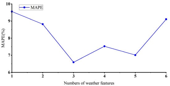
Figure 3.
The average MAPE of LSTM with different numbers of weather features.
As shown in Figure 3, when wind speed, wind direction, and air pressure occupy the top three positions among the input feature vectors, the MAPE value reaches its minimum. Thus, the most optimal approach involves the selection of the three variables as the input feature vectors. Moreover, when the input feature vector comprises five elements, the wind power forecasting error is reduced compared to the scenario where the input feature vector containing four elements. This reduction is attributed to humidity solely acting as a weather feature, revealing a weak correlation with power. However, this feature can affect the surface condition of the wind turbine blades, thereby influencing aerodynamic performance and generating a positive feedback on the prediction results. When the input feature vector contains four elements, the error exceeds that of the three-element case.
This observation highlights the importance of carefully selecting the quantity of distinct weather features in error analysis.
3.3. NWP-CEEMDAN-LSTM Model
The suggested NWP-CEEMDAN-LSTM approach for short-term wind power forecasting encompasses several key stages, which are delineated as follows:
- The historical wind power and NWP information is standardized to ensure consistency.
- The normalized historical data of wind power is used as the input of the CEEMDAN algorithm, and the wind power data with large volatility is decomposed into k sub-modal signals with small volatility through the CEEMDAN algorithm.
- The MIC values of various NWP data are calculated, and the input weather feature vectors are sorted in accordance with the numerical differences. Using the sorting results, the number of weather features in the forecast model was selected, and the original NWP data was reduced to eliminate redundant information.
- The sequences after modal decomposition and the NWP data selected by MIC features are used as inputs to the LSTM forecast algorithm.
- The k forecasting outcomes are aggregated and reconstructed to acquire the wind power forecasting data.
- Inverse standardization is applied to the forecasting scores obtained in step 5 to determine the actual wind power forecasting data. A comparative analysis between the forecasted and expected scores is performed to assess the errors.
Figure 4 illustrates the detailed workflow of the proposed NWP-CEEMDAN-LSTM approach for short-term wind power forecasting.
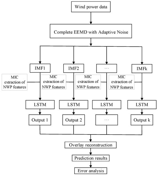
Figure 4.
Detailed flowchart for the NWP-CEEMDAN-LSTM approach.
3.4. Evaluation Criteria
After the forecasting model generates the forecast outcomes, comparing these results with the actual information and using error evaluation metrics are essential to assess the performance of different forecasting models. Aiming to ensure a standardized evaluation of model effectiveness and accuracy, this study uses three assessment metrics: root mean square error (RMSE), mean absolute error (MAE), and MAPE, as represented by Equations (17), (18), and (19), respectively.
where m signifies the number of wind power sampling points, yi denotes the forecast wind power generation, and yi′ denotes the actual wind power generation.
4. Case Study
In this study, historical information from six different wind farms is the experimental data (including wind power, temperature, air pressure, humidity, wind speed, wind direction and humidity), and the sampling interval of these data is 15 min. The specification parameters of six different wind farms are shown in Table 3. Each wind farm selects 1000 datasets to ensure the accuracy of the proposed method, including 800 training datasets and 200 verification datasets. MATLAB 2021a was used for wind power prediction.
Table 3.
Specification parameters of wind farms.
4.1. Decomposition Results of CEEMDAN
The CEEMDAN algorithm was applied to the normalized wind power data, and the resulting IMF components serve as input for the short-term wind power forecasting approach introduced in the study. Figure 5 shows the specific decomposition outcomes.
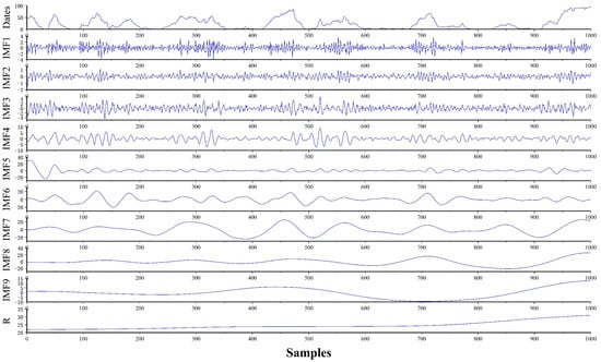
Figure 5.
Decomposition outcome chart of CEEMDAN.
As shown in Figure 5, the CEEMDAN algorithm effectively decomposes the highly volatile wind power generation information into nine IMF components, demonstrating progressively decreasing frequencies and one residual component. These less fluctuating modal signals reduce the forecast error of the model after input to the forecast model. This reduction is attributed to the evident regularity, revealing markedly reduced ranges of value changes.
4.2. Selection of Weather Characteristics for Different IMF Components
Aiming to optimize model input and enhance prediction performance, this section identifies meteorological features that provide substantial contributions to prediction results by calculating the MIC values between each IMF component and various meteorological features. Using these meteorological features as input data for the model not only reduces model complexity, but also enhances the speed and accuracy of prediction. Based on in-depth analysis and the comparison of MIC values, the correlation strength between each meteorological feature and the IMF component of wind power is illustrated in Figure 6.
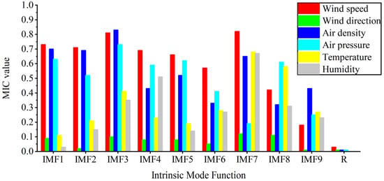
Figure 6.
Bar chart of MIC values for different weather characteristics with various IMF components.
As shown in Figure 6, considerable differences are observed in the correlation between different meteorological parameters and IMF components. Therefore, during construction of a wind power prediction model, selecting appropriate input parameters based on the actual situation is necessary to improve the accuracy and reliability of the prediction results.
Aiming to further analyze the potential impact of changes in the number of weather features adopted by different IMF components on the final prediction accuracy, and to clarify the optimal weather feature vector size input, this section will select different numbers of weather features as input variables based on MIC values from high to low. Prediction and error analysis for each IMF component will also be conducted separately. Based on the previous research in Section 4.2, a preliminary exploration on the relationship between the prediction error of raw wind power output data and the number of weather feature vectors in the input model is performed in this study. This section will further focus on each IMF component, according to the principle of the correlation between weather characteristics and wind power, analyze the impact of the number of input feature vectors on the prediction results, and determine the MAPE value of the prediction results, as shown in Figure 7.
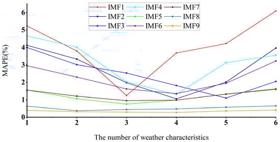
Figure 7.
Prediction error analysis of different IMFs with different numbers of weather characteristics.
As shown in Figure 7, the MAPE values of the predicted results for different IMF components substantially vary under different numbers of characteristic weather conditions. Therefore, selecting the number of effective weather features has a remarkable impact on the predicted results. In this figure, the minimum MAPE value of the predicted modal component IMF1 of wind power corresponds to the number of three weather features. The minimum MAPE value of the predicted modal component IMF2 of wind power corresponds to the number of four weather features. The minimum MAPE value of the predicted modal component IMF3 of wind power corresponds to the number of five weather features. The minimum MAPE value of the predicted modal component IMF4 of wind power corresponds to the number of four weather features. The minimum MAPE value of the predicted modal component IMF5 of wind power corresponds to the number of three weather features. The minimum MAPE value of the predicted modal component IMF6 of wind power corresponds to the number of four weather features. The minimum MAPE value of the predicted modal component IMF7 of wind power corresponds to the number of three weather features. The minimum MAPE value of the predicted modal component IMF8 of wind power corresponds to the number of two weather features. The minimum MAPE value of the predicted modal component IMF9 of wind power corresponds to the number of four weather features.
The weather feature vectors with high correlation, eliminated via MIC feature selection, were used as input vectors to predict the IMF components of wind power. After the prediction, the prediction results of nine different IMF components were obtained. IMF2 and IMF5 were selected as display samples, and the result graphs obtained after prediction are shown in Figure 8 and Figure 9.
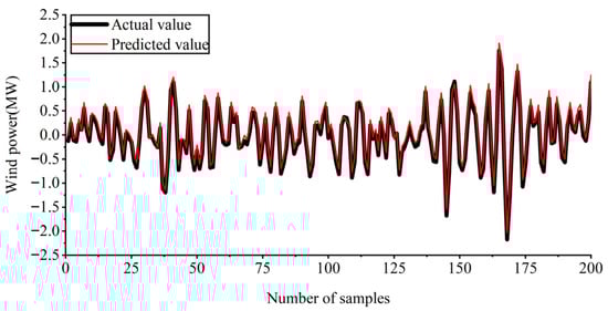
Figure 8.
Prediction results of IMF2.
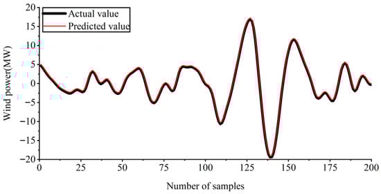
Figure 9.
Prediction results of IMF5.
Figure 8 and Figure 9 show the predicted results of IMF2 and IMF5, respectively, while the predicted results of other wind power components are similar. The prediction results in the figure reveal relatively small errors between the predicted and true values of each wind power component. Therefore, the accuracy of the wind power prediction model is effectively improved by selecting different numbers of weather features as input vectors for each wind power component using MIC.
4.3. Validation of NWP-CEEMDAN-LSTM
Aiming to verify the effectiveness and accuracy of the proposed method in this paper, four methods (BP, LSTM, NWP-LSTM, and NWP-EEMD-LSTM) were used for forecasting, and the forecast results were compared and analyzed.
4.3.1. Forecast Results of BP
Figure 10 reveals that, although the BP algorithm could track the turning points of actual wind power generation, it still struggles to adapt to the fluctuations in wind power generation. Within some instances, the forecasting outcomes of the BP algorithm even demonstrate opposite conclusions at actual power fluctuation turning points, indicating considerable deviations in the forecasted outcomes. Consequently, the BP algorithm fails to provide reliably accurate support for short-term wind power generation forecasting.
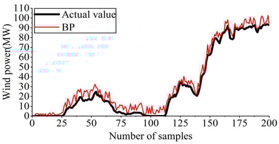
Figure 10.
Forecasting outcomes of BP.
4.3.2. Forecast Results of LSTM
The experimental outcomes in Figure 11 indicate that the LSTM approach improves forecasting accuracy compared to the BP algorithm. LSTM also exhibits effectively tracking of actual power generation fluctuations. However, this approach lacks adaptability to information with frequent fluctuations. Aiming to address this issue, the next step in this study involves employing NWP-LSTM for training and forecasting on the relevant data.
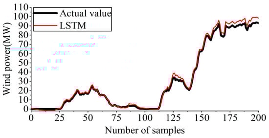
Figure 11.
Forecasting outcomes of LSTM.
4.3.3. Forecast Results of NWP-LSTM
As depicted in Figure 12, the experimental outcomes indicate that the NWP-LSTM approach demonstrates good tracking performance for information with frequent fluctuations. However, a notable error in forecasting outcomes is observed at nodes with frequent fluctuations in wind power generation.
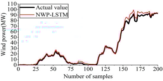
Figure 12.
Forecasting outcomes of NWP-LSTM.
4.3.4. Forecast Results of NWP-CEEMD-LSTM
The experimental outcomes presented in Figure 13 reveal that the NWP-EEMD-LSTM approach not only effectively tracks fluctuations in wind power generation, but also achieves high forecasting accuracy. The maximum forecasting error in the experiment is 1.56 MW. This result indicates that the mode mixing problem, associated with the EEMD approach, could affect the decomposition results and consequently impact the accuracy of all forecasting outcomes.

Figure 13.
Forecasting outcomes of NWP-CEEMD-LSTM.
4.3.5. Forecast Results of NWP-CEEMDAN-LSTM
The experimental outcomes illustrated in Figure 14 demonstrate that the NWP-CEEMDAN-LSTM approach effectively tracks actual power fluctuations while ensuring good forecasting information accuracy.
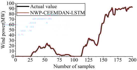
Figure 14.
Forecasting outcomes of NWP-CEEMDAN-LSTM.
As presented in Table 4, the MAE, RMSE, and MAPE scores of the proposed NWP-CEEMDAN-LSTM method, which considers MIC feature extraction, are substantially lower compared to the BP, LSTM, NWP-LSTM, and NWP–CEEMD–LSTM forecasting approaches. This finding indicates that, compared to other approaches, the proposed wind power forecasting approach in the study has stronger accuracy and adaptability. Furthermore, CEEMD is effective in reducing the impact of signal fluctuations and intermittency on the signal.
Table 4.
Evaluation results of different forecasting methods.
4.4. Superiority Verification of NWP-CEEMDAN-LSTM
Aiming to verify the superiority of the proposed method, the forecast results were compared with those of three different combination methods (NWP-CNN-GRU, VMD-PSO-LSSVM, and IWOA-SA-Elman).
The experimental results in Figure 15 indicate relatively accurate forecast results of the NWP-CNN-GRU, VMD-PSO-LSSVM, and IWOA-SA-Elman methods. However, its forecast accuracy is inferior to that of the NWP-CEEMDAN-LSTM methods. The experimental results reveal the advantages of the NWP-CEEMDAN-LSTM method in the short-term forecast of wind power. The evaluation results presented in Table 5 support this conclusion.
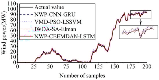
Figure 15.
Forecasting outcomes of different combination forecasting methods.
Table 5.
Evaluation results of different combination forecasting methods.
4.5. Universality Verification of NWP-CEEMDAN-LSTM
Aiming to verify the universality of the proposed method, the wind power of other wind farms in different geographical locations will be predicted and analyzed. Figure 16 shows the number of weather features selected using MIC corresponding to the IMF components of wind power at two different geographical locations. Figure 17 shows the short-term prediction results of wind power for wind farms in two different geographical locations.
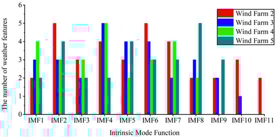
Figure 16.
The number of weather features of IMF components of different wind power.
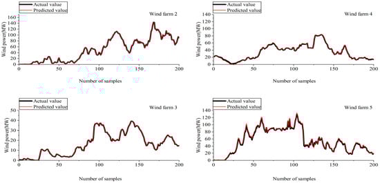
Figure 17.
Forecasting outcomes of different wind farms.
The number of weather features in Figure 16 reveals the minimum number of MAPE values for each IMF component of wind power. In this table, during wind power prediction for wind farms at different locations, the number of selected weather features using MIC for the IMF component of each wind power shows different situations due to the influence of the geographical and climatic environments of each wind power site.
As shown in Figure 17, the wind power prediction results of the four wind farms at different locations both demonstrate a good state. At the points with rapid wind power fluctuations, it can still follow these fluctuations and ensure accurate predictions. Among them, the maximum errors in wind power prediction for the four wind farms are 0.61 MW, 0.42 MW, 0.54 MW and 1.03 MW. The prediction results in Figure 17 indicate that the NWP-CEEMDAN-LSTM proposed in this paper, which accounts for MIC feature selection, demonstrates universality for short-term wind power prediction of wind farms at various locations.
As shown in Figure 18, the prediction errors of wind power vary in different seasons. The error is the smallest in summer, which is because the wind speed is relatively stable in summer. In winter, cold air activities are frequent, wind speeds are high and variable, which increases the uncertainty of predictions and thus leads to the greatest error in winter. The maximum errors of wind power prediction in different seasons are 1.12 MW, 0.62 MW, 1.51 MW and 1.93 MW. It can be seen from the prediction results in Figure 18 that the NWP-CEEMDAN-LSTM considering MIC feature selection proposed in this paper also has good accuracy in the short-term wind power prediction of wind farms in different seasons.
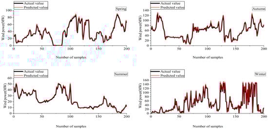
Figure 18.
Forecasting outcomes of wind power in different seasons.
5. Conclusions
This study proposes a wind power forecasting approach based on the NWP-CEEMDAN-LSTM algorithm, using MIC feature extraction for short-term wind power forecasts. A comparison of the experimental results with different methods and farms yields the following conclusions:
- This paper investigates the challenge of wind power prediction accuracy caused by the intermittent and non-stationary nature of wind power generation. To address this issue, the Complete Ensemble Empirical Mode Decomposition with Adaptive Noise (CEEMDAN) algorithm is employed to decompose historical wind power data into multiple intrinsic mode functions (IMFs). These subsequences serve as inputs to a Long Short-Term Memory (LSTM) network for individual prediction. Simulation results demonstrate that CEEMDAN effectively mitigates the influence of residual white noise in the data sequences on the forecasting process, thereby enhancing the accuracy of wind power prediction.
- Furthermore, to counteract the potential adverse effects of high-dimensional weather features on prediction performance, this study applies the Maximal Information Coefficient (MIC) to evaluate the correlation between Numerical Weather Prediction (NWP) data and wind turbine output power. Feature types and dimensions are selectively determined for each wind power subsequence based on their correlation ranking. Experimental results indicate that the MIC-based feature selection reduces the impact of NWP data redundancy and improves prediction reliability.
- Through comparative experiments with various models—including BP, LSTM, CEEMDAN-LSTM, NWP-LSTM, and the proposed NWP-CEEMDAN-LSTM—this study validates that the proposed method effectively tracks wind power fluctuations and reduces prediction errors. Additional benchmarking against NWP-CNN-GRU, VMD-PSO-LSSVM, and IWOA-SA-Elman models confirms the superior prediction accuracy of the proposed framework. Moreover, tests under different geographical and seasonal conditions verify the generalizability and robustness of the method.
Next, the optimal weather feature set for different IMFs will be determined using methods such as model performance evaluation based on cross-validation and iterative feature selection. Future research should consider the application of the NWP-CEEMDAN-LSMT algorithm in the wind farm cluster.
Author Contributions
Writing—original draft preparation, Y.Y.; supervision, Y.Z. All authors have read and agreed to the published version of the manuscript.
Funding
This research received no external funding.
Data Availability Statement
The data presented in this study are available on request from the corresponding authors. The data are not publicly available due to confidentiality agreements.
Conflicts of Interest
The authors declare no conflicts of interest.
References
- Global Wind Energy Council. Global Wind Report 2025. In Proceedings of the Offshore Wind Power Conference 2025, Da Lian, China, 20 June 2025; Available online: https://www.gwec.net/reports/globalwindreport (accessed on 30 August 2025).
- Wu, Q.; Zheng, H.; Guo, X.; Liu, G. Promoting wind energy for sustainable development by precise wind speed prediction based on graph neural networks. Renew. Energy 2022, 199, 977–992. [Google Scholar] [CrossRef]
- Zhang, Y.; Shi, J.; Li, J.; Yun, S. Short-Term Wind Speed Prediction Based On Residual and VMD-ELM-LSTM. Acta Energ. Sol. Sin. 2023, 44, 340–347. [Google Scholar]
- Zhang, Y.; Zhao, Y.; Shen, X.; Zhang, J. A comprehensive wind speed prediction system based on Monte Carlo and artificial intelligence algorithms. Appl. Energy 2022, 305, 117815. [Google Scholar] [CrossRef]
- Peng, X.; Cheng, K.; Lang, J.; Zhang, Z.; Cai, T.; Duan, S. Short-Term Wind Power Prediction for Wind Farm Clusters Based on SFFS Feature Selection and BLSTM Deep Learning. Energies 2021, 14, 1894. [Google Scholar] [CrossRef]
- Wang, L.; Wei, L.; Liu, J.; Qian, F. A probability distribution model based on the maximum entropy principle for wind power fluctuation estimation. Energy Rep. 2022, 8, 5093–5099. [Google Scholar] [CrossRef]
- Sun, M.; Feng, C.; Zhang, J. Conditional aggregated probabilistic wind power forecasting based on spatio-temporal correlation. Appl. Energy 2019, 256, 113842. [Google Scholar] [CrossRef]
- Sun, Y.; Wang, P.; Zhai, S.; Hou, D.; Wang, S.; Zhou, Y. Ultra short-term probability prediction of wind power based on LSTM network and condition normal distribution. Wind. Energy 2020, 23, 63–76. [Google Scholar] [CrossRef]
- Xu, T.; Du, Y.; Li, Y.; Zhu, M.; He, Z. Interval prediction method for wind power based on VMD-ELM/ARIMA-ADKDE. IEEE Access 2022, 10, 72590–72602. [Google Scholar] [CrossRef]
- Godinho, M.; Castro, R. Comparative performance of AI methods for wind power forecast in Portugal. Wind. Energy 2021, 24, 39–53. [Google Scholar] [CrossRef]
- Tian, W.; Bao, Y.; Liu, W. Wind power forecasting by the BP neural network with the support of machine learning. Math. Probl. Eng. 2022, 2022, 7952860. [Google Scholar] [CrossRef]
- Peng, Y.; Xiang, W. Short-term traffic volume prediction using GA-BP based on wavelet denoising and phase space reconstruction. Phys. A Stat. Mech. Its Appl. 2020, 549, 123913. [Google Scholar] [CrossRef]
- Lu, P.; Li, Y.; Zhong, W.; Qu, Y.; Tang, Y.; Zhao, Y. A novel spatio-temporal wind power forecasting framework based on multi-output support vector machine and optimization strategy. J. Clean. Prod. 2020, 254, 119993. [Google Scholar] [CrossRef]
- Ding, M.; Zhou, H.; Xie, H.; Wu, M.; Liu, K.; Nakanishi, Y. A time series model based on hybrid-kernel least-squares support vector machine for short-term wind power forecasting. ISA Trans. 2021, 108, 58–68. [Google Scholar] [CrossRef]
- Wang, Y.; Wang, D.; Tang, Y. Clustered hybrid wind power prediction model based on ARMA, PSO-SVM, and clustering methods. IEEE Access 2020, 8, 17071–17079. [Google Scholar] [CrossRef]
- Gao, X.; Guo, W.; Mei, C.; Sha, J.; Guo, Y.; Sun, H. Short-term wind power forecasting based on SSA-VMD-LSTM. Energy Rep. 2023, 9, 335–344. [Google Scholar] [CrossRef]
- Sun, Z.; Zhao, M. Short-term wind power forecasting based on VMD decomposition, ConvLSTM networks and error analysis. IEEE Access 2020, 8, 134422–134434. [Google Scholar] [CrossRef]
- Zhao, Z.; Yun, S.; Jia, L.; Guo, J.; Yao, M.; He, N.; Li, X. Hybrid VMD-CNN-GRU-based model for short-term forecasting of wind power considering spatio-temporal features. Eng. Appl. Artif. Intell. 2023, 121, 105982. [Google Scholar] [CrossRef]
- Sun, Z.; Zhao, S.; Zhang, J. Short-term wind power forecasting on multiple scales using VMD decomposition, K-means clustering and LSTM principal computing. IEEE Access 2019, 7, 166917–166929. [Google Scholar] [CrossRef]
- Ding, Y.; Chen, Z.; Zhang, H.; Wang, X.; Guo, Y. A short-term wind power prediction model based on CEEMD and WOA-KELM. Renew. Energy 2022, 189, 188–198. [Google Scholar] [CrossRef]
- Yu, C.; Yan, G.; Yu, C.; Zhang, Y.; Mi, X. A multi-factor driven spatiotemporal wind power prediction model based on ensemble deep graph attention reinforcement learning networks. Energy 2023, 263, 126034. [Google Scholar]
- Shi, P.; Wei, X.; Zhang, C.; Xie, L.; Ye, J.; Yang, J. Short-term wind power prediction based on VMD-BOA-LSSVM-AdaBoost. Acta Energ. Sol. Sin. 2024, 45, 226–233. [Google Scholar]
- Liu, J.; Zhu, X.; Yu, J. Short-term wind power prediction based on IWOA-SA-ELMAN neural network. Acta Energ. Sol. Sin. 2024, 45, 143–150. [Google Scholar]
- Xiong, Z.; Chen, Y.; Ban, G.; Zhuo, Y.; Huang, K. A Hybrid Algorithm for Short-Term Wind Power Prediction. Energies 2022, 15, 7314. [Google Scholar] [CrossRef]
- Yan, Y.; Wang, X.; Ren, F.; Shao, Z.; Tian, C. Wind speed prediction using a hybrid model of EEMD and LSTM considering seasonal features. Energy Rep. 2022, 8, 8965–8980. [Google Scholar] [CrossRef]
- Lian, L. Wind speed prediction based on CEEMD-SE and multiple echo state network with Gauss–Markov fusion. Rev. Sci. Instrum. 2022, 93, 015105. [Google Scholar] [CrossRef]
Disclaimer/Publisher’s Note: The statements, opinions and data contained in all publications are solely those of the individual author(s) and contributor(s) and not of MDPI and/or the editor(s). MDPI and/or the editor(s) disclaim responsibility for any injury to people or property resulting from any ideas, methods, instructions or products referred to in the content. |
© 2025 by the authors. Licensee MDPI, Basel, Switzerland. This article is an open access article distributed under the terms and conditions of the Creative Commons Attribution (CC BY) license (https://creativecommons.org/licenses/by/4.0/).