A Novel Fault Detection Scheme Based on Mutual k-Nearest Neighbor Method: Application on the Industrial Processes with Outliers

Abstract

The k-nearest neighbor (kNN) method only uses samples’ paired distance to perform fault detection. It can overcome the nonlinearity, multimodality, and non-Gaussianity of process data. However, the nearest neighbors found by kNN on a data set containing a lot of outliers or noises may not be actual or trustworthy neighbors but a kind of pseudo neighbor, which will degrade process monitoring performance. This paper presents a new fault detection scheme using the mutual k-nearest neighbor (MkNN) method to solve this problem. The primary characteristic of our approach is that the calculation of the distance statistics for process monitoring uses MkNN rule instead of kNN. The advantage of the proposed approach is that the influence of outliers in the training data is eliminated, and the fault samples without MkNNs can be directly detected, which improves the performance of fault detection. In addition, the mutual protection phenomenon of outliers is explored. The numerical examples and Tenessee Eastman process illustrate the effectiveness of the proposed method.

1. Introduction

Data are being generated all the time in industrial processes. Since industry became a separate category from social production, data collection and use in industrial production has gradually increased. In this context, data-driven multivariate statistical process monitoring (MSPM) methods have developed leaps and bounds [1,2], where principal component analysis (PCA) methods are the most widely used [3,4,5,6]. However, there are cases where PCA-based fault detection methods do not perform well. For example, the detection threshold of Hotelling-$T^2$ and squared prediction error (SPE) are calculated based on the premise that process variables satisfy a normal or Gaussian distribution. Due to the nonlinearity, non-Gaussianity, and multimodality in industrial processes, it is not easy to meet this assumption in practice [7,8,9,10,11]. Therefore, the traditional PCA-based process monitoring method has poor monitoring performance when facing the above problems [12,13,14,15,16].

He and Wang [11] proposed a non-parametric lazy fault detection method based on the k-nearest neighbor rule (FD-kNN) to deal with the above problems. The main idea is to measure the difference between samples by distance; that is the online normal samples and training samples are similar, but fault samples and training samples are significantly different. It only uses samples’ paired distance to perform fault detection and has no strict requirements for data distribution. Hence, this method provide an alternative way to overcome the nonlinearity, non-Gaussianity, multimodality in industrial processes.

However, the data collected in the actual industrial process usually contain a certain amount of noise and even outliers, and the quality of the data cannot be guaranteed [17,18]. Outliers are generally those samples that are far from the normal training samples and tend to behave statistically inconsistent with the other normal samples [19,20]. In the actual industrial processes, outliers are usually introduced when measurement or recording errors are made. In addition, the considerable process noise is also one of the main reasons for the generation of outliers [20].

The neighbors of the samples found by kNN from a data set containing noises or outliers may not be actual neighbors but a pseudo-nearest neighbor (PNN). For example, in Figure 1, the samples $x_2$, $x_3$, and $x_4$ are the 3-NNs of $x_1$, but sample $x_1$ is not one of the 3-NNs of $x_2$, $x_3$, and $x_4$. In other words, $x_2$, $x_3$, and $x_4$ are the PNNs of $x_1$. This interesting phenomenon can be explained with an example from human interaction: I regard you as one of my best friends, but I am not among your best friends. As can be seen from Figure 1, the sample $x_1$ is far away from its pseudo-neighbors so that the detection threshold calculated by the pseudo-neighbors in the training phase will have a significant deviation, which will seriously degrade the detection performance of the FD-kNN.

While there are many techniques for removing outliers, these data preprocessing methods make the model building extraordinarily time-consuming and labor-intensive [21,22].

In this paper, a novel fault detection method using the mutual kNN rule (FD-MkNN) is proposed. Finding nearest neighbors using the mutual k-nearest neighbor rule will exclude the influence of PNNs (see Section 2.2.1 for the definition of mutual k-nearest neighbor (MkNN)). Before the model is established, the outliers in the training set are eliminated by the MkNN method, and the data quality for monitoring is improved. In the stage of fault detection, if the test sample does not have mutual neighbors, it is judged to be faulty. For test samples with mutual neighbors, the corresponding distance statistics are calculated to perform process monitoring. Compared with the FD-kNN, MkNN uses more valuable and truthful information (i.e., neighbors of the sample’s neighbors), which improves the performance of process monitoring. The main contributions of this paper are as follows:

• To our best knowledge, the MkNN method is proposed to perform fault detection of industrial processes with outliers for the first time;
• The proposed method simultaneously realizes the elimination of outliers and the fault detection;
• The mutual protection problem of outliers is solved.

This paper will proceed as follows. In Section 2, the FD-kNN method is first briefly reviewed and then the proposed FD-MkNN approach is presented in detail. In Section 3, the experiments on numerical examples and Tenessee Eastman process (TEP) illustrate the superiority of the proposed monitoring method. Section 4 and Section 5 are Discussion and Conclusions, respectively.

2. Methods

2.1. Process Monitoring Based on kNN Rule

The kNN method is widely used in pattern classification due to its simplicity. In December 2006, the top ten classic algorithms in data mining included kNN. FD-kNN was first proposed by He and Wang [11]. The main principle is to measure the difference between samples by distance; that is, normal samples and training samples are similar, but fault samples and training samples are significantly different.

• Training phase (determine the detection control limit):

  (1)

  Use Euclidean distance to get the kNNs of each training sample.

  $$d_{p,q}=∥{\mathrm{x}}_p-{\mathrm{x}}_q∥,p=1,\dots ,n,q\ne p$$

  (1)

  (2)

  Calculate the distance statistic $D_p^2$.

  $$D_p^2=\frac{1}{k}\sum _{q=1}^k{d}_{p,q}^2$$

  (2)

  where $D_p^2$ represents the average squared distance between the pth sample and its k neighbors, $d_{p,q}^2$ denotes the squared Euclidean distance between the pth sample and its qth nearest neighbor.

  (3)

  Establish the control limit $D_{\alpha }^2$ for fault detection. There are many ways to estimate $D_{\alpha }^2$, such estimation using a noncentral chi-square distribution [11], kernel density estimation (KDE). The method proposed in this paper uses the ($1-\alpha$)-empirical [23] quartile of $D_p^2$ as the threshold.

  $$D_{\alpha }^2=D_{\left(⌊n\left(1-\alpha \right)⌋\right)}^2$$

  (3)

• Detection phase:

  (1)

  For a sample $\mathrm{x}$ to be tested, find its kNNs from the training set.

  (2)

  Calculate $D_{\mathrm{x}}^2$ between $\mathrm{x}$ and its k neighbors using Equation (2).

  (3)

  Compare $D_{\mathrm{x}}^2$ with the threshold $D_{\alpha }^2$. If $D_{\mathrm{x}}^2>D_{\alpha }^2$, $\mathrm{x}$ is considered abnormal. Otherwise, it is normal.

2.2. Fault Detection Based on Mutual kNN Method

Since the nearest neighbors found by the kNN rule in the training set containing outliers may be pseudo-nearest neighbors, the fault detection threshold seriously deviates from the average level, resulting in the degradation or even failure of the monitoring performance of FD-kNN. To overcome the above problems, the concept of the mutual k-nearest neighbor (MkNN) is introduced. This section first defines MkNN and then provides the detailed steps of the proposed fault detection method.

2.2.1. MkNN

The MkNN of sample x can be defined by Equation (4). Given a sample x, if x has $x_i$ in its kNNs, $x_i$ should also have x in its kNNs [18]. According to the above definition, in Figure 1, $M_3(x_1)=\Phi$, $M_3(y_1)=\{y_2\}$, $M_3(z_1)=\{z_2,z_3\}$ and $M_3(p_1)=\{p_2,p_3,p_4\}$.

$$\begin{array}{c}\hfill M_k\left(x\right)=\left\{x_i\in D|x_i\in N_k\left(x\right)\wedge x\in N_k(x_i)\right\}\end{array}$$

(4)

where $N_k(x)$ denotes the kNNs of x, $N_k(x_i)$ represent the kNNs of $x_i$. If $M_k(x)=\Phi$, that is, x does not exist mutual kNNs. In other words, the kNNs of x are all pseudo-neighbors, and x is an outlier.

2.2.2. Proposed Fault Detection Scheme Based on Mutual kNN Method (FD-MkNN)

Before the model was established, outliers in the training set were eliminated by the MkNN method. This improves the data quality for modeling. In the fault detection stage, the relationship between samples was determined by looking for mutual nearest neighbors. If a test sample did not have mutual neighbors, this test sample was judged to be faulty. For test samples with mutual neighbors, the corresponding distance statistics were calculated to perform process monitoring. Compared with the kNN method, the proposed method uses more valuable and truthful information, improving fault detection performance. The flow chart of the proposed fault detection method is shown in Figure 2.

• Model building:

  (1)

  Finding MkNNs for each sample in the training data set $\mathrm{X}$. Eliminate the training samples that do not have any MkNNs in $\mathrm{X}$ using Equation (4). For example, if $M_k(\mathrm{x})=\Phi$, remove sample $\mathrm{x}$ from $\mathrm{X}$ and return $\mathrm{Y}$ as the final training data.

  (2)

  Calculate the MkNN average squared distance statistics of each sample in $\mathrm{Y}$ using Equation (2).

  (3)

  Determine the threshold $D_{\alpha }^2$ for fault detection using Equation (3).

• Fault detection:

  (1)

  For a sample $\mathrm{z}$ to be tested, determine whether $\mathrm{z}$ has MkNNs in $\mathrm{Y}$ using Equation (4).

  (2)

  If $\mathrm{z}$ has no MkNNs, $\mathrm{z}$ is judged as a fault sample; otherwise, go to the next step.

  (3)

  Calculate $D_{\mathrm{z}}^2$ between $\mathrm{z}$ and its MkNNs using Equation (2).

  (4)

  Compare $D_{\mathrm{z}}^2$ with the threshold $D_{\alpha }^2$. If $D_{\mathrm{z}}^2>D_{\alpha }^2$, $\mathrm{z}$ is considered faulty. Otherwise, $\mathrm{z}$ is detected as a normal sample.

2.3. Remarks

• If x is in the $q_1$th nearest neighbor of y, y is in the $q_2$th nearest neighbor of x and k = max($q_1$, $q_2$), x is the kth MNN of y and y is the kth MNN of x [24].
• The number of kNNs of sample x is k, and the number of MkNNs of x is an integer between [0, k]. Therefore, the average cumulative distance is used to calculate the distance statistics. The values of k in the outlier elimination process and fault detection stages are different, denoted as $k_1$ and $k_2$, respectively. The $k_1$ and $k_2$ are chosen according to the best cross-validation [11]. Since the value of k is more significant, the probability that the sample has MkNNs is higher. Therefore, MkNN can more easily identify outliers when the value of $k_1$ is generally smaller than $k_2$.

3. Results

In this section, numerical examples and TEP are used to explore the effectiveness of the proposed method in fault detection. In addition, the mutual protection phenomenon of outliers is explored and solved using the elbow method to improve the detection performance of FD-MkNN.

3.1. Numerical Simulation

The number of generated training samples is 300. The outliers follow the Gaussian with mean 2 and variance 2 [25], the proportion of outliers compared to the training samples is set to 0%, 1%, 2%, 3%, $4\%$, and $5\%$, respectively. In addition, there are 100 testing samples, of which the first 50 samples are normal, and the rest are faulty.

$$\begin{array}{c}x=t_1+e_1,\\ y=t_2+e_2\end{array}$$

(5)

where $t_i,i=1,2$ is a latent variable with zero mean and unit variance, and $e_i,i=1,2$ is a zero-mean noise with variance ${10}^{-4}$.

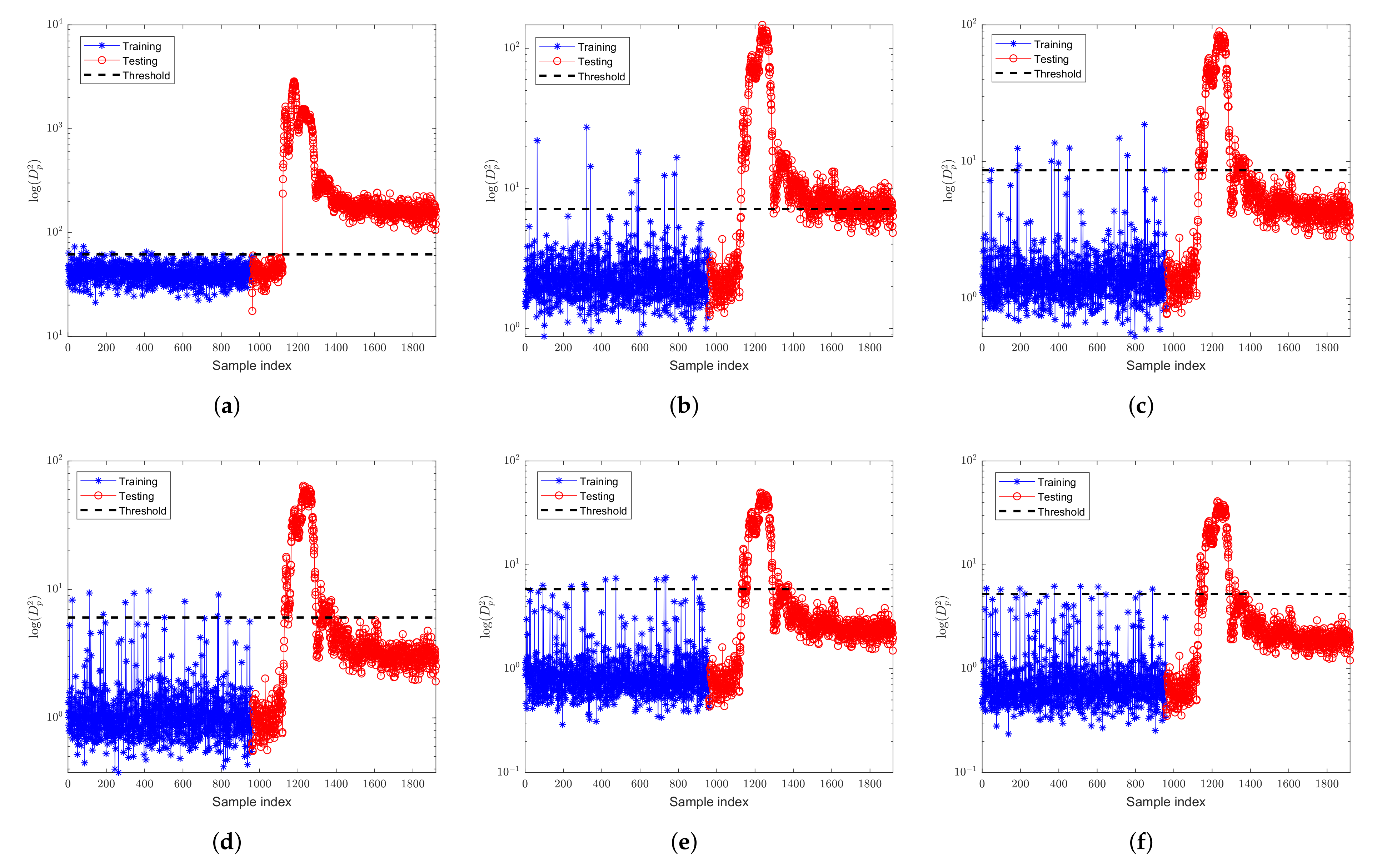
FD-kNN is first applied to detect the faults in the data set. The number of nearest neighbors is 3. At the confidence level of 99%, the detection result is shown in Figure 3. It can be seen that, as the proportion of outliers increases, the detection performance of the FD-kNN method degrades seriously. As shown in

Table 1. Fault detection rates (FDR) (%) of FD-kNN and FD-MkNN for the numerical example.

Method	No Outlier	1% Outliers	2% Outliers	3% Outliers	4% Outliers	5% Outliers
FD-kNN	100.00	98.00	74.00	62.00	46.00	20.00
FD-MkNN	100.00	100.00	94.00	84.00	80.00	76.00

, when the ratio of outliers is 5%, the fault detection rates (FDR) of the FD-kNN approach is only 20.00%. Due to outliers in the training samples, part of the neighbors of the samples found using kNN rule in the training phase are pseudo-neighbors. These pseudo-neighbors seriously affect the determination of the control threshold (that is, the control limit will be much greater than the average level) and result in poor fault detection performance.

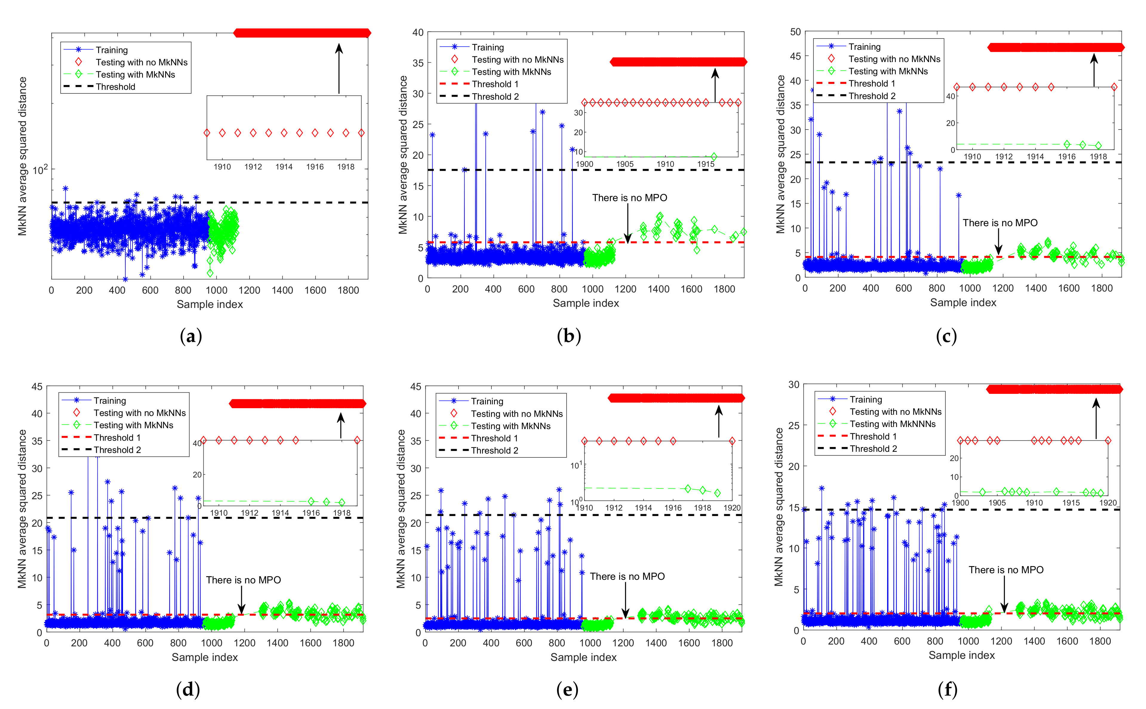
For FD-MkNN, the parameters $k_1$ and $k_2$ are set to 3 and 5, respectively. At the same confidence level (that is, $99\%$), the detection result is shown in Figure 4. As shown in Table 1, when the proportion of outliers increases from 0 to 2%, the detection performance of the FD-MkNN method is not significantly affected, and the FDR always remains above 90%. When the proportion of outliers increases from 2% to 5%, the FDR of the FD-MkNN method is significantly reduced but the FDR is always better than that of FD-kNN.

The false alarm rates (FAR) of the two methods are shown in

Table 2. False alarm rates (FAR) (%) of FD-kNN and FD-MkNN for the numerical example.

Method	No Outlier	1% Outliers	2% Outliers	3% Outliers	4% Outliers	5% Outliers
FD-kNN	0.00	0.00	0.00	0.00	0.00	0.00
FD-MkNN	0.00	2.00	4.00	4.00	0.00	2.00

(Note that the FAR is obtained based on the normal training samples). Due to outliers, the control limit or threshold of the FD-kNN method seriously deviates from the average level. Therefore, the FAR of the FD-kNN method is all zero.

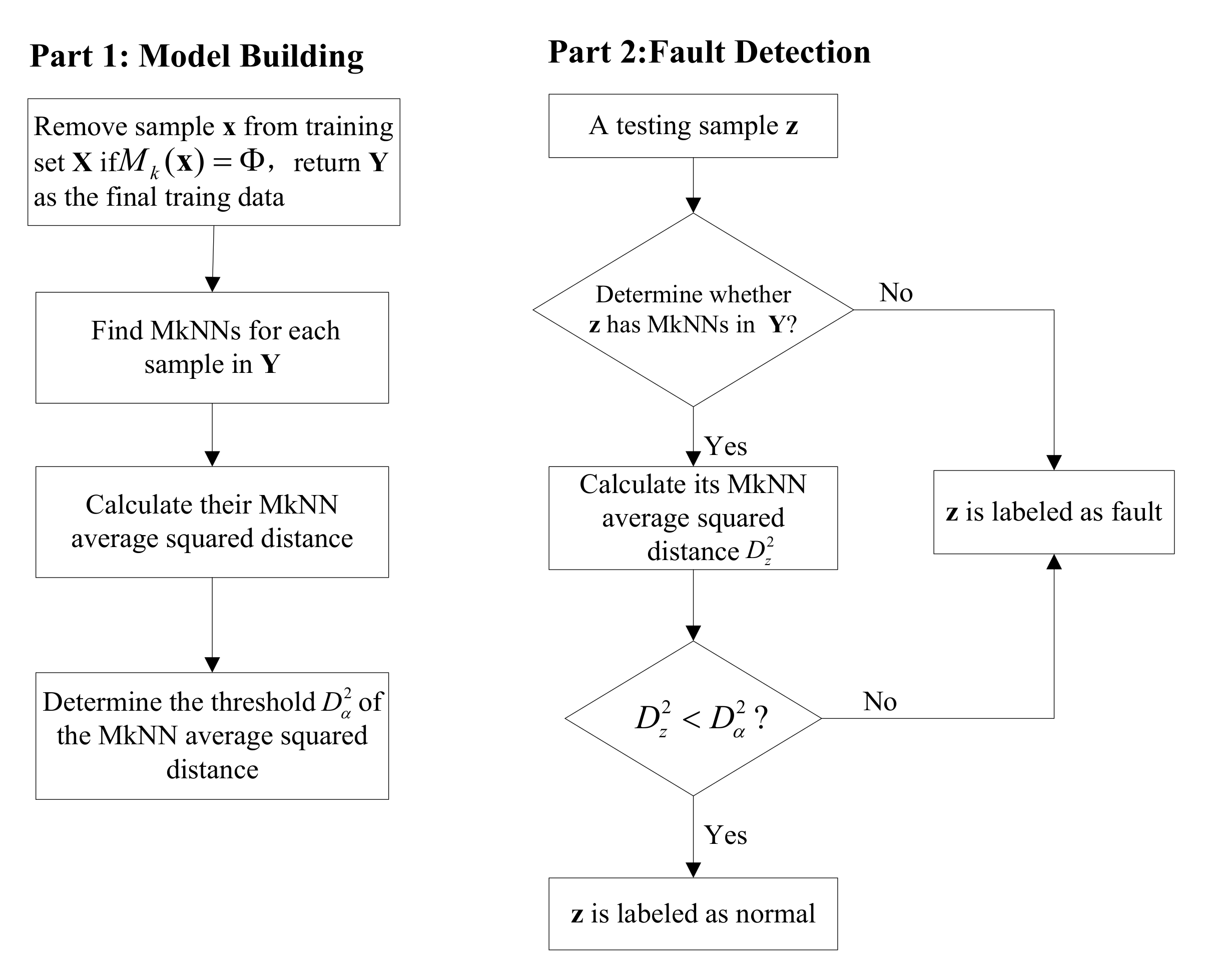
The reason why the fault detection superiority of the FD-MkNN is better than that of the FD-kNN is as follows:

• Before the training phase, part of the outliers in the training samples are removed so that the outliers will not affect the determination of the control limit in the training phase;
• In the fault detection phase, MkNN carries more valuable and reliable information than kNN. Furthermore, the effect of PNN is eliminated.

3.1.1. Experimental Results of FD-MkNN with Different Values of k

The values of k in the outlier elimination and fault detection stages are different and can be denoted as $k_1$ and $k_2$, respectively. The larger the value of k, the higher the probability that the query sample finds its mutual neighbors. Therefore, MkNN can more easily identify outliers when the value of $k_1$ is generally smaller than $k_2$. However, the value of $k_1$ cannot be too small because the MkNN method will misidentify the normal training samples as outliers and eliminate them. For example, as shown in

Table 3. Fault detection results of MkNN with different values of k for the numerical example.

${\mathit{k}}_1$	${\mathit{k}}_2$	The Number of Outliers Removed	FDR	FAR
1	3	300	-	-
3	5	33	98.00	4.00
5	7	5	86.00	0.00
7	9	2	64.00	0.00
9	11	1	52.00	0.00

, when the value of $k_1$ is set to 1, the MkNN method will eliminate all 300 training samples (the actual proportion of outliers introduced is 5%), resulting in the failure of the MkNN fault detection stages. As the value of $k_1$ increases, the number of outliers removed decreases, which makes the monitoring threshold deviate from the normal level, and the FDR decreases seriously.

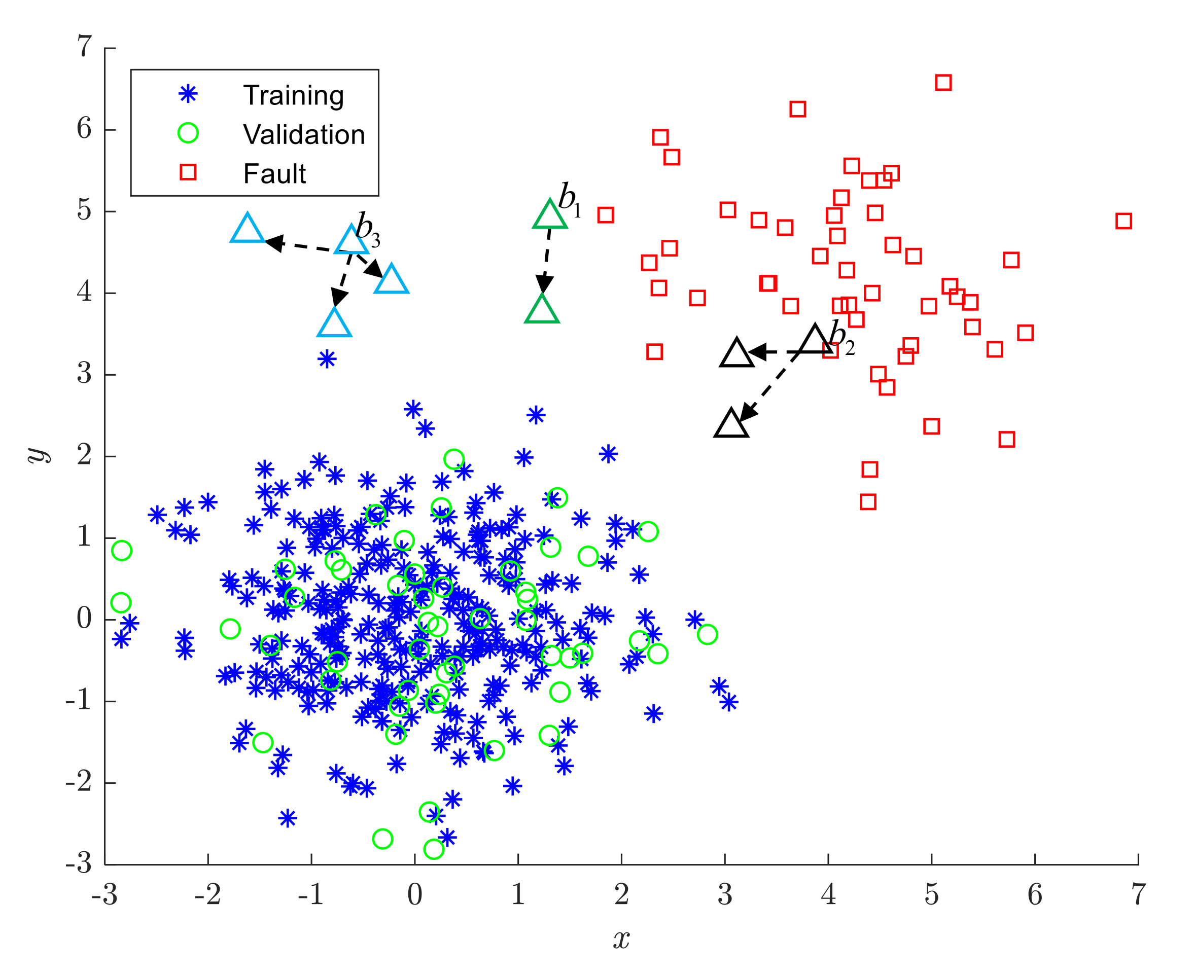
3.1.2. Mutual Protection Phenomenon of Outliers

As shown in Figure 5, when two outliers are relatively close, an interesting phenomenon will appear: they will become each other’s mutual nearest neighbors. Therefore, the MkNN rule cannot identify them as outliers. For example, in Figure 5, $b_1$, $b_2$, and $b_3$ are protected by 1, 2, and 3 outliers, respectively. When the outliers far from the normal training samples are kept in the training set due to mutual protection, it will cause the threshold or control limit calculated in the training phase to deviate seriously from the average level. We call this phenomenon the “Mutual Protection of Outliers (MPO)”, which is also the main reason why the detection performance of the FD-MkNN method decreases when the proportion of outliers increases from 2% to 5%.

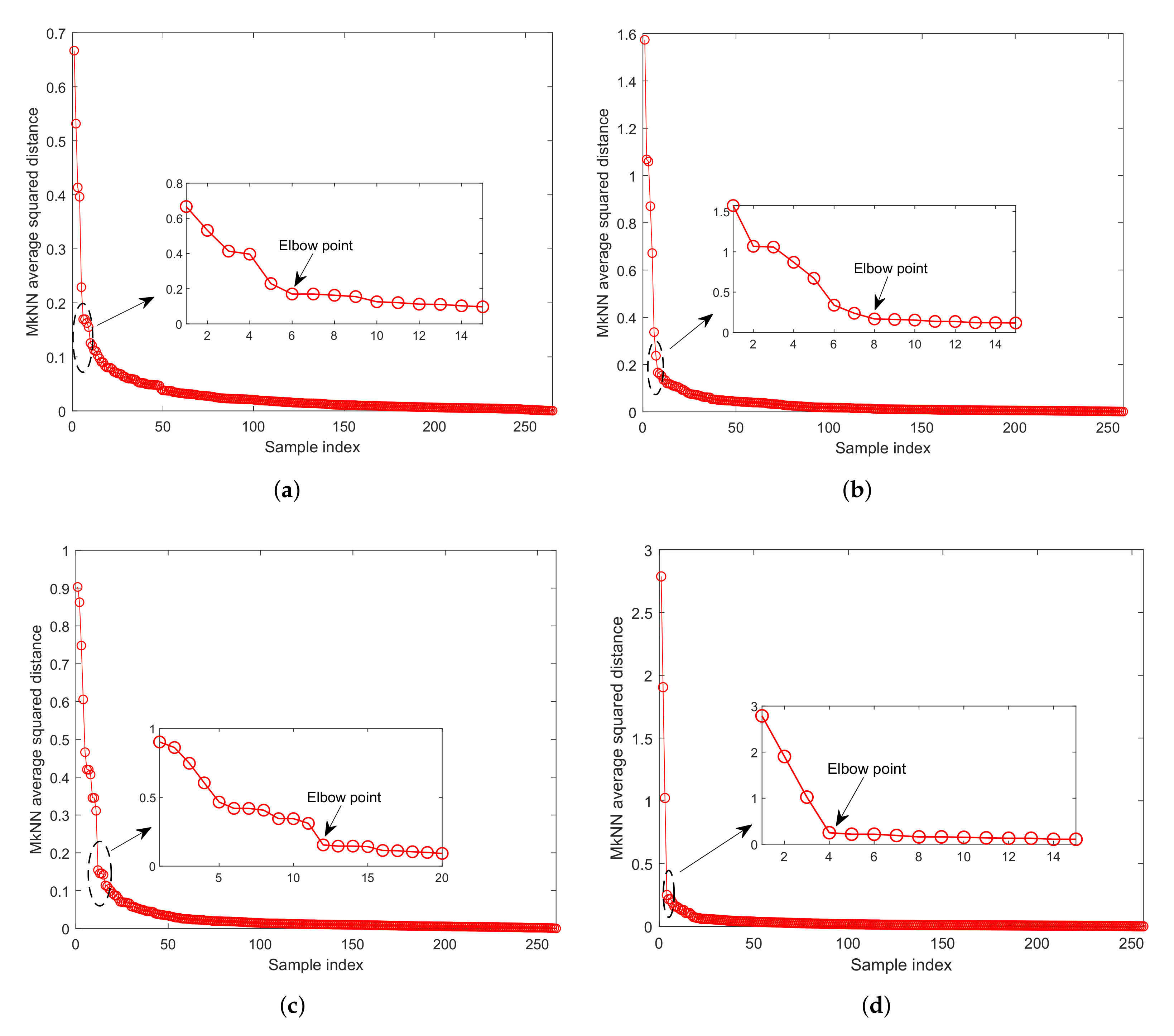
It can be observed from Figure 5 that, for outliers with mutual protection, the corresponding MkNN distance statistic is significantly larger than that of the normal training sample. Therefore, the elbow method [26] is used to eliminate outliers with mutual protection: first, arrange the MkNN distance statistics of the training samples in descending order, then determine all samples before the elbow position as outliers with mutual protection, and finally eliminate these outliers from the training set.

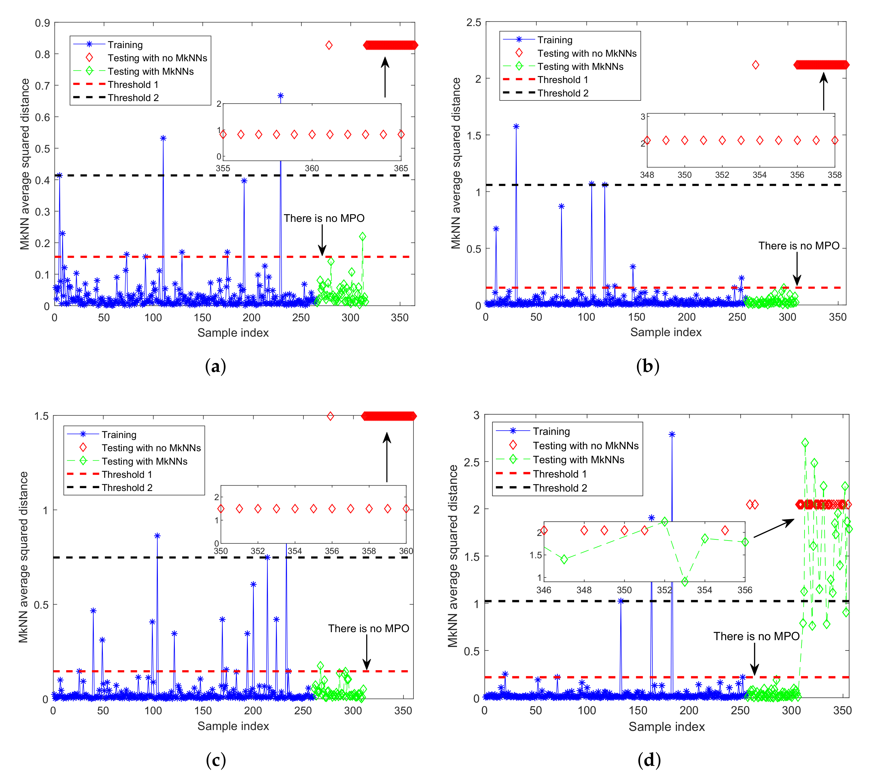
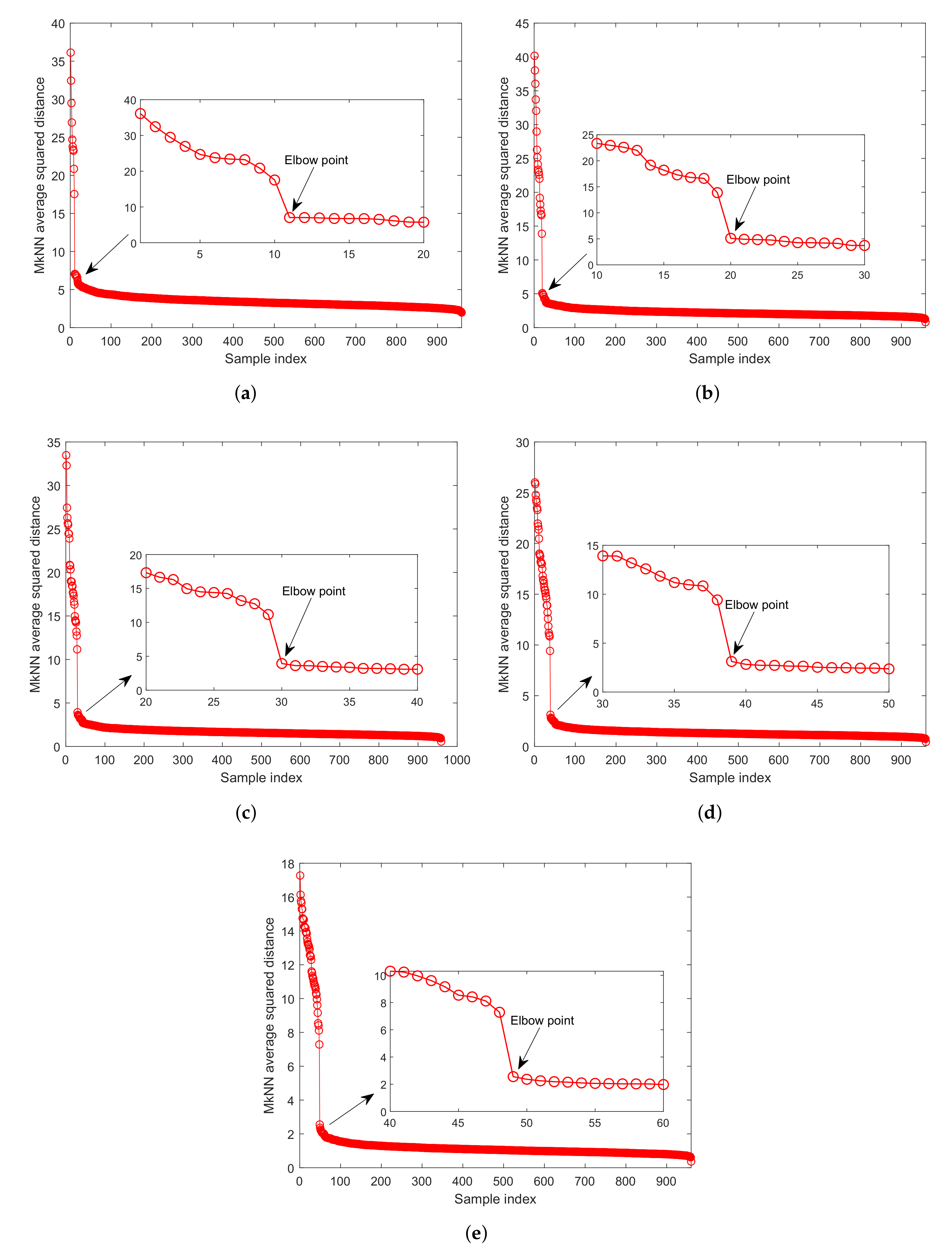
As shown in Figure 6, the outliers with mutual protection can be identified according to the elbow method, that is, all samples before the elbow point. After determining the outliers with mutual protection, these outliers need to be removed from the training set. Finally, the process monitoring method was repeated. The detection results are shown in Figure 7. After eliminating outliers with mutual protection, the recalculated threshold (that is, the red dotted line in Figure 7) is more reasonable, and the FDR has reached 100.00%, as shown in

Table 4. FDR (%) and FAR (%) of FD-MkNN of the numerical example that eliminates outliers with mutual protection phenomenon.

	2% Outliers	3% Outliers	4% Outliers	5% Outliers
FDR	100.00	100.00	100.00	100.00
FAR	4.00	2.00	4.00	4.00

.

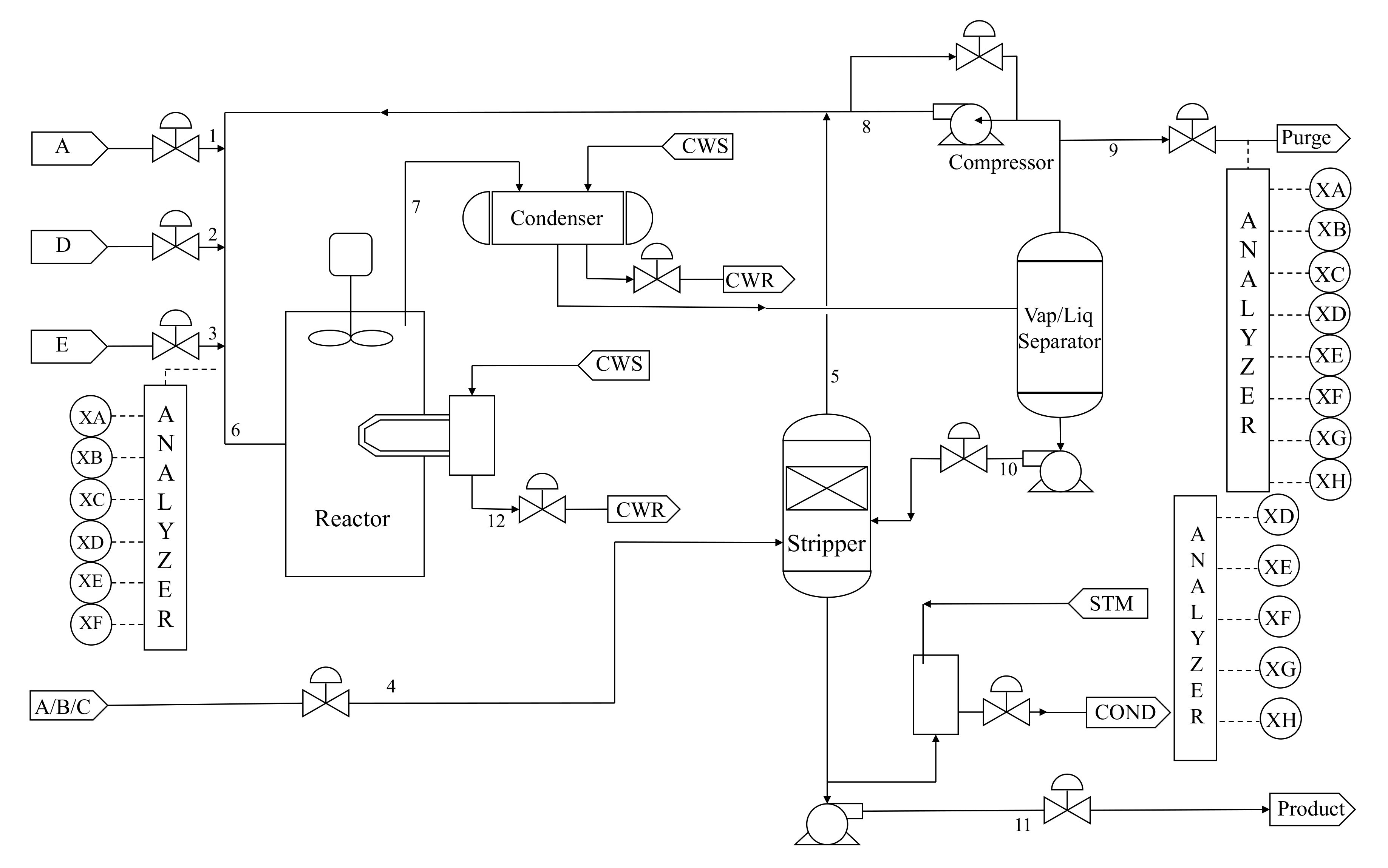
3.2. The Tennessee Eastman Process

When comparing the performance or effectiveness of process monitoring methods, the TEP [27] is a benchmark choice. In [28,29], Downs and Vogel proposed the simulation platform. There are five major operating units in the TEP, namely, a product stripper, a recycle compressor, a vapor–liquid separator, a product condenser, and a reactor. The process has four kinds of reactants (A, C, D, E), two products (G, H), contains catalyst (B), and byproducts (F). There are 11 manipulated variables (No.42–No.52), 22 process measurements (No.1–No.22), and 19 composition variables (No.23–No.41). For detailed information on the 52 monitoring variables and 21 fault patterns, see ref. [27]. The flowchart of the process is given in Figure 8.

The number of training samples and the number of validation samples are 960 and 480, respectively. In addition, there are 960 testing samples where the fault is introduced from the 161st sample. To simulate the situation that the training data contains outliers, outliers whose magnitude is twice the normal data are randomly added to the training data. The thresholds of different methods are all calculated at a confidence level of $99\%$.

These three faults are chosen to demonstrate the effectiveness of the proposed method. The parameter k of FD-kNN is 3. The parameters $k_1$ and $k_2$ of FD-MkNN are 42 and 45, respectively. For the FD-MkNN method, the outliers with mutual protection phenomenon are first eliminated by the elbow method, as shown in Figure 9.

According to [29,30], fault 1 is a step fault with a significant amplitude change. When fault 1 occurs, eight process variables are affected.

Figure 10 and Figure 11 are the monitoring results of fault 1 by FD-kNN and FD-MkNN, respectively. As the proportion of outliers increases, the detection results of kNN and MkNN for fault 1 are not significantly affected. For example, the FDR of MkNN for fault 1 remains at 99.00%, as shown in

Table 5. FDR (%) of FD-kNN and FD-MkNN for fault 1 of TEP.

Method	No Outlier	1% Outliers	2% Outliers	3% Outliers	4% Outliers	5% Outliers
FD-kNN	99.50	98.75	98.50	98.75	98.50	98.50
FD-MkNN	99.50	99.00	99.00	99.00	99.00	99.00

. Because fault 1 is a step fault with a significant amplitude change, the outliers introduced in this experiment are insignificant in the face of this fault. Although these outliers also deviate the control limits from normal levels, they do not have much impact on the fault detection phase. The fault false alarm rate of FD-kNN and FD-MkNN is shown in

Table 6. FAR (%) of FD-kNN and FD-MkNN for fault 1 of TEP.

Method	No Outlier	1% Outliers	2% Outliers	3% Outliers	4% Outliers	5% Outliers
FD-kNN	0.63	0.00	0.00	0.00	0.00	0.00
FD-MkNN	0.63	0.00	0.00	0.00	0.00	0.00

.

The fault 7 is also a step fault, but its magnitude changes are small, and only one process variable (i.e., variable 45) is affected.

Figure 12 and Figure 13 are the monitoring results of fault 7 by FD-kNN and FD-MkNN, respectively. As shown in

Table 7. FDR (%) of FD-kNN and FD-MkNN for fault 7 of TEP.

Method	No Outlier	1% Outliers	2% Outliers	3% Outliers	4% Outliers	5% Outliers
FD-kNN	100.00	79.75	25.25	25.25	20.38	18.75
FD-MkNN	100.00	99.63	97.63	94.75	93.63	92.75

, as the proportion of outliers increases, the FDR of FD-kNN drops from 100.00% to 18.75%, while the FDR of FD-MkNN does not decrease significantly and remains above 90.00%. The fault false alarm rate of FD-kNN and FD-MkNN is shown in

Table 8. FAR (%) of FD-kNN and FD-MkNN for fault 7 of TEP.

Method	No Outlier	1% Outliers	2% Outliers	3% Outliers	4% Outliers	5% Outliers
FD-kNN	0.00	0.00	0.00	0.00	0.00	0.00
FD-MkNN	0.00	0.00	0.00	0.00	0.00	0.00

.

According to the detection results of fault 1 and fault 7, it can be seen that FD-MkNN is suitable for the processing of incipient faults. Because outliers will significantly increase the threshold, the detection statistic of incipient faults is lower than the threshold. The proposed method eliminates outliers by judging whether the samples have MkNNs, thereby improving the fault detection performance.

Fault 13 is a slow drift in the reaction kinetics. Figure 14 and Figure 15 are the monitoring results of fault 13 by FD-kNN and FD-MkNN, respectively. In

Table 9. FDR (%) of FD-kNN and FD-MkNN for fault 13 of TEP.

Method	No Outlier	1% Outliers	2% Outliers	3% Outliers	4% Outliers	5% Outliers
FD-kNN	95.38	90.50	84.88	85.00	82.25	80.25
FD-MkNN	95.38	92.75	91.88	91.63	91.75	92.00

and

Table 10. FAR (%) of FD-kNN and FD-MkNN for fault 13 of TEP.

Method	No Outlier	1% Outliers	2% Outliers	3% Outliers	4% Outliers	5% Outliers
FD-kNN	1.25	0.00	0.00	0.00	0.00	0.00
FD-MkNN	1.25	0.63	0.63	0.63	0.63	0.63

, as the proportion of outliers increases, the FDR of the FD-MkNN is always better than that of FD-kNN, while the FAR is higher than that of kNN. Due to the appearance of outliers, the threshold of the kNN is increased so the FAR of FD-kNN is always 0.00%.

4. Discussion

The neighbors of the samples found by kNN on a data set containing outliers may not be true neighbors, but a kind of pseudo neighbor. If such pseudo-nearest neighbors are used to calculate the threshold, the threshold or control limit will deviate significantly from the normal level, thereby degrading the fault detection performance.

The MkNN method determines outliers through checking whether the samples have MkNNs, which simultaneously realizes the elimination of outliers and the fault detection by using the same rule. Through the detection of fault 1 and fault 7 in the TEP, it can be seen that the FD-MkNN has obvious advantages for detecting incipient faults because the incipient faults are more sensitive to outliers.

This work stresses the superiority and promise of the MkNN rule for fault detection, especially for industrial processes with outliers. The MkNN-method-based fault isolation or diagnosis part is currently underway.

5. Conclusions

In this paper, a novel fault detection approach based on the mutual k-nearest neighbor method is proposed. The primary characteristic of our method is that the calculation of the distance statistics for fault detection uses the MkNN rule instead of kNN. The proposed method simultaneously realizes the elimination of outliers and the fault detection using Mutual kNN rule. Specifically, before the training phase, part of the outliers in the training samples are removed so that the outliers will not affect the determination of the control limit in the training phase; in the fault detection phase, MkNN carries more valuable and reliable information than kNN. Furthermore, the effect of PNN is eliminated. Furthermore, the mutual protection problem of outliers is solved using the elbow rule, which improves the performance of fault detection. The experiments on numerical examples and TEP verify the effectiveness of the proposed method.

The proposed FD-MkNN can be seen as an alternative method in monitoring the industrial processes with outliers. In addition, the MkNN method based fault isolation or diagnosis part is currently underway.

References

- Chiang, L.H.; Russell, E.L.; Braatz, R.D. Fault Detection and Diagnosis in Industrial Systems; Springer: London, UK, 2001. [Google Scholar] [CrossRef]
- Arunthavanathan, R.; Khan, F.; Ahmed, S.; Imtiaz, S. An analysis of process fault diagnosis methods from safety perspectives. Comput. Chem. Eng. 2021, 145, 107197. [Google Scholar] [CrossRef]
- Zhao, S.; Zhang, J.; Xu, Y. Monitoring of processes with multiple operating modes through multiple principle component analysis models. Ind. Eng. Chem. Res. 2004, 43, 7025–7035. [Google Scholar] [CrossRef]
- Fezai, R.; Mansouri, M.; Okba, T.; Harkat, M.F.; Bouguila, N. Online reduced kernel principal component analysis for process monitoring. J. Process Control 2018, 61, 1–11. [Google Scholar] [CrossRef]
- Peres, F.; Peres, T.N.; Fogliatto, F.S.; Anzanello, M.J. Fault detection in batch processes through variable selection integrated to multiway principal component analysis. J. Process Control 2019, 80, 223–234. [Google Scholar] [CrossRef]
- Deng, X.G.; Lei, W. Modified kernel principal component analysis using double-weighted local outlier factor and its application to nonlinear process monitoring. ISA Trans. 2017, 72, 218–228. [Google Scholar] [CrossRef]
- Wang, J.; He, Q.P. Multivariate statistical process monitoring based on statistics pattern analysis. Ind. Eng. Chem. Res. 2010, 49, 7858–7869. [Google Scholar] [CrossRef]
- Zhou, Z.; Wen, C.L.; Yang, C.J. Fault Isolation Based on k-Nearest Neighbor Rule for Industrial Processes. IEEE Trans. Ind. Electron. 2016, 63, 2578–2586. [Google Scholar] [CrossRef]
- Zhou, Z.; Li, Z.X.; Cai, Z.D.; Wang, P.L. Fault Identification Using Fast k-Nearest Neighbor Reconstruction. Processes 2019, 7, 340. [Google Scholar] [CrossRef] [Green Version]
- Qin, S.J. Survey on data-driven industrial process monitoring and diagnosis. Annu. Rev. Control 2012, 36, 220–234. [Google Scholar] [CrossRef]
- He, Q.P.; Wang, J. Fault detection using the k-nearest neighbor rule for semiconductor manufacturing processes. IEEE Trans. Semicond. Manuf. 2007, 20, 345–354. [Google Scholar] [CrossRef]
- Nomikos, P.; Macgregor, J.F. Monitoring Batch Process Using Multiway Principal Componet Analysis. AIChE J. 1994, 40, 1361–1375. [Google Scholar] [CrossRef]
- Ku, W.; Storer, R.H.; Georgakis, C. Disturbance detection and isolation by dynamic principal component analysis. Chemom. Intell. Lab. Syst. 1995, 30, 179–196. [Google Scholar] [CrossRef]
- Lee, J.M.; Yoo, C.K.; Choi, S.W.; Vanrolleghem, P.A.; Lee, I.B. Nonlinear process monitoring using kernel principal component analysis. Chem. Eng. Sci. 2004, 59, 223–234. [Google Scholar] [CrossRef]
- Lee, J.M.; Yoo, C.K.; Lee, I.B. Fault detection of batch processes using multiway kernel principal component analysis. Comput. Chem. Eng. 2004, 28, 1837–1847. [Google Scholar] [CrossRef]
- Sang, W.C.; Lee, C.; Lee, J.M.; Jin, H.P.; Lee, I.B. Fault detection and identification of nonlinear processes based on kernel pca. Chemom. Intell. Lab. Syst. 2005, 75, 55–67. [Google Scholar] [CrossRef]
- Zhang, Y.; Wu, X. Integrating induction and deduction for noisy data mining. Inf. Sci. 2010, 180, 2663–2673. [Google Scholar] [CrossRef]
- Liu, H.; Zhang, S. Noisy data elimination using mutual k-nearest neighbor for classification mining. J. Syst. Softw. 2012, 85, 1067–1074. [Google Scholar] [CrossRef]
- Barnett, V.; Lewis, T. Outliers in Statistical Data; Wiley: Hoboken, NJ, USA, 1974. [Google Scholar] [CrossRef]
- Zhu, J.L.; Ge, Z.Q.; Song, Z.H.; Gao, F.R. Review and big data perspectives on robust data mining approaches for industrial process modeling with outliers and missing data. Annu. Rev. Control 2018, 46, 107–133. [Google Scholar] [CrossRef]
- Brighton, H.; Mellish, C. Advances in Instance Selection for Instance-Based Learning Algorithms. Data Min. Knowl. Discov. 2002, 6, 153–172. [Google Scholar] [CrossRef]
- He, Q.P.; Wang, J. Statistics Pattern Analysis: A New Process Monitoring Framework and its Application to Semiconductor Batch Processes. AIChE J. 2011, 57, 107–121. [Google Scholar] [CrossRef]
- Verdier, G.; Ferreira, A. Adaptive mahalanobis distance and k-nearest neighbor rule for fault detection in semiconductor manufacturing. IEEE Trans. Semicond. Manuf. 2011, 24, 59–68. [Google Scholar] [CrossRef]
- Ding, C.; Chris, H.Q.; He, X.F. K-nearest-neighbor consistency in data clustering: Incorporating local information into global optimization. In Proceedings of the 2004 ACM Symposium on Applied Computing, Nicosia, Cyprus, 14–17 March 2004. [Google Scholar] [CrossRef]
- Zhu, J.L.; Ge, Z.Q.; Song, Z.H. Robust supervised probabilistic principal component analysis model for soft sensing of key process variables. Chem. Eng. Sci. 2015, 122, 573–584. [Google Scholar] [CrossRef]
- Liu, F.; Deng, Y. Determine the number of unknown targets in Open World based on Elbow method. IEEE Trans. Fuzzy Syst. 2020, 29, 986–995. [Google Scholar] [CrossRef]
- Ricker, N.L. Optimal steady-state operation of the Tennessee Eastman challenge process. Comput. Chem. Eng. 1995, 19, 949–959. [Google Scholar] [CrossRef]
- Downs, J.J.; Vogel, E.F. A plant-wide industrial process control problem. Comput. Chem. Eng. 1993, 17, 245–255. [Google Scholar] [CrossRef]
- Russell, E.L.; Chiang, L.H.; Braatz, R.D. Data-Driven Techniques for Fault Detection and Diagnosis in Chemical Processes; Springer: London, UK, 2000. [Google Scholar] [CrossRef]
- Liu, J. Fault diagnosis using contribution plots without smearing effect on non-faulty variables. J. Process Control 2012, 22, 1609–1623. [Google Scholar] [CrossRef]
Publisher’s Note: MDPI stays neutral with regard to jurisdictional claims in published maps and institutional affiliations. |
© 2022 by the authors. Licensee MDPI, Basel, Switzerland. This article is an open access article distributed under the terms and conditions of the Creative Commons Attribution (CC BY) license (https://creativecommons.org/licenses/by/4.0/).