Closed-Form Valuation of Discounted Cash Flows with Finite Poisson Arrivals in a Finite Horizon

Abstract

This paper derives a closed-form expression for the expected discounted value of aggregate cash flows when arrival times follow a Poisson process but both the time horizon and the number of arrivals are finite. The result provides a tractable analytical formula for the expected discounted sum under simultaneous constraints on time and arrival counts. We show that the expression converges to the well-known infinite-horizon and infinite-arrival results as limiting cases. Numerical illustrations demonstrate the behavior of the formula under different parameter values. The result can be interpreted as the valuation of a discounted compound Poisson process with finite constraints and may be useful in stochastic modeling and risk-analysis applications. The proposed formula provides a simple analytical tool for evaluating discounted losses or revenues in finite risk portfolios.

1. Introduction

The valuation of discounted cash flows subject to random arrival times is a fundamental problem in quantitative finance and actuarial science. This problem is traditionally modeled using compound Poisson processes, where the focus often lies on infinite horizons or asymptotic behaviors. Compound Poisson processes are widely used to describe aggregate losses in risk modeling and actuarial applications; see, for example, Embrechts et al. (1997) and Klugman et al. (2012). Extensive literature exists on the distributional properties of discounted compound sums. For instance, Gjessing and Paulsen (1997) and Paulsen (1997) analyze present value distributions with applications to ruin theory, while Zhang (2019) provides a comprehensive review of discounted compound Poisson sums under general distributions.

While these studies offer mathematically general results, their solutions often involve complex integral equations or recursive formulations that can be computationally intensive for practitioners. More specifically, existing works that incorporate finite-horizon constraints often rely on numerical inversion of Laplace transforms or recursive approximations, whereas finite-arrival formulations are more commonly studied under infinite-horizon settings. Explicit formulas for the joint case of finite horizon and finite arrivals are not usually available in a simple analytical form, because this combination leads to truncated integrals, such as expressions involving incomplete Gamma functions, that are often left in recursive or integral form rather than reduced to a practically usable closed-form expression. Furthermore, while finite-horizon valuation issues are central in insurance applications (e.g., van den Broek 2014), simple exact closed-form expressions for the expected discounted sum are not commonly provided.

In practical applications, however, decision-makers frequently encounter scenarios constrained by both a finite time horizon and a finite maximum number of events. In the context of finance, for example, existing studies often focus on the pricing of bonds subject to the default risk of a single firm (e.g., van den Broek 2014; Wüthrich 2011). However, banks must manage credit risk for a portfolio of N loans over a specific T-year period. Similarly, in revenue management, standard inventory models using compound Poisson demands (e.g., Feeney and Sherbrooke 1966; Schlosser 2016) often assume infinite horizons, whereas actual sales events are strictly limited by time and stock. In such cases, general asymptotic results are insufficient, and a simple, explicit formula is preferred.

The objective of this paper is to derive a closed-form expression for the expected discounted sum of a compound Poisson process when both the time horizon and the number of arrivals are finite. To the best of our knowledge, explicit formulas for this finite-horizon and finite-arrival setting have not been previously documented in closed form. Specifically, we examine the following value $V_N\left(T\right)$:

$$\begin{array}{c}\hfill V_N\left(T\right):=\mathbb{E}\left[\sum _{n=1}^N{\mathrm{e}}^{-\rho X_n}{Z}_n{\mathbf{1}}_{\{X_n<T\}}\right],\end{array}$$

(1)

where $X_n$ is the n-th random arrival time, $Z_n$ is the stochastic cash flow size, $\rho >0$ is the discount rate, and ${\mathbf{1}}_A$ denotes the indicator function of a measurable set A. By imposing a specific yet practical assumption on the cash flows—that they are independent and identically distributed with a constant mean—we successfully derive a tractable closed-form solution (Theorem 1). Unlike infinite-horizon approximations, our finite-horizon formula can generate economically non-negligible deviations even for moderate values of N and T, highlighting the importance of explicitly accounting for finite constraints.

In particular, relying on infinite-horizon or infinite-arrival approximations may lead to non-negligible deviations in valuation when finite constraints are present. For example, when evaluating the default risk of a finite portfolio of 10 firms, an infinite-arrival approximation effectively ignores the cap on the number of possible defaults and may therefore overestimate the expected total discounted loss. This illustrates the practical importance of explicitly accounting for finite constraints.

Our approach offers direct applicability to various fields. One possible interpretation is the cumulative loss from defaults in a portfolio of N firms where default intensities are assumed independent (a baseline model for credit risk). In sports economics, it evaluates the financial risk of player injuries during a fixed-term contract (e.g., Kudo et al. 2024; Tunaru et al. 2005), where $Z_n$ represents the value depreciation due to the n-th injury. In revenue management, it applies to inventory liquidation or limited-time sales events (e.g., “drops” in the fashion industry) where customer orders arrive randomly but inventory is limited.

The main contribution of this paper is the derivation of a practically useful closed-form formula for the finite-horizon, finite-arrival setting, which has received less attention than infinite-horizon models. In addition, as a validation of the mathematical consistency of the framework, we show that the proposed formula converges to standard infinite-horizon valuations as asymptotic special cases. This supports the interpretation of our model as a consistent bridge between finite practical constraints and general theoretical foundations.

From a stochastic-process perspective, the model corresponds to a discounted compound Poisson process under simultaneous constraints on the time horizon and the number of arrivals. While infinite-horizon approximations are often used for analytical convenience, finite constraints naturally arise in many practical settings where both the observation window and the number of events are limited. The present result provides a tractable analytical expression for such finite systems.

The remainder of this paper is organized as follows. Section 2 describes the model and derives the explicit solutions. Section 3 presents numerical sensitivity analyses and practical implications. Section 4 concludes this paper.

2. Model

2.1. Preliminaries

We consider the expected total discounted cash flow with Poisson arrivals over a finite horizon T. The n-th Poisson arrival time is denoted by $X_n$ and the cash flow at time $X_n$ by $Z_n$ where $n\in \mathbb{N}$. Then, ${\left\{X_n\right\}}_{n=1}^{\infty }$ denotes the sequence of arrival times, and it satisfies

$$\begin{array}{c}\hfill 0<X_1<\cdots <X_n<\cdots .\end{array}$$

The two sequences, ${\left\{X_n\right\}}_{n=1}^{\infty }$ and ${\left\{Z_n\right\}}_{n=1}^{\infty }$, are defined on a filtered probability space $(\mathsf{\Omega },\mathcal{F},{\left\{{\mathcal{F}}_t\right\}}_{t\ge 0},\mathbb{P})$, where ${\left\{{\mathcal{F}}_t\right\}}_{t\ge 0}$ is the filtration generated by

$${\mathcal{F}}_t:=\sigma ({\left\{X_n\right\}}_{n=1,2,\dots ,k:X_k\le t<X_{k+1}},{\left\{Z_n\right\}}_{n=1,2,\dots ,k}).$$

Assumption 1.

We assume ${\left\{Z_n\right\}}_{n=1}^{\infty }$ are positive i.i.d. random variables independent of ${\left\{X_n\right\}}_{n=1}^{\infty }$, and the expected value of $Z_n$ exists:

$$\begin{array}{cc}\hfill \mathbb{E}\left[Z_n\right]& =\mu >0.\hfill \end{array}$$

Under Assumption 1, (1) can be written as

$$\begin{array}{cc}\hfill V_N\left(T\right)& =\mathbb{E}\left[\sum _{n=1}^N{\mathrm{e}}^{-\rho X_n}{\mathbf{1}}_{\{X_n<T\}}\right]\mu ,\hfill \end{array}$$

(2)

which we will calculate in Section 2.2.

The definitions of the discount function and the total discount function help us to calculate (2).

Definition 1.

We define the discount function $d_n\left(T\right)$ for the n-th arrival and the total discount function $D_N\left(T\right)$ for N arrivals over a finite horizon $[0,T]$ as follows:

$$\begin{array}{cc}\hfill d_n\left(T\right)& :=\mathbb{E}\left[{\mathrm{e}}^{-\rho X_n}{\mathbf{1}}_{\{X_n<T\}}\right],\hfill \\ \hfill D_N\left(T\right)& :=\sum _{n=1}^N{d}_n\left(T\right)=\mathbb{E}\left[\sum _{n=1}^N{\mathrm{e}}^{-\rho X_n}{\mathbf{1}}_{\{X_n<T\}}\right].\hfill \end{array}$$

From Definition 1, we can rewrite (2) as

$$\begin{array}{c}\hfill V_N\left(T\right)=D_N\left(T\right)\mu .\end{array}$$

(3)

Therefore, the analysis of $V_N\left(T\right)$ is equivalent to that of $D_N\left(T\right)$.

Before proceeding to the analysis of $D_N\left(T\right)$, we recall that under the standard Poisson arrival assumption with rate $\lambda$, the inter-arrival times are independent and exponentially distributed. Consequently, the n-th arrival time $X_n$ follows an Erlang distribution with parameters n and $\lambda$, denoted as

$$\begin{array}{c}\hfill X_n\sim \mathrm{Erlang}(n,\lambda ).\end{array}$$

2.2. Analytical Solutions

The following theorem gives our main result, namely, a closed-form expression for the expected total discounted cash flow when both the horizon T and the number of Poisson arrivals N are finite.

Theorem 1.

The expected total discounted cash flow with finite arrivals over a finite horizon $[0,T]$, $V_N\left(T\right)$, is given by (3), and

$$\begin{array}{cc}\hfill D_N\left(T\right)& ={\displaystyle \frac{\lambda }{\rho }}\left(1-{\left({\displaystyle \frac{\lambda }{\rho +\lambda }}\right)}^{N}F(T;N,\rho +\lambda )-{\mathrm{e}}^{-\rho T}\overline{F}(T;N,\lambda )\right),\hfill \end{array}$$

(4)

where $F(x;n,\lambda )$ denotes the cumulative distribution function of $X_n$, and $\overline{F}(x;n,\lambda ):=1-F(x;n,\lambda )$ is the survival function for $X_n$.

From the relationship between Erlang and Poisson distributions, $F(x;n,\lambda )$ represents the probability of observing at least n arrivals over $[0,x]$:

$$\begin{array}{c}\hfill F(x;n,\lambda )=1-\sum _{k=0}^{n-1}{\displaystyle \frac{{\left(\lambda x\right)}^k}{k!}}{\mathrm{e}}^{-\lambda x}.\end{array}$$

A close examination of (4) reveals that our closed-form solution for the case of finite arrivals over a finite horizon consistently converges to well-known results for both the infinite arrival and the perpetual cases, which is summarized in the following corollary. The proofs are provided in Appendix A.

Corollary 1.

We have the following results for limiting values:

$$\begin{array}{cc}\hfill \underset{N\to \infty }{lim}{D}_N\left(T\right)& =:D_{\infty }\left(T\right)=\mathbb{E}\left[\sum _{n=1}^{\infty }{\mathrm{e}}^{-\rho X_n}{\mathbf{1}}_{\{X_n<T\}}\right]={\displaystyle \frac{\lambda }{\rho }}\left(1-{\mathrm{e}}^{-\rho T}\right),\hfill \\ \hfill \underset{T\to \infty }{lim}{D}_N\left(T\right)& =:D_N(\infty )=\mathbb{E}\left[\sum _{n=1}^N{\mathrm{e}}^{-\rho X_n}\right]={\displaystyle \frac{\lambda }{\rho }}\left(1-{\left({\displaystyle \frac{\lambda }{\rho +\lambda }}\right)}^N\right),\hfill \\ \hfill \underset{N,T\to \infty }{lim}{D}_N\left(T\right)& =:D_{\infty }(\infty )=\mathbb{E}\left[\sum _{n=1}^{\infty }{\mathrm{e}}^{-\rho X_n}\right]={\displaystyle \frac{\lambda }{\rho }}.\hfill \end{array}$$

Note that $D_N\left(T\right)$ reflects the influence of a finite horizon on $D_N(\infty )$, as well as the effect of finite arrivals within a finite horizon on $D_{\infty }(\infty )$.

3. Numerical Examples and Practical Implications

3.1. Sensitivity Analysis

This section examines how the key parameters—the discount rate $\rho$, arrival rate $\lambda$, maximum number of arrivals N, and maturity T—affect the expected total discounted cash flow $V_N\left(T\right)$. The benchmark parameter values are set to $\rho =0.2$, $\lambda =0.5$, $N=10$, and $T=10$. Through this section, we set $\mu =1$ without loss of generality.

Table 1. Sensitivity analysis for problem parameters under finite horizons and finite arrivals.

$\mathit{\rho }$	$\mathit{\lambda }$	N	T	${\mathit{V}}_{\mathit{N}}\left(\mathit{T}\right)$
0.1	0.5	10	10	3.151
0.2	0.5	10	10	2.158
0.3	0.5	10	10	1.582
0.2	0.4	10	10	1.729
0.2	0.5	10	10	2.158
0.2	0.6	10	10	2.580
0.2	0.5	11	10	0.714
0.2	0.5	13	10	1.574
0.2	0.5	15	10	1.967
0.2	0.5	10	10	2.158
0.2	0.5	∞	10	2.162
0.2	0.5	10	11	0.453
0.2	0.5	10	13	1.128
0.2	0.5	10	15	1.580
0.2	0.5	10	10	2.158
0.2	0.5	10	∞	2.414

Note: The values of $V_N\left(T\right)$ in this table are rounded to the third decimal place.

reports the sensitivity of $V_N\left(T\right)$ with respect to each parameter. The results are consistent with economic intuition. An increase in the arrival rate $\lambda$, the number of arrivals N, or the maturity T leads to a higher expected discounted value, while a higher discount rate $\rho$ reduces the value. These monotonic relationships directly follow from the closed-form expression derived in Theorem 1.

From a revenue management perspective, a higher arrival rate corresponds to more frequent customer orders, increasing expected revenue. Conversely, when cash flows represent losses, such as defaults or injuries, the same comparative statics characterize the expected cumulative loss. Importantly, the closed-form solution allows these effects to be quantified transparently without numerical recursion or simulation. In particular, comparing $V_N\left(T\right)$ with its infinite-arrival counterpart $V_{\infty }\left(T\right)$ reveals that the infinite approximation may substantially overestimate expected values when both the horizon and the number of arrivals are finite. For the benchmark parameter set $(\rho ,\lambda ,N,T)=(0.2,0.5,10,10)$, the corresponding infinite-arrival and infinite-horizon benchmark values are $V_{\infty }\left(T\right)=2.162$ and $V_N(\infty )=2.414$, respectively, compared with the finite constrained value $V_N\left(T\right)=2.158$. This indicates that, in this baseline case, the finite-horizon constraint has a much larger impact on valuation than the finite-arrival cap.

3.2. Application to Credit Risk Portfolio Management

We illustrate the practical relevance of our framework using a simple credit risk setting, where the objective is not empirical calibration but to provide a transparent baseline for finite-horizon portfolio risk assessment. Consider a bank managing a finite portfolio of N firms over a finite risk horizon T. Each firm is subject to default risk, and default times are assumed to be independent and exponentially distributed with intensity $\lambda$, which serves as a baseline model in credit risk analysis. While corporate defaults are known to exhibit correlation during systemic events such as the Global Financial Crisis, the present framework is intended to provide a transparent baseline under the standard independence assumption, against which more complex dependence structures can be assessed.

The relationship between the one-year cumulative default probability and the default intensity is given by

$$\begin{array}{c}\hfill \mathbb{P}(\tau \le 1)=1-{\mathrm{e}}^{-\lambda },\end{array}$$

allowing default intensities to be inferred directly from observed default probabilities.

Table 2. One-year cumulative default probabilities and the corresponding default intensity for credit ratings BB, B, and CCC/C.

Rating	ℙ(τ ≤ 1)	$\mathit{\lambda }$
BB	02.99%	0.0132
B	21.95%	0.1076
CCC/C	53.85%	0.3358

reports one-year cumulative default probabilities for Japanese firms with credit ratings BB, B, and CCC/C reported by JCR (2024), together with the corresponding default intensities.

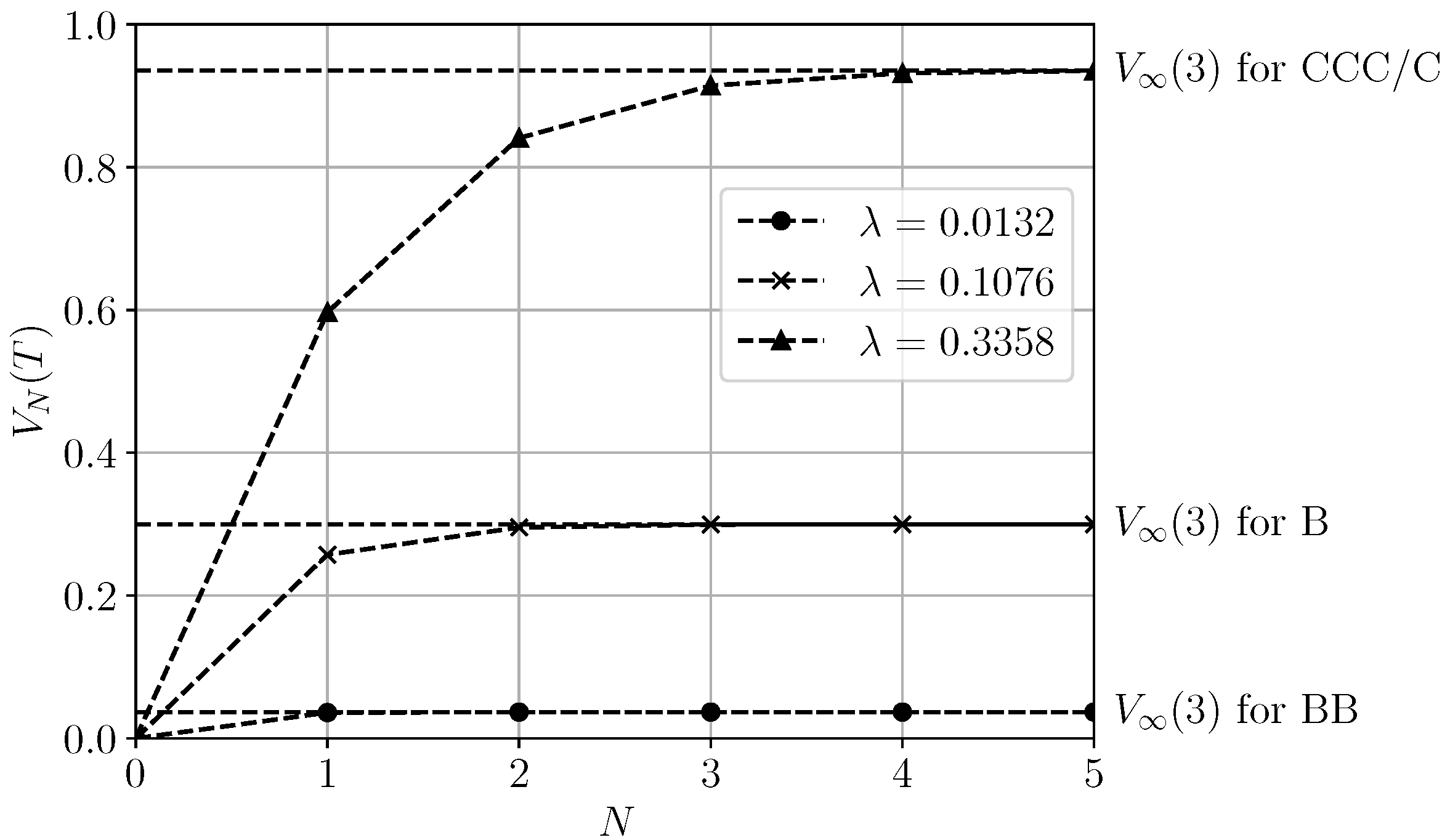
Figure 1 plots the expected total discounted loss $V_N\left(T\right)$ for each rating category under illustrative parameter values $\rho =0.05$ and $T=3$. As the number of firms increases, $V_N\left(T\right)$ converges to its limiting value $V_{\infty }\left(T\right)$. Beyond a certain portfolio size—referred to as the threshold number—adding more firms does not increase the expected total discounted loss. This threshold is smallest for low-risk firms (BB) and largest for high-risk firms (CCC/C), reflecting their higher default intensities.

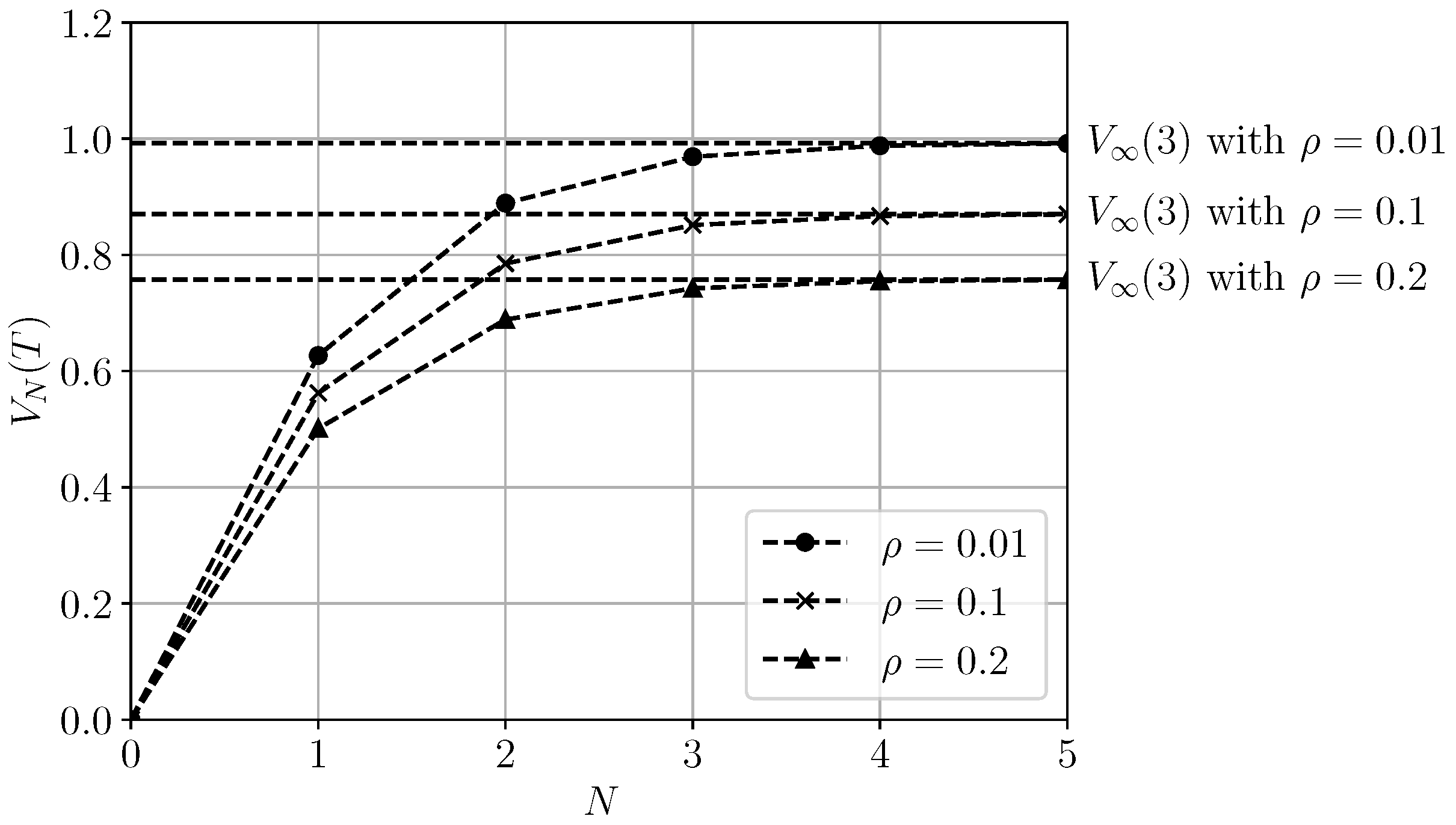
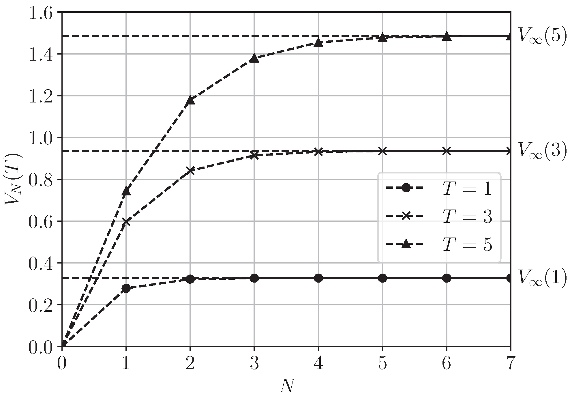
Figure 2 and Figure 3 further explore the effects of the discount rate and maturity for the CCC/C rating. Figure 2 shows that changes in the discount rate have little impact on the threshold number in this setting, as the relatively high default intensity dominates the convergence speed. In contrast, Figure 3 demonstrates that the threshold number increases with maturity T, indicating that longer risk horizons amplify the impact of finite arrivals.

From a practical perspective, the threshold number can be interpreted as a decision-relevant benchmark. Beyond this level, expanding the portfolio size does not materially change expected discounted losses, implying that additional risk aggregation yields diminishing informational value. This suggests that, for portfolios exceeding the threshold size, monitoring aggregate expected losses may be sufficient without tracking marginal additions individually. The explicit closed-form formula in Theorem 1 enables practitioners to identify such thresholds analytically, providing a simple and transparent tool for finite-horizon portfolio risk assessment.

As a practical rule of thumb, the threshold portfolio size may be expected to increase with the mean number of arrivals over the horizon, $\lambda T$. Since the number of arrivals over $[0,T]$ follows a Poisson distribution with mean and variance $\lambda T$, a rough benchmark for the threshold may be obtained by considering an upper-tail coverage level such as $\lambda T+3\sqrt{\lambda T}$. This heuristic is only intended as an intuitive guide, since the effective threshold also depends on discounting and on the tolerance used to judge proximity to the asymptotic benchmark.

4. Conclusions

This paper derives an explicit closed-form formula for the expected total discounted cash flow under finite-horizon and finite-arrival constraints. The resulting tractable expression provides a transparent baseline for evaluating threshold effects in finite portfolios and for practical risk-management applications. While the current framework relies on the standard assumption of homogeneous Poisson arrivals and independent events, future research could extend the methodology in several directions. In particular, allowing for non-homogeneous Poisson arrivals with time-varying intensities or introducing dependence structures to capture correlated defaults during systemic crises would further enhance the practical robustness of the framework.