A Machine Learning-Based Calibration Framework for Low-Cost PM_2.5 Sensors Integrating Meteorological Predictors

Abstract

Low-cost sensors (LCSs) have rapidly expanded in urban air quality monitoring but still suffer from limited data accuracy and vulnerability to environmental interference compared with regulatory monitoring stations. To improve their reliability, we proposed a machine learning (ML)-based framework for LCS correction that integrates various meteorological factors at observation sites. Taking Tongshan District of Xuzhou City as an example, this study carried out continuous co-location data collection of hourly PM_2.5 measurements by placing our LCS (American Temtop M10+ series) close to a regular fixed monitoring station. A mathematical model was developed to regress the PM_2.5 deviations (PM_2.5 concentrations at the fixed station—PM_2.5 concentrations at the LCS) and the most important predictor variables. The data calibration was carried out based on six kinds of ML algorithms: random forest (RF), support vector regression (SVR), long short-term memory network (LSTM), decision tree regression (DTR), Gated Recurrent Unit (GRU), and Bidirectional LSTM (BiLSTM), and the final model was selected from them with the optimal performance. The performance of calibration was then evaluated by a testing dataset generated in a bootstrap fashion with ten time repetitions. The results show that RF achieved the best overall accuracy, with R² of 0.99 (training), 0.94 (validation), and 0.94 (testing), followed by DTR, BiLSTM, and GRU, which also showed strong predictive capabilities. In contrast, LSTM and SVR produced lower accuracy with larger errors under the limited data conditions. The results demonstrate that tree-based and advanced deep learning models can effectively capture the complex nonlinear relationships influencing LCS performance. The proposed framework exhibits high scalability and transferability, allowing its application to different LCS types and regions. This study advances the development of innovative techniques that enhance air quality assessment and support environmental research.

1. Introduction

Air pollution, as one of the most pressing environmental challenges worldwide, has long attracted extensive attention from both the scientific community and the public [1,2]. Numerous studies have demonstrated that air pollution not only disrupts ecosystems but also poses serious threats to human health, with fine particulate matter (PM_2.5) being closely associated with a range of respiratory and cardiovascular diseases [3,4,5,6]. To accurately assess air quality conditions and develop effective pollution control strategies, air pollution monitoring has traditionally relied on fixed monitoring stations deployed in urban and surrounding areas over the past decades [7,8]. These stations offer high measurement accuracy and reliable data; however, their high construction and maintenance costs significantly limit their large-scale and high-density deployment [9]. In recent years, with rapid advances in sensor technology and the Internet of Things (IoT), low-cost sensors (LCS) have been increasingly adopted in air pollution monitoring. Compared with conventional fixed-site monitoring, LCS devices feature compact size, low cost, and flexible deployment, enabling large-scale and high spatiotemporal resolution observations across diverse urban settings [10,11,12]. As a result, they serve as a valuable complement to traditional monitoring networks and provide new opportunities for characterizing the spatiotemporal distribution of air pollution and supporting more refined air quality management [9,12,13].

Despite the promising prospects of LCS in air pollution monitoring, their widespread deployment and application are still hindered by a critical challenge: the relatively low quality of their measurement data [14]. Compared with regular fixed-site monitoring, LCS devices typically utilize inexpensive sensing components, resulting in lower measurement accuracy, stability, and long-term reliability. Their performance is highly susceptible to various external influences, including environmental conditions, sensor aging, and hardware variability, all of which contribute to considerable measurement uncertainty and systematic bias [15]. Consequently, uncalibrated or uncorrected sensor data are often unsuitable for direct use in scientific research or environmental policy-making, thereby limiting the practical value and application potential of LCS within air quality monitoring networks [14,16].

To fully harness the advantages of LCSs and address their inherent limitations in data quality, the development of robust calibration and correction approaches has become a key research focus. In recent years, significant progress has been made in developing calibration methods to improve the accuracy and reliability of LCS measurements [12,14,16]. These approaches can generally be categorized into three major types. The first is physics-mechanism correction models, which compensate for systematic biases by explicitly accounting for the effects of known physical mechanisms, such as relative humidity, aerosol optical properties, and particle hygroscopic growth [17]. These models remain a fundamental approach to LCS calibration, offering interpretability and robustness [18]; however, their limited accuracy and adaptability under complex environmental conditions have led to their being increasingly complemented by data-driven methods to achieve higher accuracy and adaptability. The second category consists of parametric models, including linear and nonlinear regression approaches, which establish explicit functional relationships between sensor outputs and reference instrument measurements and often incorporate environmental covariates such as temperature and humidity [19,20,21,22]. An illustrative example of the application of parametric calibration approaches is provided by Zusmana et al. [23], who developed metropolitan region-specific calibration models using a multi-linear regression (MLR) framework. The modest to good model performance (R² = 0.67–0.84) demonstrated the feasibility of deploying low-cost sensors for community-scale air quality monitoring after calibration. Parametric models are widely applied in LCS calibration for their simplicity, transparency, and ability to explicitly quantify relationships between sensor outputs and reference measurements; however, their reliance on predefined functional forms limits their capacity to capture more complex interactions [22,23]. The third category encompasses nonparametric frameworks based on advanced machine learning (ML) algorithms, such as random forest (RF), gradient boosting, and neural networks, which are capable of capturing complex nonlinear interactions among multiple predictors and adapting to site-specific conditions [24,25,26]. Si et al. [27] compared four calibration methods—simple linear regression (SLR), MLR, XGBoost, and deep neural networks (DNN)—against SHARP reference data, demonstrating that machine learning approaches significantly outperform linear regression in calibrating low-cost PM_2.5 sensors, with DNN achieving the best performance (R = 0.85, RMSE = 3.91). To further enhance the calibration accuracy of low-cost PM_2.5 sensors by integrating the strengths of multiple ML methods, Park et al. [28] proposed an advanced hybrid model, HybridLSTM, which combines a DNN optimized for calibration tasks with a long short-term memory (LSTM) network specialized in capturing temporal dependencies. The proposed HybridLSTM model achieved an R² of 0.93, outperforming the DNN (R² = 0.90), MLR (R² = 0.80), and raw data (R² = 0.59), demonstrating its superior calibration performance compared with conventional approaches.

Although existing machine learning-based calibration approaches for low-cost PM_2.5 sensors have achieved remarkable progress, there remains considerable room for improvement. Most previous studies have incorporated meteorological variables into calibration models, but they typically consider only temperature and humidity [24,25,26,27,28]. However, recent findings indicate that low-cost PM_2.5 sensors are influenced by a broader and more complex range of meteorological factors—such as temperature, humidity, wind speed, atmospheric pressure, etc.—which can substantially affect particulate matter measurements [12,14,15]. This highlights a critical research gap: the need to develop calibration approaches that account for the comprehensive impacts of diverse meteorological variables to further enhance the accuracy and robustness of low-cost PM_2.5 sensor data.

In this study, we proposed an ML-based framework for PM_2.5 LCS correction that integrates diverse meteorological factors. Multiple ML-based mathematical models were developed to regress the PM_2.5 deviations (PM_2.5 concentrations of the regular site−PM_2.5 concentrations of the LCS) and the most important meteorological variables based on six kinds of ML algorithms: RF, support vector regression (SVR), LSTM, decision tree regression (DTR), Gated Recurrent Unit (GRU), and Bidirectional LSTM (BiLSTM), and the final model was selected from them with the optimal performance. This study offers the following novel contributions: (1) the modeling of PM_2.5 measurement corrections integrates the comprehensive effects of multiple meteorological variables, surpassing the conventional approach of accounting solely for temperature and humidity adopted in most previous studies; (2) it represents the a few attempt to evaluate and correct measurements from the latest generation of commercially available LCS, specifically the American Temtop M10+ series, thereby extending current knowledge on the performance and calibration of emerging sensor technologies; and (3) through a comparative analysis of multiple ML algorithms, the study provides new reference results that, in combination with existing research, can guide the selection of appropriate models for correcting different types of LCSs. Our work is emerging as a promising direction to enhance the reliability and utility of PM_2.5 LCS measurements. Beyond its methodological innovation, this research also promotes the development of new techniques for environmental research and sustainable urban environmental management.

2. Materials and Methods

2.1. The Co-Location Site

To calibrate the LCS, a co-location observation experiment was conducted. The experiment took place at a regular national air quality monitoring station located in Tongshan District, Xuzhou City, Jiangsu Province, China. The geospatial location of the co-location site is shown in Figure 1. This fixed-site station, which continuously monitors ambient air pollutants including PM_2.5, provided reliable reference measurements for the calibration process. During the experiment, one LCS (model: Temtop M10+) was installed adjacent to the reference instrument at the monitoring station to ensure that both devices were exposed to the same atmospheric conditions [29]. The co-location observation was carried out from 00:00 on 17 December 2021 to 00:00 on 22 December 2021. Throughout this period, both the LCS and the reference instrument were configured to output PM_2.5 mass concentrations at hourly intervals, generating time-synchronized datasets suitable for comparative analysis. The co-located measurements enable the evaluation of the performance of the LCS under real-world environmental conditions and provide the basis for subsequent correction of its readings.

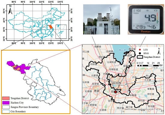
Figure 1. Geospatial location of the co-location site and the LCS (model: Temtop M10+) used for correction experiments.

2.2. Temtop M10+ LCS

In this study, the LCS used in the calibration experiment was the Temtop M10+ (upper right in Figure 1) that reported PM_2.5 concentrations with a native 1-min time resolution. This device integrates a built-in Temtop M2000 2nd-generation sensor, which measures PM_2.5 mass concentrations based on the light-scattering principle. Some previous independent evaluations by South Coast AQMD’s AQ-SPEC program show that (i) in field deployments, the sensor’s PM_2.5 shows strong correlations with FEM reference instruments (R² ≈ 0.76–0.83 using 5-min means); (ii) under laboratory conditions (20 °C, 40% RH), PM_2.5 correlations with a FEM GRIMM are very strong (R² > 0.99), but the device tends to overestimate relative to the FEM [30]. Given these characteristics, we treat the M10+/M2000 output as a stable, precise optical signal that benefits from co-location calibration to correct for systematic bias before use in our analyses. The monitoring campaign spanned six consecutive days, among which five full days provided valid paired measurements from both the LCS and the reference station. In total, 120 hourly data points were obtained for the subsequent model development.

2.3. Meteorological Variables

To account for the comprehensive effects of meteorological factors on PM_2.5 LCS measurements, this study incorporated multiple meteorological variables—including boundary layer height (BLH), 2 m temperature (T2m), 10 m u-component of wind speed (U10), surface pressure (SP), 10 m v-component of wind speed (V10), and relative humidity (RH)—in the development of the LCS correction models. Figure 2 shows the hourly time series of these meteorological variables during the study period at the co-location site.

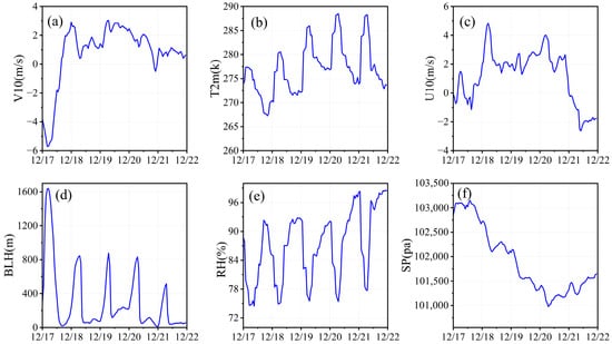
Figure 2. Hourly time series of meteorological variables during the study period: (a) V10; (b) T2m; (c) U10; (d) BLH; (e) RH; and (f) SP.

2.4. LCS Calibration Method

In this study, we applied an observation bias correction method to adjust the PM_2.5 measurements from the LCS. We assume that the PM_2.5 concentration measured by the reference fixed monitoring station (RFMS) at time t is denoted as $y_R^t$; thus, the observational time series can be expressed as $Y_R=\left\{y_R^t\left|t=1,2,\dots ,n\right.\right\}$. The PM_2.5 concentration measured by the LCS at time t is denoted as $y_L^t$; thus, the observational time series can be expressed as $Y_L=\left\{y_L^t\left|t=1,2,\dots ,n\right.\right\}$. Thus, a bias $Y_{Bias}$ exists between them as:

$$Y_{Bias}=Y_R-Y_L=\{y_B^t=y_R^t-y_L^t\left|t=1,2,\dots ,n\right.\}$$

(1)

We simply assume that this part of the observational error is caused by ambient meteorological conditions (although in reality the situation is more complex, as LCS devices themselves have instrumental observation errors, which manufacturers have already addressed through other correction methods in this study). Under this theoretical assumption, the observation bias $Y_{Bias}$ can be further expressed as a mathematical model of various meteorological variables:

$$Y_{Bias}=F(X)=F(x_1^t,x_2^t,\dots ,x_m^t)$$

(2)

where $x_m^t$ denotes the value of the m-th meteorological variable at time t, and F(X) is the mathematical model that regresses the PM_2.5 measurement bias and the most important meteorological variables. This mathematical model is constructed using four different types of ML algorithms, and the final model is selected from among them based on its optimal performance. The fundamental principles of these ML algorithms will be described in detail in the next subsection.

Once this model is established based on PM_2.5 observations from the co-location site, it can be used to correct LCS observations at other locations under different monitoring environments. Specifically, we only need to obtain the relevant meteorological parameters at the current location of an LCS site and input them into the established model to calculate the corresponding correction bias. By adding this correction bias to the original LCS PM_2.5 measurements, the corrected LCS PM_2.5 concentration data can then be obtained.

2.5. Machine Learning Algorithms

In this study, a set of machine learning algorithms with varying levels of model complexity (from simple to complex) was selected to comprehensively evaluate the calibration performance for low-cost PM_2.5 sensors. The chosen models represent a balanced combination of interpretability, computational efficiency, and predictive capability, making them suitable for both methodological comparison and practical deployment in real-world air quality monitoring applications. DTR was included as a simple and highly interpretable model that provides baseline performance with minimal computational requirements. RF and SVR were selected as medium-complexity traditional ML algorithms that are widely used and well established for nonlinear regression tasks. These models offer strong robustness and generalizability, making them representative of classical ML approaches applicable to sensor calibration. To incorporate more advanced modeling capabilities, LSTM networks were employed as a complex deep learning method capable of capturing temporal dependencies and nonlinear relationships inherent in atmospheric pollutant measurements. Furthermore, following suggestions from peer reviewers, two additional recurrent neural network architectures—GRU and BiLSTM—were included to explore whether deeper and more sophisticated neural structures could further enhance calibration accuracy.

2.5.1. Random Forest

Random forest (RF) is a non-parametric ensemble learning algorithm that performs regression by constructing multiple decision trees and aggregating their outputs [31]. By introducing randomness in both data sampling and feature selection, RF effectively reduces the high variance and overfitting problems associated with single decision trees, thereby improving the model’s generalization ability and predictive performance [32]. During model construction, the algorithm first employs bootstrap sampling to generate multiple subsets $\{D_1,D_2,\dots ,D_T\}$ from the original training dataset $D={\{(x_i,y_i)\}}_{i=1}^N$, with replacement. Each subset is then used to train a regression tree. At each node split, instead of considering all features F, a random subset F_m (m ≪ ∣F∣) is selected to determine the best splitting feature and threshold that maximizes the split gain [33,34]. This “double-randomization” mechanism—randomness in both samples and features—reduces correlations among individual trees and enhances the robustness of the overall model.

Once all trees are trained, the prediction for a new input sample x is obtained by averaging the outputs of all regression trees [34]:

$$\widehat{y}={\displaystyle \frac{1}{T}}{\displaystyle \sum _{t=1}^T{h}_t(x)}$$

(3)

where T is the total number of trees in the forest and h_t(x) denotes the prediction of the t-th regression tree for input x. This ensemble averaging significantly reduces the instability of individual trees and improves predictive accuracy. RF also provides a natural way to evaluate feature importance. By calculating the decrease in mean squared error (MSE) caused by a feature when used for splitting, its contribution to the model can be quantified.

2.5.2. Support Vector Regression

Support Vector Regression (SVR) is an extension of the Support Vector Machine (SVM) for regression tasks. It aims to construct an optimal regression function in a high-dimensional feature space to capture the relationship between input variables and continuous target variables [35]. The core idea of SVR is to fit the training data within a predefined tolerance margin while keeping the regression function as flat as possible, thereby enhancing the model’s generalization capability and robustness to noise [36].

Given a training dataset $D={\{(x_i,y_i)\}}_{i=1}^N$, where $x_i\in R^d$ is the input feature vector and $y_i\in R$ is the target variable, SVR seeks a regression function of the form [37]:

$$f(x)=w^T\varphi (x)+b$$

(4)

Here, ϕ(x) is a nonlinear mapping function that projects the input data into a high-dimensional feature space, while w and b are the weight vector and bias term, respectively. SVR minimizes the model complexity, represented by ||w||², while allowing prediction errors within an ϵ-insensitive tube. Due to its strong generalization ability, robustness to noise, and capability to model nonlinear relationships even with limited samples and high-dimensional data, SVR has been widely applied in the field of environmental modeling.

2.5.3. Long Short-Term Memory

Long Short-Term Memory (LSTM) is a special type of recurrent neural network (RNN) designed to model sequential data and capture long-range dependencies that standard RNNs often fail to learn due to vanishing or exploding gradient problems [38]. By introducing a memory cell and a gating mechanism, LSTM effectively retains relevant historical information over extended time steps, making it particularly suitable for time series prediction tasks such as air quality modeling [39].

An LSTM unit consists of three key gates—the input gate, the forget gate, and the output gate—which jointly regulate the flow of information through the network. At each time step t, given the input vector x_t and the previous hidden state h_t−1, the gating operations are defined as follows [40,41]:

Forget gate: Controls how much of the previous cell state should be retained:

$$f_t=\sigma (W_f[h_{t-1},x_t]+b_f)$$

(5)

Input gate: Determines how much new information should be added to the cell state:

$$i_t=\sigma (W_i[h_{t-1},x_t]+b_i)$$

(6)

$${\overline{C}}_t=\tanh (W_C[h_{t-1},x_t]+b_C)$$

(7)

Cell state update: Combines retained memory and new information:

$$C_t=f_t\odot C_{t-1}+i_t\odot {\overline{C}}_t$$

(8)

Output gate: Controls how much of the updated cell state contributes to the hidden state:

$$o_t=\sigma (W_o[h_{t-1},x_t]+b_o)$$

(9)

$$h_t=o_t\odot \tanh (C_t)$$

(10)

Here, σ() denotes the sigmoid activation function, tanh() is the hyperbolic tangent function, ⊙ represents element-wise multiplication, C_t is the cell state, and h_t is the hidden state at time t. The gating mechanism allows LSTM to dynamically adjust the retention, removal, and integration of information, thereby overcoming the limitations of standard RNNs in capturing long-term temporal dependencies. Because of these properties, LSTM has been widely applied in sequential modeling tasks such as time series forecasting, natural language processing, and environmental data prediction.

2.5.4. Decision Tree Regression

DTR is a non-parametric supervised learning method that predicts a continuous target variable by recursively partitioning the feature space into a set of disjoint regions and fitting a simple prediction model (typically a constant value) within each region [42]. Its core idea is to split the data into increasingly homogeneous subsets based on feature values, thereby minimizing prediction error at each node [43].

Given a training dataset $D={\{(x_i,y_i)\}}_{i=1}^N$, where $x_i\in R^d$ denotes the feature vector and $y_i\in R$ the target variable, the algorithm starts from the root node containing the entire dataset and searches for the feature j and threshold s that best split the data into two subsets [43,44]:

$$R_1(j,s)=\left\{X\right|x_j\le s\},\hspace{1em}{R}_2(j,s)=\{X|x_j>s\}$$

(11)

The optimal split is chosen to minimize the sum of squared errors (SSE) across the two child nodes [44]:

$$\underset{j,s}{\min }\left[{\displaystyle \sum _{x_i\in R_1(j,s)}{(y_i-{\overline{y}}_{R_1})}^2}+{\displaystyle \sum _{x_i\in R_2(j,s)}{(y_i-{\overline{y}}_{R_2})}^2}\right]$$

(12)

where ${\overline{y}}_{R_1}$ and ${\overline{y}}_{R_2}$ are the mean values of the target variable in regions R₁ and R₂, respectively. This splitting process is applied recursively to each resulting node until a stopping criterion is met, such as reaching a maximum tree depth or a minimum number of samples per leaf node.

For a new input x, the prediction $\widehat{y}$ is determined by the average of the target values of the training samples in the terminal region R_m to which x belongs [44]:

$$\widehat{y}={\displaystyle \frac{1}{\left|R_m\right|}}{\displaystyle \sum _{x_i\in R_m}{y}_i}$$

(13)

DTR is intuitive, interpretable, and capable of capturing nonlinear relationships without requiring feature scaling or prior assumptions about the data distribution.

2.5.5. Gated Recurrent Unit

The Gated Recurrent Unit (GRU) is an improved recurrent neural network architecture designed to more effectively model temporal dependencies in sequential data while reducing computational complexity relative to traditional LSTM networks [45]. GRU introduces a streamlined gating mechanism composed of an update gate and a reset gate. The update gate controls the extent to which past information is retained, enabling the model to capture long-range temporal dependencies without suffering from vanishing gradients. The reset gate determines how much of the previous state should be ignored when incorporating new input information, allowing the network to adaptively focus on short-term patterns when necessary. Because GRU combines memory and gating operations into a simplified structure, it requires fewer parameters than LSTM, resulting in faster training and lower computational cost while maintaining competitive performance [46]. This balance between efficiency and modeling capability makes GRU suitable for applications involving time-dependent environmental data, such as air pollution monitoring and sensor calibration.

2.5.6. Bidirectional Long Short-Term Memory

The Bidirectional Long Short-Term Memory (BiLSTM) network is an extension of the traditional LSTM architecture designed to capture temporal dependencies in both forward and backward directions [47]. Unlike standard LSTM, which processes sequences only from past to future, a BiLSTM consists of two parallel LSTM layers: one that processes the input sequence in the forward direction and another that processes it in the reverse direction. By combining the outputs of these two layers, the model gains access to both preceding and succeeding contextual information at each time step [48].

2.5.7. Algorithm Complexities

A computational complexity analysis of the above six ML algorithms based on their algorithmic properties was also provided. These models differ in training time complexity, memory cost, parameter size, and capacity to model nonlinear or temporal dependencies. Tree-based models (DTR and RF) typically have training complexities of O(n⋅d⋅log n) and O(T⋅n⋅log n), respectively, where n is the number of samples, d the feature dimension, and T the number of trees. Their memory costs are O(n) and O(T·n), respectively. SVR exhibits a higher training complexity of O(n³) due to kernel matrix inversion, making it more computationally demanding for large n. It has a prediction complexity of O(s·d) where s is the number of support vectors. Deep learning models (LSTM, GRU, BiLSTM) have complexities on the order of O(n⋅h²⋅L), where h is the number of hidden units, and L is the number of layers. The parameter size increases with the number of hidden units h and layers L. These objective complexity measures reflect the computational cost and scalability of different algorithms.

2.6. Hyperparameter Optimization

To ensure fair and reliable comparison among the machine learning and deep learning models, all algorithms were tuned through a unified hyperparameter optimization procedure. Key hyperparameters for each model were optimized using the Particle Swarm Optimization (PSO) algorithm, combined with the corresponding optimization functions in MATLAB (R2023a). Parameters not included in the optimization search space were kept at MATLAB’s default settings. This approach provides improved model stability and prevents biased performance caused by suboptimal or unbalanced parameter choices. For the RF model, the function optimize_fitrtreebag was used to optimize the number of trees and minimum leaf size, yielding optimal values of 180 trees and a leaf size of 1. For SVR, optimize_fitrsvm tuned the BoxConstraint, KernelScale, and Epsilon parameters, with final values of 2.22, 4.25, and 0.001, respectively. The DTR model was optimized using optimize_fitrtree, which identified a minimum leaf size of 4 as optimal. For deep learning models, customized optimization functions were applied. The LSTM model was tuned using optimize_fitrLSTM_att, resulting in 44 layers, 20 hidden units, and a dropout rate of 0.001. The GRU model was optimized with optimize_fitrGRU_att, producing 48 layers, 28 hidden units, and a dropout rate of 0.17. Finally, the BiLSTM model was optimized using optimize_fitrBiLSTM, which selected 86 layers and a dropout rate of 0.39 as the best-performing configuration.

2.7. Model Development and Validation

To ensure robust model training and fair performance evaluation, the complete dataset collected from the co-location experiment was randomly divided into three subsets: a training set (80%, 96 data points), a validation set (10%, 12 data points), and a testing set (10%, 12 data points). The training set was used to fit the ML models, the validation set was employed for model tuning and hyperparameter optimization, and the testing set was reserved for final performance evaluation. Given that the random data splitting process can introduce variability and uncertainty in model performance, the entire modeling and evaluation procedure was repeated ten times in a bootstrap fashion. In each repetition, the dataset was randomly resampled and re-split following the 8:1:1 ratio. The final performance metrics were reported as the mean across the ten bootstrap iterations.

Model performance was quantitatively assessed using four commonly adopted statistical indicators: mean absolute error (MAE), mean absolute percentage error (MAPE), root mean square error (RMSE), and the coefficient of determination (R²). MAE and RMSE measure the absolute and squared deviations between predictions and observations, respectively, indicating model accuracy in units consistent with the target variable. MAPE provides a dimensionless measure of relative error, facilitating comparison across different concentration ranges. R² evaluates the proportion of variance in the reference observations that is explained by the model predictions, reflecting the overall goodness of fit. These metrics allowed a comprehensive evaluation of the predictive accuracy, bias, and reliability of each calibration model on the training, validation, and testing datasets.

The best-performing model for each algorithm was determined based on its average performance on the validation datasets across the ten bootstrap iterations. Specifically, the model configuration yielding the lowest mean RMSE and MAE, together with the highest mean R², was selected as the optimal model. This model was subsequently applied to the independent testing dataset to assess its final predictive performance and generalization capability. All data preprocessing, machine learning model development, performance evaluation, and figure generation were conducted using MATLAB.

3. Results

3.1. Colocation PM_2.5 Observations

Figure 3 presents the time series of co-located PM_2.5 observations obtained from the reference fixed monitoring station (RFMS) and the low-cost sensor (LCS) during the experiment period. The red and blue lines represent PM_2.5 concentrations measured by the RFMS and LCS, respectively, while the green line shows their difference (RFMS–LCS). Overall, both instruments exhibited highly consistent temporal variation patterns, with the LCS successfully capturing the major pollution peaks and clean-air episodes observed by the RFMS. The two datasets showed a strong linear correlation (R² = 0.90, see Figure 4), indicating excellent temporal agreement. However, the LCS tended to slightly underestimate PM_2.5 concentrations relative to the RFMS, particularly during high-pollution episodes, with a mean bias of –7.49 µg/m³ and a root mean square error (RMSE) of 10.17 µg/m³. The difference between the two measurements (RFMS–LCS) fluctuated within a narrow range, further confirming the stability and reliability of the LCS under varying pollution levels. These results demonstrate that the Temtop M10+ LCS can effectively monitor the temporal variations of PM_2.5 concentrations, although appropriate calibration may be required to correct systematic underestimation during pollution episodes.

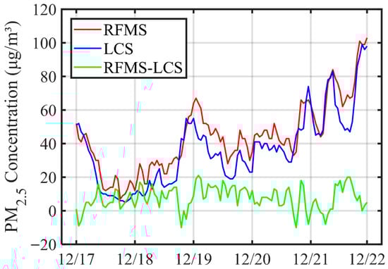
Figure 3. Time series comparison of co-located PM_2.5 observations from the reference fixed monitoring station (RFMS) and the low-cost sensor (LCS).

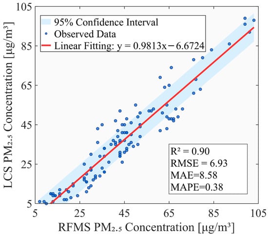
Figure 4. Scatter plot comparing the RFMS and LCS observations of PM_2.5 concentrations.

Figure 4 illustrates the scatter plot comparing the PM_2.5 concentrations measured by the RFMS and LCS. A strong linear correlation was observed between the two datasets (R² = 0.90), indicating that the LCS measurements closely followed the variations recorded by the reference instrument. The fitted regression line (y = 0.9813x − 6.6724) shows a slope close to unity, suggesting that the LCS can effectively capture the magnitude and trend of PM_2.5 concentrations with only a minor systematic underestimation. The relatively narrow 95% confidence interval (shaded region) further confirms the consistency between the two measurements across the observed concentration range. In terms of quantitative performance, the RMSE and MAE were 6.93 µg/m³ and 8.58 µg/m³, respectively, reflecting good overall agreement between the LCS and the RFMS measurements. The MAPE was 0.38 (equivalent to 38%), indicating that, on average, the LCS deviated from the reference measurements by approximately 38%. This level of accuracy is within the acceptable range for low-cost PM_2.5 sensors and demonstrates that the LCS provides a reliable estimation of ambient PM_2.5 concentrations under most conditions even without calibration.

Figure 5 shows the boxplots of PM_2.5 concentrations measured by the RFMS and LCS, along with the distribution of their differences (RFMS–LCS). The boxes represent the interquartile range (25th–75th percentile), the horizontal red line denotes the median, the small square indicates the mean, and whiskers extend to 1.5 times the interquartile range (IQR). Red diamonds represent outliers. Overall, RFMS and LCS datasets exhibit similar distribution patterns, suggesting that the LCS effectively captures the temporal variations in PM_2.5 levels. However, the LCS tends to slightly underestimate PM_2.5 concentrations relative to the RFMS, as indicated by the lower median and mean values. The difference distribution (RFMS–LCS) further illustrates this bias, with most values clustered near zero and a small positive median and mean, implying a systematic underestimation by the LCS. The narrow interquartile range of the difference plot indicates good consistency between the two measurements for the majority of data points, while a few high outliers reflect occasional deviations at higher concentration levels.

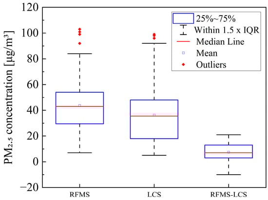
Figure 5. Boxplots of PM_2.5 concentrations measured by the RFMS and LCS, along with the distribution of their differences (RFMS–LCS).

These results demonstrate that, even without calibration, the LCS provides concentration estimates that are generally consistent with reference-grade measurements, though with a minor bias that can be effectively corrected through subsequent calibration procedures.

3.2. Calibration Modelling Results

Six ML algorithms—RF, SVR, LSTM, DTR, GRU, and BiLSTM—were applied to regress the measurement biases against the meteorological variables. The performance of calibration models was assessed on the training, validation, and testing datasets following the procedures described in Section 2.6.

The fitting performance of the six ML models, as illustrated in Figure 6, reveals clear differences in their ability to reproduce the observed PM_2.5 differences between the LCS and the reference station. The solid black line represents the 1:1 reference line, and the color scale indicates the data density, where red denotes regions with higher point density (H) and blue denotes lower density (L). All models show a strong linear relationship between observed and predicted values, with varying degrees of dispersion depending on model complexity. Among them, RF demonstrates the strongest fitting accuracy, with a regression slope closest to unity and an R² of 0.99, indicating excellent agreement between predicted and observed values across the full concentration range. Data points lie tightly around the 1:1 line, reflecting strong robustness and minimal bias. DTR also performs exceptionally well, achieving an R² of 0.98, with a near-unity slope that indicates consistent predictive capability. The scatter distribution is compact and symmetrical, suggesting that DTR effectively captures nonlinear relationships without exhibiting severe overfitting, despite its relatively simple model structure. In contrast, SVR exhibits noticeable underperformance, only with a fitting R² of 0.72. The scatter points deviate more widely from the 1:1 line, especially at medium-higher concentration levels, leading to a visible increase in prediction bias. This result suggests that SVR is less capable of capturing complex nonlinear patterns using the available short-term dataset. For the deep learning methods, GRU and BiLSTM both deliver strong performance, with R² values of 0.91 and 0.92, respectively. Their scatter patterns show better linearity and reduced bias compared to SVR, especially in medium concentration ranges. Among the deep learning architectures, BiLSTM demonstrates slightly better fitting, benefitting from bidirectional temporal dependency learning. LSTM, however, produces the weakest fitting among the deep learning models, with an R² of 0.83. The scatter points show greater dispersion, particularly in high and low concentration regions, indicating that LSTM may require larger datasets to fully leverage its temporal modeling capability. Overall, the fitting results confirm that RF and DTR provide the most accurate and stable performance, followed by GRU and BiLSTM as competitive deep learning approaches. SVR and LSTM show clear limitations within the context of this short-term dataset. These findings highlight the importance of model complexity and data availability in determining calibration performance for low-cost PM_2.5 sensors.

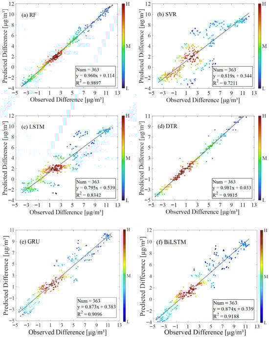
Figure 6. Scatter plots comparing the observed and predicted PM_2.5 concentration differences for the training dataset using six ML algorithms: (a) RF, (b) SVR, (c) LSTM, (d) DTR, (e) GRU, and (f) BiLSTM.

Table 1 presents a statistical summary of the model performance across the training, validation, and testing datasets. A comprehensive comparison of the calibration results across the six ML algorithms shows clear differences in model performance and generalization ability. Among all models, RF consistently demonstrates the best overall accuracy, with R² values of 0.99 (training), 0.94 (validation), and 0.94 (testing). The stability of these scores across all phases indicates strong generalization and robustness, which is further supported by their low RMSE, MAE, and MAPE values. DTR also performs well, achieving R² values of 0.98, 0.95, and 0.92 for training, validation, and testing, respectively. Although slightly less accurate than RF, DTR demonstrates strong interpretability and reliable predictive performance. Its lower complexity contributes to reduced risk of overfitting, making it a practical option for real-world sensor calibration when computational resources are limited. In contrast, SVR shows the weakest performance among the traditional ML models. The validation and testing R² values drop to 0.58 and 0.77, respectively, and the error metrics (particularly MAPE = 4.77 in testing) indicate difficulty in fitting the nonlinear sensor–atmosphere relationship. This suggests that SVR is less suited for this dataset and may require larger training samples or more careful parameter tuning to achieve competitive accuracy. For the deep learning models, LSTM, GRU, and BiLSTM all achieve moderate to good performance, with testing R² ranging between 0.86–0.98. BiLSTM performs the best among the deep learning methods, with R² values of 0.92 (training), 0.89 (validation), and 0.98 (testing), reflecting its ability to leverage bidirectional temporal dependencies. GRU exhibits competitive performance as well, outperforming LSTM on testing data. However, the larger gap between training and testing metrics for LSTM (0.83 → 0.86) and for GRU (0.91 → 0.96) suggests higher sensitivity to data scarcity and potential overfitting under small-sample conditions.

Table 1. Statistical summary of the calibration modelling performance of six ML algorithms.

Model	Metrics	Training	Validation	Testing
RF	R2	0.99	0.94	0.94
	RMSE	0.42	1.01	1.07
	MAE	0.30	0.76	0.79
	MAPE	0.27	0.62	0.72
SVR	R2	0.71	0.58	0.77
	RMSE	2.15	2.03	2.87
	MAE	1.67	1.59	2.16
	MAPE	1.48	1.59	4.77
LSTM	R2	0.83	0.76	0.86
	RMSE	1.62	1.60	2.18
	MAE	1.34	1.36	1.61
	MAPE	1.23	1.15	2.80
DTR	R2	0.98	0.95	0.92
	RMSE	0.52	1.13	0.86
	MAE	0.32	0.65	0.67
	MAPE	0.76	0.41	0.26
GRU	R2	0.91	0.90	0.96
	RMSE	1.25	1.30	0.80
	MAE	1.00	1.13	0.70
	MAPE	0.76	1.28	0.40
BiLSTM	R2	0.92	0.89	0.98
	RMSE	1.19	1.33	0.33
	MAE	0.94	1.11	0.52
	MAPE	0.71	1.34	0.31

Overall, the results indicate that RF provides the most balanced and reliable performance, followed by DTR as a strong lightweight alternative. Deep learning models demonstrate promising predictive capability, particularly BiLSTM and GRU, but their performance depends more heavily on dataset size and temporal richness. SVR shows clear limitations in this context. These findings suggest that, under small-sample scenarios such as short-term co-location experiments, ensemble methods like RF remain the most robust choice for LCS calibration. Consequently, RF was selected as the optimal model in this study and subsequent discussion.

3.3. Model Complexity Analysis

To provide an objective comparison of the computational properties of the six ML algorithms, we evaluated their theoretical training and inference complexity, parameter size, and expected computational burden. RF and DTR exhibit training complexity on the order of O(n·d·h) per tree, with RF scaling to O(T·n·d·h) for T trees. Both offer fast inference (O(h) for DTR and O(T·h) for RF), making them computationally efficient for deployment. SVR shows the highest theoretical training cost, O(n³) with O(n²) memory due to kernel-based quadratic programming, and an inference cost proportional to the number of support vectors. For the neural models, the two-layer LSTM architecture used in this study contains approximately 53.4k trainable parameters and requires O(T(h² + h·d)) operations per layer, resulting in the largest computational burden among the deep learning models. GRU, with ~31.3k parameters, reduces computation by simplifying the gating structure, offering lower complexity for the same sequence length. The BiLSTM model processes sequences bidirectionally, doubling per-step complexity, but its parameter size (~17.2k) remains smaller than that of the stacked LSTM, positioning it between LSTM and GRU in computational cost. Overall, SVR has the highest theoretical training complexity, deep learning models require substantial sequential computation, and RF offers the best balance between computational efficiency and predictive performance in this study.

4. Discussion

In this study, we developed a comprehensive ML-based calibration framework for low-cost PM_2.5 sensors that integrates diverse meteorological predictors to improve measurement accuracy. Using continuous co-location experiments conducted in Tongshan District of Xuzhou City, the hourly PM_2.5 data obtained from a Temtop M10+ series LCS were compared against those from a co-location reference monitoring station. The biases between the two datasets were modeled as functions of key meteorological variables through multiple ML algorithms, including RF, SVR, LSTM, DTR, GRU, and BiLSTM. The optimal model was selected based on its superior predictive performance across training, validation, and testing datasets. For other models of LCS used in another city, we can also establish ML calibration models following this framework, and then add the corrected biases to the original measurements for data calibration.

Our study demonstrates that the latest LCS can provide a relatively reliable monitoring of ambient PM_2.5 concentrations under most conditions, even without calibration. Compared with previous studies, the results of this work indicate that the baseline performance of LCSs has substantially improved in recent years. For example, Park et al. [28] reported that the raw PM_2.5 data from their LCS (Sensirion SPS 30) exhibited only a moderate correlation with reference-grade instruments (R² = 0.59). In contrast, our study found that even without calibration, the LCS measurements showed a strong linear relationship with the reference data (R² = 0.90). This improvement suggests that recent generations of LCSs have benefited from advancements in optical particle detection, onboard signal processing, and factory calibration, resulting in more reliable measurements across a broader range of concentrations. Although differences in sensor models, environmental conditions, and aerosol characteristics may also contribute to the performance gap between studies, the overall trend clearly reflects a technological evolution toward higher intrinsic accuracy of LCS devices. Nevertheless, our findings also demonstrate that applying ML calibration incorporating meteorological predictors can further minimize systematic bias and enhance model generalization, indicating that the combination of improved sensor hardware and data-driven calibration methods holds great promise for large-scale, high-resolution air quality monitoring.

Our study also demonstrates that incorporating a wider range of meteorological predictors significantly enhances the accuracy and robustness of LCS calibration compared with conventional approaches that typically consider only relative humidity (RH) and temperature. Building on prior work, we compiled the reported accuracies of different ML-based calibration schemes and contrasted them with our results. Park et al. [28] evaluated raw LCS readings (R² = 0.59) and three calibration models—MLR (R² = 0.80), DNN (R² = 0.90), and a HybridLSTM (R² = 0.93)—and showed the HybridLSTM reduced RMSE by 41–60% versus raw data and by 30–51% versus MLR on the same test sets, using humidity and temperature as meteorological inputs alongside sensor PM_2.5. Kumar et al. [49] assessed several algorithms seasonally with a PurpleAir LCS and reported that RF performed best when limited to a small set of meteorological covariates (typically RH, temperature, and wind speed), attaining R² improvements from ~0.66–0.73 pre-calibration to ~0.94–0.96 post-calibration and test-set RMSE on the order of ~0.7–1.2 µg/m³ depending on season. In comparison, our framework—trained with a broader feature set that expands beyond RH, temperature, and wind speed to include six meteorological predictors—achieved the highest overall accuracy with RF (R² ≈ 0.99/0.94/0.94 for training/validation/testing, with consistently lower RMSE and MAE across bootstrap splits). By integrating six meteorological variables in our modeling framework, this study provides a more comprehensive description of the meteorological influences on LCS performance, allowing a more precise correction of PM_2.5 sensor readings under diverse atmospheric conditions. Additional meteorological variables help capture complex processes such as hygroscopic growth, dispersion dynamics, and boundary-layer stability, which jointly modulate the optical response of PM_2.5 sensors. Consequently, our results highlight the advantage of a multi-factor ML calibration framework that leverages richer meteorological information to achieve more reliable and transferable LCS corrections.

Our results suggest that tree-based/ensemble models (especially RF) outperform kernel-based and sequential models in this LCS calibration context. The consistently strong performance of the RF algorithm observed in this study aligns with previous research findings, confirming its suitability for calibrating low-cost PM_2.5 sensors. Wang et al. [32] reported that their RF-based calibration of a Hike HK-B3 monitor achieved an R² of 0.98, substantially outperforming the traditional linear regression model (R² = 0.87) under various temperature and humidity conditions. Similarly, our RF model yielded an R² of 0.99 (training) and 0.94 (validation and testing), accompanied by the lowest RMSE, MAE, and MAPE values among all tested ML approaches, further verifying the robustness of RF in capturing complex nonlinear relationships between sensor deviations and meteorological covariates. The RF algorithm’s superior performance can be attributed to its ensemble learning nature, which integrates multiple decision trees to minimize overfitting and effectively handle nonlinear and multicollinear interactions among predictor variables. Unlike regression-based or kernel methods that assume specific data distributions, RF can flexibly model intricate dependencies between PM_2.5 measurement biases and meteorological factors such as humidity, temperature, wind, and pressure. This adaptability enables it to generalize well across varying pollution levels and meteorological conditions. Additionally, the variable importance metrics generated by RF provide valuable interpretability, revealing how different meteorological factors contribute to sensor measurement biases—a feature especially useful for optimizing sensor deployment and calibration strategies. Taken together, both the present study and previous literature demonstrate that RF offers a balanced combination of accuracy, robustness, and interpretability, making it one of the most reliable algorithms for PM_2.5 LCS calibration. Its capability to model complex meteorological influences supports its broader application in large-scale, high-resolution air quality monitoring networks.

Our results indicate that computational complexity and model capacity significantly influence calibration performance, especially under small-sample conditions. Although deep learning models such as LSTM, GRU, and BiLSTM have the capacity to capture nonlinear temporal dependencies, their performance is more sensitive to data availability, and overfitting may occur under limited sample conditions. Medium-complexity models (RF and SVR) provide a balance between computational efficiency and predictive power, with RF showing superior performance and stability. The simple DTR model also achieved strong accuracy with minimal computational requirements, demonstrating that low-complexity models may be sufficient when the data size is small. This analysis highlights the importance of selecting model complexity appropriate to the data scale and practical deployment conditions for LCS calibration.

Overall, this study demonstrates that low-cost PM_2.5 sensors, after appropriate ML-based calibration, can achieve accuracy comparable to that of reference-grade instruments, supporting their use as a cost-effective and scalable monitoring solution. The proposed calibration framework effectively corrects measurement biases by integrating multiple meteorological predictors, thereby enhancing the reliability of PM_2.5 LCS measurements under diverse meteorological conditions. This advancement highlights the potential of LCS networks to supplement regulatory monitoring systems, enabling dense spatial coverage and high-resolution exposure assessment at a fraction of the cost of conventional networks.

Although the present framework was only tested using co-location PM_2.5 data from Xuzhou, its structure is inherently scalable and transferable. Because the method relies on generalizable statistical relationships between LCS deviations, reference measurements, and meteorological parameters, it can be readily adapted to other geographic regions and sensor models with minimal retraining effort. Moreover, in addition to PM_2.5 calibrations, the ML–based correction framework developed in this study demonstrates strong potential for broader applicability to other air pollutants measured by low-cost sensors. Although this work focuses specifically on PM_2.5, the structure of the proposed model and the multivariable integration strategy allow for adaptation to pollutants with similar physicochemical characteristics and measurement mechanisms. For example, PM₁₀ shares comparable sources, atmospheric behaviors, and light-scattering measurement principles with PM_2.5; therefore, the selected meteorological predictors are likely to remain relevant and effective when extending the model to PM₁₀ calibration. For gaseous pollutants such as O₃, VOCs, NO, NO₂, CO, and SO₂, the applicability of the framework also remains feasible but requires additional consideration. Unlike PM_2.5 sensors, which typically rely on optical scattering techniques, most low-cost gas sensors use electrochemical or metal-oxide semiconductor technologies that exhibit different sensitivities to environmental conditions. Consequently, the optimal set of input variables may differ, as these sensors are often more strongly influenced by multiple environmental and meteorological factors, as well as cross-sensitivity to interfering gases. These factors may lead to greater variability in calibration performance when compared with particulate measurements. Nevertheless, by incorporating pollutant-specific environmental predictors and sensor behavior characteristics, the general modeling approach presented here can be adapted to support the calibration of a broad range of low-cost air quality sensors. Overall, the framework proposed in this study provides a transferable foundation for correcting multiple types of sensor measurements. Future work will include extending the model to additional pollutants and evaluating its performance across varying sensor technologies and environmental conditions to further validate its generalizability.

This study also holds broader implications for environmental sciences. Reliable and spatially resolved air pollution data are fundamental for understanding the dynamics of air pollution, aerosol–climate interactions, and human exposure to changing environmental conditions. By integrating various meteorological predictors into an ML–based calibration framework, this study provides a pathway to enhance the accuracy and representativeness of LCS PM_2.5 observations. Such improvement in observation quality not only supports the assessment of air quality and environmental health but may also contribute valuable input data for studying regional and global environmental changes. Therefore, beyond methodological advancement, our work also strengthens the data foundation and analytical capacity necessary for developing environmental science and management.

A limitation of this study lies in the relatively limited size of the experimental dataset. It is important to emphasize that the dataset used in this study—although sufficiently representative for demonstrating the applicability of the proposed method—remains inherently limited in size. The constrained data volume may still introduce uncertainty into the evaluation process. Therefore, the generalizability of the model beyond the current experimental setting may not be fully verified at this stage. Future work will prioritize the integration of larger multi-site datasets or publicly accessible sensor–meteorology datasets to further assess cross-site robustness and improve model reliability. We acknowledge this limitation explicitly and encourage subsequent studies to validate and extend our framework under broader real-world conditions. To mitigate this issue, we adopted a rigorous validation strategy in which the entire modeling and assessment procedure was repeated ten times in a bootstrap manner, thereby reducing the variability caused by random data splitting. Nevertheless, the restricted dataset remains an inherent constraint that may limit the generalizability of the findings. Future work will benefit from incorporating additional publicly available datasets to further validate and strengthen the robustness of the proposed approach. It is also important to acknowledge that, in long-term air quality studies, the evolution of meteorological conditions across seasons can significantly influence PM_2.5 concentrations. Variables such as precipitation, fog, solar radiation, and ultraviolet radiation are known to affect particle formation, dispersion, and removal processes. However, the dataset used in this study spans only six days, during which seasonal variability does not meaningfully manifest. As a result, the absence of seasonal indicators has limited impact on the calibration outcomes for this short-term co-location experiment. In addition, although a broader set of meteorological parameters could theoretically enhance calibration performance, the incorporation of too many input variables under a small-sample setting is likely to introduce overfitting and reduce model reliability. For this reason, we selected six meteorological variables that are most directly relevant to PM_2.5 behavior and LCS performance. This selection strikes a balance between representing key atmospheric influences and maintaining the robustness of model training under limited data availability. Future research will extend this work using longer-term and larger datasets, which will allow the integration of additional meteorological factors and explicit consideration of seasonal cycles. Such efforts are expected to improve model generalizability and provide deeper insight into the dynamic interactions between pollutant levels, sensor behavior, and evolving meteorological conditions.

5. Conclusions

In this study, we developed an ML-based calibration framework for low-cost PM_2.5 sensors that integrates multiple meteorological predictors to improve measurement accuracy and robustness. Continuous co-location measurements were conducted in Tongshan District, Xuzhou City, using a Temtop M10+ series LCS and an RFMS. The biases between the LCS and RFMS measurements were modeled using six ML algorithms—RF, SVR, LSTM, DTR, GRU, and BiLSTM. The comparative modeling results demonstrated substantial differences in predictive performance among these algorithms. RF achieved the best overall accuracy with R² values of 0.99 (training), 0.94 (validation), and 0.94 (testing), and correspondingly low RMSE (0.42–1.07 µg/m³), MAE (0.30–0.79 µg/m³), and MAPE (0.27–0.72). DTR also performed well (R² = 0.98–0.95, RMSE = 0.52–1.13 µg/m³, MAE = 0.32–0.65 µg/m³, MAPE = 0.26–0.76), while LSTM and SVR exhibited comparatively lower accuracy and larger errors (LSTM: R² = 0.83–0.76, SVR: R² = 0.71–0.58). In addition, the two more advanced deep learning models, GRU and BiLSTM, achieved competitive performance, with testing R² values of 0.96 and 0.98, respectively, indicating that deep learning architectures can further enhance calibration accuracy when temporal dependencies are effectively captured. These results indicate that ensemble and tree-based models are particularly suitable for capturing the nonlinear and multivariate relationships between PM_2.5 deviations and meteorological factors.

Furthermore, even without calibration, the Temtop M10+ measurements showed a strong linear relationship with the reference data (R² = 0.90), though with a slight systematic underestimation. The proposed ML-based framework effectively reduced this bias and enhanced data reliability by integrating multiple meteorological factors.

Overall, this study demonstrates that the ML-based calibration approach—especially the RF model—offers a robust, interpretable, and scalable solution for improving the accuracy of low-cost PM_2.5 sensors. The framework provides a feasible pathway for large-scale sensor network deployment, enabling spatially dense and cost-effective air quality monitoring to complement regulatory stations and support refined air pollution exposure assessment. This study could advance the development of innovative techniques that enhance air quality assessment and support environmental research.

References

- Sokhi, R.S.; Moussiopoulos, N.; Baklanov, A.; Bartzis, J.; Coll, I.; Finardi, S.; Friedrich, R.; Geels, C.; Grönholm, T.; Halenka, T.; et al. Advances in air quality research–current and emerging challenges. Atmos. Chem. Phys. Discuss. 2021, 2021, 1–133. [Google Scholar] [CrossRef]
- Ma, X.; Morawska, L.; Zou, B.; Gao, J.; Deng, J.; Wang, X.; Wu, H.; Xu, X.; Wang, Y.; Tan, Z.; et al. Towards compliance with the 2021 WHO air quality guidelines: A comparative analysis of PM2.5 trends in Australia and China. Environ. Int. 2025, 198, 109378. [Google Scholar] [CrossRef] [PubMed]
- Fuller, R.; Landrigan, P.J.; Balakrishnan, K.; Bathan, G.; Bose-O’Reilly, S.; Brauer, M.; Caravanos, J.; Chiles, T.; Cohen, A.; Corra, L.; et al. Pollution and health: A progress update. Lancet Planet. Health 2022, 6, e535–e547. [Google Scholar] [CrossRef] [PubMed]
- Ndiaye, A.; Vienneau, D.; Flückiger, B.; Probst-Hensch, N.; Jeong, A.; Imboden, M.; Schmitz, O.; Lu, M.; Vermeulen, R.; Kyriakou, K.; et al. Associations between long-term air pollution exposure and mortality and cardiovascular morbidity: A comparison of mobility-integrated and residential-only exposure assessment. Environ. Int. 2025, 198, 109387. [Google Scholar] [CrossRef]
- Su, J.G.; Vuong, V.; Shahriary, E.; Aslebagh, S.; Yakutis, E.; Sage, E.; Haile, R.; Balmes, J.; Barrett, M. Health effects of air pollution on respiratory symptoms: A longitudinal study using digital health sensors. Environ. Int. 2024, 189, 108810. [Google Scholar] [CrossRef]
- Gu, Y.; Henze, D.K.; Liao, H. Sources of PM2.5 exposure and health benefits of clean air actions in Shanghai. Environ. Int. 2025, 195, 109259. [Google Scholar] [CrossRef]
- Jain, S.; Presto, A.A.; Zimmerman, N. Spatial modeling of daily PM2.5, NO2, and CO concentrations measured by a low-cost sensor network: Comparison of linear, machine learning, and hybrid land use models. Environ. Sci. Technol. 2021, 55, 8631–8641. [Google Scholar] [CrossRef]
- Snyder, E.G.; Watkins, T.H.; Solomon, P.A.; Thoma, E.D.; Williams, R.W.; Hagler, G.S.; Shelow, D.; Hindin, D.A.; Kilaru, V.J.; Preuss, P.W. The changing paradigm of air pollution monitoring. Environ. Sci. Technol. 2013, 47, 11369–11377. [Google Scholar] [CrossRef]
- Ma, X.; Zou, B.; Deng, J.; Gao, J.; Longley, I.; Xiao, S.; Guo, B.; Wu, Y.; Xu, T.; Xu, X.; et al. A comprehensive review of the development of land use regression approaches for modeling spatiotemporal variations of ambient air pollution: A perspective from 2011 to 2023. Environ. Int. 2024, 183, 108430. [Google Scholar] [CrossRef]
- Karagulian, F.; Barbiere, M.; Kotsev, A.; Spinelle, L.; Gerboles, M.; Lagler, F.; Redon, N.; Crunaire, S.; Borowiak, A. Review of the performance of low-cost sensors for air quality monitoring. Atmosphere 2019, 10, 506. [Google Scholar] [CrossRef]
- Kumar, P.; Morawska, L.; Martani, C.; Biskos, G.; Neophytou, M.; Di Sabatino, S.; Bell, M.; Norford, L.; Britter, R. The rise of low-cost sensing for managing air pollution in cities. Environ. Int. 2015, 75, 199–205. [Google Scholar] [CrossRef] [PubMed]
- Morawska, L.; Thai, P.K.; Liu, X.; Asumadu-Sakyi, A.; Ayoko, G.; Bartonova, A.; Bedini, A.; Chai, F.; Christensen, B.; Dunbabin, M.; et al. Applications of low-cost sensing technologies for air quality monitoring and exposure assessment: How far have they gone? Environ. Int. 2018, 116, 286–299. [Google Scholar] [CrossRef] [PubMed]
- Schneider, P.; Castell, N.; Vogt, M.; Dauge, F.R.; Lahoz, W.A.; Bartonova, A. Mapping urban air quality in near real-time using observations from low-cost sensors and model information. Environ. Int. 2017, 106, 234–247. [Google Scholar] [CrossRef] [PubMed]
- Liang, L. Calibrating low-cost sensors for ambient air monitoring: Techniques, trends, and challenges. Environ. Res. 2021, 197, 111163. [Google Scholar] [CrossRef]
- Mao, F.; Khamis, K.; Krause, S.; Clark, J.; Hannah, D.M. Low-cost environmental sensor networks: Recent advances and future directions. Front. Earth Sci. 2019, 7, 221. [Google Scholar] [CrossRef]
- De Vito, S.; Esposito, E.; Castell, N.; Schneider, P.; Bartonova, A. On the robustness of field calibration for smart air quality monitors. Sens. Actuators B Chem. 2020, 310, 127869. [Google Scholar] [CrossRef]
- Crilley, L.R.; Singh, A.; Kramer, L.J.; Shaw, M.D.; Alam, M.S.; Apte, J.S.; Bloss, W.J.; Hildebrandt Ruiz, L.; Fu, P.; Fu, W.; et al. Effect of aerosol composition on the performance of low-cost optical particle counter correction factors. Atmos. Meas. Tech. 2020, 13, 1181–1193. [Google Scholar] [CrossRef]
- Malm, W.C.; Day, D.E.; Kreidenweis, S.M.; Collett, J.L.; Lee, T. Humidity-dependent optical properties of fine particles during the big bend regional aerosol and visibility observational study. J. Geophys. Res. Atmos. 2003, 108. [Google Scholar] [CrossRef]
- Badura, M.; Batog, P.; Drzeniecka-Osiadacz, A.; Modzel, P. Regression methods in the calibration of low-cost sensors for ambient particulate matter measurements. SN Appl. Sci. 2019, 1, 622. [Google Scholar] [CrossRef]
- Okafor, N.U.; Alghorani, Y.; Delaney, D.T. Improving data quality of low-cost IoT sensors in environmental monitoring networks using data fusion and machine learning approach. ICT Express 2020, 6, 220–228. [Google Scholar] [CrossRef]
- Gao, M.; Cao, J.; Seto, E. A distributed network of low-cost continuous reading sensors to measure spatiotemporal variations of PM2.5 in Xi’an, China. Environ. Pollut. 2015, 199, 56–65. [Google Scholar] [CrossRef] [PubMed]
- Malings, C.; Tanzer, R.; Hauryliuk, A.; Kumar, S.P.; Zimmerman, N.; Kara, L.B.; Presto, A.A.; Subramanian, R. Development of a general calibration model and longterm performance evaluation of low-cost sensors for air pollutant gas monitoring. Atmos. Meas. Tech. 2019, 12, 903–920. [Google Scholar] [CrossRef]
- Zusman, M.; Schumacher, C.S.; Gassett, A.J.; Spalt, E.W.; Austin, E.; Larson, T.V.; Carvlin, G.; Seto, E.; Kaufman, J.D.; Sheppard, L. Calibration of low-cost particulate matter sensors: Model development for a multi-city epidemiological study. Environ. Int. 2020, 134, 105329. [Google Scholar] [CrossRef] [PubMed]
- Reynolds, R.; Liang, L.; Li, X.; Dennis, J. Monitoring annual urban changes in a rapidly growing portion of Northwest Arkansas with a 20-Year landsat record. Remote Sens. 2017, 9, 71. [Google Scholar] [CrossRef]
- Qin, X.; Hou, L.; Gao, J.; Si, S. The evaluation and optimization of calibration methods for low-cost particulate matter sensors: Inter-comparison between fixed and mobile methods. Sci. Total Environ. 2020, 715, 136791. [Google Scholar] [CrossRef]
- Liu, H.Y.; Schneider, P.; Haugen, R.; Vogt, M. Performance assessment of a lowcost PM2.5 sensor for a near four-month period in Oslo, Norway. Atmosphere 2019, 10, 41. [Google Scholar] [CrossRef]
- Si, M.; Xiong, Y.; Du, S.; Du, K. Evaluation and Calibration of a Low-cost Particle Sensor in Ambient Conditions Using Machine Learning Technologies. Atmos. Meas. Tech. 2019, 13, 1693–1707. [Google Scholar] [CrossRef]
- Park, D.; Yoo, G.W.; Park, S.H.; Lee, J.H. Assessment and calibration of a low-cost PM2.5 sensor using machine learning (hybridlSTM neural network): Feasibility study to build an air quality monitoring system. Atmosphere 2021, 12, 1306. [Google Scholar] [CrossRef]
- Hagan, D.H.; Isaacman-VanWertz, G.; Franklin, J.P.; Wallace, L.M.; Kocar, B.D.; Heald, C.L.; Kroll, J.H. Calibration and assessment of electrochemical air quality sensors by co-location with regulatory-grade instruments. Atmos. Meas. Tech. 2018, 11, 315–328. [Google Scholar] [CrossRef]
- Temtop. Elitech-Temtop-m2000-2nd-Generation Summary Report. 2021. Available online: http://www.aqmd.gov/aq-spec/evaluations/field (accessed on 1 September 2025).
- Zimmerman, N.; Presto, A.A.; Kumar, S.P.; Gu, J.; Hauryliuk, A.; Robinson, E.S.; Robinson, A.L. A machine learning calibration model using random forests to improve sensor performance for lower-cost air quality monitoring. Atmos. Meas. Tech. 2018, 11, 291–313. [Google Scholar] [CrossRef]
- Wang, Y.; Du, Y.; Wang, J.; Li, T. Calibration of a low-cost PM2.5 monitor using a random forest model. Environ. Int. 2019, 133, 105161. [Google Scholar] [CrossRef] [PubMed]
- Kureshi, R.R.; Mishra, B.K.; Thakker, D.; John, R.; Walker, A.; Simpson, S.; Thakkar, N.; Wante, A.K. Data-driven techniques for low-cost sensor selection and calibration for the use case of air quality monitoring. Sensors 2022, 22, 1093. [Google Scholar] [CrossRef] [PubMed]
- Breiman, L. Random forests. Mach. Learn. 2001, 45, 5–32. [Google Scholar] [CrossRef]
- Suriano, D.; Penza, M. Assessment of the performance of a low-cost air quality monitor in an indoor environment through different calibration models. Atmosphere 2022, 13, 567. [Google Scholar] [CrossRef]
- Adong, P.; Bainomugisha, E.; Okure, D.; Sserunjogi, R. Applying machine learning for large scale field calibration of low-cost PM2.5 and PM10 air pollution sensors. Appl. AI Lett. 2022, 3, e76. [Google Scholar] [CrossRef]
- Smola, A.J.; Schölkopf, B. A tutorial on support vector regression. Stat. Comput. 2004, 14, 199–222. [Google Scholar] [CrossRef]
- Jeon, H.; Ryu, J.; Kim, K.M.; An, J. The development of a low-cost particulate matter 2.5 sensor calibration model in daycare centers using long short-term memory algorithms. Atmosphere 2023, 14, 1228. [Google Scholar] [CrossRef]
- Apostolopoulos, I.D.; Fouskas, G.; Pandis, S.N. Field calibration of a low-cost air quality monitoring device in an urban background site using machine learning models. Atmosphere 2023, 14, 368. [Google Scholar] [CrossRef]
- Liu, N.; Liu, X.; Jayaratne, R.; Morawska, L. A study on extending the use of air quality monitor data via deep learning techniques. J. Clean. Prod. 2020, 274, 122956. [Google Scholar] [CrossRef]
- Hochreiter, S.; Schmidhuber, J. Long short-term memory. Neural Comput. 1997, 9, 1735–1780. [Google Scholar] [CrossRef]
- Czajkowski, M.; Kretowski, M. The role of decision tree representation in regression problems–An evolutionary perspective. Appl. Soft Comput. 2016, 48, 458–475. [Google Scholar] [CrossRef]
- Suthaharan, S. Decision tree learning. In Machine Learning Models and Algorithms for Big Data Classification: Thinking with Examples for Effective Learning; Springer: Boston, MA, USA, 2016; pp. 237–269. [Google Scholar]
- De Ville, B. Decision trees. Wiley Interdiscip. Rev. Comput. Stat. 2013, 5, 448–455. [Google Scholar] [CrossRef]
- Wang, L.; Hu, B.; Zhao, Y.; Song, K.; Ma, J.; Gao, H.; Huang, T.; Mao, X. A hybrid spatiotemporal model combining graph attention network and gated recurrent unit for regional composite air pollution prediction and collaborative control. Sustain. Cities Soc. 2024, 116, 105925. [Google Scholar] [CrossRef]
- Panneerselvam, V.; Thiagarajan, R. ACBiGRU-DAO: Attention convolutional bidirectional gated recurrent unit-based dynamic arithmetic optimization for air quality prediction. Environ. Sci. Pollut. Res. 2023, 30, 86804–86820. [Google Scholar] [CrossRef]
- Lu, Y.; Li, K. Multistation collaborative prediction of air pollutants based on the CNN-BiLSTM model. Environ. Sci. Pollut. Res. 2023, 30, 92417–92435. [Google Scholar] [CrossRef]
- Jiang, X.; Wei, P.; Luo, Y.; Li, Y. Air pollutant concentration prediction based on a CEEMDAN-FE-BiLSTM model. Atmosphere 2021, 12, 1452. [Google Scholar] [CrossRef]
- Kumar, V.; Malyan, V.; Sahu, M. Significance of meteorological feature selection and seasonal variation on performance and calibration of a low-cost particle sensor. Atmosphere 2022, 13, 587. [Google Scholar] [CrossRef]
Disclaimer/Publisher’s Note: The statements, opinions and data contained in all publications are solely those of the individual author(s) and contributor(s) and not of MDPI and/or the editor(s). MDPI and/or the editor(s) disclaim responsibility for any injury to people or property resulting from any ideas, methods, instructions or products referred to in the content. |
© 2025 by the authors. Licensee MDPI, Basel, Switzerland. This article is an open access article distributed under the terms and conditions of the Creative Commons Attribution (CC BY) license (https://creativecommons.org/licenses/by/4.0/).