Abstract
Saliva is a biological fluid that can be found at various crime scenes and mainly presents two challenges for the forensic analysis: its identification and the estimation of the time since deposition (TSD). In this study, the performance of Partial Least Squares Regression (PLSR) and Principal Component Regression (PCR) models is compared for estimating the TSD of human saliva stains using Attenuated Total Reflectance Fourier-Transform Infrared Spectroscopy (ATR-FTIR). Saliva samples were obtained from eight donors and deposited on various surfaces, exposed to different environmental conditions (indoor and outdoor) and analyzed over a period ranging from 0 to 212 days. The results indicate that PLSR outperforms PCR in terms of Root Mean Squared Error (RMSE) in all cases. This improvement is particularly evident on paper surfaces, where PLSR reduces the RMSE by 10.45 days under indoor conditions and by 13.47 days under outdoor conditions compared to PCR. On woven surfaces, PLSR improves the RMSE by 3.19 days under indoor conditions and by 8.27 days under outdoor conditions compared to PCR. These results highlight the potential of vibrational spectroscopy combined with chemometric methods for the in situ forensic analysis of biological fluids at crime scenes.
1. Introduction
Saliva, a biological fluid that plays a significant role in criminal investigations due to its genetic content, is often overlooked in forensic analysis compared to other bodily fluids such as blood or semen [1]. Nevertheless, it can be present in a wide range of crimes, from violent offenses such as homicides or sexual assaults [2], to less severe crimes like burglary or theft [3]. The main challenge associated with saliva is difficulty in detecting it, as it typically appears in small quantities and is often not visible. Therefore, accurate and non-destructive identification methods are required [1].
One of the most pressing challenges currently facing forensic science is the estimation of the time since deposition (TSD) of biological samples at a crime scene. This information is essential for establishing a precise temporal sequence of events, thereby aiding in the reconstruction of the incident and the identification of potential suspects. Furthermore, it is critical for alibi verification and supporting both the investigation and the judicial process.
Currently, there is no standardized method for determining the age of a biological fluid. Various techniques have been developed for dating bloodstains and, to a lesser extent, semen stains. These methods encompass a wide range of analytical approaches, including the identification of plasma compounds [4], enzymatic activity measurements [5], the use of circadian biomarkers [6], and RNA degradation quantification [7]. In addition, a variety of chemical techniques have been explored, such as electron paramagnetic resonance [8], X-ray fluorescence [9], atomic force microscopy [10], and gas chromatography [11]. More recently, techniques such as reflectance spectroscopy in the ultraviolet, visible, and infrared regions [12], as well as liquid chromatography-tandem mass spectrometry [13], have been incorporated into this list. Although many of these methods yield remarkable results, they present limitations that hinder their universal acceptance [14].
Over the past decade, vibrational spectroscopy has been proposed as a promising solution for estimating the time since deposition of biological fluids. This technique offers a rapid and non-invasive analysis of forensic evidence and has consistently demonstrated reliability across various studies [15]. Furthermore, advances in equipment miniaturization have facilitated in situ analysis, enabling a more efficient and practical application of this technique in forensic settings [16].
Several studies have proposed attenuated total reflectance Fourier-transform infrared spectroscopy (ATR-FTIR) as a suitable method for both the identification [17,18,19] and age estimation [20,21,22] of biological stains.
Once the analytical technique for examining the samples has been selected, and when the generated data are spectroscopic, the statistical methodology converges on a common principle: dimensionality reduction. Spectroscopic data are typically organized as matrices in which the number of columns, usually corresponding to absorbance values, far exceeds the number of rows, which represent the samples. Moreover, these columns are highly correlated, resulting in a substantial amount of redundant information and leading to multicollinearity issues.
For this reason, any statistical analysis of such data necessitates dimensionality reduction. This reduction is generally approached by building new variables through linear combinations of the original ones. Two prominent methods in the field of chemometrics that address this are Principal Component Analysis (PCA) and Partial Least Squares (PLS). The main difference between them lies in how the new variables (components) are constructed: in PLS, the response variable (i.e., the variable to be predicted) plays a role in the calculation of the components, whereas in PCA it does not. The use of these dimensionality reduction techniques in conjunction with regression models built on the new components is referred to as Principal Component Regression (PCR) and Partial Least Squares Regression (PLSR), respectively.
An example of using PLSR and PCR methods to estimate the TSD of saliva, blood and semen stains can be found in the work of [23] in which both methods yielded good results, with high and low RMSE. However, the authors did not conduct a comparative analysis of the two methods. Another example can be found in [24], where the authors used PLSDA and PCA, that is, the classification versions of PLSR and PCR, to differentiate between stimulated and non-stimulated saliva stains, obtaining a good classification efficiency.
This study, for the first time, compares the performance of PLSR and PCR models for estimating the time since deposition (TSD) of saliva samples exposed to different environmental conditions, using ATR-FTIR spectroscopy as the analytical technique. The results derived from this work could be very helpful within forensic field, since PCR and PLSR models are within the most used in this type of experimental approaches.
2. Materials and Methods
2.1. Material
Sterilized saline solution was purchased in a local supplier. All the other reagents were of the highest purity available. Purified water was deionized in a Milli-Q equipment (Millipore, Bedford, MA, USA).
2.2. Sample Collection
Saliva samples were collected from eight healthy donors (four females and four males) aged between 28 and 35 years, using sterile screw-cap tubes. Fasting was not required to participants prior to sample collection. Each individual provided a sample by expectorating into a tube. Samples were immediately deposited on the various surfaces under study in a random way and let dry at room temperature. Two surfaces were used: white cotton woven and paper. Figure S1 shows a representative picture of saliva stains on paper under normal and UV light.
Paper (in the form of books, booklets, etc.) and cotton fabrics (clothes, handkerchiefs, furniture, etc.) are among the most commonly encountered porous substrates in forensic casework, particularly in the recovery of biological traces and latent marks. Saliva was collected separately from eight individual donors. Each donor’s saliva was used to prepare separate stains under the different experimental conditions tested. In total, 40 stains were prepared, corresponding to five stains per donor, which were distributed among the four environmental conditions in a random manner. This design allowed us to evaluate the effect of storage conditions while minimizing inter-donor variability in each group.
All the samples were placed directly onto the ATR holder and scanned. For each surface 23 time measurements were established, and, for each time measurement, 10 samples were prepared, divided into two groups corresponding to the conditions to which they were exposed. Indoor samples were exposed to weak sunlight during the day, and darkness during the nights, with temperature ranging between 15–30 °C. Outdoor samples were exposed to ambient light, temperature, and humidity, but not to rain, proper of a mediterranean/subtropical dry climate. To construct the chemometric models an additional proof group was created (indoor and outdoor), consisting of a replicate of the samples described above. For inside samples spectra were collected at 0, 1, 3, 7, 9, 15, 30, 49, 72, 88, 147 and 211 days, and for outside samples at 0, 2, 4, 8, 10, 16, 31, 50, 73, 89, 148, and 212 days, amounting a total of 460 saliva stains analyzed.
2.3. Data Preparation
Samples were analyzed in a Nicolet 6700 Fourier-Transform Infrared Spectrometer (FTIR) (Madison, WI, USA), equipped with a Golden Gate Diamond ATR accessory. Each spectrum was obtained by collecting 128 interferograms with a nominal resolution of 2 cm−1. The background spectrum was collected in a section of paper or cotton woven supports free of saliva, just before to sample spectrum collection, and was interactively subtracted by the Grams/AI software v 7.01 provided with the spectrometer. This ensured the proper correction of the atmospheric water vapor and CO2 signals.
A total of 460 spectra were collected in the range of 399–4000 cm−1 at a resolution of 2 cm−1. The range below 500 cm−1 was excluded from the analysis because it contained too much noise, and then, spectra data were separated in four groups, one for each surface (Cotton woven and Paper) and environmental condition (Indoor and Outdoor) considered in the study. Saliva samples were analyzed at different days depending on the environmental conditions they were exposed. Indoor stains were examined at days 0, 2, 4, 8, 10, 16, 31, 50, 73, 89, 148 and 212 while Outdoor stains at days 1, 3, 7, 9, 15, 30, 49, 72, 88, 147 and 211, that is, 12 different timestamps for Indoor stains and 11 for Outdoor ones. For this reason, we ended up with four datasets, two of them with 120 spectra, those formed with outdoor samples, and two of them with 110 spectra, those formed with indoor samples. Finally, each of the above datasets was split into training and test sets with an 80/20 ratio and preserving the TSD distribution in both subsets.
2.4. Hyperparameter Grid Optimization
In the preprocessing step, the Savitzky–Golay filter was applied to the spectra. Then, during the building model step PLS (Partial Least Squares) and PCR (Principal Component Regression) models were fitted to data, using the spectra as input variables and the TSD as the outcome variable. The Savitzky–Golay filter has three hyperparameters to optimize. On the one hand, the window size and the polynomial order, which influence the smoothness of the resulting filtered spectrum. On the other hand, the derivative order, which determines the degree of the derivative applied to the previously filtered spectrum. The values tested for the window size were 5, 7, 9, 11, and 15; the polynomial order was varied between 3, 4, and 5; and the derivative order ranged from 0 (no derivative) to 2. The spectra were also standardized (centered and scaled) after applying the Savitzky–Golay filter and before being fed into the regression models. The PLS and PCR models both have only one parameter to optimize: the number of components. The key mathematical idea behind both methods is to significantly reduce the number of variables to avoid collinearity issues, replacing the original variables with linear combinations of these known as principal components. The fundamental difference between the PLS and PCR models lies in how these principal components are selected. While the PCR method relies solely on the information from the covariance or correlation matrix of the predictor variables, the PLS method also incorporates information from the response variable, seeking those components that best correlate with the output variable. The values tested for the number of principal components in both the PLS and PCR models ranged from 1 to 9. A 10-fold cross-validation was performed in the training set to estimate the error predicting the TSD with each hyperparameter combination, using the RMSE (Root Mean Squared Error) as the error metric. The “one-standard error rule” was used to select the best combination of hyperparameters, prioritizing the number of principal components and the derivative order, while omitting the window size and polynomial order of the Savitzky–Golay filter, as they did not significantly impact the error. This criterion selects the simplest model that is within one standard error of the numerically optimal result [25].
2.5. Obtaining the Final Models
Once the hyperparameters for each model had been determined, the models were retrained using the full training set, and their performance was evaluated on the test set. To assess the goodness of fit of the models, we used the RMSE metric, the R-squared metric-which indicates the percentage of variance in the dependent variable explained by the model- and the RPIQ (Ratio of Performance to Inter-Quartile), a metric that evaluates model consistency and improves upon the widely used RPD (Ratio of performance to deviation) metric in Chemometrics. The RPIQ uses the interquartile range as the numerator instead of the standard deviation, providing a more robust measure of spread in cases where the variable is not normally distributed [26].
2.6. Comparing Models Using Bayesian Generalized Linear Models
Comparing model performance solely based on differences in mean error metrics is a simplistic approach that can lead to misleading conclusions, as such differences may be attributable to random variation rather than the modeling strategy itself. A more robust procedure involves obtaining multiple samples of the error metric, the RMSE in this study. To this end, the final models were retrained using 10-fold cross-validation, yielding 10 error samples per model. This allows for classical comparative analyses such as t-tests or ANOVA. In our case, a random-intercept model was employed, in which the variability between resamples was modeled by allowing the intercept to vary across them. The dependent variable was the RMSE of the models across the different resamples, and the predictor variable was the model type (PCR or PLS). In a Bayesian linear model, prior distributions must be specified for both model parameters and residuals. In this work, all default priors from the tidyposterior package were used, except for the parameter modeling the intercept variation, for which a Student’s t-distribution with one degree of freedom was specified. Because the tidyposterior package uses the package rstanarm under the hood, the priors correspond to those defined by default in rstanarm. Accordingly, a normal distribution centered at 0 with an automatically adjusted (weakly informative) standard deviation was used for the regression coefficients; an exponential distribution with an internally adjusted rate (also weakly informative) was used for the residual standard deviation; and a decomposed covariance prior was used for the random-effects covariance matrix. This last prior combines an LKJ prior on the correlation matrix, a Dirichlet prior on the variance proportions, and an exponential prior on the global scale (see [27] for further details). While this approach is more complex than traditional ANOVA method, the interpretation is more simple and straight-forward than the p-value approach [28].
2.7. Statistical Software and Code
Statistical analyses were conducted using the R statistical software version 4.4.2 [29]. The tidymodels framework [30] in R was used to build workflows that included spectral preprocessing, hyperparameter tuning for each model, and final model training. Seeds were used to guarantee reproducibility, as both the train/test splitting and 10-fold cross-validation were performed randomly. In addition, custom preprocessing functions were implemented to incorporate the Savitzky–Golay filter into the workflows, since this type of preprocessing was not available among the most commonly used packages together with tidymodels. The signal package [31] was used to apply the filter. The PLSR model employed was provided by the plsmod package [32], and model comparisons were carried out using the tidyposterior package [33]. Figures were generated using the ggplot2 package [34].
3. Results and Discussion
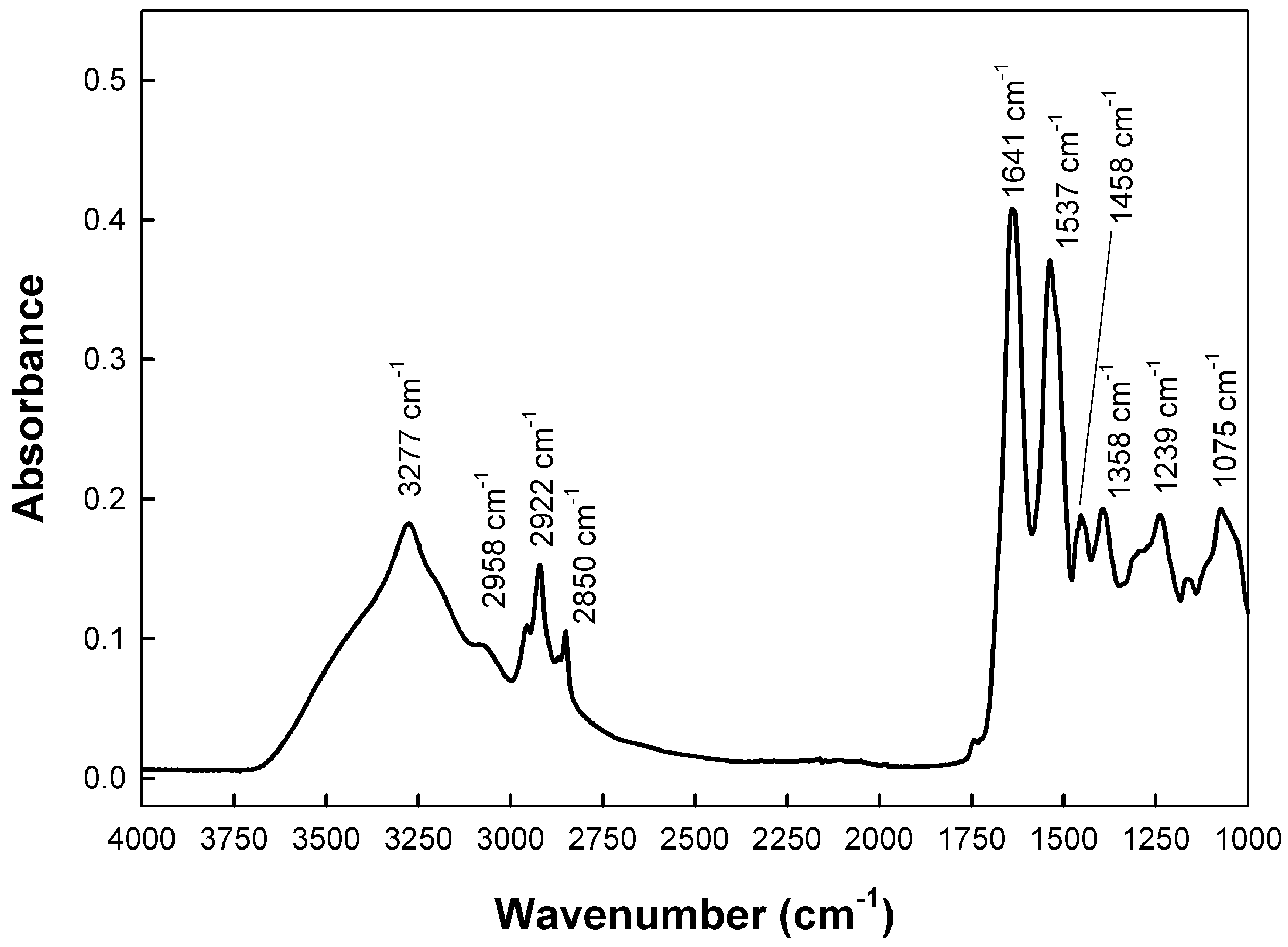
Human saliva is a heterogenous mixture of many compounds, and each component has a unique mid-infrared (mid-IR) absorption spectrum. Figure 1 shows a representative ATR-FTIR spectrum in the mid-IR region (between 4000 and 1000 cm−1), of a saliva sample deposited on paper. The major bands shown were attributed, according to previous data [35,36,37,38,39], to the following:
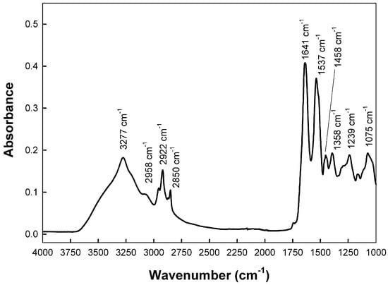
Figure 1.
A representative ATR-FTIR spectrum of a saliva sample deposited on paper indicating the maximum wavenumber of the most representative peaks in the range 4000–1000 cm−1.
- Protein Components: Amide A (~3277 cm−1), amide I (~1641 cm−1), amide II (~1543 cm−1).
- Lipid components: Acyl chains terminal methyl groups (~2956 cm−1), antisymmetric stretching of acyl chains methylene groups (~2920 cm−1), symmetric stretching of acyl chains methylene groups (~2850 cm−1), methylene groups bending (~1458 cm−1), and phospholipids (~1246 cm−1).
- Other Biomarkers: The absorption band around 1075 cm−1 corresponds to nucleic acids and phospholipids (phosphate vibrations). The band at ca. 1028 cm−1 is often attributed to glycosylated proteins and sugars.
Initial observation of the bands in Figure 1 showed that the maximum frequency of the bands stayed largely the same over time. However, the intensity of the bands generally decreased over time. This reduction in intensity suggests the deterioration of the corresponding biochemical components. Nevertheless, because direct comparisons of intensity can be misleading due to variations in sample concentration, the material’s support characteristics, or the background signal, a different approach was needed. To overcome these issues, we analyzed the ratio of intensities between specific pairs of the most relevant bands. We calculated the intensity ratios for all possible band pairs and determined their correlation coefficients. Table 1 shows the results obtained for the samples of paper indoors, which presented the most statistically significant relationships.

Table 1.
Statistically significant Pearson correlation coefficients with 95% confidence intervals between absorbance ratios and TSD for paper samples indoors.
The Pearson correlation coefficients and the statistical test were used to determine the statistical significance, which was established to 95%. Statistically relevant correlations were found for: , , , and , indicating changes in lipid acyl chains and proteins; , which correspond to proteins and phospholipids; and , monitoring changes in acyl chains methylene and terminal methyl groups. No significant correlations were found for bands corresponding to nucleic acids or sugars. Thus, it can be concluded that the time-dependent spectral changes observed were mainly due to chemical transformations involving saliva proteins and lipids. Most likely, the loss of proteins structure due to the progressive dehydration of the samples is the responsible of the changes in the amide I and amide II bands. Since albumin is the major protein in saliva, it would be reasonable to assume that these changes are mainly due to changes in albumin structure with time [36,37]. Concerning lipids, the changes found in the symmetric and antisymmetric stretching and terminal methyl stretching, most likely indicated a decrease in acyl chain mobility, probably because of changes in acyl chain length or saturation, or sample dehydration [36,37].
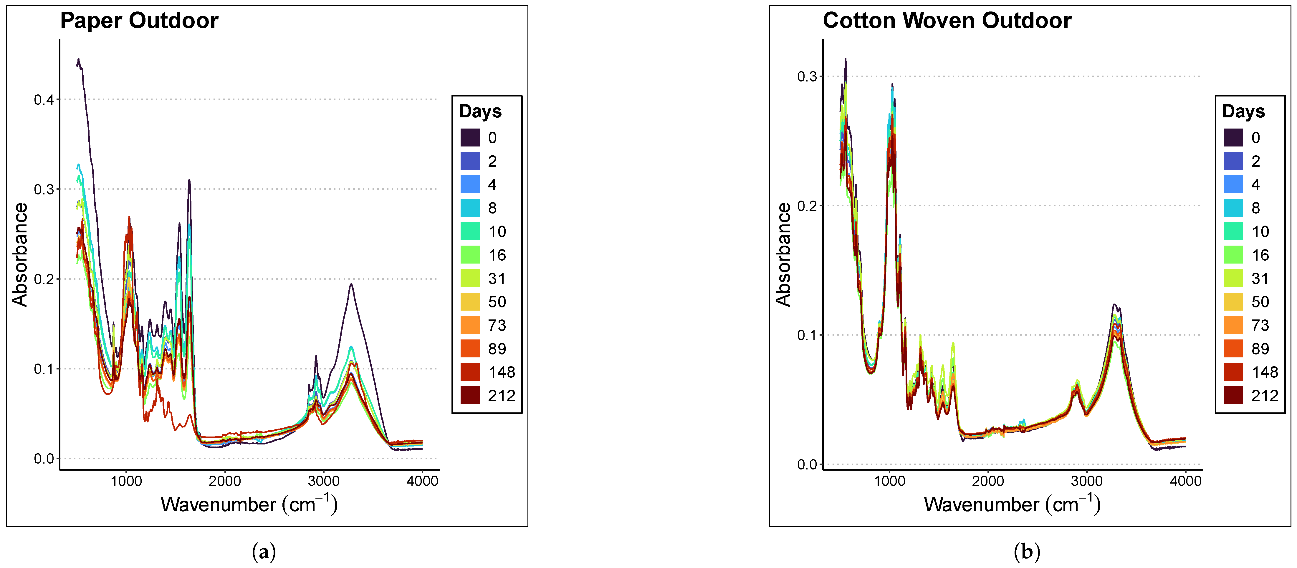
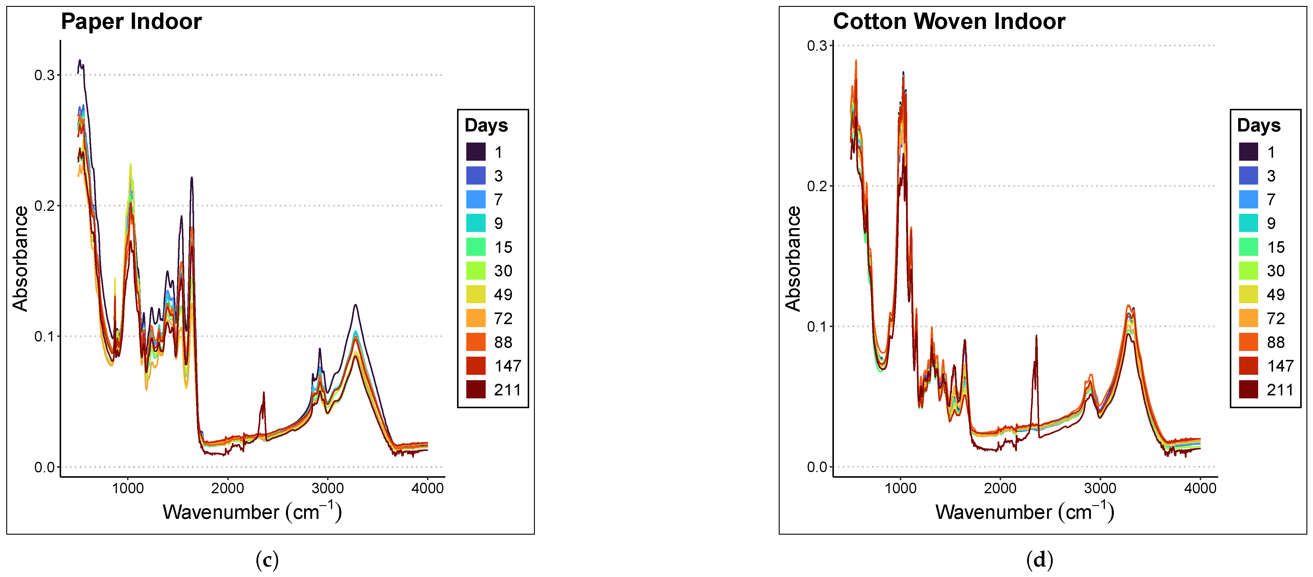
Figure 2 presents the averaged spectra of the samples at different ages within the range of 500–4000 cm−1 for each material and environmental condition considered in the study. The samples were analyzed at different time points depending on whether they were preserved indoors or outdoors; therefore, the graph legends differ. Indoor stains were analyzed at days 0, 2, 4, 8, 10, 16, 31, 50, 73, 89, 148, and 212, whereas outdoor stains were analyzed at days 1, 3, 7, 9, 15, 30, 49, 72, 88, 147, and 211. In all graphs, a subtle inverse relationship is observed between absorbance magnitude and the time since deposition; specifically, absorbance decreases as the sample ages, with the effect being more pronounced in the case of paper.
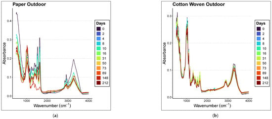

Figure 2.
Averaged spectra of the samples at different ages in the range of 500–4000 cm−1. The materials and places considered are (a) Paper Outdoor. (b) Cotton Woven Outdoor. (c) Paper Indoor. (d) Cotton Woven Indoor.
Focusing on the 1000–1800 cm−1 region of the paper spectra, panels (a) and (c) in Figure 2 show that the mean spectra corresponding to more recent samples lie above those corresponding to older ones. A less clear relationship is observed in the case of cotton woven, panels (b) and (d) in Figure 2.
Nevertheless, it is not appropriate to draw conclusions from this graphical observation, since the relationship between the spectral fingerprint and sample age must be rigorously assessed through regression models.
Once the spectra were obtained for each material and environmental condition, they were split into training and test sets with 80/20 ratio. That is, 80% of the data were used to form the training set, while the remaining 20% constituted the test set. Using the training set, a procedure was applied to select the best hyperparameters for the Savitzky–Golay filter and the optimal number of principal components for the PCR and PLS models among the values tested. The selected hyperparameters in each case are reported in Table 2.

Table 2.
Summary table of the best hyperparameters selected for each model.
These hyperparameter values were chosen following a parsimony criterion: the selected model is the simplest one whose error is less than one standard deviation away from that of the model with the lowest error. To rank models from simpler to more complex, the derivative order of the Savitzky–Golay filter and the number of principal components were used as criteria. As either of these hyperparameters increases—whether by computing a higher derivative or by selecting more principal components—the complexity of the model also increases. Therefore, Table 2 presents the models with the lowest number of principal components and lowest Savitzky–Golay derivative order whose error remains within one standard deviation of the minimum error. The window size and polynomial order are also reported in the table. However, they were not included in the selection criterion in order to simplify model ranking, and because they were found to have only a minor impact on the performance of the models. In addition, to compare the hyperparameters selected for the lowest-error model and those selected according to the parsimony criterion Table S1 is avalaible for consultation.
In all cases, applying the second derivative to the spectra using the Savitzky–Golay filter substantially improved the fit. Regarding the number of components, PLS models tended to achieve optimal performance with fewer components than PCR models, resulting in simpler models. Specifically, for PLS, six components were selected for the case of paper outdoors and for cotton woven both indoors and outdoors, while five components were selected for the case of paper indoors. In contrast, for PCR, nine components were selected for the case of paper outdoors and for cotton woven both indoors and outdoors, and seven components were selected for paper indoors.
Table 3 summarizes the error metrics obtained for each trained model using the hyperparameters selected in Table 2. Model error was evaluated under two different scenarios: cross-validation and testing. For cross-validation, only the training set was used, partitioned into folds in which some were used for training and others for error evaluation. To obtain the test metrics, each model was trained on the complete training set and its performance was then assessed on the test set, which was not involved in any stage of training. In all cases, the PLS model produced predictions that were more consistent with the true sample ages than the PCR model, leading to substantially lower errors.

Table 3.
Summary table of the goodness-of-fit of each model.
For paper stored indoors, the cross-validation RMSE obtained with the PLS model was 13.35 days compared to 23.80 days for the PCR model, a cross-validation of 0.94 versus 0.86 and a cross-validation RPIQ of 6.67 versus 3.06, respectively. A similar error trend was observed in the test set, with an RMSE of 16.54 days for PLS compared to 25.54 days for PCR, an of 0.96 versus 0.87, and an RPIQ of 4.87 versus 3.15.
Results for paper stored outdoors were similar, although the absolute differences between the mean error metrics of the models was greater in this case. In cross-validation, the PLS model achieved an RMSE of 12.64 days compared to 26.13 days for the PCR model, with values of 0.95 and 0.81, and an RPIQ of 5.59 versus 2.59, respectively. Comparable outcomes were obtained in the test set, with an RMSE of 16.54 days for PLS and 25.54 days for PCR, an of 0.96 versus 0.87, and an RPIQ of 4.87 versus 3.15.
For cotton woven stored indoors, the PLS and PCR models yielded the most similar results in terms of the absolute differences of the mean errors. In cross-validation, the PLS model obtained an RMSE of 10.04 days, an of 0.98, and an RPIQ of 7.22, compared to an RMSE of 13.24 days, an of 0.97, and an RPIQ of 5.44 for the PCR model. In the test set, PLS achieved an RMSE of 7.96 days, an of 0.99, and an RPIQ of 10.11, while PCR produced an RMSE of 15.12 days, an of 0.96, and an RPIQ of 5.32.
Finally, for cotton woven stored outdoors, the PLS model yielded, in cross-validation, an RMSE of 12.66 days, an of 0.97, and an RPIQ of 5.47, compared to an RMSE of 20.93 days, an of 0.89, and an RPIQ of 3.27 obtained with the PCR model. In the test set, the PLS model achieved an RMSE of 12.43 days, an of 0.97, and an RPIQ of 5.63, while the PCR model yielded an RMSE of 18.95 days, an of 0.92, and an RPIQ of 3.69.
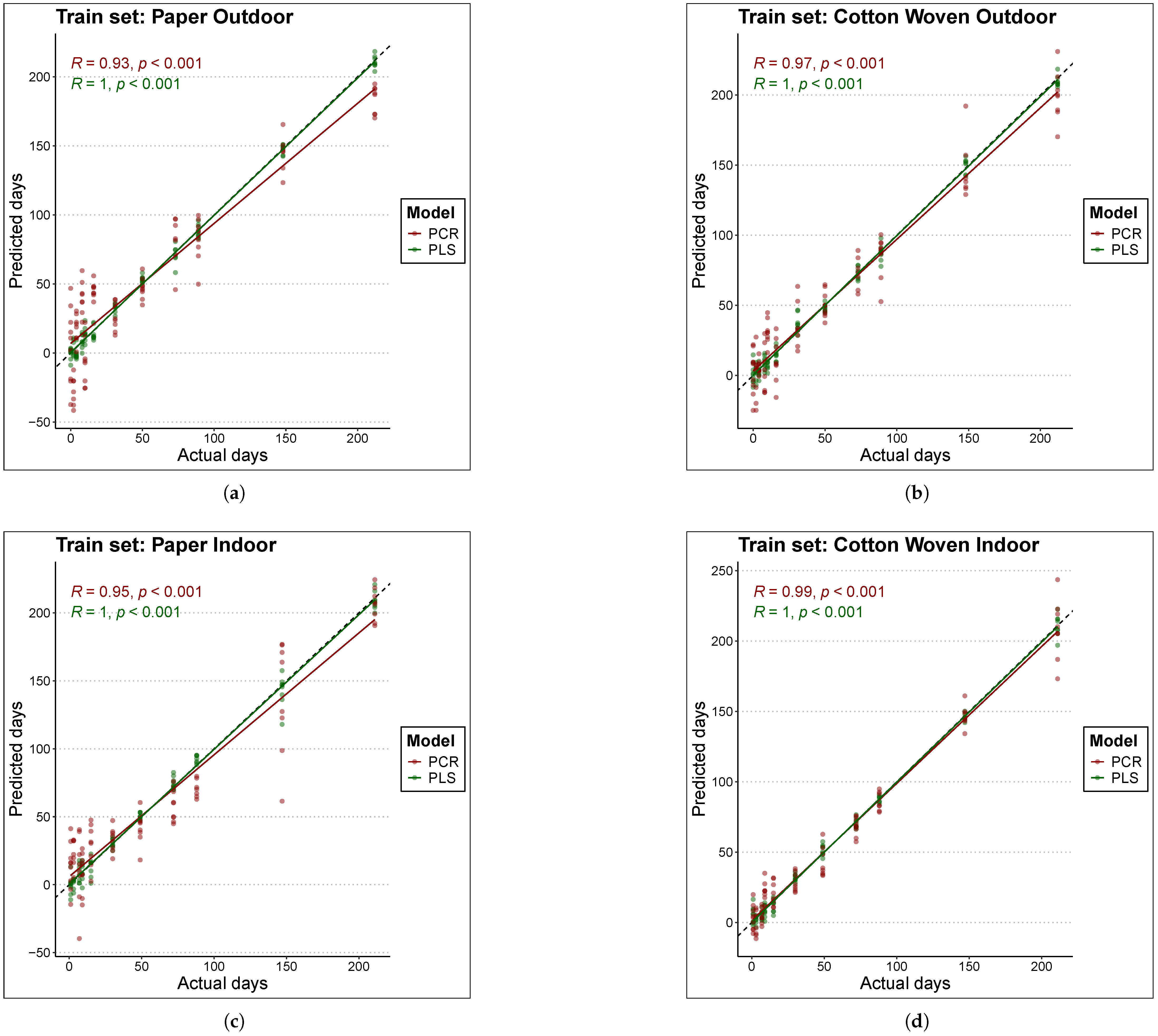
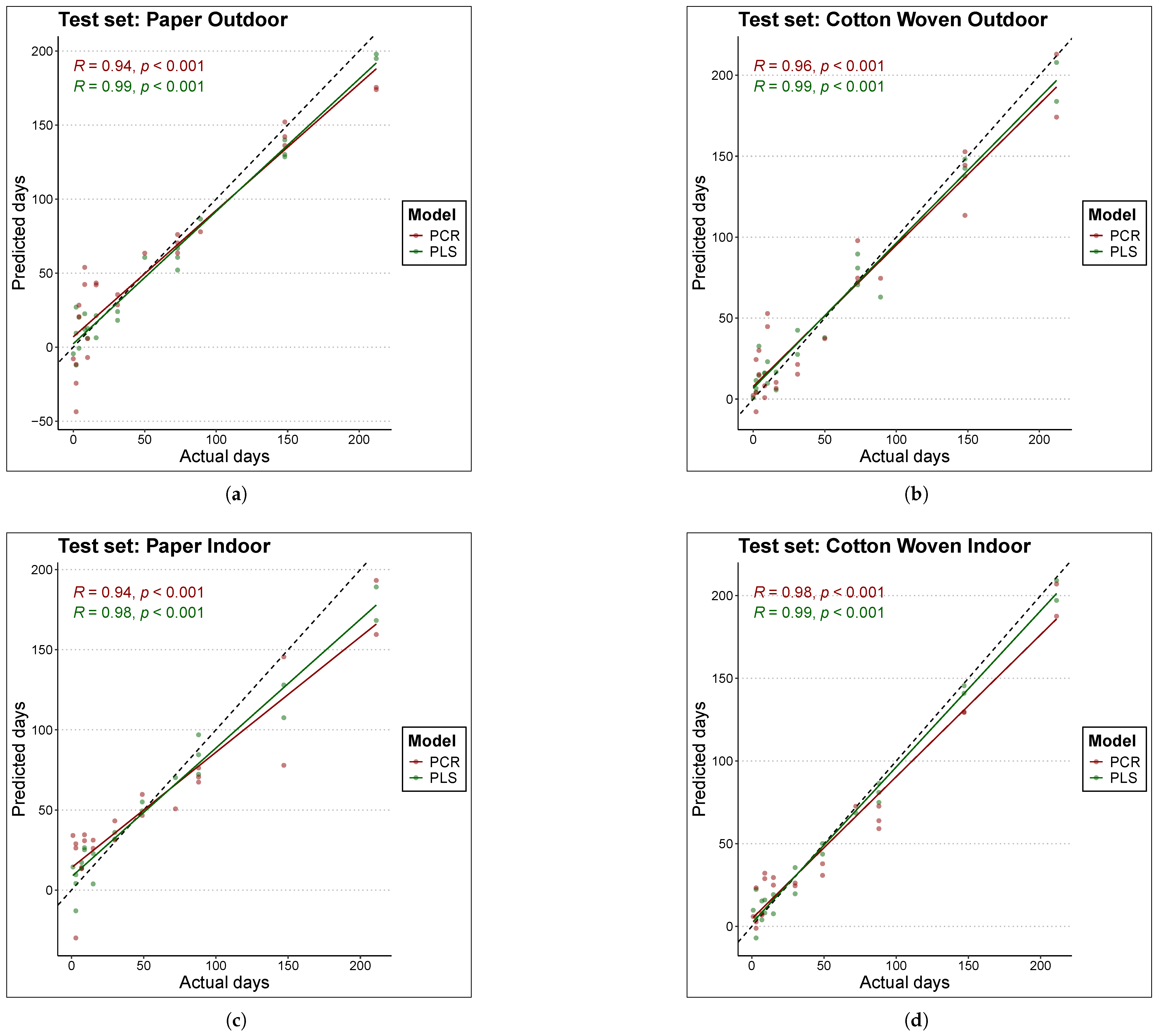
Figure 3 and Figure 4 compare the actual TSD (time since deposition) values of the samples with the predictions produced by each model. Figure 3 is based on the training data, while Figure 4 is based on the test data. Perfect fit is represented by the black line (); that is, the closer a point lies to this line, the closer the model’s TSD prediction is to the true sample value, and consequently, the lower the error. The first conclusion that clearly emerges is that, overall, PLS models estimated the true values better than PCR models, as the scatter of points is located closer to the black line in the case of PLS.
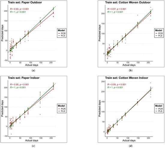
Figure 3.
Comparison of actual to predicted values for the age of train set samples with each model. The black line represents the line y = x or perfect fit. The materials and places considered are (a) Paper Outdoor. (b) Cotton Woven Outdoor. (c) Paper Indoor. (d) Cotton Woven Indoor.
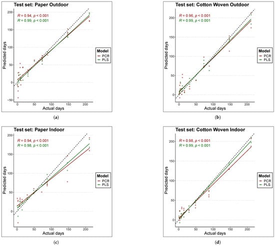
Figure 4.
Comparison of actual to predicted values for the age of test set samples with each model. The black line represents the line y = x or perfect fit. The materials and places considered are (a) Paper Outdoor. (b) Cotton Woven Outdoor. (c) Paper Indoor. (d) Cotton Woven Indoor.
For cotton woven stored indoors (panels (d) in Figure 3 and Figure 4), the scatter of points lies very close to the line. As a result, both PLS and PCR achieved the best fits in this material under this condition, in both training and test data, which is consistent with the results reported in Table 3.
On the other hand, predictions for bloodstains on paper stored indoors in the test set (panel (c) of Figure 4) with TSD values above 100 days tended to underestimate the true sample age in both models, although the effect was more pronounced for PCR. This behavior may suggest a degree of nonlinearity in the relationship between the spectral fingerprint and the sample age; however, experiments with a nonlinear model such as Support Vector Machine (SVM) did not improve the fit. A similar pattern was found for bloodstains on paper stored outdoors with the PCR model—red points in panels (a) of Figure 3 and Figure 4. In this case, the PLS model outperformed the PCR model, yielding predictions that lie closer to the line in both training and test data.
Finally, in the case of paper samples stored outdoors (panels (a) of Figure 3 and Figure 4), predictions within the range below 50 days were more consistent with the PLS model. In contrast, the PCR model exhibited a large scatter in this range, in both training and test sets, indicating that PCR failed to fully capture the pattern linking the spectral fingerprint to the sample age.
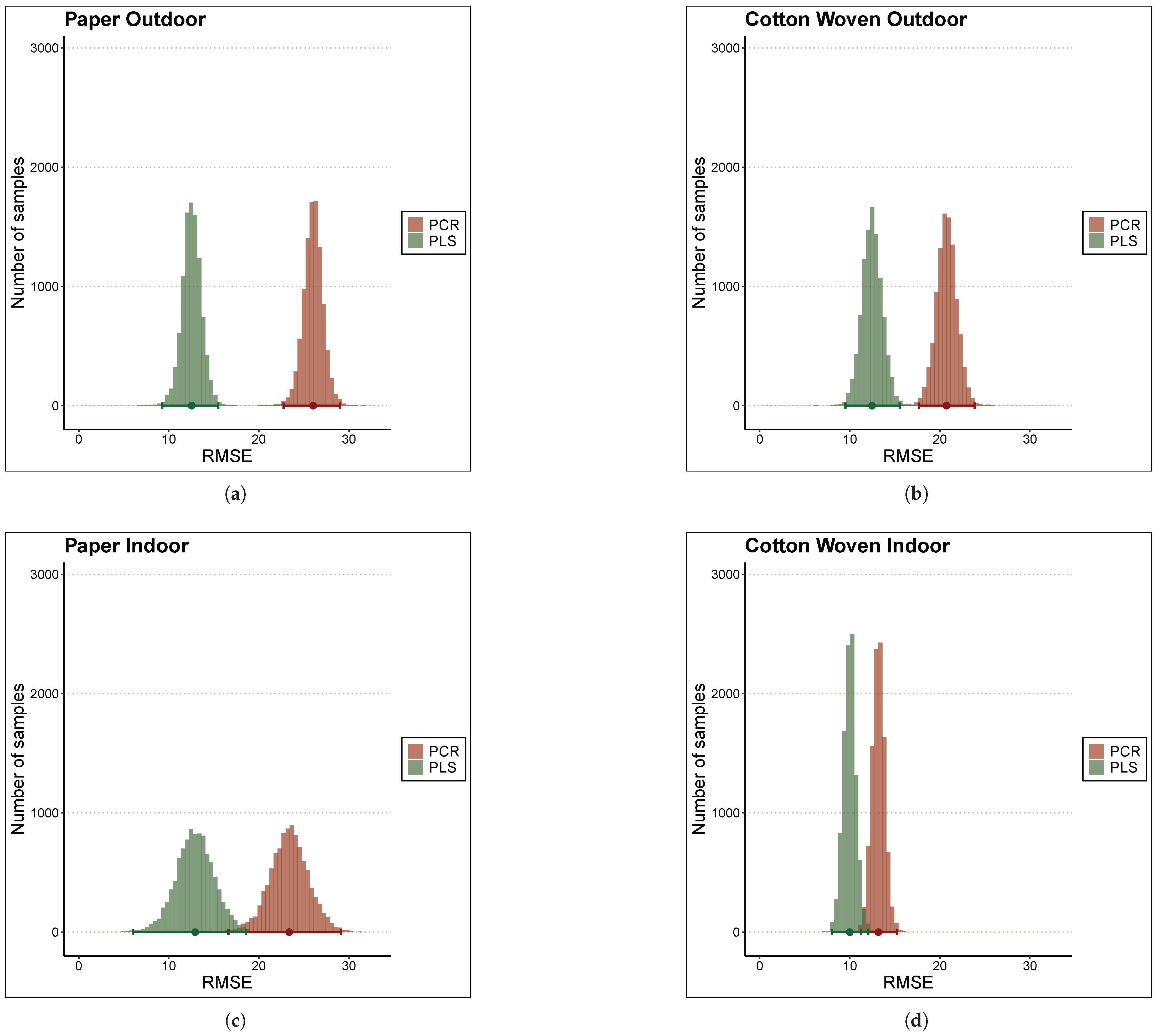
Although the error metrics in Table 3 indicate that, on average, the PLS model outperformed the PCR model, these differences could be attributed to uncontrolled random effects of the cross-validation process rather than to actual differences. To draw more consistent conclusions regarding whether this difference was statistically significant, a Bayesian linear model was fitted using a binary predictor variable indicating whether the error value was computed with PCR or PLS, the 20 RMSE values obtained via 10-fold cross-validation as the dependent variable, and an additional intercept term to model the resample-to-resample effect. All of these Bayesian linear models showed good convergence diagnostics; that is, all of them clearly converged. The posterior distributions of the RMSE for PLS and PCR under each material and environmental condition considered in the study are shown in the four panels of Figure 5.
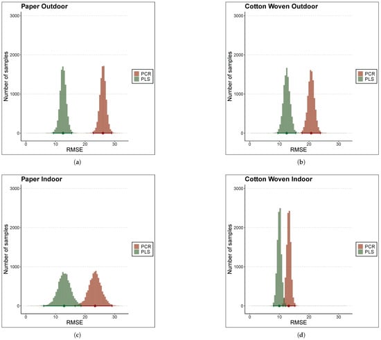
Figure 5.
Comparison of RMSE posterior distributions between PCR and PLS models via histograms of samples. The materials and places considered are (a) Paper Outdoor. (b) Cotton Woven Outdoor. (c) Paper Indoor. (d) Cotton Woven Indoor.
These plots provide a rigorous visual tool to examine differences between the models in terms of error, in this case RMSE. A greater overlap between the red and green histograms in any panel indicates greater similarity in prediction error for both models under that specific material and condition. On the other hand, the sharper the histogram, the more precise the error estimation, resulting in more reliable estimates.
For instance, RMSE values in cross-validation for paper stored indoors (panel (c)) exhibited the greatest uncertainty, as reflected in the flatter histograms. This arised from the greater heterogeneity of RMSE values across folds. At the opposite side, cotton woven stored also indoors showed the most consistent RMSE in cross-validation.
With respect to differences between models, for samples stored outdoors—both paper and cotton woven—there was virtually no overlap between histograms (panels (a) and (b)). Thus, in both cases, the PLS model consistently outperformed PCR model, particularly in the case of paper, where the difference between the histogram centers, i.e., the mean error, was substantial. On the other hand, the histograms for samples stored indoors (panels (c) and (d)) displayed a slight overlap, which can be quantified numerically by computing the credibility intervals for the mean difference in RMSE between models to assess the significance of this difference.
In Table 4, the means of the RMSE differences between the PLS and PCR models, together with their 99% credibility intervals, are reported. This table provides a numerical counterpart to Figure 5, helping to quantify the degree of overlap between histograms.

Table 4.
Summary table of differences in RMSE metric between PCR and PLS models.
According to the results, none of the intervals included zero, which means that in all cases the error of the PLS model was significantly lower than that of the PCR model with 99% credibility. Particularly noteworthy was the case of paper stored outdoors, where the PLS model improved RMSE by at least 11.73 days compared to the PCR model. This finding was consistent with what was observed in Figure 5 and with the previously discussed poor alignment of PCR predictions with the line in Figure 3 and Figure 4.
For paper stored indoors, the mean RMSE difference was 10.45 days, with the lower bound of the credibility interval at 9.39 days, indicating that the PLS model improved RMSE by at least this margin. In the case of cotton woven stored outdoors, the mean difference was 8.27 days, with a lower bound of 6.49 days. Finally, for cotton woven stored indoors, the mean difference was relatively small, of 3.19 days, as observed in Figure 5. Although the improvement of PLS over PCR in this case was statistically significant and not attributable to randomness, the magnitude of this difference was limited.
A mean error of approximately 10 days might not seem sufficient for forensic applications at this stage. However, from an operative point of view within a police context, a 10 days precision margin can be highly significative in the investigation phase, by orienting police research lines towards temporary hypotheses, or even helping to reconstruct events sequence.
4. Conclusions
The spectral changes over time found in this work are mainly due to protein and lipid degradation. The intensity of key ATR-FTIR bands decreases with time, reflecting chemical transformations associated with the loss of protein structure (especially albumin) and lipid acyl-chain mobility, likely driven by sample dehydration and other chemical processes. The PLS regression model consistently outperforms PCR in predicting the time since deposition (TSD). Across all materials and environmental conditions, PLS achieved lower RMSE, higher , and higher RPIQ values, indicating more accurate and stable predictions of sample age.
Environmental and substrate factors affect spectral stability and model performance. Applying a second derivative via the Savitzky–Golay filter improved model performance, enabling PLS and PCR to capture relevant spectral information while minimizing baseline and scattering effects. Bayesian analysis confirms the statistical significance of the performance difference between models. Posterior RMSE distributions show minimal overlap for outdoor samples, indicating a credible and consistent superiority of PLS over PCR, whereas the overlap observed for indoor samples suggests smaller yet still systematic advantages for PLS.
It should be taken into consideration that this work was intended to be an initial step toward a final viable forensic approach, which will allow a precise determination of saliva stain age under various crime situations, and not a finalized forensic protocol. Despite the fairly good results obtained in this work, it should be considered that there are certain limitations in the model mainly due to the small sample size (8 donors), which limits its generalizability. In addition, the environmental conditions simulated do not cover the wide forensic complexity that can be found in real situations (e.g., contamination, mixed fluids, humidity fluctuations). Therefore, it is planned to further extend this investigation by increasing the number of substrates and donors, testing field-portable ATR-FTIR instruments, or by comparing our models with nonlinear models (e.g., SVM, random forest, neural networks) under Bayesian optimization frameworks.
Supplementary Materials
The following supporting information can be downloaded at https://www.mdpi.com/article/10.3390/chemosensors13120409/s1, Table S1: Summary table of the hyperparameters for the model with lowest error and the model selected by the parsimony criteria. Figure S1: A representative picture of saliva stains on paper under normal and UV light.
Author Contributions
Conceptualization, M.D.P.-C. and A.O.; methodology, M.M.-P. and A.O.; software, A.J.P.-O.; validation, A.O.; formal analysis, A.J.P.-O. and M.D.P.-C.; investigation, M.M.-P. and A.O.; data curation, M.M.-P.; writing—original draft, A.O. and M.D.P.-C.; writing—review and editing, A.O. and M.D.P.-C.; visualization, A.O. All authors have read and agreed to the published version of the manuscript.
Funding
This research received no external funding.
Institutional Review Board Statement
This study was carried out according to the Declaration of Helsinki and was approved by the Committee of Ethics of the University of Murcia (protocol ID: 438/2021).
Informed Consent Statement
All the participants gave their informed consent before being included in the study.
Data Availability Statement
The original contributions presented in this study are included in the article/supplementary material. Further inquiries can be directed to the corresponding author(s).
Conflicts of Interest
The authors declare that they have no known competing financial interests or personal relationships that could have appeared to influence the work reported in this paper.
Abbreviations
The following abbreviations are used in this manuscript:
| TSD | Time Since Deposition |
| PLSR | Partial Least Squares Regression |
| PLSDA | Partial Least Squares Discriminant Analysis |
| PCA | Principal Component Analysis |
| PCR | Principal Component Regression |
| ATR-FTIR | Attenuated Total Reflectance Fourier-Transform Infrared Spectroscopy |
| RMSE | Root Mean Square Error |
| RPIQ | Ratio of Performance to Inter-Quartile |
| CI | Credibility Interval |
References
- Virkler, K.; Lednev, I.K. Blood Species Identification for Forensic Purposes Using Raman Spectroscopy Combined with Advanced Statistical Analysis. Anal. Chem. 2009, 81, 7773–7777. [Google Scholar] [CrossRef] [PubMed]
- Dziegelewski, M.; Simich, J.; Rittenhouse-Olson, K. Use of a Y Chromosome Probe as an Aid in the Forensic Proof of Sexual Assault. J. Forensic Sci. 2002, 47, 601–604. [Google Scholar] [CrossRef] [PubMed]
- Rousselet, F.; Mangin, P. Mitochondrial DNA polymorphisms: A study of 50 French Caucasian individuals and application to forensic casework. Int. J. Leg. Med. 1998, 111, 292–298. [Google Scholar] [CrossRef] [PubMed]
- Rajamannar, K. Determination of the age of bloodstains using immunoelectrophoresis. J. Forensic Sci. 1977, 22, 159–164. [Google Scholar] [CrossRef]
- Tsutsumi, A.; Yamamoto, Y.; Ishizu, H. Determination of the age of bloodstains by enzyme activities in blood cells. Nihon Hoigaku Zasshi 1983, 37, 770–776. [Google Scholar]
- Ackermann, K.; Ballantyne, K.N.; Kayser, M. Estimating trace deposition time with circadian biomarkers: A prospective and versatile tool for crime scene reconstruction. Int. J. Leg. Med. 2010, 124, 387–395. [Google Scholar] [CrossRef]
- Sampaio-Silva, F.; Magalhães, T.; Carvalho, F.; Dinis-Oliveira, R.J.; Silvestre, R. Profiling of RNA Degradation for Estimation of Post Morterm Interval. PLoS ONE 2013, 8, e56507. [Google Scholar] [CrossRef]
- Fujita, Y.; Tsuchiya, K.; Abe, S.; Takiguchi, Y.; Kubo, S.I.; Sakurai, H. Estimation of the age of human bloodstains by electron paramagnetic resonance spectroscopy: Long-term controlled experiment on the effects of environmental factors. Forensic Sci. Int. 2005, 152, 39–43. [Google Scholar] [CrossRef]
- Schweitzer, J.S.; Trombka, J.I.; Floyd, S.; Selavka, C.; Zeosky, G.; Gahn, N.; McClanahan, T.; Burbine, T. Portable generator-based XRF instrument for non-destructive analysis at crime scenes. Nucl. Instrum. Methods Phys. Res. Sect. B Beam Interact. Mater. Atoms 2005, 241, 816–819. [Google Scholar] [CrossRef]
- Strasser, S.; Zink, A.; Kada, G.; Hinterdorfer, P.; Peschel, O.; Heckl, W.M.; Nerlich, A.G.; Thalhammer, S. Age determination of blood spots in forensic medicine by force spectroscopy. Forensic Sci. Int. 2007, 170, 8–14. [Google Scholar] [CrossRef]
- Arany, S.; Ohtani, S. Age estimation of bloodstains: A preliminary report based on aspartic acid racemization rate. Forensic Sci. Int. 2011, 212, e36–e39. [Google Scholar] [CrossRef] [PubMed]
- Marrone, A.; La Russa, D.; Montesanto, A.; Lagani, V.; La Russa, M.; Pellegrino, D. Short and Long Time Bloodstains Age Determination by Colorimetric Analysis A Pilot Study. In Prime Archives in Molecular Sciences, 3rd ed.; Tarighi, S., Ed.; Vide Leaf: Hyderabad, India, 2022. [Google Scholar] [CrossRef]
- Moo, T.; Heo, S.Y.; Gwon, J.H.; Yang, S.H.; Hyun, H.G.; Sung, H.J. Hemoglobin subunit beta protein as a novel marker for time since deposition of bloodstains at crime scenes. Forensic Sci. Int. 2022, 336, 111348. [Google Scholar] [CrossRef] [PubMed]
- Das, T.; Harshey, A.; Nigam, K.; Yadav, V.K.; Srivastava, A. Analytical approaches for bloodstain aging by vibrational spectroscopy: Current trends and future perspectives. Microchem. J. 2020, 158, 105278. [Google Scholar] [CrossRef]
- Zadora, G.; Menżyk, A. In the pursuit of the holy grail of forensic science – Spectroscopic studies on the estimation of time since deposition of bloodstains. TrAC Trends Anal. Chem. 2018, 105, 137–165. [Google Scholar] [CrossRef]
- Giulietti, N.; Discepolo, S.; Castellini, P.; Martarelli, M. Neural network based hyperspectral imaging for substrate independent bloodstain age estimation. Forensic Sci. Int. 2023, 349, 111742. [Google Scholar] [CrossRef]
- Orphanou, C.M. The detection and discrimination of human body fluids using ATR FT-IR spectroscopy. Forensic Sci. Int. 2015, 252, e10–e16. [Google Scholar] [CrossRef]
- Harbison, S.; Fleming, R. Forensic body fluid identification: State of the art. Res. Rep. Forensic Med. Sci. 2016, 2016, 11–23. [Google Scholar] [CrossRef]
- Lin, H.; Zhang, Y.; Wang, Q.; Li, B.; Fan, S.; Wang, Z. Species identification of bloodstains by ATR-FTIR spectroscopy: The effects of bloodstain age and the deposition environment. Int. J. Leg. Med. 2018, 132, 667–674. [Google Scholar] [CrossRef]
- Lin, H.; Zhang, Y.; Wang, Q.; Li, B.; Huang, P.; Wang, Z. Estimation of the age of human bloodstains under the simulated indoor and outdoor crime scene conditions by ATR-FTIR spectroscopy. Sci. Rep. 2017, 7, 13254. [Google Scholar] [CrossRef]
- Hassan, N.F.N.; Sandran, D.D.; Mohamad, M.; Zakaria, Y.; Muslim, N.Z.M. Estimation of the age of bloodstains on soil matrices by ATR-FTIR spectroscopy and chemometrics. Int. J. Innov. Technol. Explor. Eng. 2019, 9, 4750–4755. [Google Scholar] [CrossRef]
- Kumar, R.; Sharma, K.; Sharma, V. Bloodstain age estimation through infrared spectroscopy and Chemometric models. Sci. Justice 2020, 60, 538–546. [Google Scholar] [CrossRef]
- Das, T.; Harshey, A.; Srivastava, A.; Nigam, K.; Yadav, V.K.; Sharma, K.; Sharma, A. Analysis of the ex-vivo transformation of semen, saliva and urine as they dry out using ATR-FTIR spectroscopy and chemometric approach. Sci. Rep. 2021, 11, 11855. [Google Scholar] [CrossRef]
- Calado, G.; Behl, I.; Byrne, H.J.; Lyng, F.M. Raman spectroscopic characterisation of non stimulated and stimulated human whole saliva. Clin. Spectrosc. 2021, 3, 100010. [Google Scholar] [CrossRef]
- Breiman, L.; Friedman, J.H.; Olshen, R.A.; Stone, C.J. Classification and Regression Trees; Wadsworth: Belmont, CA, USA, 1984. [Google Scholar]
- Bellon Maurel, V.; Fernández-Ahumada, E.; Palagos, B.; Roger, J.M.; Mcbratney, A. Critical review of chemometric indicators commonly used for assessing the quality of the prediction of soil attributes by NIR spectroscopy. TrAC Trends Anal. Chem. 2019, 29, 1073–1081. [Google Scholar] [CrossRef]
- Gabry, J.; Ben, G. Prior Distributions for Rstanarm Models, 2020. Available online: https://mc-stan.org/rstanarm/articles/priors.html (accessed on 24 November 2025).
- Kuhn, M.; Silge, J. Tidy Models with R; O’Reilly: Sebastopol, CA, USA, 2021; Chapter 11. [Google Scholar]
- R Core Team. R: A Language and Environment for Statistical Computing; R Foundation for Statistical Computing: Vienna, Austria, 2023. [Google Scholar]
- Kuhn, M.; Wickham, H. Tidymodels: A Collection of Packages for Modeling and Machine Learning Using Tidyverse Principlesl. 2020. Available online: https://www.tidymodels.org/ (accessed on 24 November 2025).
- Signal Developers. Signal: Signal Processing. Available online: https://pypi.org/project/signal/ (accessed on 24 November 2025).
- Kuhn, M. plsmod: Model Wrappers for Projection Methods. 2022. Available online: https://plsmod.tidymodels.org (accessed on 24 November 2025).
- Kuhn, M. tidyposterior: Bayesian Analysis to Compare Models Using Resampling Statistics. 2023. Available online: https://tidyposterior.tidymodels.org (accessed on 24 November 2025).
- Wickham, H. ggplot2: Elegant Graphics for Data Analysis; Springer: New York, NY, USA, 2016. [Google Scholar]
- Khaustova, S.; Shkurnikov, M.; Tonevitsky, E.; Artyushenko, V.; Tonevitsky, A. Noninvasive biochemical monitoring of physiological stress by Fourier transform infrared saliva spectroscopy. Analyst 2010, 135, 3183–3192. [Google Scholar] [CrossRef] [PubMed]
- Bel’skaya, L.V.; Sarf, E.A.; Makarova, N.A. Use of Fourier Transform IR Spectroscopy for the Study of Saliva Composition. J. Appl. Spectrosc. 2018, 85, 445–451. [Google Scholar] [CrossRef]
- Bel’skaya, L.V.; Sarf, E.A. Biochemical composition and characteristics of salivary FTIR spectra: Correlation analysis. J. Mol. Liq. 2021, 341, 117380. [Google Scholar] [CrossRef]
- Vieira, C.A.G.A.; Pupin, B.; Bhattacharjee, T.T.; Sakane, K.K. Infrared Spectroscopy Based Study of Biochemical Changes in Saliva during Maximal Progressive Test in Athletes. Anal. Sci. 2021, 37, 1157–1163. [Google Scholar] [CrossRef] [PubMed]
- Delrue, C.; De Bruyne, S.; Speeckaert, M.M. Unlocking the Diagnostic Potential of Saliva: A Comprehensive Review of Infrared Spectroscopy and Its Applications in Salivary Analysis. J. Pers. Med. 2023, 13, 907. [Google Scholar] [CrossRef]
Disclaimer/Publisher’s Note: The statements, opinions and data contained in all publications are solely those of the individual author(s) and contributor(s) and not of MDPI and/or the editor(s). MDPI and/or the editor(s) disclaim responsibility for any injury to people or property resulting from any ideas, methods, instructions or products referred to in the content. |
© 2025 by the authors. Licensee MDPI, Basel, Switzerland. This article is an open access article distributed under the terms and conditions of the Creative Commons Attribution (CC BY) license (https://creativecommons.org/licenses/by/4.0/).

