A Novel Averaging Principle Provides Insights in the Impact of Intratumoral Heterogeneity on Tumor Progression

Abstract

Typically stochastic differential equations (SDEs) involve an additive or multiplicative noise term. Here, we are interested in stochastic differential equations for which the white noise is nonlinearly integrated into the corresponding evolution term, typically termed as random ordinary differential equations (RODEs). The classical averaging methods fail to treat such RODEs. Therefore, we introduce a novel averaging method appropriate to be applied to a specific class of RODEs. To exemplify the importance of our method, we apply it to an important biomedical problem, in particular, we implement the method to the assessment of intratumoral heterogeneity impact on tumor dynamics. Precisely, we model gliomas according to a well-known Go or Grow (GoG) model, and tumor heterogeneity is modeled as a stochastic process. It has been shown that the corresponding deterministic GoG model exhibits an emerging Allee effect (bistability). In contrast, we analytically and computationally show that the introduction of white noise, as a model of intratumoral heterogeneity, leads to monostable tumor growth. This monostability behavior is also derived even when spatial cell diffusion is taken into account.

1. Introduction

The averaging theory has seen a very intense development in the last decades. Especially in the field of stochastic systems, with many applications in various branches of science, this theory has been proven revolutionary, see the work by Freidlin and Wentzell [1], the monograph by Bogoliubov and Mitropolski [2], the work by Volosov [3], the monograph by Sanders and Verhulst [4], as well as [5] for a more recent overview.

In this work, we firstly focus on an averaging principle related to random ordinary differential equations (RODEs), and then we extend it to the context of random partial differential equations (RPDEs). To start with the main idea of averaging principle we consider a dynamic system where two variables $({\rho }_t,{\xi }_t)$ coexist and interact with different time scaling; the time scaling of ${\xi }_t$ is subjected to acceleration by a factor $ϵ>0$ and so this variable becomes ${\xi }_{t/ϵ}$. In particular we assume that the slow variable ${\rho }_t$ evolves according to the following ordinary differential equation (ODE),

$$\frac{d{\rho }^{ϵ}}{dt}=F({\rho }^{ϵ},{\xi }_{t/ϵ}),{\rho }^{ϵ}\left(0\right)={\rho }_0$$

where ${\rho }_0\in \mathbb{R}$ and $F({\rho }^{ϵ},t)\in \mathbb{R}$ for each ${\rho }^{ϵ}\in \mathbb{R}.$ Averaging theory is concerned with the study of the behavior of the above ODE as $ϵ\to 0$. In particular, the averaging principle states that for $ϵ\to 0$ one can remove the fast process. More precisely, the process ${\rho }^{ϵ}$ converges to a new process $\overline{\rho }$ called averaged process and satisfies the averaged equation.

In the current work, we focus on a very particular random perturbation, given by an approximation of the white noise. The key idea of the averaging principle is explained using a model problem. Consider a non-linear dynamic system, depending on a parameter whose value is perturbed randomly. Moreover, we assume that the worst Gaussian perturbation can occur on such a parameter. In this framework, the well-posedness is not given and we will prove it using the theory of averaging. Indeed, let us consider the following ODE

$$\left\{\begin{array}{c}\frac{\partial \rho }{\partial t}=F(\rho ,k),t\in (0,T],\hfill \\ \rho \left(0\right)={\rho }_0,\hfill \end{array}\right.$$

(1)

where $F:\mathbb{R}\times \mathbb{R}\to \mathbb{R}$ is a globally Lipschitz function in terms of the solution $\rho$ of (1), as well as related to the variable $k;$ here k represents a generic parameter of the model represented by system (1). When k is a constant then the nonlinear term $F(\rho ,k)$ is well defined since $\rho$ is also the deterministic solution of the initial value problem (1).

Assume now that the parameter k is not constant but varies randomly in time, and thus some noise is integrated into system (1). One can assume that the introduced noise resembles a Gaussian process, or in a more singular case when it varies very sharply and at very short time scale, that it has the form of a white noise process. In the first case scenario, if $k\left(t\right)$ is a real valued process then system (1) is well defined and its mathematical study can be delivered through a well established theory, see [6]. On the other hand, when $k\left(t\right)$ is a white noise process, denoted by ${\xi }_t$, then we have to deal with the following system

$$\left\{\begin{array}{c}\frac{d{\rho }_t}{dt}=F(\rho ,{\xi }_t),t\in (0,T],\hfill \\ {\rho }_t\left(0\right)={\rho }_0.\hfill \end{array}\right.$$

(2)

Remarkably in system (2) the drift term is not well defined. Indeed, the drift term is a function defined on real values, whilst ${\xi }_t$ is a distribution, so it cannot serve as an argument for $F(·,·)$. The idea presented in the current work consists of substituting the white noise ${\xi }_t$ with a proper approximation, ${\xi }_t^N$, and then study the asymptotic behavior for $N\to \infty$, through the averaging theory. Intuitively speaking, ${\xi }_t^N$ are independent centered Gaussian variables with a variance that tends to be infinite. Thus, if F is a sigmoid function, with respect to the variable $\rho$, then at the limit, the average between the two extremes of the sigmoid is observed.

If the dependence on the parameter $k=k\left(t\right)$ is linear, namely

$$F(\rho ,k)=\mu \left(\rho \right)+\sigma \left(\rho \right)k,$$

the scenario changes abruptly and well-posedness is well established for the above problem. Indeed, system (1) is reduced to the following initial value problem of a stochastic differential equation (SDE)

$$\left\{\begin{array}{c}d{\rho }_t=\mu \left({\rho }_t\right)dt+\sigma \left({\rho }_t\right)d{B}_t,t\in (0,T],\hfill \\ {\rho }_t\left(0\right)={\rho }_0,\hfill \end{array}\right.$$

where $\rho ={\rho }_t$ is now a stochastic process.

The outline of the current manuscript is as follows: the next section is devoted to the biological motivation, i.e., glioma evolution. In Section 3 the white noise approximation is introduced and mathematically justified. Section 4 introduces some auxiliary results, related to the averaging approach. The following section focuses on the demonstration and the proof of our main mathematical result, the novel averaging principle: first, an averaging principle for ordinary differential equations is presented, see Theorem 1, then the result is extended to partial differential equations, see Theorem 2. In Section 6 we test the introduced averaging principle through an application related to the impact of intratumoral heterogeneity in glioma progression (see Section 2 for further biological details). It is actually observed that the introduction of randomness in the intratumoral heterogeneity works towards the disappearance of the Allee effect. Finally, we close the paper with a discussion of our main results in Section 7.

2. Biological Motivation

Two of the most important reasons for tumor treatment failure is due to intratumoral heterogeneity comprised by intrinsic and extrinsic heterogeneity [7,8]. The former describes the typically irreversible genetic or epigenetic diversity of tumor cells (e.g., due to mutations or clonal selection), and the latter is related to the reversible phenotypic responses towards microenvironmental cues usually termed as phenotypic plasticity. A well-known phenotypic plasticity phenomenon is related to the “Go or Grow” (GoG) mechanism or migration/proliferation plasticity [9], which is mainly identified in gliomas. The latter originate from glial cells in the brain and constitute the most common type of malignant brain tumor in adults [10,11]. The GoG mechanism implies a mutually exclusive switching between migratory and proliferative phenotypes. The key question is how this tumor cell decision-making mechanism is regulated, and what is its impact on tumor growth and invasion. Regarding GoG regulation, it was discovered a dependence of this cell decision mechanism on the local cell density without concluding on the exact functional form, by analyzing images of it in in vitro glioma experiments [12]. Analyzing further the potential local cell density dependencies, it was also found out low-grade tumor micro-ecology potentially exhibits an emergent Allee effect, i.e., a critical tumor cell density implying both tumor growth and control [13]. Finally, several models have shown the importance of GoG in therapy success and design [14,15,16,17].

All the aforementioned models assume that all tumor cells have an identical GoG switching mechanism. In reality, each cell may have an idiosyncratic migration and proliferation regulation, still following the GoG mechanism, due to its intrinsic heterogeneity. The question is how we can model and analyze the impact of intrinsic heterogeneity of a tumor cell population when migration and proliferation are regulated by a non-uniform GoG mechanism. In particular, we will focus on the existence of the Allee effect in the presence of intratumoral heterogeneity. To model the impact of tumor heterogeneity, we will assume a stochastic process (noise) for the GoG phenotypic switching.

To address the aforementioned questions, we need to develop a new mathematical tool that allows for the nonlinear integration of heterogeneity-induced stochasticity in the temporal evolution of the system and its corresponding analysis. An appropriate framework is offered in the context of random ordinary differential equations (RODEs). RODEs are different than stochastic differential equations (SDEs), since noise is nonlinearly integrated into the temporal evolution function of the system. Typically, averaging methods for SDEs make feasible their analysis. However, analysis of RODEs requires different tools than SDEs. To address this need, we develop a novel averaging principle allowing us to analytically draw conclusions about a tumor’s fate.

3. Mathematical Preliminaries

In the sequel some preliminaries are presented for the reader’s convenience. Throughout the manuscript, we consider random approximations of a white noise ${\left({\xi }_t\right)}_{t\in [0,T]}.$ White noise can be defined in different ways, however we will focus on the one allowing us to figure out the white noise as the “derivative” of Brownian motion. Before proceeding with the required definitions we just point out that we will work in the filtered probability space $\left(\Omega ,\mathcal{F},{\left({\mathcal{F}}_t\right)}_{t\in [0,T]},\mathbb{P}\right)$.

First, we recall the definition of a generalized Gaussian process, generalized Brownian motion and its derivative, see chapter III in [18] for further details on the theory of such process.

Definition 1.

Let us consider a generalized stochastic process Φ, namely

$$\Phi :C_c^{\infty }\left(U\right)\to L^1(\Omega ),$$

where U is an open set in $\mathbb{R}$ and $C_c^{\infty }\left(U\right)$ is the space of infinitely differentiable functions with compact support. We assume Φ to be linear and continuous. We say that Φ is a Gaussian process if for any linearly independent functions ${\varphi }_1,\dots ,{\varphi }_k\in C_c^{\infty }\left(U\right)$, the random vector $(\Phi \left({\varphi }_1\right),\dots ,\Phi \left({\varphi }_k\right))$ is normally distributed.

Notice that a Gaussian process is characterized by the following quantities: its mean

$$m_{\Phi }\left(\varphi \right):=\mathbb{E}\left[\Phi \left(\varphi \right)\right],$$

and its covariance

$$c_{\Phi }(\varphi ,\psi ):=\mathbb{E}\left\{\left[\Phi \left(\varphi \right)-m_{\Phi }\left(\varphi \right)\right]\left[\Phi \left(\psi \right)-m_{\Phi }\left(\psi \right)\right]\right\}$$

for each $\varphi ,\psi \in C_c^{\infty }\left(U\right)$.

Definition 2.

Let ${\left(B_t\right)}_{t\in {\mathbb{R}}^{+}}$ be a Brownian motion on the probability space $\left(\Omega ,\mathcal{F},{\left({\mathcal{F}}_t\right)}_{t\in [0,T]},\mathbb{P}\right).$ We consider the following generalized Gaussian process,

$$\mathcal{B}:C_c^{\infty }(0,T)\to L^2(\Omega ),$$

$$\mathcal{B}\left(\varphi \right):={\int }_0^T{\varphi }_s{B}_{s}ds,\mathrm{for}\hspace{0.17em}\mathrm{any}\varphi \in C_c^{\infty }\left(0,T\right).$$

According to the definition of derivatives of generalized Gaussian processes in [18], the derivative of the generalized Brownian motion $\mathcal{B}$ is ${\mathcal{B}}^{\prime }:\Omega \to D^{\prime }(0,T)$ and defined by

$${\mathcal{B}}^{\prime }\left(\varphi \right):=-{\int }_0^T{\varphi }_s^{\prime }{B}_{s}ds,\mathrm{for}\hspace{0.17em}\mathrm{any}\varphi \in C_c^{\infty }\left([0,T\right]).$$

Henceforth

$$\xi \left(\varphi \right)={\int }_0^T{\varphi }_s{\xi }_{s}ds:=-{\int }_0^T{\varphi }_s^{\prime }{B}_{s}ds,\mathrm{for}\hspace{0.17em}\mathrm{any}\varphi \in C_c^{\infty }\left(0,T\right).$$

(3)

Recalling that $\mathrm{cov}(B_t,B_s)=min\{t,s\}$, we can evaluate the mean and covariance of the $\xi$ as

$$m_{\xi }\left(\varphi \right)=-m_{\mathcal{B}}\left({\varphi }^{\prime }\right)=0,$$

and

$$c_{\xi }(\varphi ,\psi )={\int }_0^T{\int }_0^{T}min\{t,s\}{\varphi }_s^{\prime }{\psi }_t^{\prime }dsdt={\int }_0^T{\int }_0^T\delta (t-s){\varphi }_s{\psi }_{t}dsdt.$$

So we can conclude that the $\xi$ is a $\delta$-correlated stationary Gaussian process with mean zero and covariance $cov\left({\xi }_t{\xi }_s\right)=\mathbb{E}\left[{\xi }_t{\xi }_s\right]=\delta (t-s)$, where $\mathbb{E}$ denotes the average (expectation), see [18].

Definition 3.

The derivative of the generalized Gaussian process $\mathcal{B}$, defined in Definition 2, is denoted with ξ and it is called white noise.

As it has been already mentioned at the beginning of the section our main strategy is to work with an approximation of ${\left({\xi }_t\right)}_{t\in [0,T]}$.

Fixed $h>0$, arbitrarily small, we introduce the stochastic process ${\mathcal{B}}^h$, defined by the difference quotient of a Brownian motion, $\frac{B_{s+h}-B_s}{h}$, namely

$${\mathcal{B}}^h\left(\varphi \right):={\int }_0^T\frac{B_{s+h}-B_s}{h}{\varphi }_{s}ds\mathrm{for}\hspace{0.17em}\mathrm{any}\varphi \in C_c^{\infty }\left(0,T\right).$$

We justify our choice with the following lemma.

Lemma 1.

The process ${\mathcal{B}}^h$ converges weakly to $\xi :={\mathcal{B}}^{\prime }$, almost surely, i.e.,

$$\underset{h\to 0}{lim}{\mathcal{B}}^h\left(\varphi \right)=\xi \left(\varphi \right),\forall \varphi \in C_c^{\infty }\left([0,T]\right)a.s.$$

Proof. 

Due to the non-differentiability of Brownian motion, we first prove the result of the lemma for a mollified approximation $B_t^{\epsilon }=B_t\ast {\psi }^{ϵ}$ of Brownian motion, where ${\psi }^{\epsilon }$ is a mollifier function. It is easily seen that for any fixed $ϵ>0$ we derive

$$\begin{array}{ccc}\hfill {\mathcal{B}}^{h,\epsilon }\left(\varphi \right)={\int }_0^T\frac{B_{s+h}^{\epsilon }-B_s^{\epsilon }}{h}{\varphi }_{s}ds& & ={\int }_0^T\frac{B_{s+h}^{\epsilon }{\varphi }_{s+h}-B_s^{\epsilon }{\varphi }_s}{h}ds\hfill \\ & & -{\int }_0^T{B}_{s+h}^{\epsilon }\frac{{\varphi }_s-{\varphi }_{s+h}}{h}ds.\hfill \end{array}$$

(4)

Taking now the limit of (4) as $h\to 0$ we derive

$$\begin{array}{c}\hfill {\mathcal{B}}^{h,\epsilon }\left(\varphi \right)\underset{h\to 0}{⟶}\underset{=0}{\underbrace{{\int }_0^T{\left(B_s^{\epsilon }{\varphi }_s\right)}^{\prime }ds}}-{\int }_0^T{B}_s^{\epsilon }{\varphi }_s^{\prime }ds=-{\int }_0^T{B}_s^{\epsilon }{\varphi }_s^{\prime }ds,\end{array}$$

(5)

since $\varphi \in C_c^{\infty }(0,T).$ Notice that by dominated convergence, the following hold

$$\underset{\epsilon \to 0}{lim}{\int }_0^T{B}_s^{\epsilon }{\varphi }_s^{\prime }ds={\int }_0^T{B}_s{\varphi }_s^{\prime }ds,a.s.,$$

$$\underset{\epsilon \to 0}{lim}{\mathcal{B}}^{h,\epsilon }\left(\varphi \right)={\mathcal{B}}^h\left(\varphi \right),a.s.$$

Then, fixed $\omega \in \Omega$, and $\eta >0$, there exists ${\epsilon }_1\left(\omega \right),{\epsilon }_2\left(\omega \right),h^{\ast }\left(\omega \right)$ such that

$$\left|{\int }_0^T{B}_s^{\epsilon }{\varphi }_s^{\prime }ds-{\int }_0^T{B}_s{\varphi }_s^{\prime }ds\right|\le \frac{\eta }{3},\forall \epsilon >{\epsilon }_1,$$

(6)

$$\left|{\mathcal{B}}^{h,\epsilon }\left(\varphi \right)-{\mathcal{B}}^h\left(\varphi \right)\right|\le \frac{\eta }{3},\forall \epsilon >{\epsilon }_2,$$

(7)

$$\left|{\mathcal{B}}^{h,\epsilon }\left(\varphi \right)+{\int }_0^T{B}_s^{\epsilon }{\varphi }_s^{\prime }ds\right|\le \frac{\eta }{3},\forall h>h^{\ast }.$$

(8)

Then, from (6)–(8) we get,

$$\begin{array}{c}\left|{\mathcal{B}}^h\left(\varphi \right)-{\int }_0^T{B}_s{\varphi }_s^{\prime }\right|\le \left|{\mathcal{B}}^h\left(\varphi \right)-{\mathcal{B}}^{h,\epsilon }\left(\varphi \right)\right|+\left|{\mathcal{B}}^{h,\epsilon }\left(\varphi \right)+{\int }_0^T{B}_s^{\epsilon }{\varphi }_s^{\prime }ds\right|+\hfill \\ +\left|{\int }_0^T{B}_s^{\epsilon }{\varphi }_s^{\prime }ds-{\int }_0^T{B}_s{\varphi }_s^{\prime }ds\right|\le \frac{\eta }{3}+\frac{\eta }{3}+\frac{\eta }{3}=\eta \hfill \end{array}$$

for all $h>h^{\ast }$. We have proved that for each $\varphi \in C_c^{\infty }\left([0,T]\right)$

$$\underset{h\to 0}{lim}{\mathcal{B}}^h\left(\varphi \right)=\xi \left(\varphi \right),a.s.$$

By a standard density argument, we get that

$$\underset{h\to 0}{lim}{\mathcal{B}}^h\left(\varphi \right)=\xi \left(\varphi \right),\forall \varphi \in C_c^{\infty }\left([0,T]\right)a.s.$$

 □

We consider the process $\frac{B_{s+h}-B_s}{h}$ with $h=h_N=1/N$. Since it is continuous with respect to the variable s, we approximate it with a combination of step functions. Thus we divide the interval $[0,T]$ in small sub-intervals such that $[0,T]={\bigcup }_{i=1}^N{A}_i^N$, where $A_i^N=\left[\frac{(i-1)}{N}T,\frac{i}{N}T\right]$ with $i=1,\dots ,N$. Note that in the interval $A_i^N$ the sample is normally distributed, in particular we have

$$\frac{B_{\frac{i-1}{N}T+h_N}-B_{\frac{i-1}{N}T}}{h_N}\sim \mathcal{N}\left(0,\frac{1}{h_N}\right).$$

Consequently, inspired by Lemma 1, we consider the following random step function as an approximation of the white noise

$${\xi }_t^N=\sum _{i=𝟙}^N{\alpha }_i^N{𝟙}_{A_i^N}\left(t\right),\mathrm{where}{\alpha }_i^N=\frac{B_{\frac{i-1}{N}T+h_N}-B_{\frac{i-1}{N}T}}{h_N}\sim \mathcal{N}\left(0,N\right),$$

(9)

and ${𝟙}_{A_i^N}$ stands for the characteristic equation in $A_i^N,$ see also Figure 1.

Figure 1. In red, plot of the approximation ${\xi }_t^N$ of white noise ${\xi }_t.$

Now that one of the possible approximations of ${\xi }_t$, ${\xi }_t^N$, has been introduced, we consider ${\xi }_t^N$, instead of ${\xi }_t$, in Equation (2) and we obtain the following well-posed system, see Remark 1,

$$\left\{\begin{array}{c}\frac{d{\rho }_t^N}{dt}=F({\rho }_t^N,{\xi }_t^N\left(\omega \right)):=F_{\omega }({\rho }_t^N,t),t\in [0,T],\omega \in \Omega ,\hfill \\ {\rho }_t^N\left(0\right)={\rho }_0.\hfill \end{array}\right.$$

(10)

In particular, Equation (10) is a random ordinary differential equation (RODE), that is a non-autonomous ODE for almost every realization $\omega \in \Omega .$

The challenge is to investigate whether system (10) has a limit as $N\to \infty$ and we will do so on the specific case

$$\underset{k\to \pm \infty }{lim}F(\rho ,k)={\beta }_{\pm }\left(\rho \right)\ge 0,$$

with ${\beta }_{+}\left(\rho \right)+{\beta }_{-}\left(\rho \right)\ne 0$ for each $\rho \in \mathbb{R}.$

Intuitively speaking ${\xi }_t^N$ are independent centered Gaussian variables with variance that tends to be infinite. Our main aim is to figure out how the nonlinear term F behaves when it is perturbed by an approximation of the white noise.

4. Preliminary Results

Throughout the current manuscript we will try to implement the aforementioned ideas into system (2). Since the latter system is not well defined when the random perturbation is a white noise we will deal with the approximating system (10), where the white noise is approximated by ${\xi }_t^N,$ defined by (9), and the approximation parameter N, can be reinterpreted as the new scaling for the time variable [1]. In the current section we present some auxiliary results will be used for the proof of our novel averaging principle demonstrated and proven in Theorems 1 and 2.

We now present the main hypotheses regarding the drift F term. Henceforth, C denotes a positive constant independent of t which might change its value from line to line.

Hypothesis 1.

1. 

$F:\mathbb{R}\times \mathbb{R}\to \mathbb{R}$ is Lipschitz with respect the first variable, uniformly on the second, namely there holds

$$\left|F({\rho }_1,k)-F({\rho }_2,k)\right|\le C|{\rho }_1-{\rho }_2|,$$

(11)

for each ${\rho }_1,{\rho }_2\in \mathbb{R}$, for each $k\in \mathbb{R}$, where the positive constant C does not depends on k.

2. 

F is also bounded, i.e.,

$${\parallel F(\rho ,k)\parallel }_{\infty }\le C<+\infty .$$

(12)

3. 

F is quasi-positive with respect to ρ, that is

$$F(0,k)\ge 0.$$

(13)

4. 

Finally for each $\rho \in \mathbb{R}$ the asymptotic profile of the drift term is defined as

$$\left|F(\rho ,k)-{\beta }_{\pm }\left(\rho \right)\right|=O\left(\frac{1}{{\left|k\right|}^2}\right)\mathrm{for}k\to \pm \infty ,$$

(14)

where ${\beta }_{\pm }(·)$ are both globally Lipschitz, non-negative, and globally bounded, i.e., there exists $C_1,C_2>0$ such that

$$|{\beta }_{\pm }\left({\rho }_1\right)-{\beta }_{\pm }\left({\rho }_2\right){|}_{\infty }\le C_1|{\rho }_1-{\rho }_2|,\forall {\rho }_1,{\rho }_2\in \mathbb{R},$$

(15)

$$\parallel {\beta }_{\pm }{\left(\rho \right)\parallel }_{\infty }\le C_2<+\infty ,\forall \rho \in \mathbb{R},$$

(16)

$${\beta }_{+}\left(\rho \right)+{\beta }_{-}\left(\rho \right)\ne 0.$$

(17)

The way we interpret the solutions of RODE (10), as well as some of its features, are provided below:

Definition 4.

By a solution of the RODE (10) we mean a stochastic process such that for each realization $\omega \in \Omega$, ${\rho }_t^N\left(\omega \right)\in C\left([0,T]\right)$ and satisfies:

$${\rho }_t^N\left(\omega \right)={\rho }_0+{\int }_0^{t}F({\rho }_s^N\left(\omega \right),{\xi }_s^N\left(\omega \right))ds,$$

with a deterministic initial condition ${\rho }_0\in {\mathbb{R}}^{+}.$

Remark 1.

Since F is locally Lipschitz in its first variable, uniformly with respect to the second one, assumption (11), following a Banach fixed point argument on the space $C\left(\right[0,ϵ\left]\right)$ with some $ϵ>0$, one can prove existence and uniqueness of the solution. Then by an iterating argument, existence and uniqueness of pathwise solutions of (10) is proven for the whole interval $C\left(\right[0,T\left]\right).$ Moreover, the assumption (13) guarantees the positivity of the solutions of (10) initiated from positive initial condition ${\rho }_0\ge 0,$ see also Theorem 2.4 in [6]. The latter is a desired property in biological models like the one is considered in Section 6.

In the next section, see in particular Theorem 1, we prove that the limit towards $N\to +\infty$ of problem (10) is the following deterministic problem

$$\left\{\begin{array}{c}\frac{d\rho }{dt}=\overline{F}\left(\rho \right)\hfill \\ \rho \left(0\right)={\rho }_0,\hfill \end{array}\right.$$

(18)

where

$$0<\overline{F}\left(\rho \right)=\frac{{\beta }_{+}\left(\rho \right)+{\beta }_{-}\left(\rho \right)}{2}<\infty ,$$

(19)

due to (17).

Actually, condition (19) is considered, since we want positive solutions considering that in Section 6 we are dealing with biological populations.

Definition 5.

By a solution of the ODE (18) we mean a function $\rho \in C\left(\right[0,T\left]\right)$ satisfying:

$$\rho \left(t\right)={\rho }_0+{\int }_0^t\overline{F}\left(\rho \left(s\right)\right)ds,$$

with a deterministic initial condition ${\rho }_0\in {\mathbb{R}}^{+}.$

Remark 2.

Due to the hypothesis on $\overline{F}\left(\rho \right)$, in particular assumption (15), by standard results on ordinary differential equations, see [19], we can affirm that problem (18) and (19) admits a unique positive solution in $C\left(\right[0,T\left]\right).$

Next we deal also with the infinite dimensional case, i.e., we consider the following quasilinear partial differential equation (PDE) problem. In particular, we have a reaction–diffusion equation, where the diffusion is nonlinear but non-degenerate,

$$\begin{array}{ccc}& & \frac{\partial {\rho }_t^N}{\partial t}=\Delta \left(G\left({\rho }_t^N\right){\rho }_t^N\right)+F({\rho }_t^N,{\xi }_t^N),(x,t)\in D_T,\hfill \end{array}$$

(20)

$$\begin{array}{ccc}& & \mathcal{G}\left({\rho }_t^N\right)(x,t)=0,(x,t)\in {\Gamma }_T,\hfill \end{array}$$

(21)

$$\begin{array}{ccc}& & {\rho }_t^N(x,0)={\rho }_0\left(x\right)\ge 0,x\in D,\hfill \end{array}$$

(22)

where $D_T:=D\times (0,T),{\Gamma }_T:=\partial D\times (0,T)$ for a bounded and smooth $D\subset {\mathbb{R}}^{\ell },\ell \ge 1.$ Also, $T>0$ stands for the maximum existence time of solution ${\rho }_t^N,$ which is positive in $D_T$ as long as it exists. Here $\mathcal{G}$ is a bounded boundary operator. Besides the nonlinearities $F,G$ are both (strictly) positive and satisfy Hypothesis 1, with different constants and different limiting values ${\beta }_{\pm }.$ Solutions of problem (20)–(22) should be understood trajectorywise (pathwise) and their local existence, uniqueness and positivity can be derived by Theorem 1.1, Chapter V in [20], since (20) can be also written in divergence form as

$$\begin{array}{c}\hfill \frac{\partial {\rho }_t^N}{\partial t}=div\left({\int }_0^{{\rho }_t^N}G\left(w\right)wdw\right)+F({\rho }_t^N,{\xi }_t^N),(x,t)\in D_T.\end{array}$$

Consider now the PDE problem

$$\begin{array}{ccc}& & \frac{\partial \rho }{\partial t}=\Delta \left(\overline{G}\left(\rho \right)\rho \right)+\overline{F}\left(\rho \right),(x,t)\in D_T,\hfill \end{array}$$

(23)

$$\begin{array}{ccc}& & \mathcal{G}\rho (x,t)=0,(x,t)\in {\Gamma }_T,\hfill \end{array}$$

(24)

$$\begin{array}{ccc}& & \rho (x,0)={\rho }_0\left(x\right)\ge 0,x\in D,\hfill \end{array}$$

(25)

where $\overline{F}\left(\rho \right)$ is given by (19). Furthermore

$$\begin{array}{c}\hfill 0<\overline{G}\left(\rho \right)=\frac{g_{+}\left(\rho \right)+g_{-}\left(\rho \right)}{2}<\infty ,\end{array}$$

with $0\le g_{\pm }\left(\rho \right):={lim}_{k\to \pm \infty }G(\rho ,k)<\infty$ and $g_{-}\left(\rho \right)+g_{+}\left(\rho \right)\ne 0$ for any $\rho \in \mathbb{R}.$

Via classical parabolic theory we obtain a unique, positive solution for (23) and (25), see again Theorem 1.1, Chapter V in [20].

The rest of this section is devoted to the study of the average in time contribution (asymptotically in N) of the process ${\xi }_t^N$ on the drift term F; see Proposition 1. Before proceeding with the proof of this result we need a key tool, a law of large numbers for the random variables (r.v.) $F(x,{\alpha }_N^i),i=1,2,\dots ,N,$ which is stated and proven in the following lines.

Lemma 2.

Assume that F satisfies Hypothesis 1. For fixed $N\in \mathbb{N}$, we consider ${\alpha }_i^N\sim \mathcal{N}(0,N)$ as independent random variables, then there exists $N^{\ast }>0$ such that, for each $x\in {\mathbb{R}}^{+}$

$$\mathbb{E}{\left|\frac{1}{N}\sum _{i=1}^{N}F(x,{\alpha }_i^N)-\overline{F}\left(x\right)\right|}^4\le \frac{C}{N^{\beta }},for\hspace{0.17em}everyN>N^{\ast },$$

(26)

where $\beta >1$, $\overline{F}\left(x\right):=\frac{{\beta }_{+}\left(x\right)+{\beta }_{-}\left(x\right)}{2}>0.$

Proof. 

Define

$$S^N\left(x\right):=\frac{1}{N}\sum _{i=1}^{N}F(x,{\alpha }_i^N),$$

and ${\mu }^N{\left(x\right)}_i:=\mathbb{E}\left[F(x,{\alpha }_1^N)\right],i=1,2,\dots ,N$. Notice that ${\mu }_i^N\left(x\right)={\mu }_1^N\left(x\right)$ for all $i=1,2,\dots ,N,$ by Jensen inequality we have

$$\begin{array}{ccc}\hfill \mathbb{E}|S^N\left(x\right)-\overline{F}{\left(x\right)|}^4& & =\mathbb{E}{\left|\frac{1}{N}\sum _{i=1}^{N}F(x,{\alpha }_i^N)-\overline{F}\left(x\right)\right|}^4\hfill \\ & & =\mathbb{E}{\left|\left(\frac{1}{N}\sum _{i=1}^N\left(F(x,{\alpha }_i^N)-{\mu }^N\left(x\right)\right)\right)+\left({\mu }^N\left(x\right)-\overline{F}\left(x\right)\right)\right|}^4\hfill \\ & & \le 8·\mathbb{E}{\left|\frac{1}{N}\sum _{i=1}^N\left(F(x,{\alpha }_i^N)-{\mu }^N\left(x\right)\right)\right|}^4+8·{\left|{\mu }^N\left(x\right)-\overline{F}\left(x\right)\right|}^4\hfill \\ & & =\frac{8}{N^4}·\mathbb{E}{\left|\sum _{i=1}^N\left(F(x,{\alpha }_i^N)-{\mu }^N\left(x\right)\right)\right|}^4+8·{\left|{\mu }^N\left(x\right)-\overline{F}\left(x\right)\right|}^4.\hfill \end{array}$$

(27)

Setting $X_i:=\left(F(x,{\alpha }_i^N)-{\mu }^N\left(x\right)\right)$ the first term in the r.h.s of (27) can be expanded as

$$\begin{array}{ccc}& & \mathbb{E}\left[{\left|\sum _{i=1}^N{X}_i\right|}^4\right]\hfill \\ & & =\mathbb{E}\left[\sum _{i=1}^N{X}_i^4+\sum _{i\ne j}{X}_i^3{X}_j+\sum _{i\ne j}{X}_i^2{X}_j^2+\sum _{i_1\ne i_2\ne i_3}{X}_{i_1}{X}_{i_2}{X}_{i_3}^2+\sum _{i_1\ne i_2\ne i_3\ne i_4}{X}_{i_1}{X}_{i_2}{X}_{i_3}{X}_{i_4}\right]\hfill \\ & & =\sum _{i=1}^N\mathbb{E}\left[X_i^4\right]+\sum _{i\ne j}\mathbb{E}\left[X_i^3{X}_j\right]+\sum _{i\ne j}\mathbb{E}\left[X_i^2{X}_j^2\right]+\sum _{i_1\ne i_2\ne i_3}\mathbb{E}\left[X_{i_1}{X}_{i_2}{X}_{i_3}^2\right]\hfill \\ & & +\sum _{i_1\ne i_2\ne i_3\ne i_4}\mathbb{E}\left[X_{i_1}{X}_{i_2}{X}_{i_3}{X}_{i_4}\right].\hfill \end{array}$$

Due to the independence of the involved random variables,

$$\begin{array}{ccc}\hfill \mathbb{E}\left[{\left|\sum _{i=1}^N{X}_i\right|}^4\right]& & =\sum _{i=1}^N\mathbb{E}\left[X_i^4\right]+\sum _{i\ne j}\mathbb{E}\left[X_i^3\right]\mathbb{E}\left[X_j\right]+\sum _{i\ne j}\mathbb{E}\left[X_i^2\right]\mathbb{E}\left[X_j^2\right]\hfill \\ & & +\sum _{i_1\ne i_2\ne i_3}\mathbb{E}\left[X_{i_1}\right]\mathbb{E}\left[X_{i_2}\right]\mathbb{E}\left[X_{i_3}^2\right]+\sum _{i_1\ne i_2\ne i_3\ne i_4}\mathbb{E}\left[X_{i_1}\right]\mathbb{E}\left[X_{i_2}\right]\mathbb{E}\left[X_{i_3}\right]\mathbb{E}\left[X_{i_4}\right].\hfill \end{array}$$

Since $\mathbb{E}\left[X_i\right]=0$, the second, the fourth and the fifth sum in the above relation are equal to zero. Therefore

$$\mathbb{E}\left[{\left|\sum _{i=1}^N{X}_i\right|}^4\right]=\sum _{i=1}^N\mathbb{E}\left[X_i^4\right]+\sum _{i\ne j}\mathbb{E}\left[X_i^2\right]\mathbb{E}\left[X_j^2\right],$$

and thanks to the previous computation and to the fact that the r.v. $X_i$ are independent and identically distributed (i.i.d.) and uniformly bounded with respect to N, we obtain:

$$\begin{array}{ccc}\hfill \frac{1}{N^4}\mathbb{E}{\left|\sum _{i=1}^N{X}_i\right|}^4& & \le \frac{1}{N^4}\sum _{i=1}^N\mathbb{E}\left[X_i^4\right]+\frac{1}{N^4}\sum _{i\ne j}\mathbb{E}\left[X_i^2\right]\mathbb{E}\left[X_j^2\right]\hfill \\ & & \le \frac{N}{N^4}\mathbb{E}\left[X_1^4\right]+\frac{N·(N-1)}{N^4}\mathbb{E}{\left[X_1^2\right]}^2\hfill \\ & & \le \frac{C}{N^3}+\frac{C}{N^2}.\hfill \end{array}$$

(28)

Next we estimate the second term in the right hand side (r.h.s.) of (27). It remains to prove that

$$\left|{\mu }^N\left(x\right)-\overline{F}\left(x\right)\right|\le \frac{1}{N^{\alpha }},\mathrm{for}\mathrm{some}\alpha >\frac{1}{4}.$$

In the following it will be more convenient to rewrite ${\alpha }_i^N$ as $\sqrt{N}{Z}_i$, where $Z_i\sim \mathcal{N}(0,1)$ for $i=1,2,\dots ,N.$ Then, considering the sequence ${ϵ}_N=N^{-\gamma }$ with $\gamma \in (\frac{1}{3},\frac{3}{8})$ we have

$$\begin{array}{ccc}\hfill \left|{\mu }^N\left(x\right)-\overline{F}\left(x\right)\right|& & =\left|\mathbb{E}\left[F(x,\sqrt{N}{Z}_i)\right]-\overline{F}\left(x\right)\pm {\beta }_{+}\left(x\right)\mathbb{P}[Z_i>{ϵ}_N]\pm {\beta }_{-}\left(x\right)\mathbb{P}[Z_i>{ϵ}_N]\right|\hfill \\ & & \le \underset{\left(I\right)}{\underbrace{\left|\mathbb{E}\left[F(x,\sqrt{N}{Z}_i)\right]-({\beta }_{+}\left(x\right)+{\beta }_{-}\left(x\right))\mathbb{P}[Z_i>{ϵ}_N]\right|}}\hfill \\ & & +\underset{\left(II\right)}{\underbrace{\left|({\beta }_{+}\left(x\right)+{\beta }_{-}\left(x\right))\mathbb{P}[Z_i>{ϵ}_N]-\overline{F}\left(x\right)\right|}}.\hfill \end{array}$$

The first term, $\left(I\right)$, is estimated as follows

$$\begin{array}{c}\left|\mathbb{E}\left[F(x,\sqrt{N}{Z}_i)\right]-({\beta }_{+}\left(x\right)+{\beta }_{-}\left(x\right))\mathbb{P}[Z_i>{ϵ}_N]\right|=\hfill \\ \hspace{1em}\hspace{1em}\hspace{1em}\hspace{1em}\hspace{1em}\hspace{1em}\hspace{1em}=\underset{{\left(I\right)}_1}{\underbrace{\left|\mathbb{E}\left[F(x,\sqrt{N}{Z}_i){𝟙}_{Z_i>{ϵ}_N}\right]-{\beta }_{+}\left(x\right)\mathbb{P}[Z_i>{ϵ}_N]\right|}}\hfill \\ \hspace{1em}\hspace{1em}\hspace{1em}\hspace{1em}\hspace{1em}\hspace{1em}\hspace{1em}\hspace{1em}\hspace{1em}\hspace{1em}\hspace{1em}+\underset{{\left(I\right)}_2}{\underbrace{\left|\mathbb{E}\left[F(x,\sqrt{N}{Z}_i){𝟙}_{|Z_i|<{ϵ}_N}\right]\right|}}\hfill \\ \hspace{1em}\hspace{1em}\hspace{1em}\hspace{1em}\hspace{1em}\hspace{1em}\hspace{1em}\hspace{1em}\hspace{1em}\hspace{1em}\hspace{1em}\hspace{1em}\hspace{1em}\hspace{1em}+\underset{{\left(I\right)}_3}{\underbrace{\left|\mathbb{E}\left[F(x,\sqrt{N}{Z}_i){𝟙}_{Z_i<-{ϵ}_N}\right]-{\beta }_{-}\left(x\right)\mathbb{P}[Z_i>{ϵ}_N]\right|}},\hfill \end{array}$$

where ${\left(I\right)}_1$ can be bounded by

$$\begin{array}{c}\hfill \left|\mathbb{E}\left[F(x,\sqrt{N}{Z}_i){𝟙}_{Z_i>{ϵ}_N}\right]-{\beta }_{+}\left(x\right)\mathbb{P}[Z_i>{ϵ}_N]\right|\le \mathbb{E}\left[\left|F(x,\sqrt{N}Z)-{\beta }_{+}\left(x\right)\right|{𝟙}_{Z_i>{ϵ}_N}\right].\end{array}$$

Due to condition (14), there exists $K_0^{+}>0$ such that for each $\sqrt{K}>K_0^{+}$

$$|F(x,\sqrt{K})-{\beta }_{+}\left(x\right)|\le \frac{c}{K},$$

thus choosing N such that $\sqrt{N}{ϵ}_N>K_0^{+}$ we deduce

$$\mathbb{E}\left[\left|F(x,\sqrt{N}{Z}_i)-{\beta }_{+}\left(x\right)\right|{𝟙}_{Z_i>{ϵ}_N}\right]\le \frac{c}{N{ϵ}_N^2}\mathbb{P}[Z_i>{ϵ}_N]\le \frac{c}{N{ϵ}_N^2}.$$

Recalling that ${ϵ}_N=N^{-\gamma }$ we have that $N{ϵ}_N^2=N^{-2\gamma +1}$ and thus

$${\left(I\right)}_1\le \frac{C}{N^{-2\gamma +1}}.$$

(29)

We proceed in a very similar way to estimate ${\left(I\right)}_3,$ which again can be bounded by

$$\begin{array}{c}\hfill \left|\mathbb{E}\left[F(x,\sqrt{N}{Z}_i){𝟙}_{Z_i<-{ϵ}_N}\right]-{\beta }_{-}\left(x\right)\mathbb{P}[Z_i<-{ϵ}_N]\right|=\mathbb{E}\left[\left|F(x,\sqrt{N}Z)-{\beta }_{-}\left(x\right)\right|{𝟙}_{Z<-{ϵ}_N}\right].\end{array}$$

Again condition (14) infers the existence of some $K_0^{-}<0$ such that for each $-\sqrt{K}<K_0^{-}$ there holds

$$|F(x,-\sqrt{K})-{\beta }_{-}\left(x\right)|\le \frac{c}{K},$$

and thus by choosing N such that $-\sqrt{N}{ϵ}_N<K_0^{-}$, we obtain

$$\begin{array}{ccc}\hfill {\left(I\right)}_3& & =\mathbb{E}\left[\left|F(x,\sqrt{N}{Z}_i)-{\beta }_{-}\left(x\right)\right|{𝟙}_{Z_i<-{ϵ}_N}\right]\hfill \\ & & =\mathbb{E}\left[\left|F(x,-\sqrt{N}|Z_i\left|\right)-{\beta }_{-}\left(x\right)\right|{𝟙}_{Z_i<-{ϵ}_N}\right]\hfill \\ & & \le \frac{c}{N{ϵ}_N^2}\mathbb{P}[Z_i<-{ϵ}_N]\le \frac{c}{N^{-2\gamma +1}}.\hfill \end{array}$$

(30)

Regarding the estimation of term ${\left(I\right)}_2,$ since ${ϵ}_N=\frac{1}{N^{\gamma }}\to 0$ as $N\to \infty$ and $\mathbb{P}\left[\right|Z_i|<{ϵ}_N]=\mathrm{erf}\left(\frac{{ϵ}_N}{\sqrt{2}}\right)=O\left({ϵ}_N\right)$ we can find $N_1$ such that for $N>N_1$

$${\left(I\right)}_2=\left|\mathbb{E}\left[F(x,Z_i){𝟙}_{|Z_i|<{ϵ}_N}\right]\right|\le {\parallel F\parallel }_{\infty }\mathbb{P}\left[\right|Z_i|<{ϵ}_N]\le \frac{C}{N^{\gamma }},$$

(31)

taking also into account (12).

Additionally, term $\left(II\right)$ is estimated as:

$$\begin{array}{ccc}\hfill & & \left|({\beta }_{+}\left(x\right)+{\beta }_{-}\left(x\right))\mathbb{P}[Z_i>{ϵ}_N]-\overline{F}\left(x\right)\right|\le \left|({\beta }_{+}\left(x\right)+{\beta }_{-}\left(x\right))\right|\left|\mathbb{P}[Z_i>{ϵ}_N]-\frac{1}{2}\right|\hfill \\ & & \le \left|({\beta }_{+}\left(x\right)+{\beta }_{-}\left(x\right))\right|\left|\mathrm{erf}\left(\frac{{ϵ}_N}{\sqrt{2}}\right)\right|\le \frac{C}{N^{\gamma }}.\hfill \end{array}$$

(32)

In summary, by virtue of (29)–(32) and for $N>max\{N_1,K_0^{+},-K_0^{-}\}:=N^{\ast }$ we deduce

$$|{\mu }^N\left(x\right)-\overline{F}\left(x\right)|\le \frac{C}{N^{\alpha }},$$

where $\alpha =min\{\gamma ,1-2\gamma \}=1-2\gamma >1/4$ for $\gamma \in (\frac{1}{3},\frac{3}{8}).$ Then,

$$|{\mu }^N\left(x\right)-\overline{F}{\left(x\right)|}^4\le \frac{C}{N^{4\alpha }},$$

with $4\alpha >1$. Thus in conjunction with (28) we finally obtain the desired estimate (26).  □

Remark 3.

Lemma 2 still holds if $\frac{1}{N}{\sum }_{i=1}^{N}F(x,{\alpha }_i^N)$ is replaced by

$$\frac{1}{\alpha N}\sum _{i=1}^{\lfloor \alpha N\rfloor -k}F(x,{\alpha }_i^N),$$

with $\alpha \in (0,1]$, $k\in \mathbb{N}$. The only difference relies on the following estimate.

$$\begin{array}{c}\mathbb{E}{\left|\frac{1}{\alpha N}\sum _{i=1}^{\lfloor \alpha N\rfloor -k}F(x,{\alpha }_i^N)-\overline{F}\left(x\right)\right|}^4=\hfill \\ \hspace{1em}\hspace{1em}\hspace{1em}\hspace{1em}=\mathbb{E}{\left|\frac{1}{\alpha N}\sum _{i=1}^{\lfloor \alpha N\rfloor -k}\left(F(x,{\alpha }_i^N)-{\mu }^N\left(x\right)\right)+\frac{\lfloor \alpha N\rfloor -k}{\alpha N}{\mu }^N\left(x\right)-\overline{F}\left(x\right)\right|}^4\le \hfill \\ \hspace{1em}\hspace{1em}\hspace{1em}\le \mathbb{E}{\left|\frac{1}{\alpha N}\sum _{i=1}^{\lfloor \alpha N\rfloor -k}\left(F(x,{\alpha }_i^N)-{\mu }^N\left(x\right)\right)\right|}^4+\mathbb{E}{\left|\frac{\lfloor \alpha N\rfloor -k}{\alpha N}{\mu }^N\left(x\right)-{\mu }^N\left(x\right)\right|}^4+\hfill \\ \hspace{1em}\hspace{1em}\hspace{1em}\hspace{1em}\hspace{1em}\hspace{1em}\hspace{1em}\hspace{1em}\hspace{1em}\hspace{1em}\hspace{1em}\hspace{1em}\hspace{1em}\hspace{1em}\hspace{1em}\hspace{1em}\hspace{1em}\hspace{1em}\hspace{1em}\hspace{1em}\hspace{1em}\hspace{1em}\hspace{1em}\hspace{1em}\hspace{0.17em}\hspace{0.17em}+\mathbb{E}{\left|{\mu }^N\left(x\right)-\overline{F}\left(x\right)\right|}^4.\hfill \end{array}$$

The first and third terms are studied as in the proof of Lemma 2. By the assumption on F, (12), it is easy to see that also the second term is bounded by $\frac{C}{N^4}$.

The aim of the next pages is to prove that the sequence of solutions ${\rho }^N$ of system (10), converges to the solution $\rho$ of system (18) whose drift is given by Definition 5.

Proposition 1.

Assume that F satisfies Hypothesis 1. Let ${\xi }_t^N$ be the approximation of white noise, defined in (9), then for each $t,\mathtt{T}>0$ such that $[t,t+\mathtt{T}]\subset [0,T]$ and $x\in \mathbb{R}$ there holds

$$\underset{N\to \infty }{lim}{\int }_t^{t+\mathtt{T}}F\left(x,{\xi }_s^N\right)ds=\mathtt{T}\overline{F}\left(x\right)a.s.$$

(33)

with $\overline{F}\left(x\right):=\frac{{\beta }_{+}\left(x\right)+{\beta }_{-}\left(x\right)}{2}>0.$

Proof. 

Note that by definition (9) of the process ${\xi }_s^N$ we have

$$\begin{array}{ccc}\hfill \frac{1}{\mathtt{T}}{\int }_t^{t+\mathtt{T}}F\left(x,{\xi }_s^N\right)ds& & =\frac{1}{\mathtt{T}}{\int }_t^{t+\mathtt{T}}F\left(x,\sum _{i=1}^N{\alpha }_i^N{𝟙}_{A_i^N}\left(s\right)\right)ds\hfill \\ & & =\frac{1}{\mathtt{T}}\sum _{i=1}^{\lfloor \frac{\mathtt{T}}{T}N\rfloor }{\int }_{A_i^N\cap [t,t+\mathtt{T}]}F(x,{\alpha }_i^N)ds\hfill \\ & & =\frac{T}{\mathtt{T}}\frac{1}{N}\sum _{i=2}^{\lfloor \frac{\mathtt{T}}{T}N\rfloor -1}F(x,{\alpha }_i^N)+\frac{{\beta }_1}{\mathtt{T}}\frac{T}{N}F(x,{\alpha }_1^N)+\hfill \\ & & +\frac{{\beta }_{\lfloor \frac{\mathtt{T}}{T}N\rfloor }}{\mathtt{T}}\frac{T}{N}F(x,{\alpha }_{\lfloor \frac{\mathtt{T}}{T}N\rfloor }^N),\hfill \end{array}$$

where $\lfloor \frac{\mathtt{T}}{T}N\rfloor N$ represents the number of Gaussian variables counted in the interval $[t,t+\mathtt{T}].$ Also

$$\mathcal{L}(A_1\cap [t,t+\mathtt{T}])={\beta }_1\frac{T}{N}$$

and

$$\mathcal{L}(A_{\lfloor \frac{\mathtt{T}}{T}N\rfloor }\cap [t,t+\mathtt{T}])={\beta }_{\lfloor \frac{\mathtt{T}}{T}N\rfloor }\frac{T}{N}.$$

From the hypothesis of boundness on $F,$ (12), the last two terms on the r.h.s. converge almost surely. Next we prove that the sum ${\tilde{S}}^N\left(x\right):=\frac{T}{\mathtt{T}}\frac{1}{N}{\sum }_{i=2}^{\lfloor \frac{\mathtt{T}}{T}N\rfloor -1}F(x,{\alpha }_i^N)$ converges almost surely to $\overline{F}\left(x\right).$ To this end we can not directly apply the classical result of law of large numbers, since we are treating a triangular sequence of random variables; namely notice that r.v. $a_i^N$ depend on the double index $(i,N)$. We rewrite ${\tilde{S}}^N\left(x\right)$ by initializing the sum in $i=1$, by renaming the variables ${\alpha }_i^N$,

$${\tilde{S}}^N\left(x\right):=\frac{T}{\mathtt{T}}\frac{1}{N}\sum _{i=1}^{\lfloor \frac{\mathtt{T}}{T}N\rfloor -2}F(x,{\tilde{\alpha }}_i^N).$$

In order to prove that ${\tilde{S}}^N\left(x\right)$ converges almost surely to $\overline{F}\left(x\right)$ we equivalently demonstrate that there exists an infinitesimal sequence ${ϵ}_N$, such that

$$\mathbb{P}\left(\underset{N}{lim\; sup}{A}_N\right)=0,$$

(34)

with $A_N:=\left\{\right|{\tilde{S}}^N\left(x\right)-\overline{F}\left(x\right)|>{ϵ}_N\}$. For that purpose we appeal to Borel–Cantelli Lemma, see [21], and hence it is sufficient to show the convergence of the series ${\sum }_{N=1}^{\infty }\mathbb{P}\left(A_N\right).$ Next by virtue of Markov inequality, see [22], we derive

$$\begin{array}{ccc}\hfill \sum _{N=1}^{\infty }\mathbb{P}\left(A_N\right)& & =\sum _{N=1}^{\infty }\mathbb{P}\left(\left\{|{\tilde{S}}^N\left(x\right)-\overline{F}\left(x\right)|>{ϵ}_N\right\}\right)\hfill \\ & & =\sum _{N=1}^{\infty }\mathbb{P}\left(\left\{|{\tilde{S}}^N\left(x\right)-\overline{F}{\left(x\right)|}^4>{ϵ}_N^4\right\}\right)\hfill \\ & & \le \sum _{N=1}^{\infty }\frac{\mathbb{E}\left[|{\tilde{S}}^N\left(x\right)-\overline{F}{\left(x\right)|}^4\right]}{{ϵ}_N^4},\hfill \end{array}$$

and thus by Lemma 2 and Remark 3 we obtain

$$\sum _{N=1}^{\infty }\frac{\mathbb{E}\left[|{\tilde{S}}^N\left(x\right)-\overline{F}{\left(x\right)|}^4\right]}{{ϵ}_N^4}\le \sum _{N=1}^{\infty }\frac{1}{N^{\beta }{ϵ}_N^4}<\infty ,$$

for some $\beta >1.$ Then, under the choice ${ϵ}_N=\frac{1}{N^{\gamma }}$ with $\gamma <\frac{\beta -1}{4}$, we have that $\beta -4\gamma >1$ and consequently the convergence of the series.  □

Remark 4.

Notice that the previous statement can be reinforced in the following way. We can write that

$$\mathbb{P}\left(\underset{N\to \infty }{lim}{\int }_t^{t+\mathtt{T}}F\left(x,{\xi }_s^N\right)ds=\mathtt{T}\overline{F}\left(x\right),\forall x\in \mathbb{R}\right).$$

(35)

We consider a dense set $\mathcal{D}\subset \mathbb{R}$. From Proposition 1, we know that for each $x\in \mathcal{D}$,

$$\mathbb{P}\left(\underset{N\to \infty }{lim}{\int }_t^{t+\mathtt{T}}F\left(x,{\xi }_s^N\right)ds=\mathtt{T}\overline{F}\left(x\right)\right).$$

Since $\mathcal{D}$ is a numerable set, we can also write that

$$\mathbb{P}\left(\underset{N\to \infty }{lim}{\int }_t^{t+\mathtt{T}}F\left(x,{\xi }_s^N\right)ds=\mathtt{T}\overline{F}\left(x\right),\forall x\in \mathcal{D}\right).$$

(36)

Fixed $x\in \mathbb{R}$ there exists a subsequence $x_{n_k}$ such that ${lim}_k|x_{n_k}-x|=0$. Then

$$\begin{array}{c}\left|{\int }_t^{t+\mathtt{T}}\left(F\left(x,{\xi }_s^N\right)\left(\omega \right)-\overline{F}\left(x\right)\right)ds\right|\le \left|{\int }_t^{t+\mathtt{T}}\left(F\left(x_{n_k},{\xi }_s^N\right)\left(\omega \right)-\overline{F}\left(x_{n_k}\right)\right)ds\right|+\hfill \\ \hspace{1em}\hspace{1em}+\left|{\int }_t^{t+\mathtt{T}}\left(F\left(x,{\xi }_s^N\right)\left(\omega \right)-\overline{F}\left(x\right)\right)ds-{\int }_t^{t+\mathtt{T}}\left(F\left(x_{n_k},{\xi }_s^N\right)\left(\omega \right)-\overline{F}\left(x_{n_k}\right)\right)ds\right|\le \hfill \\ \hspace{1em}\hspace{1em}\hspace{1em}\hspace{1em}\hspace{1em}\hspace{1em}\hspace{1em}\hspace{1em}\hspace{1em}\hspace{1em}\hspace{1em}\hspace{1em}\le \left|{\int }_t^{t+\mathtt{T}}\left(F\left(x_{n_k},{\xi }_s^N\right)\left(\omega \right)-\overline{F}\left(x_{n_k}\right)\right)ds\right|+C_{\mathtt{T}}|x_{n_k}-x|.\hfill \end{array}$$

We choose k such that $|x_{n_k}-x|\le \frac{ϵ}{2C_{\mathtt{T}}}$. Moreover, for $\omega \in \tilde{\Omega }$, where $\tilde{\Omega }$ is a set of probability one, there exists $N_k^{\ast }\left(\omega \right)>0$ such that for all $N\ge N_k^{\ast }\left(\omega \right)$, the first term on the right hand side is bounded by $\frac{ϵ}{2}$. Then for all $\omega \in \tilde{\Omega }$, $\forall x\in \mathbb{R}$,

$$\underset{N\to \infty }{lim}{\int }_t^{t+\mathtt{T}}F\left(x,{\xi }_s^N,\omega \right)ds=\mathtt{T}\overline{F}\left(x\right),$$

which means that (35) is proved.

5. The Novel Averaging Principle

In the current section we present and prove our main mathematical result. Indeed, using the auxiliary results provided and proved in Section 4, we demonstrate a novel averaging principle can then be applied to the approximation (10) of system (2). As it has been already explained in the introduction the investigation of the dynamics of nonlinear system (2), under a white noise perturbation, passes through the study of the dynamics of its approximation (10) where the white noise ${\xi }_t$ is substituted by the sequence ${\xi }_t^N$ defined by (9). Then this idea can be applied, see Section 6, to study the dynamics of some nonlinear models describing the tumor growth of a brain tumor (glioblastoma).

Our first main mathematical result is stated as follows.

Theorem 1.

Let ${\xi }_t^N$ be the approximation of white noise, given by (9). Then, ${\rho }_t^N$, the solution of the RODE (10) converges uniformly in time and almost surely to ρ, the solution of the ODE (18), i.e.,

$$\underset{N\to \infty }{lim}\underset{t\in [0,T]}{sup}|{\rho }_t^N-\rho |=0a.s.$$

(37)

Proof. 

Let us take $\omega \in \Omega$. By the integral formulations of (10) and (18) we have

$$\begin{array}{ccc}\hfill {\rho }_t^N\left(\omega \right)-\rho \left(t\right)& & ={\int }_0^t[F({\rho }_s^N,{\xi }_s^N)\left(\omega \right)-\overline{F}\left(\rho \left(s\right)\right)]ds\hfill \\ & & ={\int }_0^t[F({\rho }_s^N,{\xi }_s^N)\left(\omega \right)-F(\rho \left(s\right),{\xi }_s^N)\left(\omega \right)]ds\hfill \\ & & +{\int }_0^t[F(\rho \left(s\right),{\xi }_s^N)\left(\omega \right)-\overline{F}\left(\rho \left(s\right)\right)]ds.\hfill \end{array}$$

Using the Lipschitz property (11) of the drift term F we obtain

$$\begin{array}{c}\hfill \left|{\rho }_t^N\left(\omega \right)-\rho \left(t\right)\right|\le C{\int }_0^t\left|{\rho }_s^N\left(\omega \right)-\rho \left(s\right)\right|ds+{\int }_0^t\left|F(\rho \left(s\right),{\xi }_s^N)\left(\omega \right)-\overline{F}\left(\rho \left(s\right)\right)\right|ds.\end{array}$$

Applying now Gronwall’s lemma, see [23], on the quantity $m\left(t\right)=|{\rho }_t^N-\rho \left(t\right)|\left(\omega \right)$ we derive

$$|{\rho }_t^N-\rho \left(t\right)|\left(\omega \right)\le exp\left(CT\right)\left|{\int }_0^t[F(\rho \left(s\right),{\xi }_s^N)\left(\omega \right)-\overline{F}\left(\rho \left(s\right)\right)]ds\right|,$$

and thus

$$\underset{t\in [0,T]}{sup}|{\rho }_t^N-\rho \left(t\right)|\left(\omega \right)\le exp\left(CT\right)\left|{\int }_0^T[F(\rho \left(s\right),{\xi }_s^N)\left(\omega \right)-\overline{F}\left(\rho \left(s\right)\right)]ds\right|.$$

Hence in order to prove (37) it is sufficient to show that

$$\underset{N\to \infty }{lim}\left|{\int }_0^T[F(\rho \left(s\right),{\xi }_s^N)\left(\omega \right)-\overline{F}\left(\rho \left(s\right)\right)]ds\right|=0a.s.,$$

(38)

or equivalently to demonstrate that for any fixed $\omega \in \Omega$ and for each $ϵ>0$ there exists $\overline{N}\left(\omega \right)>0$, such that for any $N>\overline{N}\left(\omega \right)$ there holds

$$\left|{\int }_0^T[F(\rho \left(s\right),{\xi }_s^N)\left(\omega \right)-\overline{F}\left(\rho \left(s\right)\right)]ds\right|\le ϵ.$$

(39)

Now we fix $ϵ$ and we discretize the interval $[0,T]$ in n sub-intervals of amplitude $\frac{T}{n},$ so we have

$$[0,T]=\bigcup _{k=0}^{n-1}\left[\frac{kT}{n},\frac{(k+1)T}{n}\right].$$

We underline the fact that the choice of n depends on $ϵ;$ that is the smaller $ϵ$ is considered then the bigger n we should choose.

Using now the above discretization we have

$$\begin{array}{ccc}\hfill {\int }_0^T\left|F(\rho \left(s\right),{\xi }_s^N)\left(\omega \right)-\overline{F}\left(\rho \left(s\right)\right)\right|ds& & =\sum _{k=0}^{n-1}{\int }_{kT/n}^{(k+1)T/n}\left|F(\rho \left(s\right),{\xi }_s^N)\left(\omega \right)-\overline{F}\left(\rho \left(s\right)\right)\right|ds\hfill \\ & & =\underset{\left({\Sigma }_1\right)}{\underbrace{{\sum }_{k=0}^{n-1}{\int }_{kT/n}^{(k+1)T/n}\left|F(\rho \left(s\right),{\xi }_s^N)\left(\omega \right)-F(\rho (kT/n),{\xi }_s^N)\right|ds}}\hfill \\ & & +\underset{\left({\Sigma }_3\right)}{\underbrace{{\sum }_{k=0}^{n-1}{\int }_{kT/n}^{(k+1)T/n}\left|F(\rho (kT/n),{\xi }_s^N)-\overline{F}\left(\rho (kT/n)\right)\right|ds}}\hfill \\ & & +\underset{\left({\Sigma }_2\right)}{\underbrace{{\sum }_{k=0}^{n-1}{\int }_{kT/n}^{(k+1)T/n}\left|\overline{F}\left(\rho (kT/n)\right)-\overline{F}\left(\rho \left(s\right)\right)\right|ds}}.\hfill \end{array}$$

(40)

We first deal with terms $\left({\Sigma }_1\right)$ and $\left({\Sigma }_2\right).$ Due to the Lipschitz property of $F,\overline{F}$ and $\rho$ we obtain

$$\begin{array}{ccc}\hfill \left({\Sigma }_1\right)+\left({\Sigma }_2\right)& & =\sum _{k=0}^{n-1}{\int }_{kT/n}^{(k+1)T/n}\left|F(\rho \left(s\right),{\xi }_s^N)\left(\omega \right)-F(\rho (kT/n),{\xi }_s^N)\right|ds\hfill \\ & & +\sum _{k=0}^{n-1}{\int }_{kT/n}^{(k+1)T/n}\left|\overline{F}\left(\rho (kT/n)\right)-\overline{F}\left(\rho \left(s\right)\right)\right|ds\hfill \\ & & \le 2C·\sum _{k=0}^{n-1}{\int }_{kT/n}^{(k+1)T/n}\left|\rho \left(s\right)-\rho (kT/n)\right|ds\hfill \\ & & \le 2C·\sum _{k=0}^{n-1}{\int }_{kT/n}^{(k+1)T/n}\left|s-kT/n\right|ds\hfill \\ & & \le 2C·\sum _{k=0}^{n-1}{\int }_{kT/n}^{(k+1)T/n}\frac{T}{n}ds\hfill \\ & & =2C·\sum _{k=0}^{n-1}\frac{T^2}{n^2}\hfill \\ & & =2C·\frac{T^2}{n}\le \frac{ϵ}{2},\hfill \end{array}$$

(41)

provided that $n>\frac{4C{T}^2}{ϵ},$ where C is a positive constant associated with the Lipschitz constants of $F,\overline{F}$ and $\rho .$

Regarding now the estimation of term $\left({\Sigma }_3\right)$, we apply Proposition 1 on each

$${\int }_{kT/n}^{kT/n+T/n}\left|F(\rho (kT/n),{\xi }_s^N)\left(\omega \right)-\overline{F}\left(\rho (kT/n)\right)\right|ds,$$

for $k=0,\dots ,n-1.$ We consider $\omega \in \tilde{\Omega }$, where $\tilde{\Omega }$ is introduced in Remark 4. Now (35) entails that for any fixed $\omega \in \tilde{\Omega }$, fixed $\frac{ϵ}{2n}$, there exists ${\overline{N}}^k\left(\omega \right)$ such that for each $N>{\overline{N}}^k\left(\omega \right)$

$${\int }_{kT/n}^{kT/n+T/n}\left|F(\rho (kT/n),{\xi }_s^N)\left(\omega \right)-\overline{F}\left(\rho (kT/n)\right)\right|ds\le \frac{ϵ}{2n}.$$

Consequently, by choosing $N>{max}_{k=1,\dots ,n-1}{\overline{N}}^k\left(\omega \right):={\overline{N}}^{ϵ}\left(\omega \right)$ we deduce

$$\left({\Sigma }_3\right)=\sum _{k=0}^{n-1}{\int }_{kT/n}^{(k+1)T/n}[F(\rho (kT/n),{\xi }_s^N)\left(\omega \right)-\overline{F}\left(\rho (kT/n)\right)]ds\le \frac{ϵ}{2}.$$

(42)

In summary, combining (41) and (42), for any fixed $\omega \in \tilde{\Omega }$ and for each $ϵ>0$ there exists $\overline{N}\left(\omega \right)$ such that (39) holds for any $N>\overline{N}\left(\omega \right)$

$${\int }_0^T\left|F(\rho \left(s\right),{\xi }_s^N)\left(\omega \right)-\overline{F}\left(\rho \left(s\right)\right)\right|ds\le ϵ,$$

and thus the proof is completed.  □

Now by using Theorem 1 in conjunction with an approach inspired by Theorem 5.16 in [24] we deduce the following infinite dimensional averaging principle. In the following we denote $H=L^2\left(D\right)$ and ${\mathcal{H}}_T=C(0,T;H).$

Theorem 2.

For every $T>0$ the unique solution ${\rho }_t^N$ of problem (20)–(22) converges as $N\to \infty$ into ${\mathcal{H}}_T$ to the unique solution ρ of the average problem (23)–(25) almost surely, i.e.,

$$\underset{N\to \infty }{lim}{\parallel {\rho }_t^N-\rho \parallel }_{{\mathcal{H}}_T}=0a.s.$$

(43)

Proof. 

For simplicity, and without loss of generality, we only provide a proof for Dirichlet boundary conditions, i.e., when $\mathcal{G}\left(w\right)=w=0$ on ${\Gamma }_T.$

Classical parabolic theory, see Theorem 2.1, Chapter V, in [20], yields that ${\rho }_t^N$ is compact in ${\mathcal{H}}_T$ and that there is a constant $C_T>0$ such that

$$\parallel {\rho }_t^N{\parallel }_{{\mathcal{H}}_T}\le C_T<+\infty ,a.s.$$

(44)

for any $T>0$.

Therefore we can find a sub-sequence, denoted again by ${\rho }_t^N$ without any confusion, and a function $\psi \in {\mathcal{H}}_T$ such that

$$\parallel {\rho }_t^N{-\psi \parallel }_{{\mathcal{H}}_T}\to 0\mathrm{a}\mathrm{s}N\to +\infty ,a.s.$$

(45)

Considering the weak formulation of (20)–(22), recalling that Dirichlet boundary conditions are considered, we have

$$\begin{array}{ccc}\hfill ⟨{\rho }_t^N,\varphi ⟩& & =⟨{\rho }_0,\varphi ⟩+⟨{\int }_0^{t}G({\rho }_{\sigma }^N,{\xi }_{\sigma }^N){\rho }_{\sigma }^{N}d\sigma ,\Delta \varphi ⟩+⟨{\int }_0^{t}F({\rho }_{\sigma }^N,{\xi }_{\sigma }^N)d\sigma ,\varphi ⟩,\hfill \end{array}$$

(46)

for any test function $\varphi \in C_0^{\infty }\left(D\right),$ where $⟨·,·⟩$ stands for the inner product in $H=L^2\left(D\right).$

After some algebraic manipulations (46) infers

$$\begin{array}{c}\hfill ⟨{\rho }_t^N,\varphi ⟩=⟨{\rho }_0,\varphi ⟩+⟨{\int }_0^{t}G({\rho }_{\sigma }^N,{\xi }_{\sigma }^N){\rho }_{\sigma }^{N}d\sigma ,\Delta \varphi ⟩-⟨{\int }_0^t\overline{G}\left({\rho }_{\sigma }^N\right){\rho }_{\sigma }^{N}d\sigma ,\Delta \varphi ⟩+\\ \hfill +⟨{\int }_0^t\overline{G}\left({\rho }_{\sigma }^N\right){\rho }_{\sigma }^{N}d\sigma ,\Delta \varphi ⟩+⟨{\int }_0^{t}F({\rho }_{\sigma }^N,{\xi }_{\sigma }^N)d\sigma ,\varphi ⟩-⟨{\int }_0^t\overline{F}\left({\rho }_{\sigma }^N\right),\varphi d\sigma ⟩\\ \hfill +⟨{\int }_0^t\overline{F}\left({\rho }_{\sigma }^N\right)d\sigma ,\varphi ⟩,\end{array}$$

and after rearrangement the preceding relation is reduced to

$$\begin{array}{c}\hfill ⟨{\rho }^N,\varphi ⟩=⟨{\rho }_0,\varphi ⟩+⟨{\int }_0^t\overline{G}\left({\rho }_{\sigma }^N\right){\rho }^{N}d\sigma ,\Delta \varphi ⟩+⟨{\int }_0^t\overline{F}\left({\rho }_{\sigma }^N\right)d\sigma ,\varphi ⟩+\end{array}$$

(47)

$$\begin{array}{c}\hfill +R_1^N\left(t\right)+R_2^N\left(t\right),\end{array}$$

(48)

where

$$\begin{array}{c}\hfill R_1^N\left(t\right):=⟨{\int }_0^t\left[\overline{G}\left({\rho }_{\sigma }^N\right)-G({\rho }_{\sigma }^N,{\xi }_{\sigma }^N)\right]{\rho }_{\sigma }^{N}d\sigma ,\Delta \varphi ⟩,\end{array}$$

and

$$\begin{array}{c}\hfill R_2^N\left(t\right):=⟨{\int }_0^{t}F({\rho }_{\sigma }^N,{\xi }_{\sigma }^N)-\overline{F}\left({\rho }_{\sigma }^N\right)d\sigma ,\varphi ⟩.\end{array}$$

We now consider a discretization of the interval $[0,T]$ in n subintervals of amplitude $\frac{T}{n},$ so we have

$$[0,T]=\bigcup _{k=0}^{n-1}\left[\frac{kT}{n},\frac{(k+1)T}{n}\right],$$

and we introduce a step function, ${\rho }_t^{N,n}$, which is a discretized version of the function ${\rho }_t^N$,

$${\rho }_s^{N,n}=\sum _{k=0}^{n-1}{\rho }_{\frac{kT}{n}}{𝟙}_{\left[\frac{kT}{n},\frac{(k+1)T}{n}\right)}\left(s\right).$$

Then, we rewrite the first $R_1^N\left(t\right)$ as

$$\begin{array}{cc}\hfill ⟨{\int }_0^t[G({\rho }_{\sigma }^N,{\xi }_{\sigma }^N)-\overline{G}\left({\rho }_{\sigma }^N\right)]{\rho }_{\sigma }^{N}d\sigma ,\varphi ⟩& =⟨{\int }_0^{t}G({\rho }_{\sigma }^N,{\xi }_{\sigma }^N){\rho }_{\sigma }^N-G({\rho }_{\sigma }^{N,n},{\xi }_{\sigma }^N){\rho }_{\sigma }^{N,n}d\sigma ,\varphi ⟩\hfill \\ \hfill & +⟨{\int }_0^{t}G({\rho }_{\sigma }^{N,n},{\xi }_{\sigma }^N){\rho }_{\sigma }^{N,n}-\overline{G}\left({\rho }_{\sigma }^{N,n}\right){\rho }_{\sigma }^{N,n}d\sigma ,\varphi ⟩\hfill \\ \hfill & +⟨{\int }_0^t\overline{G}\left({\rho }_{\sigma }^{N,n}\right){\rho }_{\sigma }^{N,n}-\overline{G}\left({\rho }_{\sigma }^N\right){\rho }_{\sigma }^{N}d\sigma ,\varphi ⟩.\hfill \end{array}$$

(49)

First, we observe that due to the parabolic regularity, cf. Theorem 2.1, Chapter V, in [20], for some $C,C_1>0$

$$\parallel {\rho }_t^N-{\rho }_s^N{\parallel }_{L^2\left(D\right)}\le C|t-s|.$$

$$\parallel {\rho }_t^N{\parallel }_{L^{\infty }([0,T],L^2\left(D\right))}\le C_1.$$

We thus estimate the first and third terms on the right hand side of (49) by Hölder inequality and by assumption (11) and choosing n big enough we derive

$$\begin{array}{cc}\hfill ⟨{\int }_0^{t}G({\rho }_{\sigma }^N,{\xi }_{\sigma }^N){\rho }_{\sigma }^N-G({\rho }_{\sigma }^{N,n},{\xi }_{\sigma }^N){\rho }_{\sigma }^{N,n}d\sigma ,\varphi ⟩& +⟨{\int }_0^t\overline{G}\left({\rho }_{\sigma }^{N,n}\right){\rho }_{\sigma }^N-\overline{G}\left({\rho }_{\sigma }^N\right){\rho }_{\sigma }^{N,n}d\sigma ,\varphi ⟩\le \hfill \\ \hfill & \le C_{\varphi ,G}{\int }_0^t{\parallel {\rho }_{\sigma }^N-{\rho }_{\sigma }^{N,n}\parallel }_{L^2\left(D\right)}\hfill \\ \hfill & \le C_{\varphi ,G}\sum _{k=0}^{n-1}{\int }_{kt/n}^{(k+1)t/n}{\parallel {\rho }_{\sigma }^N-{\rho }_{\frac{kT}{n}}^N\parallel }_{L^2\left(D\right)}\le \hfill \\ \hfill & \le C_{\varphi ,G}\frac{t^2}{n}\le \frac{ϵ}{2},\hfill \end{array}$$

for some $ϵ>0$.

Regarding the second term on the right hand side of (49),

$$\begin{array}{ccc}& & ⟨{\int }_0^t[G({\rho }_{\sigma }^{N,n},{\xi }_{\sigma }^N)-\overline{G}\left({\rho }_{\sigma }^{N,n}\right)]{\rho }_{\sigma }^{N,n}d\sigma ,\varphi ⟩\hfill \\ & & =\sum _{k=0}^{n-1}{\int }_D\left({\int }_{kt/n}^{(k+1)t/n}G({\rho }_{\frac{kT}{n}}^N\left(x\right),{\xi }_{\sigma }^N)-\overline{G}\left({\rho }_{\frac{kT}{n}}^N\left(x\right)\right)d\sigma \right){\rho }_{\frac{kT}{n}}^N\left(x\right)\varphi \left(x\right)dx\hfill \\ & & \le \sum _{k=0}^{n-1}{\left({\int }_D{\left({\int }_{kt/n}^{(k+1)t/n}G({\rho }_{\frac{kT}{n}}^N\left(x\right),{\xi }_{\sigma }^N)-\overline{G}\left({\rho }_{\frac{kT}{n}}^N\left(x\right)\right)d\sigma \right)}^2\varphi {\left(x\right)}^{2}dx\right)}^2{\parallel {\rho }_t^N\parallel }_{{\mathcal{H}}_T}.\hfill \end{array}$$

By Proposition 1 and Remark 4 we have that

$$\underset{N\to \infty }{lim}\left({\int }_{kt/n}^{(k+1)t/n}G({\rho }_{\frac{kT}{n}}^N\left(x\right),{\xi }_{\sigma }^N)-\overline{G}\left({\rho }_{\frac{kT}{n}}^N\left(x\right)\right)d\sigma \right)=0,\forall x\in D,a.s.$$

Since this term is also bounded in $L^{\infty }\left(D\right)$ and due to (44), we can conclude by dominated convergence that also the space integral converges as well. In particular, there exists $N_k>0$ such that for all $N>N_k$

$$\left|{\int }_D\left({\int }_{kt/n}^{(k+1)t/n}G({\rho }_{\frac{kT}{n}}^N\left(x\right),{\xi }_{\sigma }^N)-\overline{G}\left({\rho }_{\frac{kT}{n}}^N\left(x\right)\right)d\sigma \right)\varphi \left(x\right)dx\right|\le \frac{ϵ}{2n}.$$

Then for all $N>N^{\ast }:={max}_k{N}_k$,

$$\left|⟨{\int }_0^{t}G({\rho }_{\sigma }^{N,n},{\xi }_{\sigma }^N)-\overline{G}\left({\rho }_{\sigma }^{N,n}\right)d\sigma ,\varphi ⟩\right|\le \frac{ϵ}{2}.$$

In other terms, we have proved that

$$\begin{array}{c}\hfill R_1^N\left(t\right)\to 0\mathrm{a}\mathrm{s}N\to +\infty \mathrm{for}\hspace{0.17em}\mathrm{any}0<t<T,a.s.\end{array}$$

(50)

Following a similar argument, we can also prove that

$$\begin{array}{c}\hfill R_2^N\left(t\right)\to 0\mathrm{a}\mathrm{s}N\to +\infty \mathrm{for}\hspace{0.17em}\mathrm{any}0<t<T,a.s.\end{array}$$

(51)

Letting now $N\to +\infty$ into (47) and using (50) and (51), we derive

$$\begin{array}{ccc}\hfill ⟨\psi ,\varphi ⟩& & =⟨{\rho }_0,\varphi ⟩+⟨{\int }_0^t\overline{G}\left(\psi \right)\psi d\sigma ,\Delta \varphi ⟩+⟨{\int }_0^t\overline{F}\left(\psi \right)d\sigma ,\varphi ⟩,\hfill \end{array}$$

i.e., $\psi$ is a weak solution of (20)–(22). However, this problem has a unique weak solution, cf. Theorem 6.6., Chapter V, in [20], so we finally infer that $\psi =\rho .$ This completes the proof of the Theorem.  □

6. Application: Impact of Intratumoral Heterogeneity in Glioma Progression

The main purpose of the current section is to apply the averaging principle, as introduced in Theorems 1 and 2, to address the problem of intrinsic heterogeneity in glioma progression.

6.1. The Go or Grow Model of Glioma

For the reader’s convenience, we briefly present the derivation of the “Go or Grow” model, as introduced by Hatzikirou et al. [9]. Due to the migration/proliferation dichotomy, we can distinguish the total population of glioma cells $\rho$ in two groups, ${\rho }^p$ proliferating cells and ${\rho }^m$ migratory cells. For each type of population we can then write down a mean-field equation (the original system was a stochastic cellular automaton) describing the corresponding dynamics, so we have the following system, which is described as the classical GoG model,

$$\begin{array}{ccc}\hfill \frac{\partial {\rho }^m}{\partial t}& & =\Delta {\rho }^m+r_{p\to m}\left(\rho \right){\rho }^p-r_{m\to p}\left(\rho \right){\rho }^m-r_d{\rho }^m,\hfill \end{array}$$

(52)

$$\begin{array}{ccc}\hfill \frac{\partial {\rho }^p}{\partial t}& & =r_b{\rho }^p(1-{\rho }^p)+r_{m\to p}\left(\rho \right){\rho }^m-r_{p\to m}\left(\rho \right){\rho }^p-r_d{\rho }^p,\hfill \end{array}$$

(53)

where $r_b$ is the birth rate, $r_d$ is the death rate, $r_{p\to m}\left(\rho \right)$ is the switch rate from proliferating to motile phenotype, and $r_{m\to p}\left(\rho \right)$ is the switch rate from motile to proliferating phenotype of the tumor cells. Please note that we hypothesize that the phenotypic switch between proliferative and migratory phenotypes depends on the local cell density. We regard variations in the local cell density as the result of tumor cell interactions with extracellular matrix components, chemical cues, and other stromal cells. Therefore, we model the impact of the aforementioned factors by means of their impact on cell density.

To obtain a unique equation for $\rho ={\rho }^m+{\rho }^p$, we refer to the time scale separation between intracellular processes and cell level ones. The former corresponds to the decision of the cell between “Go or Grow” states which is dictated by the underlying intracellular signaling pathway activation (typically this is at the time scale of minutes). On the other hand, although cell decision is quite fast, the execution characteristic time of these cell process are much slower. Cell proliferation typically takes 24 h and cell migration is at the order of magnitude of 1 h (it involves many processes such as the creation of focal adhesion point, polymerization of the cytoskeleton, extension of pseudopodia, and retraction). For further details one could read the published studies [15,17,25]. Therefore, we can assume that the exchange term is at a quasi-equilibrium state satisfying the following:

$${\rho }^p{r}_{p\to m}\left(\rho \right)={\rho }^m{r}_{m\to p}\left(\rho \right).$$

Through this condition we can rewrite the preceding system as a single PDE (details of the calculation can be found in [13])

$$\frac{\partial \rho }{\partial t}=\Delta \left(r_{p\to m}\left(\rho \right)\rho \right)+r_b{r}_{m\to p}\left(\rho \right)\rho (1-\rho )-r_d\rho .$$

(54)

The phenotypic switching is regulated by local microenvironmental cues, being lumped into local density dependence. For the sake of simplicity, we will assume that both switching rates, $r_{p\to m}\left(\rho \right)$ and $r_{m\to p}\left(\rho \right)$, depend monotonously on cell density, approximated by a sigmoid function with slope parametrized by k. Intuitively, the slope can be viewed as the way that single tumor cell interprets its microenvironment and decides over its phenotype. The parameter $\theta$ represents the critical cell density value at which the probabilities of switching from one phenotype into the other are the same. Following [13], we consider that the two rates are complementary, namely if cell motility increases with cell density then cell proliferation decreases with density and vice versa: namely if k denotes the slope of the switch from motile type to proliferating type, then $-k$ denotes the slope of the switch from proliferating type to motile type. A possible choice is given by the following, see also Figure 2,

$$\begin{array}{ccc}\hfill r_{m\to p}\left(\rho \right)& & =\frac{1}{2}\left(1+tanh\left(k\right(\rho -\theta \left)\right)\right):=r_s\left(\rho \right),\hfill \end{array}$$

(55)

$$\begin{array}{ccc}\hfill r_{p\to m}\left(\rho \right)& & =1-r_s\left(\rho \right),\hfill \end{array}$$

(56)

and thus (54) takes the form

$$\frac{\partial \rho }{\partial t}=\Delta \left((1-r_s(\rho ,k))\rho \right)+r_b{r}_s(\rho ,k)\rho (1-\rho )-r_d\rho .$$

(57)

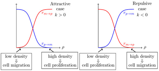
Figure 2. Sketch of cellular mechanism for different kind of phenotypic plasticity. In the left aggregative configuration is represented, while in the right figure, the repulsive configuration is represented.

For positive slope $k>0$ the phenotypic switch presents an attractive behavior, while for $k<0$ a repulsive one (see Figure 2) [13]. To the best of our knowledge the GoG model (57) has been only investigated for the case when k is a constant, see [13], i.e., the tumor cell population decides in a homogeneous way overproliferation or migration. Here we assume that tumor is heterogeneous in the way cells regulate their migration/proliferation phenotype controlled by a stochastic parameter $k.$

6.2. Intrinsic Intratumoral Heterogeneity of Glioma Cells as a White Noise

We recall that the sign of k indicates the regime where we locate in; it actually identifies if we are in an attractive or repulsive regime, whilst the absolute value of k measures the intensity of the phenotypic switching. In the following, we introduce the desirable heterogeneous regulation of the switch by assuming that k follows a probability distribution, i.e., we heuristically take

$$k\mapsto k+\mathrm{Noise}.$$

(58)

It is anticipated that the introduced intrinsic heterogeneity facilitates the tumor growth and persistence [7,8]. Therefore it is plausible to consider the “worst” case heterogeneity scenario, hence the distribution of k resembles that of white noise. As a first step towards the investigation of the dynamics of the GoG model (57) under the random perturbation (58), we choose to neglect the contribution of the diffusion, and thus we initially consider the following ODE

$$\left\{\begin{array}{c}\frac{\partial \rho }{\partial t}=F(\rho ,k):=r_b{r}_s(\rho ,k)\rho (1-\rho )-r_d\rho ,\hfill \\ 0\le \rho \left(0\right)={\rho }_0\le 1,\hfill \end{array}\right.$$

(59)

where $r_s(\rho ,k)$ given by (55) for $r_b>r_d$, $\theta \in [0,1]$ and ${\rho }_0\in {\mathbb{R}}^{+}.$

If one wants to approximate k as a white noise, clearly relapses in the case demonstrated in Section 1, since the occurring system

$$\left\{\begin{array}{c}\frac{\partial {\rho }^{\xi }}{\partial t}=F(\rho ,\xi ),\hfill \\ 0\le \rho \left(0\right)={\rho }_0\le 1,\hfill \end{array}\right.$$

(60)

is not well defined as was also explained in the Introduction.

In order to tackle system (60) we appeal to the averaging principle demonstrated by Theorem 1. To this end we just need to verify all the involved conditions of Hypothesis 1. We first note that condition (11) is trivially verified, since the drift term $F(\rho ,k)=r_b{r}_s(\rho ,k)\rho (1-\rho )-r_d\rho$ for $\rho \in [0,1]$ is differentiable. Besides F is bounded on both variables $(\rho ,k)$, since k appears as an argument of the hyperbolic tangent, and the variable $\rho$ varies in a compact set. Thus condition (12) also holds. Obviously we have $F(0,k)=0$ and thus condition (13) is fulfilled too. It remains to check the validity of condition (14). It can be easily seen that

$$\underset{k\to \pm \infty }{lim}\left(r_b{r}_s(\rho ,k)\rho (1-\rho )-r_d\rho \right)=r_b{\beta }_{\pm }\rho (1-\rho )-r_d\rho ,$$

with ${\beta }_{\pm }=\{1,0\}$ where the order of convergence is exponential, and hence condition (14) is also satisfied. Consequently we have the following, as a straightforward consequence of Theorem 1.

Theorem 3.

Let ${\xi }_t^N$ be the process described by (9).Then the solution trajectories ${\rho }_t^N$ of

$$\left\{\begin{array}{c}\frac{\partial {\rho }^N}{\partial t}=r_b{r}_s({\rho }^N,{\xi }^N){\rho }^N(1-{\rho }^N)-r_d{\rho }^N,\hfill \\ 0\le \rho \left(0\right)={\rho }_0\le 1,\hfill \end{array}\right.$$

(61)

converge uniformly in time and almost surely to the solution trajectories ρ of the following ODE problem

$$\left\{\begin{array}{c}\frac{\partial \rho }{\partial t}=\frac{1}{2}{r}_b\rho (1-\rho )-r_d\rho \hfill \\ 0\le \rho \left(0\right)={\rho }_0\le 1.\hfill \end{array}\right.$$

(62)

Namely,

$$\underset{N\to \infty }{lim}\underset{t\in [0,T]}{sup}|{\rho }_t^N-\rho \left(t\right)|=0a.s.$$

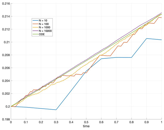
In particular, if one wishes to investigate the stability of the random model (61) then Theorem 3 provides the relevant approximating ODE (62) which should be analyzed in order to have a qualitative behaviour of glioblastoma’s growth. The visualization of the result of Theorem 3 can be seen in Figure 3.

Figure 3. Plot of sample trajectories of ${\rho }_t^N$, solution of equation (61), for different values of N, in green the trajectory of the solution of the deterministic ODE (62).

Let us here recall that in the absence of intrinsic heterogeneity, the trivial solution ${\rho }_{nc}=0$ is a stable point for a certain range of parameters, as shown in [13], see also Figure 4However, under the assumption of white noise intrinsic heterogeneity, the stability analysis of (62) leads to a configuration that is monostable under some reasonable assumptions. Indeed, if $r_b>2r_d$ the point ${\rho }_c=1-2\frac{r_d}{r_b}$ is the only stable point, whilst ${\rho }_{nc}=0$ is still a fixed point but unstable (see Figure 5). When $r_b<2r_d$, we have a predictable result, considering the fact that the death rate is bigger than the birth rate: ${\rho }_{nc}=0$ is the only stable point, and moreover is also the only fixed point in the range $\rho \in [0,1]$. In this case, the parameters $(k,\theta )$ do not influence the model’s steady states as in the deterministic case, see again Figure 4. Consequently, the strength of the white noise is so large that it annihilates the existence of multiple steady states. Finally, the Allee effect that was observed in the deterministic case [13] now disappears and the remaining effect is the survival of the steady cancerous population.

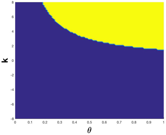
Figure 4. Allee effect in the deterministic system (59): The yellow area represents the area where 0 is stable for this system, whereas the blue one depicts the area where 0 becomes unstable.

Figure 5. Plot of $\overline{F}\left(\rho \right):=\frac{1}{2}{r}_b\rho (1-\rho )-r_d\rho$ of Equation (62) with $r_b=0.1$ and $r_d=0.02$.

6.3. Impact of Heterogeneity on a Spatio-Temporal GoG Model

In the previous section, and as a first step towards the investigation of the GoG model (57), spatial dependence was ignored and in consequence we investigated an ODE model. Then only the dynamics of resting and switching between the two species were taken into account. Nonetheless, the main goal of the current section is to investigate what is the impact, if any, of the diffusion component on the stability analysis of the GoG model. Namely, in the current section we consider the full model (57) where now a randomization parameter is introduced both in the diffusion and the reaction terms. To this end, we follow again the averaging approach introduced in Section 5. To guarantee the well-posedness of the system, we again consider the functional approximation of the white noise introduced in (9).

Thus, we focus on the investigation of the following

$$\begin{array}{ccc}& & \frac{\partial {\rho }^N}{\partial t}=\Delta \left((1-r_s({\rho }^N,{\xi }_t^N)){\rho }^N\right)+F({\rho }^N,{\xi }^N),(x,t)\in D_T,\hfill \end{array}$$

(63)

$$\begin{array}{ccc}& & {\rho }^N(x,t)=0,(x,t)\in {\Gamma }_T,\hfill \end{array}$$

(64)

$$\begin{array}{ccc}& & 0\le {\rho }^N(x,0)={\rho }_0\left(x\right)\le 1,x\in D,\hfill \end{array}$$

(65)

for a bounded and smooth $D\subset {\mathbb{R}}^3,$ where

$$F({\rho }^N,{\xi }^N):=r_b{r}_s({\rho }^N,{\xi }_t^N){\rho }^N(1-{\rho }^N)-r_d{\rho }^N,$$

and

$$G({\rho }^N,{\xi }^N):=(1-r_s({\rho }^N,{\xi }_t^N)).$$

Here $T>0$ again stands for the maximum existence time of solution ${\rho }^N.$ Note that the Dirichlet type boundary condition (64) means that there are no cancerous cells on the boundary of the domain under investigation $D,$ which is a plausible assumption. Using Theorem 1.1, Chapter V, in [20] we immediately obtain existence, uniqueness and positivity of a global-in-time (classical) solution, since also the drift term $F({\rho }^N,{\xi }_t^N)$ is bounded, for the random partial differential equation (RPDE) problem (63)–(65).

The well posedeness, positivity, and boundness of the solution of the limiting problem are

$$\begin{array}{ccc}& & \frac{\partial \rho }{\partial t}=\Delta \left((1-{\overline{r}}_s\left(\rho \right))\rho \right)+r_b{\overline{r}}_s\left(\rho \right)\rho (1-\rho )-r_d\rho ,(x,t)\in D_T,\hfill \end{array}$$

(66)

$$\begin{array}{ccc}& & \rho (x,t)=0,(x,t)\in {\Gamma }_T,\hfill \end{array}$$

(67)

$$\begin{array}{ccc}& & 0\le \rho (x,0)={\rho }_0\left(x\right)\le 1,x\in D,\hfill \end{array}$$

(68)

where ${\overline{r}}_s\left(\rho \right)=\frac{1}{2},$ is also derived by Theorem 6.6, Chapter V, in [20].

Notice that $F,G$ both satisfy Hypothesis 1. The verification of these assumptions for F has been done in the Section 6.2. Regarding G, the verification is even easier. The term $1-r_s(x,k)$ is bounded due the definition of $r_s(x,k)$ given by (55). Same for the Lipschitz and the quasi positivity conditions. Moreover, it can be easily seen that

$$\underset{k\to \pm \infty }{lim}(1-r_s(\rho ,k))={\beta }_{\pm },$$

with ${\beta }_{\pm }=\{1,0\}$ where the order of convergence is exponential, and hence condition (14) is also satisfied. As an immediate consequence of Theorem 2 we have the following result.

Theorem 4.

For every $T>0$ the unique solution ${\rho }^N$ of problem (63)–(65) converges as $N\to \infty$ into ${\mathcal{H}}_T$ to the unique solution ρ of the average problem (66)–(68), almost surely.

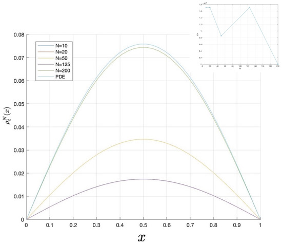
The result of Theorem 4 is depicted in Figure 6, where the error in terms of $L^2-$norm is also provided.

Figure 6. Plot of sample trajectories of ${\rho }_t^N\left(x\right)$, solution of equation (61), for $x\in$ with $D=[0,1]$, $t=1$ and different values of N. In blue the trajectory of the solution of the deterministic PDE (66)–(68). In the corner on the right a plot of the error in terms of the $L^2-$norm.

By the linear stability of problem (66)–(68), since the diffusion coefficient is small (see [26]), we again obtain that ${\rho }_c=1-2\frac{r_d}{r_b}$ is stable whilst the trivial steady-state ${\rho }_{nc}=0$ is unstable. Therefore, the diffusion has no effect on the stability of the spatial homogeneous steady-sates and again the cancerous population survives.

7. Discussion

In the current paper, we have introduced a novel averageaveraging method to deal with the study of the dynamics of a class of RODEs and RPDEs since classical averaging methods fail to treat this kind of problem. To elucidate the relevance of our theoretical results, we apply this method to an important biomedical problem, i.e., the assessment of intratumoral heterogeneity impact on tumor dynamics. In particular, we consider the development of gliomas according to a well-known Go or Grow (GoG) model, where intratumoral heterogeneity is modeled as a stochastic process. It has been shown that the deterministic version of the considered GoG model exhibits an emerging Allee effect (bistability). On the other hand, for the novel stochastic version of the GoG model, we demonstrate that the introduction of white noise, as a model of intratumoral heterogeneity, leads to monostable tumor growth. The latter entails the disappearance of the Allee effect, and thus we conclude that the extinction is impossible under parametric variations. Consequently, our results suggest that the existence of heterogeneity worsens the prognosis of tumor growth, which is actually in accordance with the clinical experience and literature [27,28].

The GoG mechanism has been firstly identified in gliobslastoma tumours by Giese and his colleagues [29]. However, the migration/proliferation plasticity has been found to be relevant in other tumors, such as breast cancer [30], melanoma [31], and more. Additionally, a dichotomy between cell proliferation and invasive behavior has been identified in normal tissue development [32]. As we have shown already this switching mechanism between proliferative and migrative phases can induce a heterogeneity in the invasive behavior of a cell collective and eventually impact the corresponding collective dynamics. Our proposed methodology could be helpful in analyzing data from these different biological systems.

The assumption of white noise is the worst possible scenario related to tumor heterogeneity, and therefore other noise distributions should be analyzed such as Gaussian noise. This case is going to be investigated in a forthcoming paper. Moreover, there have been a plethora of studies trying to quantify intratumoral heterogeneity, see [33,34,35,36], nevertheless our method is able to include the existing literature and analyze the impact of data-driven heterogeneity distribution in more realistic tumor models. For instance, data regarding the invasive behavior heterogeneity, e.g., migration speed distribution, of tumor cells can be easily integrated and analyzed from our framework, such as in [37]. Furthermore, our method can be also implemented to investigate the long-time dynamics of the full GoG system (52) and (53), which will be the subject of a forthcoming work.

References

- Freidlin, M.I.; Wentzell, A.D. Random perturbations. In Random Perturbations of Dynamical Systems; Springer: Berlin/Heidelberg, Germany, 1998; pp. 15–43. [Google Scholar]
- Bogoliubov, N.N.; Mitropolskij, J.A.; Mitropolskii, I.A.; Mitropolsky, Y.A. Asymptotic Methods in the Theory of Non-Linear Oscillations; CRC Press: Boca Raton, FL, USA, 1961; Volume 10. [Google Scholar]
- Volosov, V.M. Averaging in systems of ordinary differential equations. Russ. Math. Surv. 1962, 17, 1–126. [Google Scholar] [CrossRef]
- Sanders, J.A.; Verhulst, F.; Murdock, J. Averaging Methods in Nonlinear Dynamical Systems; Springer: Berlin/Heidelberg, Germany, 2007; Volume 59. [Google Scholar]
- Pavliotis, G.; Stuart, A. Multiscale Methods: Averaging and Homogenization; Springer: New York, NY, USA, 2008. [Google Scholar]
- Han, X.; Kloeden, P.E. Random Ordinary Differential Equations and Their Numerical Solution; Probability Theory and Stochastic Modelling 85; Springer: Berlin/Heidelberg, Germany, 2017. [Google Scholar]
- Meacham, C.E.; Morrison, S.J. Tumour heterogeneity and cancer cell plasticity. Nature 2013, 501, 328–337. [Google Scholar] [CrossRef] [PubMed]
- McGranahan, N.; Swanton, C. Biological and therapeutic impact of intratumor heterogeneity in cancer evolution. Cancer Cell 2015, 27, 15–26. [Google Scholar] [CrossRef] [PubMed]
- Hatzikirou, H.; Basanta, D.; Simon, M.; Schaller, K.; Deutsch, A. Go or Grow: The key to the emergence of invasion in tumour progression? Math. Med. Biol. J. IMA 2012, 29, 49–65. [Google Scholar] [CrossRef] [PubMed]
- Goodenberger, M.L.; Jenkins, R.B. Genetics of adult glioma. Cancer Genet. 2012, 205, 613–621. [Google Scholar] [CrossRef] [PubMed]
- Sanai, N.; Alvarez-Buylla, A.; Berger, M.S. Neural stem cells and the origin of gliomas. N. Engl. J. Med. 2005, 353, 811–822. [Google Scholar] [CrossRef] [PubMed]
- Tektonidis, M.; Hatzikirou, H.; Chauvière, A.; Simon, M.; Schaller, K.; Deutsch, A. Identification of intrinsic in vitro cellular mechanisms for glioma invasion. J. Theor. Biol. 2011, 287, 131–147. [Google Scholar] [CrossRef] [PubMed]
- Böttger, K.; Hatzikirou, H.; Voss-Bxoxhme, A.; Cavalcanti-Adam, E.A.; Herrero, M.A.; Deutsch, A. An Emerging Allee Effect Is Critical for Tumor Initiation and Persistence. PLoS Comput. Biol. 2015, 11, e1004366. [Google Scholar] [CrossRef]
- Alfonso, J.C.L.; Talkenberger, K.; Seifert, M.; Klink, B.; Hawkins-Daarud, A.; Swanson, K.R.; Hatzikirou, H.; Deutsch, A. The biology and mathematical modelling of glioma invasion: A review. J. R. Soc. Interface 2017, 14, 1–20. [Google Scholar] [CrossRef]
- Alfonso, J.C.L.; Köhn-Luque, A.; Stylianopoulos, T.; Feuerhake, F.; Deutsch, A.; Hatzikirou, H. Why one-size-fits-all vaso-modulatory interventions fail to control glioma invasion: In silico insights. Sci. Rep. 2016, 6, 37283. [Google Scholar] [CrossRef]
- Hatzikirou, H.; Alfonso, J.C.L.; Mühle, S.; Stern, C.; Weiss, S.; Meyer-Hermann, M. Cancer therapeutic potential of combinatorial immuno- and vaso-modulatory interventions. J. R. Soc. Interface 2015, 12, 20150439. [Google Scholar] [CrossRef]
- Mascheroni, P.; Alfonso, J.C.L.; Kalli, M.; Stylianopoulos, T.; Meyer-Hermann, M.; Hatzikirou, H. On the impact of chemo-mechanically induced phenotypic transitions in gliomas. Cancers 2019, 11, 716. [Google Scholar] [CrossRef]
- Gelfand, I.M.; Shilov, G.E. Generalized Functions, Vol. 4: Applications of Harmonic Analysis; Academic Press: Cambridge, MA, USA, 1964. [Google Scholar]
- Hsu, S.-B. Ordinary Differential Equations with Applications, 2nd ed.; World Scientific: Singapore, 2013. [Google Scholar]
- Ladyženskaja, O.; Solonnikov, V.A.; Ural’ceva, N.N. Linear and Quasi-Linear Equations of Parabolic Type; American Mathematical Society: Providence, RI, USA, 1968. [Google Scholar]
- Stein, E. Harmonic Analysis: Real-Variable Methods, Orthogonality, and Oscillatory Integrals; Princeton University Press: Princeton, NJ, USA, 1993. [Google Scholar]
- Stein, E.M.; Shakarchi, R. Real Analysis, 1st ed.; Princeton Lectures in Analysis, 3; Princeton University Press: Princeton, NJ, USA, 2005. [Google Scholar]
- Henry, D. Geometric Theory of Semilinear Parabolic Equations; Lecture Notes in Mathematics; Springer: Berlin/Heidelberg, Germany, 2006. [Google Scholar]
- Duan, J.; Wang, W. Effective Dynamics of Stochastic Partial Differential Equations; Elsevier: Amsterdam, The Netherlands, 2014. [Google Scholar]
- Hatzikirou, H.; Boettger, K.; Deutsch, A. Model-based Comparison of Cell Density-dependent Cell Migration Strategies. Math. Model. Nat. Phenom. 2015, 10, 94–107. [Google Scholar] [CrossRef][Green Version]
- Murray, J. Mathematical Biology Vol II: Spatial Models and Biomedical Applications; Springer: Berlin/Heidelberg, Germany, 2003. [Google Scholar]
- Dagogo-Jack, I.; Shaw, A.T. Tumour heterogeneity and resistance to cancer therapies. Nat. Rev. Clin. Oncol. 2018, 15, 81–94. [Google Scholar] [CrossRef]
- Ramón y Cajal, S.; Sesé, M.; Capdevila, C.; Aasen, T.; De Mattos-Arruda, L.; Diaz-Cano, S.J.; Castellví, J. Clinical implications of intratumor heterogeneity: Challenges and opportunities. J. Mol. Med. 2020, 98, 161–177. [Google Scholar] [CrossRef]
- Giese, A.; Loo, M.; Tran, N.; Haskett, S.W.; Berens, M.E. Dichotomy of astrocytoma migration and proliferation. Int. J. Cancer 1996, 67, 275–282. [Google Scholar] [CrossRef]
- Jerby, L.; Wolf, L.; Denkert, C.; Stein, G.Y.; Hilvo, M.; Oresic, M.; Ruppin, E. Metabolic associations of reduced proliferation and oxidative stress in advanced breast cancer. Cancer Res. 2012, 72, 5712–5720. [Google Scholar] [CrossRef]
- Kemper, K.; De Goeje, P.L.; Peeper, D.S.; Van Amerongen, R. Phenotype switching: Tumor cell plasticity as a resistance mechanism and target for therapy. Cancer Res. 2014, 74, 5937–5941. [Google Scholar] [CrossRef]
- Kohrman, A.Q.; Matus, D.Q. Divide or Conquer: Cell Cycle Regulation of Invasive Behavior. Trends Cell Biol. 2017, 27, 12–25. [Google Scholar] [CrossRef]
- Alic, L.; Niessen, W.J.; Veenland, J.F. Quantification of heterogeneity as a biomarker in tumor imaging: A systematic review. PLoS ONE 2014, 9, e110300. [Google Scholar] [CrossRef]
- Oesper, L.; Satas, G.; Raphael, B.J. Quantifying tumor heterogeneity in whole-genome and whole-exome sequencing data. Bioinformatics 2014, 30, 3532–3540. [Google Scholar] [CrossRef] [PubMed]
- Rutter, E.M.; Banks, H.T.; Flores, K.B. Estimating intratumoral heterogeneity from spatiotemporal data. J. Math. Biol. 2018, 77, 1999–2022. [Google Scholar] [CrossRef] [PubMed]
- Sottoriva, A.; Spiteri, I.; Piccirillo, S.G.M.; Touloumis, A.; Collins, V.P.; Marioni, J.C.; Curtis, C.; Watts, C.; Tavaré, S. Intratumor heterogeneity in human glioblastoma reflects cancer evolutionary dynamics. Proc. Natl. Acad. Sci. USA 2013, 110, 4009–4014. [Google Scholar] [CrossRef] [PubMed]
- Parker, J.J.; Canoll, P.; Niswander, L.; Kleinschmidt-DeMasters, B.K.; Foshay, K.; Waziri, A. Intratumoral heterogeneity of endogenous tumor cell invasive behavior in human glioblastoma. Sci. Rep. 2018, 8, 1–10. [Google Scholar] [CrossRef]
Publisher’s Note: MDPI stays neutral with regard to jurisdictional claims in published maps and institutional affiliations. |
© 2021 by the authors. Licensee MDPI, Basel, Switzerland. This article is an open access article distributed under the terms and conditions of the Creative Commons Attribution (CC BY) license (https://creativecommons.org/licenses/by/4.0/).