On Triangle-Free v₃ Configurations

Abstract

We describe a classification algorithm of combinatorial triangle-free $v_3$-configurations. The (non-isomorphic) triangle-free $v_3$ configurations are classified for $v\in \{23,24\}$. We conclude that there is no triangle-free $v_3$ configuration that is blocking set free for $v\le 24$. We also give some statistics on some properties of the structures, like transitivity, self-duality, and self-polarity.

1. Introduction

An incidence structure $\mathcal{X}$ is a pair $(\mathcal{P},\mathcal{B})$, where $\mathcal{P}$ is a set of v points$\{p_1,\cdots ,p_v\}$ and $\mathcal{B}$ is a collection of b blocks (also called lines) $\{B_1,B_2,\cdots ,B_b\}$ such that $B_i\subseteq \mathcal{P}$ for $i=1,\cdots ,b$. We write $\left[p\right]$ to denote the number of blocks containing p and $\left|B\right|$ to denote the number of points contained in B. A flag is a pair $(p,B)$ with $p\in B\in \mathcal{B}.$ In this case, we say that p and B are incident. An anti-flag is a pair $(p,B)$ with $p\notin B\in \mathcal{B}.$

A (combinatorial) configuration of type $(v_r,b_k)$ is an incidence structure $(\mathcal{P},\mathcal{B})$ satisfying the following three conditions:

(I) 

Each point is contained in r blocks; $\left[p_i\right]=r$ for $i=1,\cdots ,v$.

(II) 

Each block (line) contains k points; $|B_j| =k$ for $j=1,\cdots ,b$.

(III) 

Any pair of distinct points is contained in at most one block; $|B_i\cap B_j| \le 1$ for $i,j\in \{1,\cdots ,b\}$, $i\ne j$.

In a configuration $(v_r,b_k)$, the parameters are related by means of the fundamental equation $vr=kb,$ which follows by counting flags in two ways. A $(v_r,b_k)$ configuration is called symmetric if $v=b$ (and hence $r=k$). In that case, it is denoted simply by $v_k$. A configuration is trivial if $k=2$ or $k=v.$ We do not care very much about these two examples, hence we will assume that our configurations are non-trivial.

Two configurations ${\mathcal{C}}_1=({\mathcal{P}}_1,{\mathcal{B}}_1)$ and ${\mathcal{C}}_2=({\mathcal{P}}_2,{\mathcal{B}}_2)$ are said to be isomorphic if there is a mapping $\alpha$: ${\mathcal{P}}_1\to {\mathcal{P}}_2$ that takes ${\mathcal{B}}_1$ to ${\mathcal{B}}_2$. An isomorphism from a configuration $\mathcal{C}$ to itself is called an automorphism. The concatenation of two automorphisms is another automorphism, as is the inverse of an automorphism. For this reason, the set of automorphisms forms a group, the automorphism group of the incidence structure. The automorphism group of a configuration $\mathcal{C}$ is denoted by $\mathrm{Aut}\left(\mathcal{C}\right)$.

A triangle (or 3-cycle) in a configuration $\mathcal{C}$ is a triple of points that are pairwise collinear but not with the same line. A triangle-free $v_3$ configuration, abbreviated TFC $v_3$, is a $v_3$ configuration with no triangles. For later reference, we pose the condition explicitly as follows:

(IV) 

There are no three points pairwise collinear but not in a line.

Triangle-free configurations are of considerable interest. In the theory of geometric incidence structures (with no more than one block per each pair of points), the process of tactical refinement leads to tactical decompositions, which consist of an array of configurations. In this sense, one could call tactical configurations the “atomic objects” in the world of geometric incidence geometries: They are the objects that make up larger incidence structures. The property of triangle-freeness helps to single out the most interesting objects in the vast class of configurations.

One further application of triangle-free configurations exists: The well-studied class of objects called generalized quadrangles are triangle-free configurations with an extra condition:

(V) 

If a point P is not incident with a line ℓ, then there is a unique point Q on ℓ collinear with P.

For the sake of completeness, a generalized quadrangle $\mathrm{GQ}(s,t)$ is a $(v_r,b_k)$ configuration with

$$v=(st+1)(s+1), b=(st+1)(t+1), r=t+1,k=s+1,$$

(1)

satisfying condition (V). To be clear, this paper is not a contribution to the study of generalized quadrangles. Therefore, in what follows we will not explicitly ask for condition (V). The study of triangle-free configurations is broader than the study of generalized quadrangles. However, it may be the case that condition (V) is satisfied accidentally.

Generalized quadrangles were first introduced by Tits in [1]. For more on the theory of generalized quadrangles, see [2]. For a beautiful treatment of the relationships between designs, codes, graphs and geometries, including generalized quadrangles; see [3].

The incidence matrix of a configuration is defined provided an ordering of points and blocks has been chosen. The incidence matrix has rows corresponding to the points and columns corresponding to the blocks. An entry in a row and a column is one if the associated pair of point and line are incident (i.e., form a flag). Thus, the incidence matrix completely determines the geometry and conversely. Therefore, the study of configurations can be seen as the study of certain matrices with entries in $\{0,1\}.$ Properties of the geometry translate into properties of the incidence matrix. For instance, the number of ones in any row is equal to r. Likewise, the number of ones in any column is equal to k. Moreover, because two points determine at most one block, there is no

$$\left[\begin{array}{cc}1& 1\\ 1& 1\end{array}\right]$$

submatrix anywhere in the matrix. For a triangle-free incidence structure, we must exclude any submatrix that looks like this,

$$\left[\begin{array}{ccc}1& 1& 0\\ 1& 0& 1\\ 0& 1& 1\end{array}\right]$$

(2)

disregarding the ordering of rows and columns.

2. Outline of the Paper

The outline of this paper is this: In Section 3, we will look at the smallest example of the kind of object we wish to study. It has been studied before, and it shows the tight connection between finite geometry and combinatorics. In Section 4, we state our main results. In Section 5 we discuss further notions regarding the action of the automorphism group. We also explore the important connection between incidence structures and a class of bipartite graphs. In Section 6, we look at the embeddability of the configuration in the real plane. In Section 7, we discuss the important problem of classification for finite incidence structures. In Section 8 we describe our search algorithm and give details about the computation for the cases $v=23$ and $v=24$. In Section 9, we will take a closer look at some of the more interesting examples of configurations that we found, revisiting the questions that we discussed earlier, like embeddability in the real plane and properties of the automorphism group. Finally, in Section 10, we draw some conclusions from our work.

3. The Smallest Example

The smallest configuration $v_3$ is the Fano plane $7_3$. It is the incidence relation of the projective plane over the field with two elements. This configuration has many triangles.

The smallest triangle-free configuration $v_3$ is the Cremona–Richmond configuration ${15}_3.$ It is in fact a generalized quadrangle, namely a $\mathrm{GQ}(2,2).$ It arises in the theory of cubic surfaces from the incidence between lines and tritangent planes of the cubic surface in projective three-space given by the equation

$$X_0^2{X}_3+X_1^2{X}_2+X_1{X}_2^2+X_0{X}_3^2=0$$

(3)

in the field ${\mathbb{F}}_2$ (see Karaoglu [4]). Namely, the configuration is the incidence geometry between the 15 lines of the surface and the 15 tritangent planes. The automorphism group of the Cremona–Richmond configuration coincides with the automorphism group of the cubic surface over the field ${\mathbb{F}}_2$. It is isomorphic to $\mathrm{Sym}\left(6\right)$, the symmetric group on 6 letters, of order 720.

For a better understanding of the geometry, it is helpful to extend the field of definition to a field ${\mathbb{F}}_4$. Over this field, the surface has 27 lines, and it contains the geometry with 15 lines as a subfield subgeometry. In Schläfli labels (see [5]), we may take the lines to be the

$$c_{ij},1\le i<j\le 6,$$

and the planes to be the tritangent planes with labels

$${\pi }_{ij,kl,mn}$$

where $i,j,k,l,m,n$ are permutations of the six letters 1 through 6. For a detailed list of the lines and planes (in the subfield subgeometry), see below. At first, we list the 15 lines. Following a convention from coding theory, we display a $2\times 4$ matrix whose rowspan is the subspace whose projectivization is the line; see Table 1.

Table 1. The points in the Cremona–Richmond configurations are the lines of a cubic surface over the field ${\mathbb{F}}_2$.

$$c_{12}=\left[\begin{array}{cccc}\hfill 1& 0& 1& 0\\ \hfill 0& 1& 1& 1\end{array}\right]$$	$$c_{13}=\left[\begin{array}{cccc}\hfill 0& 0& 1& 0\\ \hfill 0& 0& 0& 1\end{array}\right]$$	$$c_{14}=\left[\begin{array}{cccc}\hfill 1& 0& 0& 1\\ \hfill 0& 1& 1& 0\end{array}\right]$$
$$c_{15}=\left[\begin{array}{cccc}\hfill 1& 0& 1& 1\\ \hfill 0& 1& 0& 1\end{array}\right]$$	$$c_{16}=\left[\begin{array}{cccc}\hfill 1& 0& 0& 0\\ \hfill 0& 1& 0& 0\end{array}\right]$$	$$c_{23}=\left[\begin{array}{cccc}\hfill 1& 0& 0& 0\\ \hfill 0& 1& 1& 0\end{array}\right]$$
$$c_{24}=\left[\begin{array}{cccc}\hfill 0& 1& 0& 0\\ \hfill 0& 0& 0& 1\end{array}\right]$$	$$c_{25}=\left[\begin{array}{cccc}\hfill 1& 1& 0& 0\\ \hfill 0& 0& 1& 1\end{array}\right]$$	$$c_{26}=\left[\begin{array}{cccc}\hfill 1& 0& 0& 1\\ \hfill 0& 0& 1& 0\end{array}\right]$$
$$c_{34}=\left[\begin{array}{cccc}\hfill 1& 0& 1& 1\\ \hfill 0& 1& 1& 1\end{array}\right]$$	$$c_{35}=\left[\begin{array}{cccc}\hfill 1& 0& 0& 1\\ \hfill 0& 1& 0& 0\end{array}\right]$$	$$c_{36}=\left[\begin{array}{cccc}\hfill 1& 0& 1& 0\\ \hfill 0& 1& 0& 1\end{array}\right]$$
$$c_{45}=\left[\begin{array}{cccc}\hfill 1& 0& 0& 0\\ \hfill 0& 0& 1& 0\end{array}\right]$$	$$c_{46}=\left[\begin{array}{cccc}\hfill 1& 1& 0& 1\\ \hfill 0& 0& 1& 1\end{array}\right]$$	$$c_{56}=\left[\begin{array}{cccc}\hfill 0& 1& 1& 0\\ \hfill 0& 0& 0& 1\end{array}\right]$$

Next, we display the 15 subspaces that are the planes. Note that $\mathrm{PG}(3,2)$ has 15 planes, so all planes arise in this setting. However, in $\mathrm{PG}(3,4)$ only 45 tritangent planes arise, and only 15 belong to the subfield subgeometry. Here, $\mathbf{v}$ stands for variety and $X_0,X_1,X_2,X_3$ are the coordinate functionals of ${\mathbb{F}}^4,$ i.e., the homogeneous coordinates of $\mathrm{PG}(3,\mathbb{F}).$ For a list of the planes, see Table 2.

Table 2. The lines in the Cremona–Richmond configuration are the tritangent planes of a cubic surface over the field ${\mathbb{F}}_2$.

$$\begin{array}{ccc}\hfill {\mathit{\pi }}_{12,34,56}& =& \mathbf{v}\left(X_0+X_1+X_2\right)\hfill \\ \hfill {\mathit{\pi }}_{12,35,46}& =& \mathbf{v}\left(X_0+X_2+X_3\right)\hfill \\ \hfill {\mathit{\pi }}_{12,36,45}& =& \mathbf{v}\left(X_1+X_3\right)\hfill \\ \hfill {\mathit{\pi }}_{13,24,56}& =& \mathbf{v}\left(X_0\right)\hfill \\ \hfill {\mathit{\pi }}_{13,25,46}& =& \mathbf{v}\left(X_0+X_1\right)\hfill \\ \hfill {\mathit{\pi }}_{13,26,45}& =& \mathbf{v}\left(X_1\right)\hfill \\ \hfill {\mathit{\pi }}_{14,23,56}& =& \mathbf{v}\left(X_1+X_2\right)\hfill \\ \hfill {\mathit{\pi }}_{14,25,36}& =& \mathbf{v}\left(X_0+X_1+X_2+X_3\right)\hfill \\ \hfill {\mathit{\pi }}_{14,26,35}& =& \mathbf{v}\left(X_0+X_3\right)\hfill \\ \hfill {\mathit{\pi }}_{15,23,46}& =& \mathbf{v}\left(X_1+X_2+X_3\right)\hfill \\ \hfill {\mathit{\pi }}_{15,24,36}& =& \mathbf{v}\left(X_0+X_2\right)\hfill \\ \hfill {\mathit{\pi }}_{15,26,34}& =& \mathbf{v}\left(X_0+X_1+X_3\right)\hfill \\ \hfill {\mathit{\pi }}_{16,23,45}& =& \mathbf{v}\left(X_3\right)\hfill \\ \hfill {\mathit{\pi }}_{16,24,35}& =& \mathbf{v}\left(X_2\right)\hfill \\ \hfill {\mathit{\pi }}_{16,25,34}& =& \mathbf{v}\left(X_2+X_3\right)\hfill \end{array}$$

The incidence in the Cremona–Richmond configuration is natural, i.e., inclusion of subspaces in the underlying vector space. In terms of the Schläfli labels (see [5]), the incidence can be described by the well-known rules. Namely, $c_{ij}\in {\pi }_{ab,cd,ef}$ if and only if $\{i,j\}=\{a,b\}$ or $\{i,j\}=\{c,d\}$ or $\{i,j\}=\{e,f\}.$

One word about the automorphism group. Over the field ${\mathbb{F}}_2$, the cubic surface has an automorphism group of order 720, and this is also the automorphism group of the Cremona–Richmond configuration. The group has a natural representation on $\mathrm{GL}(4,2)$ as invertible $4\times 4$ matrices over the field with two elements. If the equation is considered over the field with 4 elements, the surface has 27 lines and the group becomes larger. In fact, the projective group is the Weyl group of type $E_6$, of order $25920.$ It is a simple group, see [6]. It has a subfield subgroup which is isomorphic to the group of order 720 which stabilizes the cubic surface over ${\mathbb{F}}_2.$

Some historical comments are in order. Equation (3) was mentioned in the work of Dickson [7], where the geometry of the 15 lines was mentioned. The Cremona–Richmond configuration is named after Cremona [8] and Richmond [9], but it was also discussed by Martinetti [10].

The incidence matrix of the Cremona–Richmond configuration is shown in Table 3. As one can check, it satisfies all the requirements.

Table 3. The incidence matrix of the Cremona–Richmond configuration.

$$\left[\begin{array}{cccccccccccccccc}12& 1& 1& 1& 0& 0& 0& 0& 0& 0& 0& 0& 0& 0& 0& 0\\ 13& 0& 0& 0& 1& 1& 1& 0& 0& 0& 0& 0& 0& 0& 0& 0\\ 14& 0& 0& 0& 0& 0& 0& 1& 1& 1& 0& 0& 0& 0& 0& 0\\ 15& 0& 0& 0& 0& 0& 0& 0& 0& 0& 1& 1& 1& 0& 0& 0\\ 16& 0& 0& 0& 0& 0& 0& 0& 0& 0& 0& 0& 0& 1& 1& 1\\ 23& 0& 0& 0& 0& 0& 0& 1& 0& 0& 1& 0& 0& 1& 0& 0\\ 24& 0& 0& 0& 1& 0& 0& 0& 0& 0& 0& 1& 0& 0& 1& 0\\ 25& 0& 0& 0& 0& 1& 0& 0& 1& 0& 0& 0& 0& 0& 0& 1\\ 26& 0& 0& 0& 0& 0& 1& 0& 0& 1& 0& 0& 1& 0& 0& 0\\ 34& 1& 0& 0& 0& 0& 0& 0& 0& 0& 0& 0& 1& 0& 0& 1\\ 35& 0& 1& 0& 0& 0& 0& 0& 0& 1& 0& 0& 0& 0& 1& 0\\ 36& 0& 0& 1& 0& 0& 0& 0& 1& 0& 0& 1& 0& 0& 0& 0\\ 45& 0& 0& 1& 0& 0& 1& 0& 0& 0& 0& 0& 0& 1& 0& 0\\ 46& 0& 1& 0& 0& 1& 0& 0& 0& 0& 1& 0& 0& 0& 0& 0\\ 56& 1& 0& 0& 1& 0& 0& 1& 0& 0& 0& 0& 0& 0& 0& 0\end{array}\right]$$

For an embedding in the real plane, see Figure 1 (picture credit: David Eppstein, Wikipedia). More about real embeddings will be said in Section 6.

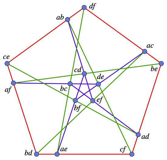
Figure 1. The Cremona Richmond Configuration.

The automorphism group of the Cremona–Richmond configuration is isomorphic to the group $\mathrm{Sym}\left(6\right)$ of order 720. In the model that we just described, the generators are $4\times 4$ matrices over the field ${\mathbb{F}}_2,$ see Table 4.

Table 4. Coxeter generators for the automorphism group of the Cremona–Richmond configuration.

$$\begin{array}{ccc}\hfill s_1& =& \left[\begin{array}{cccc}\hfill 0& 1& 1& 1\\ \hfill 1& 0& 1& 1\\ \hfill 1& 1& 0& 1\\ \hfill 1& 1& 1& 0\end{array}\right],s_2=\left[\begin{array}{cccc}\hfill 1& 1& 1& 1\\ \hfill 0& 0& 1& 1\\ \hfill 0& 1& 0& 1\\ \hfill 0& 0& 0& 1\end{array}\right],s_3=\left[\begin{array}{cccc}\hfill 1& 0& 1& 1\\ \hfill 0& 1& 1& 1\\ \hfill 0& 0& 1& 0\\ \hfill 0& 0& 0& 1\end{array}\right],\hfill \\ \hfill s_4& =& \left[\begin{array}{cccc}\hfill 1& 0& 0& 0\\ \hfill 1& 1& 1& 0\\ \hfill 0& 0& 1& 0\\ \hfill 1& 0& 1& 1\end{array}\right],s_5=\left[\begin{array}{cccc}\hfill 1& 0& 0& 0\\ \hfill 0& 1& 0& 0\\ \hfill 1& 1& 1& 0\\ \hfill 1& 1& 0& 1\end{array}\right].\hfill \end{array}$$

The chosen generators are Coxeter generators associated with the root system of type $A_5$. This means that

$$\begin{array}{ccc}\hfill s_i^2& =& \mathrm{id},\hspace{1em}i=1,\dots ,5\hfill \\ \hfill {\left(s_i{s}_{i+1}\right)}^3& =& \mathrm{id},\hspace{1em}i=1,\dots ,4\hfill \\ \hfill {\left(s_i{s}_j\right)}^2& =& \mathrm{id},\hspace{1em}i=1,\dots ,5, j=1,\dots ,5, |i-j|\ge 2\hfill \end{array}$$

The action of the automorphism group is as follows: The image of the point (which is a line) given by the generator matrix B under the group element G is the line with generator matrix $BG.$ The image of the line (which is a hyperplane) written as $\mathrm{v}(a_0{x}_0+a_1{x}_1+a_2{x}_2+a_3{x}_3)$ is given by linear substitution of the columns of $G^{-1}$ where G is the matrix of the automorphism.

4. Main Results

Triangle freeness is a very restrictive and therefore interesting property. For instance, it is known that there are exactly 245,342 configurations of ${15}_3$, up to isomorphism (see [11]). However, only one of these is triangle-free. The number of isomorphism types of configurations $v_3$ grows very quickly with v.

Considering the fact that there are so many configurations and only very few are triangle-free, we wish to draw attention to the few triangle-free ones. This leads to our main question: Are there other triangle-free configurations $v_3$? And, as a follow-up, we may ask: If so, do they have nice descriptions as geometric objects (like the Cremona–Richmond ${15}_3$)?

In [11,12], triangle-free $v_3$ configurations are classified for $v\le 21$. Later, in [13], the case $v=22$ was settled. Here, we continue the classification for $v=23$ and $v=24.$ Our results are summarized in Table 5. We list the number of triangle-free $v_3$ configurations for $15\le v\le 24,$ including the number of those with special properties, like self-dual and self-polar. We also list special properties like point transitive ones, flag transitive ones, and those without a blocking set. For $v<15,$ there are no triangle-free configurations $v_3.$ More detailed results about the objects will follow in Section 9.

Table 5. Triangle-free $v_3$ configurations for $15\le v\le 24$. Note: A is the number of configurations of $v_3$, B is the number of self-dual configurations of $v_3$, C is the number of self-polar configurations of $v_3$, D is the number of point-transitive configurations of $v_3$, E is the number of flag-transitive configurations of $v_3$, and F is the number of blocking-set-free configurations of $v_3$.

${\mathit{v}}_3$	A	B	C	D	E	F
15	1	1	1	1	1	0
16	0	0	0	0	0	0
17	1	1	1	0	0	0
18	4	2	2	0	0	0
19	14	6	6	0	0	0
20	162	40	40	1	1	0
21	4713	307	303	1	0	0
22	157,211	1999	1992	0	0	0
23	5,202,095	13,095	13,082	0	0	0
24	163,348,199	84,633	84,593	3	1	0

Our main tool to classify triangle-free $v_3$ configurations for small values of v is based on that search. We will also investigate the properties of the configurations found. Among the triangle-free configurations, we are particularly interested in those which have a large automorphism group.

For further background material on configurations, see [14]. For a recent contribution to the study of combinatorial configurations embedded in finite geometries, see [15]. An early study of cubic surfaces and associated configurations is [16]. For recent applications to quantum computing, see [17].

5. Further Comments

Much information can be gained about the structure of a configuration by studying the automorphism group and its action on the object and the associated objects. Examples of associated objects are the set of points, the set of lines, the set of flags, and the set of anti-flags. For starters, here is some commonly used terminology: If a group G acts transitively on a class of objects $\mathfrak{O}$, we say that G is $\mathfrak{O}$-transitive. An orbit on objects of type $\mathfrak{O}$ is called an $\mathfrak{O}$-orbit.

The orbit type of a configuration $\mathcal{C}$ is the pair $(h_1,h_2)$ where $h_1$ is the number of point-orbits and $h_2$ is the number of block-orbits of the automorphism group. It is simply called of orbit type h if it has $h=h_1=h_2$.

It is interesting to study various transitivity properties of automorphism groups of incidence structures. It is well-known that a flag-transitive automorphism group G is also transitive on points and blocks, but not conversely. For more background on incidence geometries and their groups, see Dembowski [18]. In a design, transitivity on blocks implies transitivity on points, see [19]. For a recent contribution to flag-transitive large sets of configurations; see [20].

Yet another concept is that of a blocking set. The blocking set in a configuration $\mathcal{C}$ is a subset Q of points such that each block contains at least one element in Q and one element not in Q. A blocking-set-free configuration is a configuration that contains no blocking sets.

Configurations are closely related to graphs. Given a configuration $\mathcal{C}$, the Levi graph of $\mathcal{C}$, denoted by $L\left(\mathcal{C}\right)$, is the bipartite graph with a black vertex for each point, a white vertex for each block, and an edge connecting two vertices of different colors if and only if the corresponding point and block are incident in $\mathcal{C}$. The correspondence with Levi graphs is functorial. Namely, isomorphisms between configurations correspond to isomorphisms of the associated Levi graphs. This is because the action of the symmetric group on incidence structures (with action on points and blocks) corresponds to the action of the symmetric group on the Levi graphs, stabilizing the partition of the vertices. The action on flags of the incidence structure is the same as the action on edges in the Levi graph. Therefore, Levi graphs are isomorphic precisely if the corresponding incidence structures are. In addition, the automorphism group of an incidence structure and the automorphism group of the associated Levi graph are isomorphic.

It is well-known that an incidence structure $\mathcal{C}$ is a $v_3$-configuration if and only if its Levi graph is cubic and has girth (the length of the shortest cycle) at least 6.

Proposition 1 (Coxeter [21]). 

An incidence structure C is a $v_3$ configuration if and only if its Levi graph is cubic and has girth at least 6.

To be precise, a cycle of length $2g$ in the Levi graph $L\left(\mathcal{C}\right)$ corresponds to a g-gon in the configuration $\mathcal{C}$. In particular, a hexagon in $L\left(\mathcal{C}\right)$ corresponds to a triangle in $\mathcal{C}$. Therefore, $\mathcal{C}$ is TFC if and only if its Levi graph has girth at least 8.

The dual configuration ${\mathcal{C}}^{\ast }=(\mathcal{B},\mathcal{P})$ of a $v_3$ configuration $\mathcal{C}=(\mathcal{P},\mathcal{B})$ is defined by reversing the roles of points and blocks in $\mathcal{C}$, but with the same incidences. Consequently, the Levi graphs of $\mathcal{C}$ and ${\mathcal{C}}^{\ast }$ are the same, except that the color classes are reversed. A configuration $\mathcal{C}$ is said to be self-dual if it is isomorphic to its dual ${\mathcal{C}}^{\ast }$. The corresponding isomorphism then is called duality. A duality of order 2 is called a polarity. A configuration $\mathcal{C}$ is called self-polar if it admits a polarity. Dualities and polarities are important because they allow us to see more symmetry than what can be detected with isomorphisms alone. For instance, a projective space always has a polarity that reverses the inclusion of subspaces. The reason is that the underlying lattice of subspaces has an anti-automorphism. The anti-automorphism turns the order structure “upside-down”. So, the question of whether a polarity exists is asking if the incidence structure has an incidence-reversing mapping, similar to the anti-automorphism in the case of a projective geometry. Of course, for a polarity to exist, the configuration must be symmetric, i.e., the number of points must equal the number of lines because the two sets are put in one-to-one correspondence. The polarity group of an incidence structure is the group consisting of all polarities and isomorphisms. It contains the automorphism group as a subgroup of index at most two. For example, in Figure 2 the Fano plane is both self-dual and self-polar (through the bijection mapping $p_i\leftrightarrow B_i$ for $i=1,2,\cdots ,7$). The automorphism group of the Fano plane is the projective group $\mathrm{PGL}(3,2)$ of order 168. However, the polarity group is $\mathrm{PGL}{(3,2)}^{\ast }$ of order $336.$ Once a type of symmetric configurations has been classified by isomorphism, the polarity classes are the classes of configurations which correspond under polarity. A polarity class is either a singleton (when the configuration is self-polar) or a set of two configurations which are polar to each other.

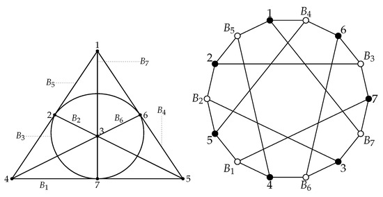
Figure 2. The Fano plane and its Levi graph (Heawood graph).

In passing, we mention that the Levi graph of the Fano plane has played an important role in the early stages of the proof attempts of the four-color conjecture (now the four-color theorem). Namely, it provided the first counterexample to Kempe’s false proof of the four-color conjecture. The Fano plane is also an example of a blocking-set-free configuration.

The Levi graph of the Cremona–Richmond configuration is a graph on 30 vertices, known as Tutte’s 8-cage. It is shown in Figure 3 (picture credit: Wikipedia). The graph was explored by Tutte [22] and independently by Coxeter [23]. The automorphism group of the graph is the full automorphism group of $\mathrm{Sym}\left(6\right)$, of order 1440. A cage is a regular graph with the least number of vertices for a given girth (length of the shortest cycle). The 8-cage above is the smallest 3-regular graph with girth 8.

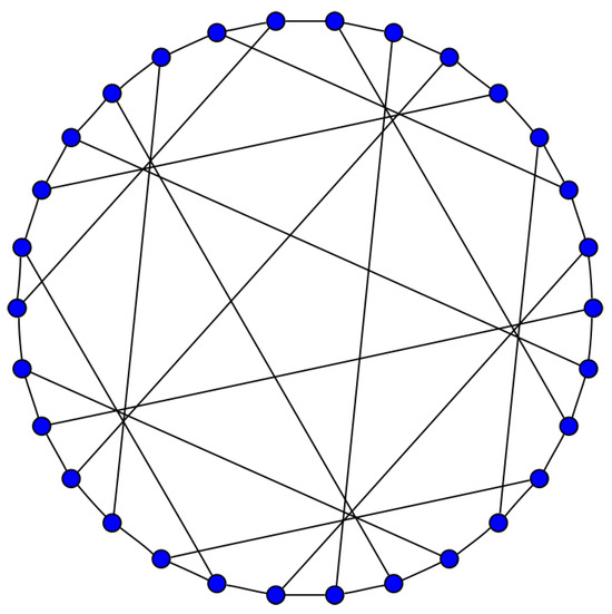
Figure 3. Tutte’s 8-Cage.

6. Embeddings in the Real Plane with Straight Lines

We note that a configuration with straight lines in the projective plane is called a geometric configuration. A configuration with pseudolines forming a rank 3 oriented matroid is called a topological configuration. A configuration with abstract lines is called a combinatorial configuration.

In this paper, we are only concerned with combinatorial configurations. For the sake of simplicity, we speak of combinatorial configurations in all of what follow unless specified otherwise.

Obviously, every geometrical (or topological) configuration is also combinatorial. However, the converse is not true and examples are known. Some methods which can be used to decide whether a given configuration can be realized geometrically and topologically can be found in [24,25,26,27,28].

7. The Classification Problem

Let G be a group acting on a set $\Omega$. The action of G on $\Omega$ defines an equivalence relation whose classes are the G-orbits on $\Omega$. For $x\in \Omega ,$ let $x^G$ denote the G-orbit of x. We collect one representative out of each G-orbit to form an orbit transversal, denoted by $\mathcal{T}$. So, an orbit transversal $\mathcal{T}$ for G on $\Omega$ is a set of elements in $\Omega$ such that for any $x\in \Omega$, there exists $g\in G$ with $x^g\in \mathcal{T}$, and for any $x,y\in \mathcal{T}$ we have $x^G\cap y^G=⌀$.

The process of constructing an orbit transversal is called classification. In our case, we will classify the triangle-free configurations for small values of v.

Definition 1. 

A canonical labeling map $\phi :\Omega \to G$ is a map satisfying the following condition for any $x,y\in \Omega$: $x\cong y$ implies $x^{\phi \left(x\right)}=y^{\phi \left(y\right)}$.

Moreover, $x^{\phi \left(x\right)}$ is called the canonical form of x and is denoted by $\rho \left(x\right)$. In particular, if $x^G=\{x,x_1,\cdots ,x_n\}$ is the G-orbit of x in $\Omega$, then $\rho \left(x\right)=\rho \left(y\right)$ for all $y\in x^G$. For that, $\rho \left(x\right)$ is also called the canonical orbit representative.

We note that the problem of classifying combinatorial objects is difficult, in general. It is very hard to estimate the complexity of the time and space for algorithms attacking such problems. Enumeration results of many interesting combinatorial objects are not known yet. Hence, classification and construction seems to be the only way to count these structures.

Several algorithms have been considered for classifying combinatorial objects. Including this paper, many algorithms have used the lexicographical order pioneered, independently, by Faradhzev [29] and Read [30]. All these algorithms rely on extensive testing and have exponential complexity.

Other algorithms use canonical forms to decide the isomorphism problem. These canonical forms are still difficult to compute. But the number of canonical form computations is much less than the number of isomorphism tests in a classification process. Most of these algorithms rely on a technique called partition backtracking. Nauty (Version 2.7r1) [31] is a software package for graph canonization developed originally by McKay, and later by McKay and Piperno [32,33].

One other technique for classifying combinatorial objects makes use of a poset structure. In that approach, a related class of “smaller” objects is classified first, and then the original objects are classified using the group invariant relation and the known classification of smaller objects. By repeating the reduction, we can utilize a poset structure of subobjects. Orbiter [34] is a software package that utilizes the concepts of poset classification.

8. Search Algorithm

A $v_3$ configuration $\mathcal{C}=(\mathcal{P},\mathcal{B})$ with $\mathcal{P}=\{p_1,p_2,\dots ,p_v\}$ and $\mathcal{B}=\{B_1,B_2,\dots ,B_v\}$ can be represented by a $\{0,1\}$-incidence matrix A with v rows (representing points) and v columns (representing lines). The $(i,j)$-entry of A is one if and only if $p_i\in B_j$ in the configuration $\mathcal{C}$. Two matrices are isomorphic if one can be obtained from the other by permuting the rows and the columns. The properties of a triangle-free $v_3$ configuration (see Section 1) are equivalent to

(I) 

each row contains three ones,

(II) 

each column contains three ones, and

(III) 

the dot product of any two (distinct) rows is at most one,

(IV) 

there is no cycle of length 3, i.e., no submatrix isomorphic to (2).

In what follows, we describe our search algorithm to classify the TFC $v_3$. The algorithm can be considered as an instance of the orderly generation method, see [35]. The algorithm can be divided into two main parts. The first one is called the generator, and the other is called the isomorph-rejector.

First, the generator carries out a row-by-row (or point-by-point) backtrack search to go over all possible incidence matrices of TFC $v_3$. It starts with the all-zero (empty) matrix. Using backtrack search, the algorithm fills the matrix one row at a time (consecutively). After filling any new row, the incidence matrix must satisfy the properties (I), (II), (III) and (IV). Here, (II) is the condition that each column contains no more than three ones. In addition, property (II) must be satisfied whenever we have completely filled the matrix.

Once a new (augmented) row is completed by the generator, the isomorph-rejector performs a test to check whether the created incidence matrix agrees with the lexicographically least form of the incidence matrix. If the answer is yes, the isomorph-rejector accepts the augmented row and proceeds with the search. Otherwise, it rejects that row and returns again to the generator for backtracking. This is how we deal with the isomorphism problem. In particular, we only accept the lexicographically least representative from each isomorphism class. Isomorphism testing is expensive, but it guarantees that we do not consider duplicated structures. Once the incidence matrix has been completed with v rows, a new TFC $v_3$ is produced.

The algorithm to create incidence geometries with v points is given next. The geometries are created in a well-defined order based on partial geometries. The algorithm comes as a pair of first/next functions. The IncGeoFirst function creates the first possible geometry if there is one. The IncGeoNext function transitions from one incidence geometry to the next or states false in case that all geometries have been constructed, see Table 6. The algorithm relies on functions RowFirstTested and RowNextTested to create the i-th row of the incidence geometry. This corresponds to filling the i-th row in the incidence matrix. The index set for rows is zero-based.

Table 6. The IncGeoFirst and IncGeoNext algorithms.

IncGeoFirst: i ← 0       while true do       while true do         if $i\ge v$ then          return true      end if                 if not RowFirstTested(i) then        break      end if      $i\leftarrow i+1$       end while       while true do         if $i=0$ then           return false         end if         $i\leftarrow i-1$                if RowNextTested(i) then           break         end if       end while       $i\leftarrow i+1$       end while

IncGeoNext: i ← v − 1   while true do       while true do            if RowNextTested(i) then      break    end if        if $i=0$ then        return false    end if     $i\leftarrow i-1$    end while     while true do       if $i\ge v$ then        return true    end if     $i\leftarrow i+1$               if not RowFirstTested(i) then      break    end if     $i\leftarrow i-1$    end while  end while

The algorithms RowFirstTested and RowNextTested are responsible for two things. At first, they are creating the i-th row, considering all the combinatorial conditions. Secondly, they are also responsible for the isomorphism testing. They will decide the status of the subgeometry resulting from the first $i+1$ rows. The status can be “green” or “red.” Status-green means that the geometry is new and that an extension is required. Status-red means that the current subgeometry has been seen before and hence should be discarded. Let us first take a look at RowFirst and RowNext, which are responsible for creating or updating the i-th row of the incidence matrix; see Table 7. The isomorph testing will be explained below. The functions RowFirst and RowNext are context-dependent. Namely, they depend on the choice of the previous points ($0,1,\dots ,i-1$) as recorded in the partially filled incidence matrix. Remember that the incidence matrix of a configuration $(v_r,b_k)$ has r flags in each of its rows. The RowFirst and RowNext functions in turn rely on FlagFirst and FlagNext to fill the s-th flag associated with point i. This corresponds to filling the s-th nonzero entry in row i of the partial incidence matrix. The index set for flags is zero-based. Without loss of generality, it is assumed that the j-coordinates of the flags associated with a fixed point i are increasing.

Table 7. The RowFirst and RowNext algorithms.

RowFirst(i): $s\leftarrow 0$     while true do      while true do       if $s\ge r$ then         return true    end if            if not FlagFirst($i,s$) then       break    end if      $s\leftarrow s+1$   end while      while true do       if $s=0$ then         return false    end if      $s\leftarrow s-1$            if FlagNext($r,s$) then       break    end if   end while    $s\leftarrow s+1$  end while

RowNext(i): $s\leftarrow r-1$   while true do     while true do         if FlagNext($i,s$) then    break    end if       if $s=0$ then        return false  end if    $s\leftarrow s-1$  end while     while true do      if $s\ge r$ then      return true  end if     $s\leftarrow s+1$           if not FlagFirst($i,s$) then     break  end if     $s\leftarrow s-1$  end while end while

The FlagFirst and FlagNext algorithms are responsible for picking the j-coordinate of the requested flag. While doing so, these functions also check the combinatorial conditions (I)–(IV) listed at the beginning of this section.

Let us go back to the isomorphism testing in RowFirstTested and RowNextTested. Isomorphism testing is performed only when a row is completed. A partial incidence structure consisting of i points is defined from the first i rows of the incidence matrix. This means that the remaining $v-i$ points are ignored. The isomorphism testing is based on canonical forms of the associated Levi graphs. Once a row is completed, the canonical form of the subgeometry consisting of all completed points is computed and looked up in a table and the status (red or green) is decided.

If the canonical form is found (status red), the partial filling is marked as a duplicate.Using RowNext, the next possible row is created and another round of isomorphism testing is performed. This process is repeated until either a partial geometry is found that is new (“status green”), or the function RowNext indicates that there is no more way to select the i-th row. In the former case, the node is accepted and true is returned. In the latter case, the node is rejected and false is returned. Based on the return value, the IncGeoFirst and IncGeoNext functions will proceed accordingly. If a row has been accepted, the partial geometry will be considered for extension (“status green”). In the other case, the i-th point is discarded and the $(i-1)$-th point will be changed (“status red”). Once a new geometry is encountered, the canonical form is added to the table, so that all geometries generated in the sequel will be distinct from this partial geometry. This ensures that each isomorphism type of geometry is constructed the fewest possible number of times.

For illustration, consider the problem of constructing and classifying all triangle-free ${15}_3$. In Figure 4, we show the search tree. Each node in the tree corresponds to the completion of one valid row in the incidence matrix, and hence to a certain subgeometry. The nodes at level i correspond to partial structures consisting of i rows which are filled (the row sum is equal to three) and $15-i$ rows which are zero. A node is colored green if it is a new isomorphism class of a partial structure (“status green” in the above). A coloring of red means that the node is a repeat node (“status red” in the above). In status red, the incidence matrix is not canonical, which means that it is isomorphic to a partial structure that has already been considered before. A node with status red leads to backtracking: Red nodes have no children. It is perhaps surprising to see how small the tree is: There are only 26 nodes. However, as v increases, the search trees grow rapidly in size.

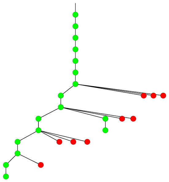
Figure 4. The search tree for the Cremona–Richmond configuration.

Since isomorphism testing is quite expensive, we utilize a simple trick (called isomorph-rejector-borders) that empirically reduces the computing time. This trick is applied on the second part of the algorithm, namely the isomorph rejector. We can think of this trick as a delayed isomorphism test. Keeping in mind that isomorphism testing via canonical forms is more expensive than the testing of the combinatorial conditions (I)–(IV), we try to increase the number of nodes which are eliminated by the “cheap” combinatorial tests. One could also say that since most of the search nodes in the search space do not complete anyway, it may not be worth the effort to perform isomorphism testing on all such nodes. Indeed, the isomorphism testing seems to be worth the effort mostly in the early stages (rows) in the search, as it keeps down the number of possible considered nodes in the search tree. Therefore, it reduces the size of the search space. However, at later stages in the search tree, many partial geometries do not lift, so it is better to eliminate these nodes by means of the combinatorial testing only. So, the isomorph-rejector-borders interval is of the form $[a,b]$ for $0\le a<b\le v.$ Outside this interval, the regular isomorph rejection takes place. However, inside the interval, isomorph rejection is performed only for those nodes that possess an extension to level $b.$ This means that nodes that do not complete are eliminated based on the combinatorial conditions (I)–(IV) only, not by the isomorph rejection. The interval is chosen by experimentation; see Table 8. Indeed, once the search tree reaches a node at level b, we perform the outstanding isomorphism tests at all intermediate levels from a to b in increasing order. This ensures that the resulting objects are pairwise non-isomorphic. Empirically, this trick saves us a lot of time in the search.

Table 8. The isomorph rejector border intervals.

Case	[a, b]
${23}_3$	[18, 22]
${24}_3$	[19, 23]

Applying the algorithm described above with the isomorph-rejector-borders trick, we classified the TFC ${23}_3$ in about 66 hours of CPU time (on a single CPU machine handling eight separate jobs). On the same machine, the search for TFC ${24}_3$ was completed in about 456 days of CPU time. The complexity of our algorithm (to compute the lexicographically least representative of the isomorphism class of a matrix) is exponential in the size of the input. A polynomial time algorithm to solve the canonical form testing problem is unknown.

9. Some Specific Examples

In this section we present the main results of the search for TFC $v_3$ for $v=23$ and 24. We also provide some properties and details about these configurations.

We will display a TFC $v_3$ configurations by listing the blocks in a tabular format. We write $1,2,\dots ,v$ for points and we write $l_1,l_2,\dots ,l_v$ for blocks (or lines). We also write ago to denote the automorphism group order.

In Table 9 and Table 10, an entry $a\times b$ means that the number of TFC $v_3$ configurations with automorphism group of order b is exactly a.

Table 9. Distribution of the automorphism group orders for TFC ${23}_3$.

5,176,505 × 1	699 × 4	10 × 12
24,700 × 2	20 × 6	3 × 16
89 × 3	67 × 8	2 × 24

Table 10. Distribution of the automorphism group orders for TFC ${24}_3$.

163,202,585 × 1	133 × 6	4 × 16	2 × 36
144,358 × 2	35 × 8	1 × 24	2 × 48
370 × 3	21 × 12	2 × 32	1 × 144
685 × 4

An entry $x\left(y\right)$ in Table 11 and Table 12 in the column “Order” indicates that there are y automorphism groups of order x.

Table 11. The automorphism group types for TFC ${23}_3$ excluding both trivial and prime order groups.

Order	Type of Group	Order	Type of Group
4 (631)	$C_2\times C_2$	8 (37)	$D_4$
4 (68)	$C_4$	12 (2)	$A_4$
6 (4)	$C_6$	12 (8)	$D_6$
6 (16)	$S_3$	16 (2)	$C_2\times D_4$
8 (20)	$C_2\times C_2\times C_2$	16 (1)	$D_8$
8 (10)	$C_4\times C_2$	24 (2)	$S_4$

Table 12. The automorphism group types for TFC ${24}_3$ excluding both trivial and prime order groups.

Order	Type of Group	Order	Type of Group
4 (633)	$C_2\times C_2$	16 (1)	$C_2\times D_4$
4 (52)	$C_4$	16 (2)	${\mathrm{QD}}_8$
6 (18)	$C_6$	16 (1)	$D_8$
6 (115)	$S_3$	24 (1)	$D_{12}$
8 (4)	$C_4\times C_2$	32 (2)	$(C_2\times D_4)$:$C_2$
8 (9)	$C_8$	36 (2)	$S_3\times S_3$
8 (22)	$D_4$	48 (1)	$(C_3\times D_4)$:$C_2$
12 (1)	$C_{12}$	48 (1)	$\mathrm{SL}(2,3)$:$C_2$
12 (20)	$D_6$	144 (1)	$(C_3\times SL(2,3))$:$C_2$

9.1. Triangle-Free 23₃ Configurations

There are exactly 5,202,095 non-isomorphic TFC ${23}_3$. The distribution of the automorphism group orders is presented in Table 9.

The types of non-trivial automorphism groups (of order other than a prime) are presented in Table 11. We use $C_n$, $D_n$, $A_n$, and $S_n$ to denote the cyclic group of order n, the dihedral group of order $2n$, the alternating group of order n, and the symmetric group of order n, respectively.

According to Table 5, there are no TFC ${23}_3$ with point, line or flag-transitive automorphism groups. There are 13,095 self-dual TFC ${23}_3$. Among those, there are exactly 13,082 self-polar TFC ${23}_3$. The 13 TFC ${23}_3$ that are self-dual but are not self-polar are all of ago 2, except two structures. One of which is the unique TFC ${23}_3$ with automorphism group $C_2\times C_2$ of order 4 and the other is the unique TFC ${23}_3$ with automorphism group $C_2\times D_4$ of order 16.

One of the 37 TFC ${23}_3$ with automorphism group $D_4$ is the geometric triangle-free ${23}_3$ configuration ${\mathcal{C}}_1$ from [36]. It is of orbit type $(6,5)$, and its age is 8.

The search for triangle-free ${23}_3$ configurations was performed on a single CPU machine split into eight jobs. Overall, the search was performed in (about) 66 hours.

9.1.1. The Unique Self-Dual but Not Self-Polar Example with Ago 4

There are 699 TFC ${23}_3$ with automorphism group of order 4. Exactly one configuration is self-dual but not self-polar. The blocks of this TFC ${23}_3$ with ago 4 are:

$l_1$	$l_2$	$l_3$	$l_4$	$l_5$	$l_6$	$l_7$	$l_8$	$l_9$	$l_{10}$	$l_{11}$	$l_{12}$	$l_{13}$	$l_{14}$	$l_{15}$	$l_{16}$	$l_{17}$	$l_{18}$	$l_{19}$	$l_{20}$	$l_{21}$	$l_{22}$	$l_{23}$
1	1	1	2	2	3	3	4	4	5	5	6	6	7	7	12	12	13	13	14	14	15	15
2	4	6	8	10	12	14	8	10	9	11	8	11	9	10	16	17	19	20	16	18	17	21
3	5	7	9	11	13	15	16	17	18	19	20	21	22	23	21	18	22	23	19	23	20	22

The automorphism group is generated by a and b where

$$\begin{array}{cc}\hfill a& =(4,5)(6,7)(8,9)(10,11)(12,14)(13,15)(16,18)(17,19)(20,22)(21,23),\hfill \\ \hfill b& =(4,6)(5,7)(10,11)(12,15)(13,14)(16,20)(17,21)(18,22)(19,23).\hfill \end{array}$$

It is of orbit type 9. It has nine point-orbits of three different sizes:

$$\left\{1\right\},\left\{2\right\},\left\{3\right\},\{4,5,6,7\},\{8,9\},\{10,11\},\{12,13,14,15\},\{16,18,20,22\},\{17,19,21,23\}.$$

9.1.2. The Unique Self-Dual Not Self-Polar Example with Ago 16

There are exactly 3 TFC ${23}_3$ with ago 16. Exactly one TFC ${23}_3$ with ago 16 is self-dual but not self-polar. The blocks of this unique self-dual not self-polar TFC ${23}_3$ with ago 16 are:

$l_1$	$l_2$	$l_3$	$l_4$	$l_5$	$l_6$	$l_7$	$l_8$	$l_9$	$l_{10}$	$l_{11}$	$l_{12}$	$l_{13}$	$l_{14}$	$l_{15}$	$l_{16}$	$l_{17}$	$l_{18}$	$l_{19}$	$l_{20}$	$l_{21}$	$l_{22}$	$l_{23}$
1	1	1	2	2	3	3	4	4	5	5	6	6	7	7	12	12	13	13	14	14	15	15
2	4	6	8	10	12	14	8	10	9	11	8	10	9	11	16	17	18	19	16	20	17	21
3	5	7	9	11	13	15	16	17	18	19	20	21	22	23	22	23	20	21	19	23	18	22

The automorphism group is generated by a, b, c and d where

$$\begin{array}{cc}\hfill a& =(8,10)(9,11)(14,15)(16,17)(18,19)(20,21)(22,23),\hfill \\ \hfill b& =(4,5)(6,7)(8,9)(10,11)(12,13)(14,15)(16,18)(17,19)(20,22)(21,23),\hfill \\ \hfill c& =(4,6)(5,7)(12,13)(16,20)(17,21)(18,22)(19,23),\hfill \\ \hfill d& =(1,2)(4,8)(5,9)(6,10)(7,11)(12,14)(13,15)(17,20)(19,22).\hfill \end{array}$$

It is of orbit type 5. It has five point-orbits of four different sizes:

$$\{1,2\},\left\{3\right\},\{4,5,6,7,8,9,10,11\},\{12,13,14,15\},\{16,17,18,19,20,21,22,23\}.$$

9.1.3. The Unique TFC ${23}_3$ with Automorphism Group $D_8$

There is a unique TFC ${23}_3$ with automorphism group $D_8$ of order 16, see Figure 5. This TFC ${23}_3$ is self-polar. The blocks of this unique self-dual and self-polar TFC ${23}_3$ with ago 16 are:

$l_1$	$l_2$	$l_3$	$l_4$	$l_5$	$l_6$	$l_7$	$l_8$	$l_9$	$l_{10}$	$l_{11}$	$l_{12}$	$l_{13}$	$l_{14}$	$l_{15}$	$l_{16}$	$l_{17}$	$l_{18}$	$l_{19}$	$l_{20}$	$l_{21}$	$l_{22}$	$l_{23}$
1	1	1	2	2	3	3	4	4	5	5	6	6	7	7	12	12	13	13	14	14	15	15
2	4	6	8	10	12	14	8	10	9	11	8	11	9	10	16	17	20	21	16	18	17	19
3	5	7	9	11	13	15	16	17	18	19	20	21	22	23	19	18	23	22	22	20	21	23

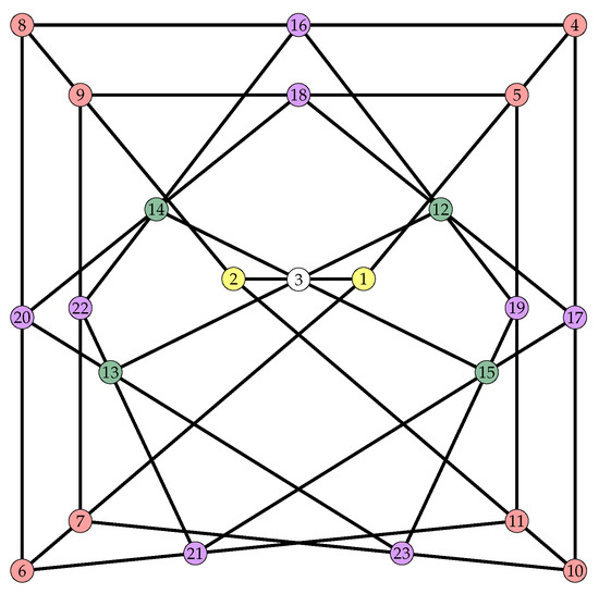
Figure 5. The Unique self-dual and self-polar TFC ${23}_3$ whose automorphism group is $D_8$ of order 16. The colored nodes correspond to the five point-orbits of the configuration.

The automorphism group is generated by a, b, c and d where

$$\begin{array}{cc}\hfill a& =(6,7)(8,10)(9,11)(14,15)(16,17)(18,19)(20,23)(21,22),\hfill \\ \hfill b& =(4,5)(6,7)(8,9)(10,11)(16,18)(17,19)(20,22)(21,23),\hfill \\ \hfill c& =(4,6)(5,7)(10,11)(12,13)(16,20)(17,21)(18,22)(19,23),\hfill \\ \hfill d& =(1,2)(4,8)(5,9)(6,10)(7,11)(12,14)(13,15)(17,20)(19,22)(21,23).\hfill \end{array}$$

It is of orbit type 5. It has five point-orbits of four different sizes:

$$\{1,2\},\left\{3\right\},\{4,5,6,7,8,9,10,11\},\{12,13,14,15\},\{16,17,18,19,20,21,22,23\}.$$

9.2. Triangle-Free 24₃ Configurations

There are exactly 163,348,199 non-isomorphic TFC ${24}_3$. The distribution of the automorphism groups’ order is presented in Table 10.

The types of non-trivial automorphism groups (of order other than a prime) are presented in Table 12. For groups A and B, we write A:B to denote a split extension of A by B (A is a normal subgroup). We also write ${\mathrm{QD}}_n$ and $\mathrm{SL}(d,q)$ to denote the quasi-dihedral group of order $2n$ and the special linear group of all $d\times d$ matrices over a finite field with q elements, respectively.

Table 5 implies that there is exactly one flag-transitive triangle-free configuration ${24}_3$, with age $144.$ From Table 12 it follows that there are two triangle-free configurations with ${24}_3$ with a group of order 48. They are not flag-transitive.

There are 84,633 self-dual TFC ${24}_3$. Among those, there are exactly 84,593 self-polar TFC ${24}_3$. The 40 TFC ${24}_3$ that are self-dual but are not self-polar are all of ago 2, except for four configurations of ago 4.

The search for triangle-free ${24}_3$ configurations was performed on a single CPU machine but split into 100 jobs. Overall, the search consumed about 456 days of CPU time.

9.2.1. TFC ${24}_3$ with Automorphism Group Order 12

There are exactly 21 TFC ${24}_3$ with automorphism group order 12. Among these there are 20 TFC ${24}_3$ whose automorphism group is $D_6$. The unique remaining TFC ${24}_3$ is the one with automorphism group $C_{12}$. We present here the unique TFC ${24}_3$ with automorphism group $C_{12}$ of order 12, see Figure 6. The blocks of this TFC ${24}_3$ are described below.

$l_1$	$l_2$	$l_3$	$l_4$	$l_5$	$l_6$	$l_7$	$l_8$	$l_9$	$l_{10}$	$l_{11}$	$l_{12}$	$l_{13}$	$l_{14}$	$l_{15}$	$l_{16}$	$l_{17}$	$l_{18}$	$l_{19}$	$l_{20}$	$l_{21}$	$l_{22}$	$l_{23}$	$l_{24}$
1	1	1	2	2	3	3	4	4	5	5	6	6	7	7	9	10	11	11	12	13	13	15	18
2	4	6	8	10	12	14	8	17	9	10	8	21	14	17	21	14	15	16	20	17	19	19	21
3	5	7	9	11	13	15	16	18	19	12	20	22	16	23	23	18	22	24	23	22	24	20	24

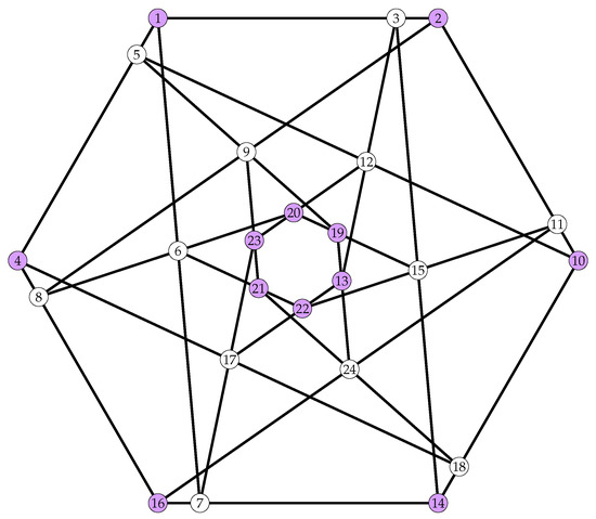
Figure 6. The Unique TFC ${24}_3$ whose automorphism group is $C_{12}$ of order 12. The two point-orbits are presented by two different colors.

The automorphism group is generated by a and b where

$$\begin{array}{cc}\hfill a& =(1,2,10,14,16,4)(3,11,18,7,8,5)(6,9,12,15,24,17)(13,22,21,23,20,19),\hfill \\ \hfill b& =(1,13,4,19,16,20,14,23,10,21,2,22)(3,17,5,24,8,15,7,12,18,9,11,6).\hfill \end{array}$$

It is of orbit type 2. It has two point-orbits of the same size,

$$\{1,2,4,10,13,14,16,19,20,21,22,23\},\{3,5,6,7,8,9,11,12,15,17,18,24\}.$$

9.2.2. The Unique TFC ${24}_3$ with Ago 24

There is a unique TFC ${24}_3$ with automorphism group order 24, see Figure 7. Its automorphism group is $D_{12}$. It is self-dual and self-polar. The blocks of this unique TFC ${24}_3$ with ago are described below.

$l_1$	$l_2$	$l_3$	$l_4$	$l_5$	$l_6$	$l_7$	$l_8$	$l_9$	$l_{10}$	$l_{11}$	$l_{12}$	$l_{13}$	$l_{14}$	$l_{15}$	$l_{16}$	$l_{17}$	$l_{18}$	$l_{19}$	$l_{20}$	$l_{21}$	$l_{22}$	$l_{23}$	$l_{24}$
1	1	1	2	2	3	3	4	4	5	5	6	6	7	7	8	9	10	11	11	13	15	16	20
2	4	6	8	10	12	14	8	12	10	19	9	13	14	17	20	15	14	12	16	23	18	18	21
3	5	7	9	11	13	15	16	17	18	20	19	21	22	23	24	17	24	19	22	24	21	23	22

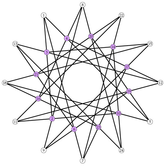
Figure 7. The Unique TFC ${24}_3$ whose automorphism group is $D_{12}$ of order 24. The two point-orbits are presented by two different colors.

The automorphism group is generated by a, b and c where

$$\begin{array}{cc}\hfill a& =(2,3)(4,6)(5,7)(8,13)(9,12)(10,14)(11,15)(16,21)(17,19)(18,22)(20,23),\hfill \\ \hfill b& =(1,12,9)(2,4,19)(3,17,6)(5,11,8)(7,13,15)(10,16,20)(14,23,21)(18,22,24),\hfill \\ \hfill c& =(1,5,18,15,9,8,24,13,12,11,22,7)(2,20,23,3,19,16,14,6,4,10,21,17).\hfill \end{array}$$

It is of orbit type 2. It has two point-orbits of the same size,

$$\{1,5,7,8,9,11,12,13,15,18,22,24\},\{2,3,4,6,10,14,16,17,19,20,21,23\}.$$

9.2.3. Two TFC ${24}_3$ with Ago 48

There are two TFC ${24}_3$ with automorphism group order 48. Their automorphism groups as listed in Table 12 are $(C_3\times D_4)$:$C_2$ and $SL(2,3)$:$C_2$. Both of these structures are point-transitive and block-transitive.

The blocks of the TFC ${24}_3$ with automorphism group $(C_3\times D_4):C_2$ are

$l_1$	$l_2$	$l_3$	$l_4$	$l_5$	$l_6$	$l_7$	$l_8$	$l_9$	$l_{10}$	$l_{11}$	$l_{12}$	$l_{13}$	$l_{14}$	$l_{15}$	$l_{16}$	$l_{17}$	$l_{18}$	$l_{19}$	$l_{20}$	$l_{21}$	$l_{22}$	$l_{23}$	$l_{24}$
1	1	1	2	2	3	3	4	4	5	5	6	6	7	7	8	9	10	11	11	13	14	15	20
2	4	6	8	10	12	14	8	12	10	19	9	13	14	17	20	15	21	12	16	18	16	21	23
3	5	7	9	11	13	15	16	17	18	20	19	21	22	23	22	17	22	19	24	23	18	24	24

While the blocks of the TFC ${24}_3$ with automorphism group $SL(2,3)$:$C_2$ are

$l_1$	$l_2$	$l_3$	$l_4$	$l_5$	$l_6$	$l_7$	$l_8$	$l_9$	$l_{10}$	$l_{11}$	$l_{12}$	$l_{13}$	$l_{14}$	$l_{15}$	$l_{16}$	$l_{17}$	$l_{18}$	$l_{19}$	$l_{20}$	$l_{21}$	$l_{22}$	$l_{23}$	$l_{24}$
1	1	1	2	2	3	3	4	4	5	5	6	6	7	7	8	9	10	11	11	13	15	18	20
2	4	6	8	10	12	14	8	12	10	19	9	14	13	19	14	17	12	15	17	21	22	22	21
3	5	7	9	11	13	15	16	17	18	20	18	21	16	22	19	20	23	16	24	24	23	24	23

Figure 8 presents the Levi graphs of those two TFC ${24}_3$, while Figure 9 presents the two TFC ${24}_3$.

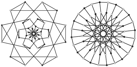
Figure 8. The Levi graphs of the two TFC ${24}_3$ whose automorphism groups are $(C_3\times D_4)$:$C_2$ (left) and $SL(2,3)$:$C_2$ (right) of order 48. The points and lines of each configuration are presented by black nodes and white nodes, respectively.

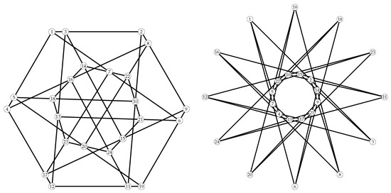
Figure 9. The two point-transitive TFC ${24}_3$ whose automorphism groups are $(C_3\times D_4)$:$C_2$ (left) and $SL(2,3)$:$C_2$ (right) of order 48.

Both configurations are self-dual and self-polar. In Figure 8, a polarity can be found by reversing the role of points and blocks with the mapping $p_i\leftrightarrow B_i$ for $i=1,2,\cdots ,24$ on the Levi graph.

9.2.4. The Unique TFC ${24}_3$ with Ago 144

There is a unique TFC ${24}_3$ with automorphism group order 144. Its automorphism group listed in Table 12 is $(C_3\times SL(2,3))$:$C_2$. It is also an example of a self-dual and self-polar configuration. The blocks of this unique TFC ${24}_3$ with ago 144 are

$l_1$	$l_2$	$l_3$	$l_4$	$l_5$	$l_6$	$l_7$	$l_8$	$l_9$	$l_{10}$	$l_{11}$	$l_{12}$	$l_{13}$	$l_{14}$	$l_{15}$	$l_{16}$	$l_{17}$	$l_{18}$	$l_{19}$	$l_{20}$	$l_{21}$	$l_{22}$	$l_{23}$	$l_{24}$
1	1	1	2	2	3	3	4	4	5	5	6	6	7	7	9	10	11	11	13	15	16	17	18
2	4	6	8	10	12	14	8	17	9	10	8	13	12	16	18	15	14	19	21	20	20	19	21
3	5	7	9	11	13	15	16	18	19	12	14	20	17	21	22	23	22	24	23	24	22	23	24

Figure 10 presents the Levi graphs of those two TFC ${24}_3$.

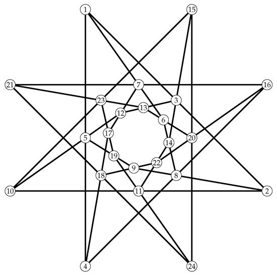
Figure 10. The Unique TFC ${24}_3$ whose automorphism group order is 144. It is also the unique flag-transitive configuration.

10. Conclusions

This paper is a contribution to the study of triangle-free configurations. These incidence structures are more restriceted than configurations, but somewhat less restricted than generalized quadrangles. We have extended the classification of these objects from order 22 to order 24. We found some interesting objects with large symmetry group.s In particular, we found one flag-transitive configuration, ${24}_3$, with an automorphism group of order 144. We discussed our algorithms for computer search and talked about related research such as realizations of configurations using straight lines in the real plane.

References

- Tits, J. Sur la trialité et certains groupes qui s’en déduisent. Inst. Hautes Études Sci. Publ. Math. 1959, 2, 13–60. [Google Scholar] [CrossRef]
- Payne, S.E.; Thas, J.A. Finite Generalized Quadrangles, 2nd ed.; EMS Series of Lectures in Mathematics; European Mathematical Society (EMS): Zürich, Switzerland, 2009; p. xii+287. [Google Scholar] [CrossRef]
- Cameron, P.J.; van Lint, J.H. Designs, Graphs, Codes and Their Links; London Mathematical Society Student Texts; Cambridge University Press: Cambridge, UK, 1991; Volume 22, p. x+240. [Google Scholar] [CrossRef]
- Karaoglu, F. Smooth cubic surfaces with 15 lines. Appl. Algebra Engrg. Comm. Comput. 2022, 33, 823–853. [Google Scholar] [CrossRef]
- Schläfli, L. An attempt to determine the twenty-seven lines upon a surface of the third order and to divide such surfaces into species in reference to the reality of the lines upon the surface. Quart. J. Math. 1858, 2, 55–110. [Google Scholar]
- Conway, J.H.; Curtis, R.T.; Norton, S.P.; Parker, R.A.; Wilson, R.A. Atlas of Finite Groups; Oxford University Press: Oxford, UK, 1985; p. xxxiv+252, Maximal subgroups and ordinary characters for simple groups, with computational assistance from J.G. Thackray. [Google Scholar]
- Dickson, L. Projective classification of cubic surfaces modulo 2. Ann. Math. 1915, 16, 139–157. [Google Scholar] [CrossRef]
- Cremona, L. Teoremi Stereometrici dal quali si Deducono le Proprietà dell’ Esagrammo di PASCAL. Atti Della R. Accad. Lincei 1877, 1, 854–874. [Google Scholar]
- Richmond, H.W. The figure formed from six points in space of four dimensions. Math. Ann. 1900, 53, 161–176. [Google Scholar] [CrossRef][Green Version]
- Martinetti, V. Sopra Alcune Configurazioni Piane. Ann. Mat. Pura Appl. 1886, 14, 161–192. [Google Scholar] [CrossRef]
- Betten, A.; Brinkmann, G.; Pisanski, T. Counting symmetric configurations v3. In Proceedings of the 5th Twente Workshop on Graphs and Combinatorial Optimization (Enschede, 1997), Enschede, The Netherlands, 24–26 June 1997; Volume 99, pp. 331–338. [Google Scholar] [CrossRef]
- Boben, M.; Grünbaum, B.; Pisanski, T.Z.; Zitnik, A. Small triangle-free configurations of points and lines. Discret. Comput. Geom. 2006, 35, 405–427. [Google Scholar] [CrossRef]
- Al-Azemi, A.; Betten, A. Classification of triangle-free 223 configurations. Int. J. Comb. 2010, 17, 767361. [Google Scholar] [CrossRef]
- Grünbaum, B. Configurations of points and lines. In Graduate Studies in Mathematics; American Mathematical Society: Providence, RI, USA, 2009; Volume 103, p. xiv+399. [Google Scholar] [CrossRef]
- Saniga, M. The Complement of Binary Klein Quadric as a Combinatorial Grassmannian. Mathematics 2015, 3, 481–486. [Google Scholar] [CrossRef]
- Cremona, L. Mémoire de géométrie pure sur les surfaces du troisième ordre. J. Reine Angew. Math. 1868, 68, 1–133. [Google Scholar] [CrossRef]
- Planat, M.; Zainuddin, H. Zoology of Atlas-Groups: Dessins D’enfants, Finite Geometries and Quantum Commutation. Mathematics 2017, 5, 6. [Google Scholar] [CrossRef]
- Dembowski, P. Finite Geometries; Classics in Mathematics; Springer: Berlin/Heidelberg, Germany, 1997; p. xii+375, Reprint of the 1968 original. [Google Scholar]
- Block, R.E. On automorphism groups of block designs. J. Comb. Theory 1968, 5, 293–301. [Google Scholar] [CrossRef]
- Betten, A. Large Sets of Desargues Configurations. In Proceedings of the 5th Pythagorean Conference, Kalamata, Greece, 1–6 June 2025. to appear, 2025+. [Google Scholar]
- Coxeter, H.S.M. Self-dual configurations and regular graphs. Bull. Amer. Math. Soc. 1950, 56, 413–455. [Google Scholar] [CrossRef]
- Tutte, W.T. The chords of the non-ruled quadric in PG(3, 3). Can. J. Math. 1958, 10, 481–483. [Google Scholar] [CrossRef]
- Coxeter, H.S.M. The chords of the non-ruled quadric in PG(3, 3). Can. J. Math. 1958, 10, 484–488. [Google Scholar] [CrossRef]
- Grünbaum, B. Geometric Realization of Some Triangle-Free Combinatorial Configurations 223. Int. Sch. Res. Not. 2012, 2012, 560760. [Google Scholar] [CrossRef][Green Version]
- Bokowski, J.; Pilaud, V. Enumerating topological (nk)-configurations. Comput. Geom. 2014, 47, 175–186. [Google Scholar] [CrossRef]
- Bokowski, J.; Sturmfels, B. Computational Synthetic Geometry; Lecture Notes in Mathematics; Springer: Berlin/Heidelberg, Germany, 1989; Volume 1355, p. vi+168. [Google Scholar] [CrossRef]
- Bokowski, J.; Pilaud, V. On topological and geometric (194) configurations. Eur. J. Comb. 2015, 50, 4–17. [Google Scholar] [CrossRef]
- Sturmfels, B.; White, N. All 113 and 123-configurations are rational. Aequationes Math. 1990, 39, 254–260. [Google Scholar] [CrossRef]
- Faradžev, I.A. Constructive enumeration of combinatorial objects. In Problèmes Combinatoires et Théorie des Graphes; CNRS: Paris, France, 1978; Volume 260, pp. 131–135. [Google Scholar]
- Read, R.C. Every one a winner or how to avoid isomorphism search when cataloguing combinatorial configurations. Ann. Discret. Math. 1978, 2, 107–120. [Google Scholar]
- McKay, B. Nauty and Traces, version 2.7r1; Australian National University: Canberra, Australia, 2020.
- McKay, B.D. Isomorph-free exhaustive generation. J. Algorithms 1998, 26, 306–324. [Google Scholar] [CrossRef]
- McKay, B.D.; Piperno, A. Practical graph isomorphism, II. J. Symbolic Comput. 2014, 60, 94–112. [Google Scholar] [CrossRef]
- Betten, A. The Orbiter Ecosystem for Combinatorial Objects. In Proceedings of the ISSAC 2020, International Symposium on Symbolic and Algebraic Computation, Kalamazoo, MI, USA, 20–23 July 2020; ACM: New York, NY, USA, 2020; pp. 30–37. [Google Scholar] [CrossRef]
- Kaski, P.; Östergård, P. Classification Algorithms for Codes and Designs. In Algorithms and Computation in Mathematics; Springer: Berlin/Heidelberg, Germany, 2006; Volume 15. [Google Scholar]
- Raney, M.W. On geometric trilateral-free (n3) configurations. Ars Math. Contemp. 2013, 6, 253–259. [Google Scholar] [CrossRef]
Disclaimer/Publisher’s Note: The statements, opinions and data contained in all publications are solely those of the individual author(s) and contributor(s) and not of MDPI and/or the editor(s). MDPI and/or the editor(s) disclaim responsibility for any injury to people or property resulting from any ideas, methods, instructions or products referred to in the content. |
© 2025 by the authors. Licensee MDPI, Basel, Switzerland. This article is an open access article distributed under the terms and conditions of the Creative Commons Attribution (CC BY) license (https://creativecommons.org/licenses/by/4.0/).