Covariate-Adjusted Precision Matrix Estimation Under Lower Polynomial Moment Assumption

Abstract

Multiple regression analysis has a wide range of applications. The analysis of error structures in regression model $\mathit{Y}=\mathbf{\Gamma }\mathit{X}+\mathit{Z}$ has also attracted much attention. This paper focuses on large-scale precision matrix of the error vector that only has lower polynomial moments. We mainly study upper bounds of the proposed estimator under different norms in term of the probability estimation. It is shown that our estimator achieves the same optimal convergence order as under Gaussian assumption on the data. Simulation experiments further validate that our method has advantages.

1. Introduction

Multivariate regression methods are growing increasingly important in numerous fields, including chemometrics [1], neuroscience [2], genomics [3], and finance [4]. In genomics research, multivariate models connect gene expression $\mathit{Y}$ to genetic variants $\mathit{X}$ and infer gene regulatory networks via Gaussian graphical models (GGMs)—a process that relies heavily on precision matrices. As emphasized by Liu and Yu [5], the error structure (closely linked to precision matrices) of the multivariate linear regression model for responses, $\mathit{Y}=\mathbf{\Gamma }\mathit{X}+\mathit{Z}$, is critical for reliable inference but often overlooked in high dimensions settings. Compared with the covariance matrix, the precision matrix of the random error $\mathit{Z}$ is more directly interpretable (e.g., it captures conditional dependence relationships in gene networks) and more relevant to practical applications, thus attracting considerable research attention.

Cai et al. [6] proposed CLIME (Constrained $l_1$ Minimization Estimation) method for precision matrix and obtained probability estimation under exponential and polynomial moment conditions, respectively. Cai et al. [7] further developed the ACLIME (Adaptive Constrained $l_1$ Minimization Estimation) method and established optimal convergence rate for precision matrix under Gaussian assumption on the data. By replacing the sample covariance matrix with a pilot estimator, Avella-Medina et al. [8] discussed optimal precision matrix estimation under finite 2 + $\epsilon$ moment condition. This robust estimation framework focuses on independent random vectors, meaning it cannot address the coupling between regression effects and error structures.

While these methods have achieved notable progress in precision matrix estimation, their frameworks primarily focus on single random vectors (e.g., univariate responses) and fail to account for regression relationships between multiple variables. Cai et al. [9] proposed a two-stage constrained $l_1$ minimization approach to estimate the coefficient matrix and the precision matrix of sub-Gaussian error $\mathit{Z}$, which means the data requires finite moments of any order. Chen et al. [10] used a scaled Lasso and pairwise regression strategy to estimate these two matrices, which considers Gaussian data and does not provide any convergence rate. Ten et al. [11] developed a bias-corrected method to estimate the covariance matrix of the error vector $\mathit{Z}$, but this method cannot infer the conditional independence between error variables. Additionally, its robustness is based on the Gaussian distribution framework, making it inadequate for in-depth analysis of error structures in non-Gaussian scenarios.

This paper adopts a two-stage constrained $l_1$ minimization method to investigate probability precision matrix estimation for error vectors that only possess $4\gamma +4+\epsilon (\gamma ,\epsilon >0)$ order moment. Our theoretical results demonstrate that the proposed estimator not only achieves the same convergence rate as Cai et al.’s method but also exhibits superior numerical performance.

Throughout this paper, we use $X\lesssim Y$ to denote $X\le CY$ for some positive constant C, and $X\gtrsim Y$ denotes $Y\lesssim X$. For a vector $\mathit{\beta }={\left({\beta }_1,\dots ,{\beta }_p\right)}^T\in {\mathbb{R}}^p$, we define ${\parallel \mathit{\beta }\parallel }_1={\displaystyle \sum _{i=1}^p}\left|{\beta }_i\right|$ and ${\parallel \mathit{\beta }\parallel }_{\infty }=\underset{i}{max}\left|{\beta }_i\right|$. For a matrix $\mathit{A}=\left(a_{ij}\right)\in R^{p\times q}$, ${\parallel \mathit{A}\parallel }_{max}=\underset{ij}{max}|a_{ij}|$, ${\parallel \mathit{A}\parallel }_{l_1}=\underset{1\le j\le q}{max}{\displaystyle \sum _{i=1}^p}\left|a_{ij}\right|$, ${\parallel \mathit{A}\parallel }_{l_{\infty }}=\underset{1\le i\le p}{max}{\displaystyle \sum _{j=1}^q}\left|a_{ij}\right|$, ${\parallel \mathit{A}\parallel }_1={\displaystyle \sum _{i=1}^p}{\displaystyle \sum _{j=1}^q}|a_{ij}|$, ${\parallel \mathit{A}\parallel }_F=({\displaystyle \sum _{i=1}^p}{\displaystyle \sum _{j=1}^q}|a_{ij}{{|}^2)}^{1/2}$ and ${\parallel \mathit{A}\parallel }_2$ stands for the spectrum norm of a matrix $\mathit{A}$.

The rest is organized as follows. Section 2 details the construction of the proposed estimator; Section 3 presents the theoretical properties of the estimator; Section 4 reports simulation studies and an analysis of human gut microbiome data; Section 5 provides discussions. All technical proofs are included in Appendix A.

2. Preliminaries

We begin with a genetical genomics dataset. Let $\mathit{Y}={(Y_1,\cdots ,Y_p)}^T$ be a p-dimensional random vector of gene expressions and $\mathit{X}={(X_1,\cdots ,X_q)}^T$ be a q-dimensional random vector of genetic markers. We consider the following multiple regression model:

$$\mathit{Y}=\mathbf{\Gamma }\mathit{X}+\mathit{Z},$$

(1)

where $\mathbf{\Gamma }\in {\mathbb{R}}^{p\times q}$ is an unknown coefficient matrix. The random vector $\mathit{Z}={(Z_1,\cdots ,Z_p)}^T$ has a mean of $\mathbf{0}$, a covariance matrix $\mathbf{\Sigma }=\left({\sigma }_{ij}\right)=\mathbb{E}\mathit{Z}{\mathit{Z}}^T$, and a precision matrix $\mathbf{\Omega }={\mathbf{\Sigma }}^{-1}=\left({\omega }_{ij}\right)=({\mathit{\omega }}_1,\cdots ,{\mathit{\omega }}_p)$. Assuming that $\mathit{X}$ and $\mathit{Z}$ are independent, we observe n to be independent and identically distributed (i.i.d) random samples $({\mathit{X}}_1,{\mathit{Y}}_1),\cdots ,({\mathit{X}}_n,{\mathit{Y}}_n)$ generated from the model (1). Accordingly, the samples of $\mathit{Z}$ can be derived from the model (1).

In genomic studies, the coefficient matrix $\mathbf{\Gamma }$ in the model (1) is sparse, as each gene is typically regulated by only a small number of genetic regulators. Similarly, the precision matrix $\mathbf{\Omega }$ is expected to be sparse, reflecting the fact that genetic interaction networks generally exhibit limited connectivity. Motivated by these sparsity properties and the need to establish rigorous convergence rates for estimators, we introduce the following conditions.

Condition 1.

For some constants $\gamma ,c>0$, the dimensions satisfy $(p\vee q)\le c{n}^{\gamma }$, where $p\vee q=max\{p,q\}$. Additionally, there exist constants $\epsilon >0$ and $K>0$ such that

$$\underset{1\le i\le q}{max}\mathbb{E}|X_i{|}^{4\gamma +4+\epsilon }\le K,\underset{1\le i\le p}{max}\mathbb{E}|Z_i{|}^{4\gamma +4+\epsilon }\le K,\underset{1\le j\le p}{max}\mathbb{E}{|{\mathit{Z}}^T{\mathit{\omega }}_j|}^{4\gamma +4+\epsilon }\le K.$$

Condition 2.

The regression coefficient matrix $\mathbf{\Gamma }\in {\mathcal{V}}_{{\delta }_1}\left(s_1\left(q\right)\right)$ with $0⩽{\delta }_1<1$, where

$${\mathcal{V}}_{{\delta }_1}\left(s_1\left(q\right)\right)=\{\mathbf{\Gamma }\in {\mathbb{R}}^{p\times q}:\underset{1⩽i⩽p}{max}{\displaystyle \sum _{j=1}^q}{\left|{\gamma }_{ij}\right|}^{{\delta }_1}⩽s_1\left(q\right)\}.$$

Condition 3.

The precision matrix $\mathbf{\Omega }={\left({\omega }_{ij}\right)}_{p\times p}\in {\mathcal{U}}_{{\delta }_2}\left(s_2\left(p\right)\right)$ with $0⩽{\delta }_2<1$, where

$$\begin{array}{c}{\mathcal{U}}_{{\delta }_2}\left(s_2\left(p\right)\right)=\{\mathbf{\Omega }>0:{\parallel \mathbf{\Omega }\parallel }_{l_{\infty }}⩽M_p,{\displaystyle \underset{1⩽i⩽p}{max}}{\displaystyle \sum _{j=1}^p}{\left|{\omega }_{ij}\right|}^{{\delta }_2}⩽s_2\left(p\right)\}.\end{array}$$

Condition 4.

There exists some $N_q>0$ such that ${\parallel {\mathbf{\Sigma }}_{\mathit{X}}^{-1}\parallel }_{l_{\infty }}⩽N_q$, where ${\mathbf{\Sigma }}_{\mathit{X}}$ is the covariance matrix of $\mathit{X}$.

Remark 1.

Condition 1 imposes a polynomial moment constraint on $\mathit{X}$, $\mathit{Z}$, and ${\mathit{Z}}^T{\mathit{\omega }}_j$. This condition is weaker than the sub-Gaussian moment assumption adopted by Cai et al. [9], as sub-Gaussian random variables require finite moments of all orders. The dimension growth constraint $(p\vee q)\le c{n}^{\gamma }$ implies that the growth rates of p and q are controlled by a polynomial function $n^{\gamma }$ of the sample size n, with γ governing the maximum allowable growth rate of the dimensions relative to n.

Conditions 2 and 3 formalize the sparsity assumptions for Γ and Ω, respectively, where $s_1\left(q\right)$ and $s_2\left(p\right)$ represent the sparse measurements. Under the dimension growth constraint in Condition 1, it follows that $log\left(pq\right)=o\left(n\right)$. This ensures that the sparsity measures $s_1\left(q\right)$, $s_2\left(p\right)$ and the convergence rates of the proposed estimators are all consistent with the polynomial growth of dimensions (see Theorems 2 and 3). Similar parameter spaces have been adopted in Bickel and Levina [12], Cai et al. [6] and Avella-Medina et al. [8]. However, our framework imposes no eigenvalue restrictions.

Note that ${\mathbf{\Sigma }}_X^{-1}$ corresponds to the precision matrix of $\mathit{X}$, so the constraint in Condition 4 is analogous to the bounded norm assumption for Ω in Condition 3.

The following details the construction process of the proposed estimators.

Using the independent and identically distributed random samples $({\mathit{X}}_1,{\mathit{Y}}_1),\cdots ,({\mathit{X}}_n,{\mathit{Y}}_n)$, we define the sample means as $\overline{\mathit{X}}=1/n{\sum }_{k=1}^n{\mathit{X}}_k$, $\overline{\mathit{Y}}=1/n{\sum }_{k=1}^n{\mathit{Y}}_k$ and $\overline{\mathit{Z}}=1/n{\sum }_{k=1}^n{\mathit{Z}}_k$. From the model (1), it follows that

$${\mathit{Y}}_k-\overline{\mathit{Y}}=\mathbf{\Gamma }({\mathit{X}}_k-\overline{\mathit{X}})+{\mathit{Z}}_k-\overline{\mathit{Z}}.$$

Similar to the sample covariance matrix, we define the following sample matrix, ${\widehat{\mathbf{\Sigma }}}_{\mathit{Y}\mathit{X}}:=1/n{\sum }_{k=1}^n({\mathit{Y}}_k-\overline{\mathit{Y}}){({\mathit{X}}_k-\overline{\mathit{X}})}^T$, ${\widehat{\mathbf{\Sigma }}}_{\mathit{X}\mathit{X}}:=1/n{\sum }_{k=1}^n({\mathit{X}}_k-\overline{\mathit{X}}){({\mathit{X}}_k-\overline{\mathit{X}})}^T$ and ${\widehat{\mathbf{\Sigma }}}_{\mathit{Z}\mathit{X}}:=1/n{\sum }_{k=1}^n({\mathit{Z}}_k-\overline{\mathit{Z}}){({\mathit{X}}_k-\overline{\mathit{X}})}^T$. It is straightforward to verify that ${\widehat{\mathbf{\Sigma }}}_{\mathit{Y}\mathit{X}}-\mathbf{\Gamma }{\widehat{\mathbf{\Sigma }}}_{\mathit{X}\mathit{X}}={\widehat{\mathbf{\Sigma }}}_{\mathit{Z}\mathit{X}}$.

To estimate $\mathbf{\Gamma }$ and $\mathbf{\Omega }$, we first construct an estimator for $\mathbf{\Gamma }$ via an optimization approach. Let $\widehat{\mathbf{\Gamma }}={({\widehat{\gamma }}_1,\cdots ,{\widehat{\gamma }}_p)}^T$, ${\widehat{\mathbf{\Sigma }}}_{\mathit{Y}\mathit{X}}=({\widehat{\mathbf{\Sigma }}}_{\mathit{Y}\mathit{X},1},\cdots ,{\widehat{\mathbf{\Sigma }}}_{\mathit{Y}\mathit{X},p})$. For each $j\in \{1,\cdots ,p\}$,

$${\widehat{\gamma }}_j:=arg\underset{{\mathit{\beta }}_j\in R^q}{min}\{{\parallel {\mathit{\beta }}_j\parallel }_1,{\parallel {\widehat{\mathbf{\Sigma }}}_{\mathit{Y}\mathit{X},j}-{\mathit{\beta }}_j^T{\widehat{\mathbf{\Sigma }}}_{\mathit{X}\mathit{X}}\parallel }_{max}\le {\lambda }_{n,p}\},$$

(2)

where ${\lambda }_{n,p}=C_1\sqrt{log\left(pq\right)/n}$ is a tuning parameter with a positive constant $C_1>0$. It follows that the above row-wise optimization problems are equivalent to the matrix-level optimization problem,

$$\widehat{\mathbf{\Gamma }}\in \underset{\Gamma \in {\mathbb{R}}^{p\times q}}{min}\{{\parallel \mathbf{\Gamma }\parallel }_1,\parallel {\widehat{\mathbf{\Sigma }}}_{\mathit{Y}\mathit{X}}-\mathbf{\Gamma }{\widehat{\mathbf{\Sigma }}}_{\mathit{X}\mathit{X}}{\parallel }_{max} \le {\lambda }_{n,p}\}.$$

Secondly, we construct an estimator for $\mathbf{\Omega }$. Substitute $\widehat{\mathbf{\Gamma }}$ into the model (1), and let ${\widehat{\mathbf{\Sigma }}}_{\mathit{Y}\mathit{Y}}=1/n{\sum }_{k=1}^n({\mathit{Y}}_k-\widehat{\mathbf{\Gamma }}{\mathit{X}}_k){({\mathit{Y}}_k-\widehat{\mathbf{\Gamma }}{\mathit{X}}_k)}^T$. We estimate $\mathbf{\Omega }$ by CLIME method proposed by Cai et al. [6]. Let ${\widehat{\mathbf{\Omega }}}^1:=({\widehat{\mathit{\omega }}}_1^1\cdots {\widehat{\mathit{\omega }}}_p^1)$ and

$${\widehat{\mathit{\omega }}}_j^1:=arg\underset{{\mathit{\beta }}_j\in R^p}{min}\{{\parallel {\mathit{\beta }}_j\parallel }_1,\parallel {\widehat{\mathbf{\Sigma }}}_{\mathit{Y}\mathit{Y}}{\mathit{\beta }}_j-{\mathit{e}}_j{\parallel }_{max} \le {\tau }_{n,p}\},j\in \{1,\cdots ,p\},$$

(3)

where ${\mathit{e}}_j$ is the j-th standard basis vector in ${\mathbb{R}}^p$, and ${\tau }_{n,p}=C_2\sqrt{log\left(pq\right)/n}$ is a tuning parameter with a constant $C_2>0$. We then symmetrize ${\widehat{\mathbf{\Omega }}}^1$ to obtain the final estimator $\widehat{\mathbf{\Omega }}=\left({\widehat{\omega }}_{ij}\right)$, defined as

$${\widehat{\omega }}_{ij}:={\widehat{\omega }}_{ij}^1\mathbf{1}(|{\widehat{\omega }}_{ij}^1| \le |{\widehat{\omega }}_{ji}^1|)+{\widehat{\omega }}_{ji}^1\mathbf{1}(|{\widehat{\omega }}_{ij}^1| > |{\widehat{\omega }}_{ji}^1|),$$

where $\mathbf{1}(·)$ denotes the indicator function.

Remark 2.

We obtain the proposed estimators via two key steps, corresponding to Equations (2) and (3). In the case where $q=0$, estimation of Γ is unnecessary, and the precision matrix estimator can be directly derived via (3) (CLIME, Cai et al. [6]). When $q=1$, several methods have been developed to estimate Γ, including those based on $l_1$ minimization (Tibshirani [13]) and the Dantzig selector (Candes and Tao [14]). In this paper, we consider the high-dimensional setting where both p and q may be large, but satisfy $(p\vee q)\le n^{\gamma }$ for some constant $\gamma >0$.

3. Main Result

In this section, we present our main results.

Theorem 1.

Under Condition 1, there exists a constant $C=C\left(\gamma ,\delta ,\epsilon ,K\right)>0$ such that

$$\mathbb{P}\{\parallel {\widehat{\mathbf{\Sigma }}}_{\mathit{Y}\mathit{X}}-\mathbf{\Gamma }{\widehat{\mathbf{\Sigma }}}_{\mathit{X}\mathit{X}}{\parallel }_{max} \le C\sqrt{{\displaystyle \frac{log\left(pq\right)}{n}}}\}=1-O({\left(pq\right)}^{-\delta }+n^{-\epsilon /4}),$$

(4)

$$\mathbb{P}\{\parallel {\widehat{\mathbf{\Sigma }}}_{\mathit{X}\mathit{X}}-{\mathbf{\Sigma }}_{\mathit{X}}{\parallel }_{max} \le C\sqrt{{\displaystyle \frac{log\left(pq\right)}{n}}}\}=1-O({\left(pq\right)}^{-\delta }+n^{-\epsilon /8})$$

(5)

and

$$\mathbb{P}\{\parallel {\widehat{\mathbf{\Sigma }}}_{\mathit{Z}\mathit{Z}}\mathbf{\Omega }-{\mathit{I}}_p{\parallel }_{max} \le C\sqrt{{\displaystyle \frac{log\left(pq\right)}{n}}}\}=1-O({\left(pq\right)}^{-\delta }+n^{-\epsilon /4}).$$

(6)

Remark 3.

As shown in Equation (2), Equation (4) provides the theoretical foundation for constructing the estimator $\widehat{\mathbf{\Gamma }}$. Furthermore, Equations (5) and (6) indicate that ${\widehat{\mathbf{\Sigma }}}_{\mathit{X}\mathit{X}}$ serves as a pilot estimator of the covariance matrix ${\mathbf{\Sigma }}_{\mathit{X}}$, while ${\widehat{\mathbf{\Sigma }}}_{\mathit{Z}\mathit{Z}}$ is a pilot estimator of the precision matrix Ω; see Avella-Medina et al. [8].

The following results establish error bounds for the coefficient matrix estimator $\widehat{\mathbf{\Gamma }}$ under different matrix norms.

Theorem 2.

Suppose Conditions 1, 2 and 4 hold. Let $\mathbf{\Gamma }\in {\mathcal{V}}_{{\delta }_1}\left(s_1\left(q\right)\right)$ with

$$s_1\left(q\right)=o(N_q^{{\delta }_1-1}{({\displaystyle \frac{n}{log\left(pq\right)}})}^{{\displaystyle \frac{1-\delta 2}{)}}}.$$

Then, for some constant $C=C\left(\gamma ,\delta ,\epsilon ,K\right)>0$, the estimator $\widehat{\mathbf{\Gamma }}$ defined in (2) satisfies

$$\mathbb{P}\{\parallel \widehat{\mathbf{\Gamma }}-\mathbf{\Gamma }{\parallel }_{l_{\infty }} \le C{N}_q^{1-{\delta }_1}{s}_1\left(q\right){({\displaystyle \frac{log\left(pq\right)}{n}})}^{{\displaystyle \frac{1-{\delta }_1}{2}}}\}=1-O({\left(pq\right)}^{-\delta }+n^{-\epsilon /4}),$$

(7)

$$\mathbb{P}\{\parallel \widehat{\mathbf{\Gamma }}-\mathbf{\Gamma }{\parallel }_{max} \le C{N}_q\sqrt{{\displaystyle \frac{log\left(pq\right)}{n}}}\}=1-O({\left(pq\right)}^{-\delta }+n^{-\epsilon /4})$$

(8)

and

$$\mathbb{P}\{{\displaystyle \frac{1}{p}}{\parallel \widehat{\mathbf{\Gamma }}-\mathbf{\Gamma }\parallel }_F\le C{N}_q^{2-{\delta }_1}{s}_1\left(q\right){({\displaystyle \frac{log\left(pq\right)}{n}})}^{1-{\displaystyle \frac{{\delta }_1}{2}}}\}=1-O({\left(pq\right)}^{-\delta }+n^{-\epsilon /4}).$$

(9)

Remark 4.

Since $N_q$ is bounded and $(p\vee q)\le n^{\gamma }$ implies that $\sqrt{log\left(pq\right)/n}\to 0$ as $n\to \infty$, the sparsity condition $s_1\left(q\right)=o\left(N_q^{{\delta }_1-1}{(n/log\left(pq\right))}^{(1-{\delta }_1)/2}\right)$ in Theorem 2 ensures that the upper bound of the above probability tends to zero. Moreover, since $\sqrt{n/log\left(pq\right)}\to \infty$ as $n\to \infty$, this sparsity requirement is mild.

Theorem 3.

Suppose Conditions 1–4 hold. Let $\mathbf{\Gamma }\in {\mathcal{V}}_{{\delta }_1}\left(s_1\left(q\right)\right)$ and $\mathbf{\Omega }\in {\mathcal{U}}_{{\delta }_2}\left(s_2\left(p\right)\right)$ with $s_2\left(p\right)\lesssim {(1+M_p)}^{-1}{N}_q^{{\delta }_1-2}{(n/log\left(pq\right))}^{(1-{\delta }_1)/2}$. Then, for some constant $C=C\left(\gamma ,\delta ,\epsilon ,K\right)>0$, the estimator $\widehat{\mathbf{\Omega }}$ defined in (2) satisfies

$$\mathbb{P}\{\parallel \widehat{\mathbf{\Omega }}-\mathbf{\Omega }{\parallel }_{max} \le C{M}_p\sqrt{{\displaystyle \frac{log\left(pq\right)}{n}}}\}=1-O({\left(pq\right)}^{-\delta }+n^{\epsilon /8})$$

(10)

and

$$\mathbb{P}\{\parallel \widehat{\mathbf{\Omega }}-\mathbf{\Omega }{\parallel }_2 \le C{M}_p^{1-{\delta }_2}{s}_2\left(p\right){({\displaystyle \frac{log\left(pq\right)}{n}})}^{{\displaystyle \frac{1-{\delta }_1}{2}}}\}=1-O({\left(pq\right)}^{-\delta }+n^{\epsilon /8}).$$

(11)

Remark 5.

Since $M_p$ is a positive deterministic sequence, which may be bounded or slowly diverging as n and p grow, the condition

$$s_2\left(p\right)\le C{(1+M_p)}^{-1}{N}_q^{{\delta }_1-2}{\left({\displaystyle \frac{n}{log\left(pq\right)}}\right)}^{(1-{\delta }_1)/2}$$

implies the corresponding condition in Theorem 2. Moreover, the convergence rate given in (11) matches that established by Cai et al. [9], confirming its optimality.

4. Numerical Results

4.1. Simulation Analysis

In this section, we evaluate the performance of the proposed method through simulation studies and compare it with two existing methods proposed by Cai et al. [6] and Friedman et al. [15].

For the $p\times q$ coefficient matrix $\mathbf{\Gamma }=\left({\gamma }_{ij}\right)$, the sparsity level is controlled by the parameter $s_1$. Specifically, each element ${\gamma }_{ij}$ is generated independently from $U(-1,1)\times \mathrm{Ber}(1,s_1)$, where $U(-1,1)$ denotes the uniform distribution over $[-1,1]$, and $\mathrm{Ber}(1,s_1)$ denotes a Bernoulli random variable that takes 1 with probability $s_1$ and 0 with probability $1-s_1$. This generation mechanism implies ${\gamma }_{ij}$ is non-zero with probability $s_1$ (and zero otherwise), so a smaller $s_1$ indicates a higher sparsity level for $\mathbf{\Gamma }$.

The sparsity of precision matrix $\mathbf{\Omega }=\left({\omega }_{ij}\right)$ is controlled by the parameter $s_2$. To ensure $\mathbf{\Omega }$ is positive definite, we first construct a matrix $\mathit{B}=\left(b_{ij}\right)$ with each element $b_{ij}$ generated independently from $U(-1,1)\times \mathrm{Ber}(1,s_2)$ (consistent with the sparsity mechanism of $\mathbf{\Gamma }$). We then define $\mathbf{\Omega }=\mathit{B}+\epsilon {\mathbf{I}}_p$, where $\epsilon =max(-{\lambda }_{min}\left(\mathbf{B}\right),0)+0.01$ ensures $\mathbf{\Omega }$ is positive definite.

We simulate covariate vectors ${\mathit{X}}_k\stackrel{\mathrm{i}.\mathrm{i}.\mathrm{d}.}{\sim }t(0,\mathbf{\Sigma },10)$ and error vectors ${\mathit{Z}}_k\stackrel{\mathrm{i}.\mathrm{i}.\mathrm{d}.}{\sim }t(0,\mathbf{\Sigma },10)$ for $k=1,\dots ,100$, where $t(0,\mathbf{\Sigma },10)$ stands for a multivariate Student-t distribution with 10 degrees of freedom and covariance matrix $\mathbf{\Sigma }={\mathbf{\Omega }}^{-1}$. The response vectors ${\mathit{Y}}_k$ are then computed via the regression model ${\mathit{Y}}_k=\mathbf{\Gamma }{\mathit{X}}_k+{\mathit{Z}}_k$.

In the following experiments, we control the sparsity of $\mathbf{\Gamma }$ and $\mathbf{\Omega }$ using $s_1$ and $s_2$, respectively, and consider three models with distinct dimensionality and sparsity settings:

Model 1: $(p,q,n,s_1,s_2)=(50,30,100,0.1,0.1)$;

Model 2: $(p,q,n,s_1,s_2)=(80,60,160,0.08,0.08)$;

Model 3: $(p,q,n,s_1,s_2)=(200,150,300,0.05,0.05)$.

The three models correspond to three dimensions: low, medium, and high. Such differences allow us to examine how methods perform under varying degrees of dimensionality and sparsity.

The tuning parameters ${\lambda }_{n,p}$ and ${\tau }_{n,p}$ are selected using five-fold cross-validation (CV) for our estimator. Specifically, we divide all the samples into five disjoint subgroups (also known as folds), and let $T_v$ denote the index set of samples in the v-th fold ($v=1,\cdots ,5$).

Define the five fold CV score as

$$\mathrm{CV}({\lambda }_{n,p},{\tau }_{n,p})={\displaystyle \sum _{v=1}^5}[log(det\left({\widehat{\mathbf{\Omega }}}_{-v}({\lambda }_{n,p},{\tau }_{n,p})\right))-\mathrm{tr}\left({\widehat{\mathbf{\Sigma }}}_{\mathit{YY},v}{\widehat{\mathbf{\Omega }}}_{-v}({\lambda }_{n,p},{\tau }_{n,p})\right)],$$

where $n_v$ is the number of samples in $T_v$ and

$${\widehat{\mathbf{\Sigma }}}_{\mathit{YY},v}={\displaystyle \frac{1}{n_v}}\sum _{k\in T_v}({\mathit{Y}}_k-{\widehat{\mathbf{\Gamma }}}_{-v}\left({\lambda }_{n,p}\right){\mathit{X}}_k){({\mathit{Y}}_k-{\widehat{\mathbf{\Gamma }}}_{-v}\left({\lambda }_{n,p}\right){\mathit{X}}_k)}^T.$$

Here, ${\widehat{\mathbf{\Omega }}}_{-v}({\lambda }_{n,p},{\tau }_{n,p})$ and ${\widehat{\mathbf{\Gamma }}}_{-v}\left({\lambda }_{n,p}\right)$ are estimates of $\mathbf{\Omega }$ and $\mathbf{\Gamma }$ computed using the sample set $\left({\bigcup }_{v=1}^5{T}_v\right)\setminus T_v$.

We then determine the optimal tuning parameters as $({\lambda }_{n,p}^{*},{\tau }_{n,p}^{*})=argmax\mathrm{CV}({\lambda }_{n,p},{\tau }_{n,p})$, and use this pair to compute the final estimates of $\mathbf{\Gamma }$ and $\mathbf{\Omega }$ with the full sample set.

The proposed method is compared with two existing approaches, those of Cai et al. [6] and Friedman et al. [15], which do not account for covariate effects. We apply the same loss function $log(det\left(\mathbf{\Omega }\right))-\mathrm{tr}\left({\widehat{\mathbf{\Sigma }}}_{\mathit{YY}}\mathbf{\Omega }\right)$ to select the tuning parameters for those methods with ${\widehat{\mathbf{\Sigma }}}_{\mathit{YY}}={\displaystyle \frac{1}{n}}{\sum }_{k=1}^n({\mathit{Y}}_k-\overline{\mathit{Y}}){({\mathit{Y}}_k-\overline{\mathit{Y}})}^T$.

Based on 50 independent replications, we compute the average errors (standard errors) under three norms for CLIME, GLASSO and our method.

Table 1 reports the numerical results. In Model 1, the standard errors of the three methods are comparable, but the proposed method still exhibits advantages due to its smaller average errors. As the model setting changes, with dimensionality increasing and sparsity becoming stricter (Models 2 and 3), the proposed method outperforms the compared methods across all three norms.

Table 1. Average errors (standard errors) under three methods.

(p,q,n,${\mathit{s}}_1$,${\mathit{s}}_2$)	Method	Spectral Norm	Frobenius Norm	Matrix ${\mathit{l}}_1$ Norm
Model 1	CLIME	2.68 (0.03)	2.58 (0.06)	1.98 (0.59)
	GLASSO	2.75 (0.03)	2.61 (0.05)	2.51 (0.16)
	Our Method	2.12 (0.09)	1.78 (0.20)	1.54 (0.15)
Model 2	CLIME	2.78 (0.04)	2.68 (0.03)	2.49 (0.04)
	GLASSO	2.94 (0.02)	2.90 (0.02)	2.59 (0.04)
	Our Method	2.75 (0.03)	2.61 (0.05)	2.51 (0.16)
Model 3	CLIME	2.78 (0.04)	2.68 (0.03)	2.49 (0.04)
	GLASSO	2.94 (0.02)	2.90 (0.02)	2.59 (0.04)
	Our Method	2.75 (0.03)	2.61 (0.05)	2.51 (0.16)

In summary, the results confirm that our method is particularly advantageous in medium-to-high-dimensional and highly sparse settings, where covariate adjustment plays a critical role in reducing estimation bias and improving stability. Its performance gains become more prominent as dimensionality increases, making it suitable for modern high-dimensional data analysis.

4.2. Application to Real Data

In this section, we apply our precision matrix estimator $\widehat{\mathbf{\Omega }}$ to analyze the human gut microbiome dataset from Wu et al. (Science, 2011) [16], which has also been studied by Cao et al. [17], He et al. [18], Li et al. [19], and Zhang et al. [20]. Our focus is on identifying differences in latent bacterial genus correlations between lean and obese individuals. The dataset includes 98 healthy subjects, with 63 classified as lean (BMI $<25$) and 35 as obese (BMI $\ge 25$).

Data Preprocessing and Network Construction

• To ensure reliable signals, we retained bacterial genera present in at least 20% of samples within each group. This filtering step resulted in 30 retained bacterial genera, so the dimension $p=30$.
• Zero counts in the filtered dataset were imputed with 0.5 and raw counts were normalized to relative abundances per sample to account for varying sequencing depths.
• For both groups, tuning parameters ${\lambda }_{n,p}$ and ${\tau }_{n,p}$ were selected via five-fold cross-validation; see Section 4.1. To evaluate the stability of support recovery, we generated 63 bootstrap samples for the lean group and 35 for the obese group, repeated the analysis 100 times, and calculated the average occurrence frequency of each edge. Edges with a frequency ≥ 50% (appearing in at least 50 of 100 resamplings) were retained as “stable edges” for final network construction.

Quantitative Characteristics of Microbial Networks

Table 2 summarizes key quantitative features of the inferred networks, including structural complexity, association patterns, and stability.

Table 2. Quantitative characteristics of gut microbial networks in lean and obese groups.

Metric	Lean Group	Obese Group
Number of retained genera (nodes)	30	30
Number of stable edges	7	5
Positive correlations (proportion)	2 (28.6%)	2 (40.0%)
Negative correlations (proportion)	5 (71.4%)	3 (60.0%)
Network stability score 1	0.72	0.58

¹ Stability score refers to the average bootstrap frequency of all stable edges, with a range of [0, 1] and higher values indicating more reliable networks.

Network Visualization and Interpretation

Figure 1 and Figure 2 visualize the stable microbial networks for the lean and obese groups, respectively, to intuitively display differences in conditional associations between bacterial genera.

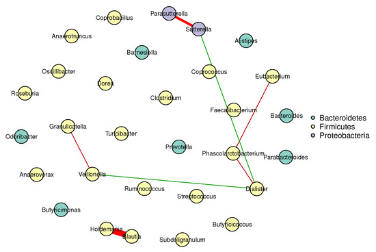
Figure 1. Conditional correlation network of gut microbiota in the lean group (BMI $<25$). Nodes represent 30 retained bacterial genera. Edges denote stable associations (bootstrap frequency $\ge 50\%$): green lines indicate positive correlations, red lines indicate negative correlations, and darker colors represent stronger associations.

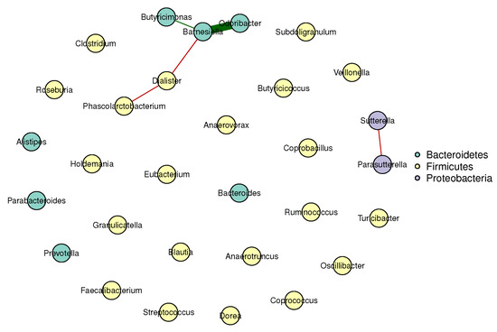
Figure 2. Conditional correlation network of gut microbiota in the obese group (BMI $\ge 25$). Nodes represent 30 retained bacterial genera. Edges denote stable associations (bootstrap frequency $\ge 50\%$): green lines indicate positive correlations, red lines indicate negative correlations, and darker colors represent stronger associations.

Biological Implications of Network Differences

Our analysis reveals meaningful differences between the gut microbial networks of lean and obese individuals, which align with and extend prior findings in gut microbiome research:

• Predominant competitive conditional interactions: Both groups exhibit more negative than positive correlations between bacterial genera (lean group: 71.4% negative correlations; obese group: 60.0% negative correlations). This result is consistent with the findings of Cao et al. [17], Wang et al. [21], Zhang et al. [20] and Coyte et al. [22], and supports the notion that gut microbial interactions are primarily competitive.
• Reduced network complexity in obesity: The obese group had fewer stable edges (five, compared to seven in the lean group) and a lower mean edge strength (0.25, compared to 0.32 in the lean group). These observations indicate weakened conditional associations between bacterial genera in obese individuals, suggesting a decline in gut microbial network complexity.
• Network stability: The lean group’s network had a higher stability score (0.72, compared to 0.58 in the obese group), confirming more reproducible conditional associations and reflecting a robust gut microbial structure. In contrast, the lower stability of the obese group’s network suggested greater inter-individual variability in microbial interactions, a well-documented hallmark of obesity-related gut dysbiosis. This finding also aligned with prior reports of reduced modularity in obese gut microbial networks (Greenblum et al. [23]).

These results validate our multivariate method’s ability to capture biologically meaningful microbial interactions, highlighting competitive balance and core taxa preservation as key to gut health.

5. Conclusions

This paper proposes a two-stage procedure for covariate-adjusted precision matrix estimation in high dimensions. The error vector only requires a bounded lower polynomial moment condition, which is a weaker assumption than the sub-Gaussian conditions of existing methods. We establish non-asymptotic probabilistic upper bounds for the coefficient estimator $\widehat{\mathbf{\Gamma }}$ and precision matrix estimator $\widehat{\mathbf{\Omega }}$ under multiple matrix norms. Despite relaxed assumptions, both estimators achieve optimal convergence rates matching those from stronger sub-Gaussian frameworks. Numerical simulations confirm the method outperforms covariate-unadjusted approaches (Cai et al. [6], Friedman et al. [15]). In a gut microbiome analysis, it successfully captures meaningful microbial network differences between lean and obese groups. Future work may extend this approach to other low moment condition pilot estimators (Avella-Medina et al. [8]).

References

- Wold, S.; Sjostrom, M.; Eriksson, L. PLS-regression: A basic tool of chemometrics. Chemom. Intell. Lab. Syst. 2001, 58, 109–130. [Google Scholar] [CrossRef]
- Harrison, L.; Penny, W.; Friston, K. Multivariate autoregressive modeling of fMRI time series. NeuroImage 2003, 19, 1477–1491. [Google Scholar] [CrossRef]
- Meng, C.; Kuster, B.; Culhane, A.C.; Gholami, A.M. A multivariate approach to the integration of multi-omics datasets. BMC Bioinform. 2014, 15, 162. [Google Scholar] [CrossRef]
- Lee, C.F.; Lee, A.C.; Lee, J. Handbook of Quantitative Finance and Risk Management; Springer: Berlin/Heidelberg, Germany, 2010. [Google Scholar]
- Liu, R.; Yu, G. Estimation of the Error Structure in Multivariate Response Linear Regression Models. WIREs Comput. Stat. 2025, 17, e70021. [Google Scholar] [CrossRef]
- Cai, T.; Liu, W.; Luo, X. A Constrained l1 Minimization Approach to Sparse Precision Matrix Estimation. J. Am. Stat. Assoc. 2011, 106, 594–607. [Google Scholar] [CrossRef]
- Cai, T.T.; Liu, W.; Zhou, H.H. Estimating sparse precision matrix: Optimal rates of convergence and adaptive estimation. Ann. Stat. 2016, 44, 455–488. [Google Scholar] [CrossRef]
- Avella-Medina, M.; Battey, H.S.; Fan, J.; Li, Q. Robust estimation of high-dimensional covariance and precision matrices. Biometrika 2018, 105, 271–284. [Google Scholar] [CrossRef] [PubMed]
- Cai, T.T.; Li, H.; Liu, W.; Xie, J. Covariate-adjusted precision matrix estimation with an application in genetical genomics. Biometrika 2012, 100, 139–156. [Google Scholar] [CrossRef]
- Chen, M.; Ren, Z.; Zhao, H.; Zhou, H. Asymptotically Normal and Efficient Estimation of Covariate-Adjusted Gaussian Graphical Model. J. Am. Stat. Assoc. 2016, 111, 394–406. [Google Scholar] [CrossRef]
- Tan, K.; Romon, G.; Bellec, P.C. Noise covariance estimation in multi-task high-dimensional linear models. Bernoulli 2024, 30, 1695–1722. [Google Scholar] [CrossRef]
- Bickel, P.J.; Levina, E. Covariance regularization by thresholding. Ann. Stat. 2008, 36, 2577–2604. [Google Scholar] [CrossRef] [PubMed]
- Tibshirani, R. Regression Shrinkage and Selection via The Lasso: A Retrospective. J. R. Stat. Soc. Ser. B Stat. Methodol. 2011, 73, 273–282. [Google Scholar] [CrossRef]
- Candes, E.; Tao, T. The Dantzig selector: Statistical estimation when p is much larger than n. Ann. Stat. 2007, 35, 2313–2351. [Google Scholar] [CrossRef] [PubMed]
- Friedman, J.; Hastie, T.; Tibshirani, R. Sparse Inverse Covariance Estimation with the Graphical Lasso. Biostatistics 2008, 9, 432–441. [Google Scholar] [CrossRef]
- Wu, G.D.; Chen, J.; Hoffmann, C.; Bittinger, K.; Chen, Y.Y.; Keilbaugh, S.A.; Bewtra, M.; Knights, D.; Walters, W.A.; Knight, R.; et al. Linking Long-Term Dietary Patterns with Gut Microbial Enterotypes. Science 2011, 334, 105–108. [Google Scholar] [CrossRef]
- Cao, Y.; Lin, W.; Li, H. Large Covariance Estimation for Compositional Data Via Composition-Adjusted Thresholding. J. Am. Stat. Assoc. 2019, 114, 759–772. [Google Scholar] [CrossRef]
- He, Y.; Liu, P.; Zhang, X.; Zhou, W. Robust covariance estimation for high-dimensional compositional data with application to microbial communities analysis. Stat. Med. 2021, 40, 3499–3515. [Google Scholar] [CrossRef]
- Li, D.; Srinivasan, A.; Chen, Q.; Xue, L. Robust Covariance Matrix Estimation for High-Dimensional Compositional Data with Application to Sales Data Analysis. J. Bus. Econ. Stat. 2023, 41, 1090–1100. [Google Scholar] [CrossRef]
- Zhang, S.; Wang, H.; Lin, W. CARE: Large Precision Matrix Estimation for Compositional Data. J. Am. Stat. Assoc. 2025, 120, 305–317. [Google Scholar] [CrossRef]
- Wang, J.; Liang, W.; Li, L.; Wu, Y.; Ma, X. A new robust covariance matrix estimation for high-dimensional microbiome data. Aust. N. Z. J. Stat. 2024, 66, 281–295. [Google Scholar] [CrossRef]
- Coyte, K.Z.; Schluter, J.; Foster, K.R. The ecology of the microbiome: Networks, competition, and stability. Science 2015, 350, 663–666. [Google Scholar] [CrossRef]
- Greenblum, S.; Turnbaugh, P.J.; Borenstein, E. Metagenomic systems biology of the human gut microbiome reveals topological shifts associated with obesity and inflammatory bowel disease. Proc. Natl. Acad. Sci. USA 2012, 109, 594–599. [Google Scholar] [CrossRef]
- Massart, P. Concentration Inequalities and Model Selection; Lecture Notes in Mathematics; Springer: Berlin/Heidelberg, Germany, 2007; Volume 1896, pp. xiv+337. [Google Scholar]
Disclaimer/Publisher’s Note: The statements, opinions and data contained in all publications are solely those of the individual author(s) and contributor(s) and not of MDPI and/or the editor(s). MDPI and/or the editor(s) disclaim responsibility for any injury to people or property resulting from any ideas, methods, instructions or products referred to in the content. |
© 2025 by the author. Licensee MDPI, Basel, Switzerland. This article is an open access article distributed under the terms and conditions of the Creative Commons Attribution (CC BY) license (https://creativecommons.org/licenses/by/4.0/).