A New 5D Chaotic Supply Chain System with Transport Lag: Modeling, Bifurcation Analysis, Offset Boosting Control and Synchronization

Abstract

This paper introduces an enhanced five-dimensional Chaotic Supply Chain Model (5DCSCM) by incorporating a transport lag variable into a previously established four-dimensional model. The newly added differential equation in the transit dynamics of the supply chain model captures the inherent lag between customer demand and the physical response in transportation, modeled as a first-order transport lag system. Through comprehensive numerical simulations, the influence of various system parameters—including customer demand rate, delivery efficiency, information distortion, contingency reserve, safety stock, and transportation lag—are examined. The study utilizes bifurcation diagrams and a Lyapunov Exponent (LE) to investigate tran-sitions between periodic and chaotic behavior. Additionally, the model is extended with offset boosting control, allowing for controlled amplitude adjustment without altering the underlying chaotic dynamics. Offset boosting control (OBC) is useful in chaotic supply chain systems because it stabilizes inventory and order fluctuations by counter-acting the amplification of small disturbances, reducing the bullwhip effect, and im-proving overall system reliability and responsiveness. As an application, integral sliding mode control (ISMC) technique has been applied to achieve complete synchronization between a pair of the 5DCSCM. Synchronization based on ISMC is useful in chaotic supply chain systems because it ensures robust coordination between different tiers, suppresses chaos-induced fluctuations, and maintains stable inventory and order patterns even under disturbances and uncertainties.

1. Introduction

A well-functioning supply chain is a critical backbone of any national economy. It ensures the smooth flow of raw materials, components, and finished goods across various sectors—from agriculture and manufacturing to retail and services [1,2]. Efficient supply chain operations reduce production costs, minimize transport lags, and improve product availability, which in turn enhances consumer satisfaction and business competitiveness [3,4]. In highly globalized markets, countries that can maintain agile and resilient supply chains gain a strategic advantage, attracting foreign investment and enabling seamless participation in international trade networks [5,6]. Moreover, supply chains are essential for maintaining economic stability and responding effectively to crises [7]. Disruptions in logistics, such as those caused by pandemics, natural disasters, or geopolitical tensions, can ripple through an entire economy, leading to inflation, product shortages, and unemployment [8]. Governments and businesses that invest in advanced supply chain management technologies, infrastructure, and analytics can better anticipate risks, ensure national food and energy security, and support long-term sustainable development. As such, strengthening supply chains is not just a matter of operational efficiency, but also a vital element of economic resilience and growth [9].

Transport lag is a critical factor in supply chain management because it directly affects the timing, efficiency, and reliability of product delivery [10]. In practical logistics operations of the supply chain management systems, goods do not move instantaneously between locations—there are inevitable lags caused by transportation distance, traffic congestion, customs processing, weather conditions, or limited carrier capacity [11]. Such lags introduce time gaps between order placement and product receipt, potentially disrupting inventory balance, misaligning supply with demand, and diminishing service quality. If transport lags are not properly modeled or anticipated, firms may experience stockouts, overstocking, elevated holding costs, or the bullwhip effect—where minor variations in demand amplify across the supply chain [12]. Consequently, integrating transport lag into mathematical and simulation-based models is essential for developing realistic, resilient, and adaptive supply chain systems capable of handling uncertainty while maintaining operational continuity.

Chaotic systems are applied in supply chain modeling to capture the inherent nonlinearities, sensitivity to initial conditions, and complex interactions between different supply chain entities [13]. In real-world supply chains, small changes in parameters—such as customer demand, lead times, or information flow—can lead to disproportionately large and unpredictable outcomes, a hallmark of chaos theory [14]. By using chaotic system models, researchers and practitioners can better understand the emergence of irregular fluctuations in inventory levels, order quantities, and production rates. These models help reveal critical thresholds where the system transitions between stable, periodic, and chaotic behavior. Such insights are valuable for designing more resilient supply chains, optimizing control strategies, and preventing disruptive phenomena like the bullwhip effect [15]. Therefore, chaos-based modeling serves not only as a theoretical framework but also as a practical tool for analyzing and managing the dynamic complexity of modern supply chains.

Research on supply chain systems has evolved significantly over the past decades, employing a wide range of approaches to model instability, lags, and nonlinear behavior in global distribution networks. Lu et al. [16] investigated the causes of the bullwhip effect in supply chain management—including oscillation, amplification, and phase lag using system dynamics and the Beer Game model. Jin et al. [17] analyzed how dynamic pricing and demand variability contribute to nonlinear and chaotic patterns in supply chain orders. Han and Wang [18] investigated the chaotic behavior of nonlinear inventory systems using control theory, nonlinear system theory, and chaos theory, and to compare how different supply chain strategies. Makui and Madadi [19] proposed a new method for measuring the bullwhip effect in supply chains using the LE, and to derive insights into its behavior through mathematical analysis. Yan et al. [20] analyzed a supply chain system incorporating computer-aided digital manufacturing processes, investigate its chaotic behavior, and design controllers to stabilize and synchronize the system based on Lyapunov stability theory.

Synchronization of chaotic systems has many applications in secure communication devices [21,22]. Many control methods have been deployed in the control literature for the control and synchronization of chaotic systems such as backstepping control [23], LMI approach [24], sliding mode control [25,26,27,28,29]. Integral sliding mode control (ISMC) is widely used for controlling chaotic systems due to its robustness against system uncertainties and external disturbances. In chaotic systems, small changes in initial conditions can lead to vastly different outcomes, making them highly sensitive and difficult to stabilize. ISMC addresses this challenge by designing a sliding surface from the initial time, ensuring that the system trajectories remain on the sliding manifold throughout the control process. This approach eliminates the reaching phase problem common in traditional sliding mode control, thereby enhancing stability and accuracy. In this research work, we apply the ISMC technique to achieve complete synchronization between a pair of new 5-D chaotic supply chain systems taken as leader and follower systems. ISMC incorporates an integral term into the sliding surface in the control addition, which helps to enhance robustness and removes the reaching phase inherent in the standard sliding mode control (SMC) design [26]. ISMC is a powerful control design, which is useful in many engineering applications [27,28].

The main contribution and novelty of this paper are listed as follows:

(a)

The paper extends an existing 4D Chaotic Supply Chain Model (4DCSCM) by incorporating a transport lag variable as a fifth state, capturing the real-world lag between customer demand and delivery response. This makes the model more representative of actual logistics systems.

(b)

The study provides a comprehensive dynamical analysis of the proposed 5D system using bifurcation diagrams and LE spectra, demonstrating rich behavior including transitions between periodic, chaotic, and equilibrium states under various parameter conditions.

(c)

The study details the control design using ISMC for the complete synchronization of the 5D Chaotic Supply Chain Model (5DCSCM) taken as the leader and follower systems.

This paper is organized as follows. Section 1 introduces the importance of supply chain modeling, emphasizing the role of transport lag and the application of chaotic systems in capturing complex and nonlinear logistics behavior. Section 2 presents the formulation of a 5DCSCM, extending a previously established 4DCSCM framework by incorporating a transport lag variable to reflect realistic logistics dynamics. Section 3 analyzes the system’s dynamic behavior, investigating how variations in key parameters—such as customer demand rate, delivery efficiency, contingency reserve, information distortion, safety stock, and transport lag—affect the stability and chaotic properties of the system. Section 4 introduces an offset boosting control strategy that enables amplitude modulation of chaotic attractors without altering the underlying dynamics. Section 5 presents control results for the synchronization of a pair of 5DCSCM systems taken as leader and follower systems. Section 6 concludes the paper by summarizing the main contributions and discussing the theoretical and practical implications of the proposed model for the design of adaptive, robust, and intelligent supply chain systems.

2. Model of a New 5D Supply Chain Model with Transport Lag

Modeling supply chains with transport lag is critically important in dynamical systems because transport lags inherently influence the stability, responsiveness, and overall behavior of the supply network. Transport lags, which occur due to the time it takes for goods to move between locations, can introduce oscillations, amplifications, or even chaotic dynamics in inventory levels and order rates. By explicitly incorporating the transport lags into mathematical models, researchers and practitioners can better understand the time-dependent interactions between production, inventory, and demand, enabling them to predict system responses under various scenarios. This modeling approach supports the development of more robust control strategies to mitigate risks such as the bullwhip effect, stockouts, and excessive inventory, ultimately leading to more efficient and resilient supply chain operations.

In 2022, Xu et al. [29] proposed a four-tier integrated chaotic supply chain model using a system of four-dimensional differential equations.

$$\left\{\begin{array}{l}{\dot{\mathrm{ɤ}}}_1=-({\mathrm{ɤ}}_2+p{\mathrm{ɤ}}_1)\\ {\dot{\mathrm{ɤ}}}_2=q{\mathrm{ɤ}}_3-(p+1){\mathrm{ɤ}}_2+r{\mathrm{ɤ}}_1\\ {\dot{\mathrm{ɤ}}}_3=s{\mathrm{ɤ}}_2-{\mathrm{ɤ}}_3-{\mathrm{ɤ}}_2{\mathrm{ɤ}}_4\\ {\dot{\mathrm{ɤ}}}_4={\mathrm{ɤ}}_2{\mathrm{ɤ}}_3-(1-\tau ){\mathrm{ɤ}}_4\end{array}\right.$$

(1)

The state variables represent the customer’s actual demand, the retailer’s order quantity, the distributor’s inventory level, and the manufacturer’s production output. The system parameters include

• r: contingency reserve coefficient;
• q: distributor’s delivery efficiency;
• p: customer demand rate;
• s: information distortion rate;
• τ: safety stock coefficient.

When $p=0.2, q=3.5, r=1.5, s=26$, and $\tau =0.3,$ Xu et al. (2022) [29] found a chaotic attractor exhibited by the 4DCSCM (1) for the initial values ${\mathrm{ɤ}}_0=(0.02,0.02,0.02,0.02).$ In fact, for $T=1E4$ s, the Lyapunov exponents (LE) for the Xu system (1) were found to be

$$L{E}_1=0.1730, L{E}_2=0, L{E}_3=-0.5006, L{E}_4=-2.7728$$

(2)

In the 4DCSCM proposed by Xu et al. (2022) [29], the system (1) captures the dynamics between actual customer demand, retailer order quantity, distributor inventory, and manufacturer production rate. However, the model does not account for transport lags, which are a natural and critical part of real-world supply chain operations.

To address this, we introduce an additional state variable to represent the transport lag (${\mathrm{ɤ}}_5$), thereby extending the model into a 5D system. The modified system is governed by the following 5-D dynamics:

$$\left\{\begin{array}{l}{\dot{\mathrm{ɤ}}}_1=-({\mathrm{ɤ}}_2+p{\mathrm{ɤ}}_1)-u{\mathrm{ɤ}}_5\\ {\dot{\mathrm{ɤ}}}_2=q{\mathrm{ɤ}}_3-(p+1){\mathrm{ɤ}}_2+r{\mathrm{ɤ}}_1\\ {\dot{\mathrm{ɤ}}}_3=s{\mathrm{ɤ}}_2-{\mathrm{ɤ}}_3-{\mathrm{ɤ}}_2{\mathrm{ɤ}}_4\\ {\dot{\mathrm{ɤ}}}_4={\mathrm{ɤ}}_2{\mathrm{ɤ}}_3-(1-\tau ){\mathrm{ɤ}}_4\\ {\dot{\mathrm{ɤ}}}_5={\mathrm{ɤ}}_1-{\mathrm{ɤ}}_5\end{array}\right.$$

(3)

In Equation (3), u is transportation lag impact coefficient. ${\mathrm{ɤ}}_1,$ ${\mathrm{ɤ}}_2,$ ${\mathrm{ɤ}}_3,$ ${\mathrm{ɤ}}_4,$ and ${\mathrm{ɤ}}_5$ are state variables in the 5DCSCM (3).

The inclusion of this variable ${\mathrm{ɤ}}_5$ in the 5DCSCM (3) is essential because transportation in supply chains does not occur instantaneously. There is always a time gap between when a product is ordered or demanded (${\mathrm{ɤ}}_1$) and when it physically arrives at its destination. This lag impacts inventory planning, production scheduling, and customer satisfaction. Without considering this factor, models may misrepresent system dynamics, resulting in inaccurate forecasts or suboptimal control strategies.

Physically, the equation ${\dot{\mathrm{ɤ}}}_5={\mathrm{ɤ}}_1-{\mathrm{ɤ}}_5$ describes a first-order lag system. It reflects how the transportation response (e.g., goods in transit or being delivered) gradually follows actual demand over time. The variable ${\mathrm{ɤ}}_5$ can be interpreted as a smoothed or lagged version of ${\mathrm{ɤ}}_1$, capturing how transport operations respond to changes in demand with some transport lag. This dynamic is common in logistics systems and plays a crucial role in the emergence of oscillatory or chaotic behavior in supply chains.

The transportation lag impact coefficient $u$ is a critical factor to study the chaos in supply chain model because lags in the transportation process can significantly amplify fluctuations in inventory levels, demand forecasts, and production schedules—phenomena often associated with the bullwhip effect. In chaotic supply chains, where small disruptions can lead to unpredictable and nonlinear behaviors, transportation lags act as time-lagged feedback that can destabilize the entire system. By quantifying and analyzing this coefficient, researchers and practitioners can better understand how transport lags influence the system dynamics, allowing for the development of more robust control strategies to mitigate chaos, improve responsiveness, and enhance overall supply chain resilience.

When the system parameters in (3) take the values as $p=0.2, q=3.5, r=1.5, s=26, u=0.05$, $\tau =0.3$ and ${\mathrm{ɤ}}_0=(0.02,0.02,0.02,0.02,0.02)$, the LE of the N5DCMTD (3) were computed for the time $1\times {10}^4$ seconds using MATLAB version R2024b as $L{E}_1=0.1745,$ $L{E}_2=0,$ $L{E}_3=-0.6931,$ $L{E}_4=-0.8371$ and $L{E}_5=-2.7446$. This calculation pinpoints that the 5DCSCM (3) is chaotic and dissipative.

For the chaotic case, the 5DCSCM (3) has two equilibrium points given by $Z_0=(0,0,0,0,0)$ and $Z_1=(-11.4173,2.8543,5.8718,23.9429,-11.4173)$. The Jacobian matrix of the 5DCSCM (3) at $Z_0$ has the eigen values $-0.7, -0.2547, -0.9318, -10.5671$ and $8.3536.$ This finding shows that the equilibrium point $Z_0$ is a saddle point. Also, the Jacobian matrix of the 5DCSCM (3) at $Z_1$ has the eigen values $-0.4956, -0.9012,$ $-4.6889$ and $0.9929 \pm 3.6083i.$ This finding shows that the equilibrium point $Z_1$ is a saddle focus point. Thus, the 5DCSCM (3) has two unstable equilibrium points $Z_0$ and $Z_1$. Stability in a supply chain plays a crucial role in maintaining consistent operations, reducing costs, and ensuring customer satisfaction. When a supply chain is stable, it can effectively absorb fluctuations in demand, supply, and lead times without causing large disruptions or oscillations in inventory levels and production schedules. Conversely, instability—often caused by transport lags, poor coordination, or distorted information—can lead to phenomena such as the bullwhip effect, stockouts, overstocking, and ultimately chaotic behavior. These instabilities increase operational costs, reduce service levels, and can compromise the long-term viability of the supply chain. Therefore, analyzing and enhancing supply chain stability is essential for improving resilience, efficiency, and responsiveness in dynamic and uncertain environments.

3. Analysis of System Dynamics

This section explores the qualitative properties of the 5-D chaotic supply chain system (3). The focus is on understanding how changes in parameters and initial values affect the system’s overall performance and response over time. To carry out this investigation, several analytical methods are employed, including LE spectra, bifurcation analysis, and phase space visualization. These tools provide a detailed understanding of the system’s behavior under various conditions, highlighting its complex and evolving nature [30,31].

Chaotic behavior in supply chain systems implies high sensitivity to small changes in demand, lead times, or decision rules. For managers, this means forecasting becomes unreliable, safety stock must be higher, and logistics costs increase due to sudden swings in inventory and transportation needs. When supply chain systems exhibit chaotic behavior, decision-making shifts towards resilience and flexibility, emphasizing real-time monitoring, adaptive ordering policies, and robust control strategies to prevent disruptions. Periodic behavior in supply chain systems provides predictable cycles of inventory and order flows, making it easier for managers to plan production schedules, allocate resources, and optimize logistics operations. In the supply chain models, managers facing chaotic dynamics must prioritize stability, adaptability, and risk management, whereas in periodic regimes, they can focus on efficiency, cost minimization, and long-term planning.

3.1. Effect of Customer Demand Rate

This section focuses on how variations in the parameter $p$ influence the dynamic behavior of the system. Specifically, the parameter $p$ is varied over the interval [0, 0.2], and its effects are examined using bifurcation diagrams and LE spectra, as shown in Figure 1a,b. The findings demonstrate that the system described by 5DCSCM (3) can exhibit both periodic and chaotic dynamics depending on the value of $p$. As shown in Figure 1a, the system demonstrates periodic behavior when the parameter p lies within the interval [0, 0.06]. This periodic nature is supported by the MLE, which remains at zero across this range, as illustrated in Figure 1b. A specific example of this periodicity, corresponding to p = 0.02, is depicted in Figure 1c. In contrast, when the parameter p increases from 0.06 to 0.2, the system undergoes a shift into a chaotic state. This transition is evident in Figure 1a and further confirmed by the emergence of a positive MLE throughout this interval, as presented in Figure 1b. To illustrate the chaotic dynamics, Figure 1d shows the system’s attractor at p = 0.16.

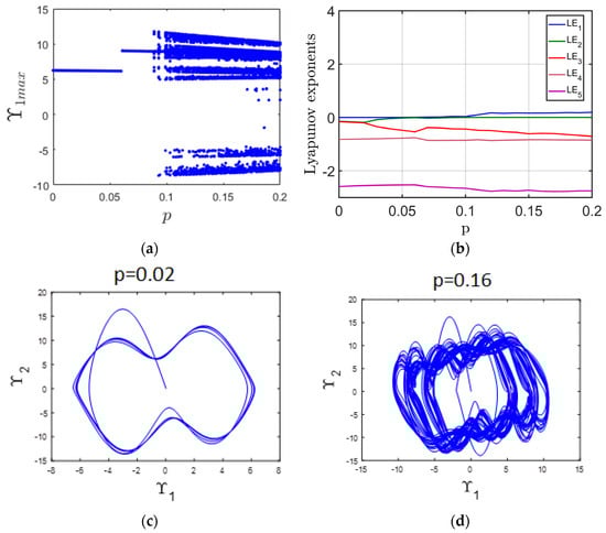
Figure 1. (a) Bifurcation diagram illustrating the system’s response as the parameter p varies; (b) Corresponding LE; (c) ${\mathrm{ɤ}}_1-{\mathrm{ɤ}}_2$ periodic attractor observed at p = 0.02; (d) ${\mathrm{ɤ}}_1-{\mathrm{ɤ}}_2$ chaotic attractor observed at p = 0.16.

If the demand rate (p) is low or stable, the supply chain may exhibit periodic or steady behavior, allowing inventory, orders, and production to adjust smoothly. However, as the customer demand rate increases or becomes more variable, it can push the system into nonlinear and chaotic regimes, particularly when coupled with transportation lags. When transport lag is added as a state-dependent variable, it introduces time-lagged feedback into the system. The transport lag can amplify the effects of fluctuating demand, leading to oscillations, loss of synchronization, and even chaotic behavior in inventory levels and ordering patterns. Essentially, the combination of high or varying customer demand and transport lag reduces the supply chain’s ability to respond promptly and accurately, thereby increasing instability, costs, and the risk of supply-demand mismatches.

3.2. Effect of Distributor’s Delivery Efficiency

This part of the analysis investigates how changes in the parameter q, ranging from 0.5 to 7.5, influence the system’s dynamic behavior. The investigation utilizes both the bifurcation diagram and LE spectrum, as shown in Figure 2a,b. In the ranges [0.5, 1.2] and [1.5, 2.5], the system exhibits periodic motion, evidenced by the zero value of the MLE in Figure 2b. A specific example is illustrated in Figure 2c, where a periodic attractor is observed at q = 2. On the other hand, when q falls within the intervals [1.2, 1.5] and [2.5, 7.5], the system shifts to chaotic dynamics. This transition is reflected in the complex structures of the bifurcation diagram in Figure 2a, and it is further supported by the appearance of a positive MLE in Figure 2b. To illustrate this chaotic state, Figure 2d displays the attractor at q = 4.

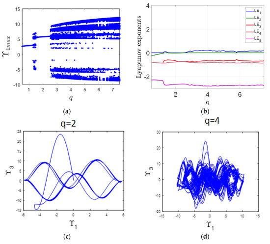
Figure 2. (a) Bifurcation diagram illustrating the system’s response as the parameter q varies; (b) Corresponding LE spectrum; (c) ${\mathrm{ɤ}}_1-{\mathrm{ɤ}}_3$ periodic attractor observed at q = 2; (d) ${\mathrm{ɤ}}_1-{\mathrm{ɤ}}_3$ chaotic attractor observed at q = 4.

The distributor’s delivery efficiency (q) plays a vital role in determining the stability and responsiveness of a supply chain, especially in the presence of transportation lag. When delivery efficiency is high, the distributor can quickly respond to orders, minimizing the impact of transport lags and helping the system maintain periodic or stable behavior. However, if delivery efficiency decreases, even small transportation lags can be magnified, leading to misalignment between supply and demand. This can cause oscillations in inventory and order quantities, eventually driving the system into chaotic behavior. In chaotic conditions, low delivery efficiency exacerbates uncertainty, disrupts the flow of goods and information, and undermines the reliability of the entire supply chain. Therefore, improving delivery efficiency is essential to buffer the negative effects of transportation lags and to maintain orderly, predictable system dynamics.

3.3. Effect Contingency Reserve Coefficient

This subsection analyzes the impact of varying the parameter r within the range of 1 to 3 on the system’s dynamic behavior. The investigation utilizes the bifurcation diagram in Figure 3a alongside the LE spectrum depicted in Figure 3b. When r falls between 1 and 1.9, the system displays chaotic dynamics, as indicated by the complex structures in the bifurcation diagram. This chaotic nature is further confirmed by the presence of a positive MLE in Figure 3b. An example of such chaotic behavior is illustrated in Figure 3c for r = 1.4. In contrast, for r values between 1.9 and 3, the system transitions to a periodic regime. This shift is evident from the bifurcation diagram and is corroborated by the MLE dropping to zero, as shown in Figure 3b. Figure 3d provides an example of this periodic behavior at r = 2.8.

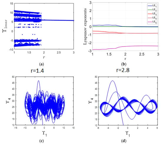
Figure 3. (a) Bifurcation diagram illustrating the system’s response as the parameter r varies; (b) Corresponding LE spectrum; (c) ${\mathrm{ɤ}}_1-{\mathrm{ɤ}}_4$ chaotic attractor observed at r = 1.4; (d) ${\mathrm{ɤ}}_1-{\mathrm{ɤ}}_4$ periodic attractor observed at r = 2.8.

The contingency reserve coefficient represents the buffer or extra capacity maintained to handle uncertainties in a supply chain, and it becomes especially critical in the presence of transportation lags. In a periodic supply chain, an appropriately sized reserve can smooth out fluctuations caused by delays, ensuring consistent fulfillment and avoiding stockouts or overreactions in ordering. However, in chaotic conditions, where small disturbances lead to unpredictable outcomes, the role of the contingency reserve becomes even more significant. If the reserve is too small, the system may become highly sensitive to transport lags, leading to inventory instability and erratic order patterns. Conversely, an overly large reserve might cause overstocking and increased holding costs. Thus, optimizing the contingency reserve coefficient is essential for balancing responsiveness and cost-efficiency, helping to stabilize the supply chain even under chaotic and lag-affected scenarios.

3.4. Effect of Information Distortion Rate

This section examines the influence of varying the parameter s within the range of 16 to 26 on the system’s dynamic behavior. The bifurcation diagram in Figure 4a and the LE spectrum in Figure 4b serve as primary tools for this analysis. When s is between 16 and 18.8, the system demonstrates periodic dynamics, which is reflected by a zero value of the MLE in Figure 4b. An example of this regular behavior is depicted in Figure 4c, showing the periodic attractor at s = 17.

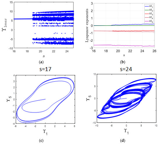
Figure 4. (a) Bifurcation diagram illustrating the system’s response as the parameter s varies; (b) Corresponding LE spectrum; (c) ${\mathrm{ɤ}}_1-{\mathrm{ɤ}}_5$ periodic attractor observed at s = 17; (d) ${\mathrm{ɤ}}_1-{\mathrm{ɤ}}_5$ chaotic attractor observed at s = 24.

In contrast, as s increases from 18.8 to 26, the system undergoes a transition to chaotic dynamics. This change is evident in the bifurcation diagram through the emergence of irregular structures and is further supported by the appearance of a positive MLE in Figure 4b. To illustrate this chaotic behavior, Figure 4d displays the attractor at s = 24. Top of Form Bottom of Form

The information distortion rate (s) reflects the degree to which demand or inventory data becomes inaccurate as it moves through the supply chain, and its impact is significantly amplified when combined with transportation lag. In a periodic system, even moderate distortions can induce significant decision misalignments, including overordering or underordering, particularly when informational feedback is lagged relative to actual system states due to transport lags. This can disrupt the regular cycle and initiate oscillations. In a chaotic supply chain, high information distortion acts as a destabilizing force, magnifying the effects of transport lag and demand variability, which can lead to unpredictable, nonlinear behaviors across different supply chain stages. The combination of distorted data and feedback using transport lag results in poor forecasting, exaggerated bullwhip effects, and overall system inefficiency. Therefore, minimizing information distortion is crucial for maintaining supply chain stability, particularly in supply chain environments prone to chaos and transport lags.

3.5. Effect of Transportation Lag Impact Coefficient

This subsection examines the impact of varying the parameter u within the interval [0, 8] on the system’s dynamic behavior. The analysis is carried out using both the bifurcation diagram and the LE spectrum, as presented in Figure 5a,b, respectively. For values of u between 0 and 6, the system displays chaotic behavior, which is confirmed by the presence of a positive MLE in Figure 5b. A representative chaotic attractor corresponding to u = 2 is illustrated in Figure 5c. In contrast, as u increases from 6 to 8, the system transitions into a stable equilibrium state. This shift is clearly observed in the bifurcation diagram in Figure 5a and is validated by the appearance of a negative MLE in Figure 5b. An example of this steady-state behavior is shown in Figure 5d, which depicts a fixed-point attractor at u = 7.

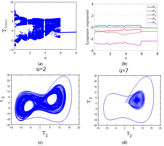
Figure 5. (a) Bifurcation diagram illustrating the system’s response as the parameter u varies; (b) Corresponding LE spectrum; (c) ${\mathrm{ɤ}}_2-{\mathrm{ɤ}}_3$ chaotic attractor observed at u = 2; (d) ${\mathrm{ɤ}}_2-{\mathrm{ɤ}}_3$ point attractor observed at u = 7.

The Transportation Lag Impact Coefficient (u) quantifies the extent to which transport lags influence the dynamics of a supply chain, and its effect becomes critical in both periodic and chaotic regimes. In a periodic supply chain, a low impact coefficient indicates that lags have minimal influence, allowing the system to maintain regular inventory cycles and predictable order flows. However, as the impact coefficient increases, even small transportation lags begin to significantly affect the timing and magnitude of inventory replenishment, causing fluctuations. In a chaotic system, a high transportation lag impact coefficient exacerbates instability, amplifying disruptions and nonlinear behavior across the supply chain. It can lead to severe oscillations, desynchronization between supply and demand, and an overall loss of control. Thus, understanding and managing this coefficient is essential to mitigating the destabilizing effects of transport lags and enhancing the resilience of the supply chain.

3.6. Effect of Safety Stock Coefficient

This subsection investigates the influence of varying the parameter τ within the range [0, 1] on the system’s dynamic behavior. The analysis employs the bifurcation diagram and LE spectrum, presented in Figure 6a,b, respectively. For the values of τ between 0 and 0.98, the system demonstrates chaotic dynamics, as evidenced by the presence of a positive MLE in Figure 6b. A representative chaotic attractor at τ = 0.7 is illustrated in Figure 6c. However, when τ increases to the range [0.98, 1], the system transitions to a stable equilibrium. This change is observable in the bifurcation diagram (Figure 6a) and supported by the negative MLE values shown in Figure 6b. An example of this stable behavior is displayed in Figure 6d, which shows a point attractor at τ = 1.

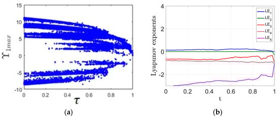
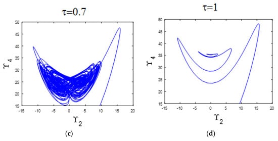
Figure 6. (a) Bifurcation diagram illustrating the system’s response as the parameter $\tau$ varies; (b) Corresponding LE spectrum; (c) ${\mathrm{ɤ}}_2-{\mathrm{ɤ}}_4$ chaotic attractor observed at $\tau$ = 0.7; (d) ${\mathrm{ɤ}}_2-{\mathrm{ɤ}}_4$ point attractor observed at $\tau$= 1.

The safety stock coefficient ($\tau$) determines the level of buffer inventory maintained to protect against demand variability and supply disruptions, and its role becomes increasingly important in the presence of transportation lag. In a periodic supply chain, an appropriately chosen safety stock coefficient helps absorb the impact of transport lags, ensuring smooth order fulfillment and preventing stockouts. However, in a chaotic supply chain, where demand and system responses are highly unpredictable, the effectiveness of safety stock is more complex. If the coefficient is too low, the system becomes vulnerable to disruptions caused by transport lags, leading to frequent shortages and instability. On the other hand, if it is too high, it may result in excessive inventory holding costs and inefficiencies. Therefore, in both periodic and chaotic regimes, the safety stock coefficient must be carefully optimized to balance service levels and costs, especially when transportation lags are significant.

4. Effect of Offset Boosting Control

Offset boosting control (OBC) finds practical justification in chaotic supply chain systems and logistics as it provides an effective control mechanism to regulate the chaotic dynamics that often arises due to nonlinear demand patterns, excessive inventory fluctuations, transport lags, and poor synchronization across multiple tiers of the supply chain, leading to inefficiencies and increased costs. By introducing a tunable offset boosting control parameter, the chaotic supply chain system’s attractor can be shifted into a region of enhanced controllability, thereby reducing volatility and enabling more stable synchronization among suppliers, warehouses, and distributors. In real-world applications, the use of offset boosting control translates into smoother logistics flows, improved inventory balance and reduced operational risks. Thus, the offset boosting control provides a cost-effective means of enhancing both efficiency and resilience in complex chaotic supply chain networks. OBC works by introducing a constant offset to selected state variables, effectively shifting the system’s equilibrium and altering its trajectory in phase space. By doing so, OBC can suppress chaotic oscillations, stabilize the system, and guide it toward a desired periodic or steady-state behavior. In the context of supply chains, applying OBC can reduce unpredictable fluctuations in inventory levels and order rates, thus improving coordination, minimizing the bullwhip effect, and enhancing overall system efficiency and robustness under varying demand or transport lag conditions.

The newly introduced five-dimensional system displays variable-boosting chaotic behavior, allowing for tunable dynamic responses. In particular, the behavior of the system can be intensified by substituting the original variable with a boosted version within the system’s equations, resulting in the following modified form:

$$\left\{\begin{array}{l}{\dot{\mathrm{ɤ}}}_1=-({\mathrm{ɤ}}_2+p{\mathrm{ɤ}}_1)-u({\mathrm{ɤ}}_5+k)\\ {\dot{\mathrm{ɤ}}}_2=q{\mathrm{ɤ}}_3-(p+1){\mathrm{ɤ}}_2+r{\mathrm{ɤ}}_1\\ {\dot{\mathrm{ɤ}}}_3=s{\mathrm{ɤ}}_2-{\mathrm{ɤ}}_3-{\mathrm{ɤ}}_2{\mathrm{ɤ}}_4\\ {\dot{\mathrm{ɤ}}}_4={\mathrm{ɤ}}_2{\mathrm{ɤ}}_3-(1-\tau ){\mathrm{ɤ}}_4\\ {\dot{\mathrm{ɤ}}}_5={\mathrm{ɤ}}_1-({\mathrm{ɤ}}_5+k)\end{array}\right.$$

(4)

In offset boosting control for chaotic supply chain systems, the boosting parameter k represents the strength or magnitude of the corrective action applied to counteract fluctuations in inventory or orders. A higher value of k increases the system (4)’s responsiveness, helping to rapidly reduce deviations from desired inventory or order levels. Too high a value of k can lead to overcompensation in (4), causing oscillations or instability. Too low a value of k makes the control weak, allowing chaotic fluctuations to persist in (4).

The variable-boosting chaotic behavior for the modified system (4) is demonstrated by the ${\mathrm{ɤ}}_2-{\mathrm{ɤ}}_5$ attractors shown in Figure 7a. When the parameter k takes on negative values, the system’s attractors are displaced toward the positive axis, while a positive k causes a shift in the negative direction. This mechanism allows the chaotic signal to be transformed from a bipolar to a unipolar form, as illustrated in Figure 7b. This unique property offers significant potential for applications in secure communication systems and other engineering domains.

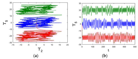
Figure 7. (a) ${\mathrm{ɤ}}_2-{\mathrm{ɤ}}_5$ Chaotic Attractors and (b) ${\mathrm{ɤ}}_5$ for Different Values of Offset Boosting Parameter for Equation (4): k = 0 (blue), k = 20 (red), k = −20 (green).

5. Complete Synchronization of 5-D Chaotic Supply Chain Models

In chaotic supply chain systems, the synchronization of dynamic behavior between different agents—such as suppliers, distributors, and manufacturers—is essential to maintain consistency and prevent systemic disruption. In supply chain systems, decision-makers can employ synchronization methods to align the dynamic behaviors of interconnected subsystems such as suppliers, manufacturers, distributors, and retailers, thereby reducing instability and inefficiencies. Synchronization of chaotic supply chain systems enables the coordination of inventory levels, production schedules, and logistics flows, mitigating the bullwhip effect and ensuring smoother transitions of goods and information across the chain. By applying control-based synchronization for the chaotic supply chain systems, managers can stabilize chaotic fluctuations, achieve consistent demand–supply matching, and improve predictability in lead times and transportation schedules.

Traditional control methods often fall short in managing the sensitivity to initial conditions and unpredictable responses that characterize chaotic systems. The ISMC is particularly well-suited for such applications due to its inherent robustness and capacity to enforce synchronization despite parameter uncertainties and external disturbances. The presence of transport lag further complicates synchronization, introducing additional phase lags that can destabilize system trajectories. ISMC addresses this challenge by eliminating the reaching phase and maintaining the system on the predefined sliding surface from the onset, making it a reliable choice for ensuring consistent coordination in complex, transport lag-influenced supply chains.

This section presents control results for the complete synchronization of 5D chaotic supply chain models (5DCSCM) using ISMC. The ISMC is widely used in synchronization of chaotic systems due to its robustness, precision, and ability to handle uncertainties and external disturbances effectively. In synchronization tasks—especially when dealing with chaotic systems that are highly sensitive to initial conditions—ensuring that the trajectories of a slave system follow those of a master system is challenging. ISMC overcomes this by designing a sliding surface from the initial time, which eliminates the traditional reaching phase and ensures the system states stay on the desired trajectory throughout the process. This feature is particularly important for chaotic synchronization, where even small deviations can lead to desynchronization. Furthermore, ISMC can guarantee finite-time convergence and maintain synchronization performance even in the presence of model mismatches or time-varying parameters, making it a powerful and reliable technique for synchronizing chaotic systems. Figure 8 presents a block diagram for the complete synchronization of the two 5D chaotic supply chain models using ISMC.

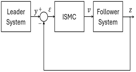
Figure 8. Block diagram for the complete synchronization of 5-D chaotic supply chain models (5) and (6) using ISMC.

As the leader system, we consider the 5DCSCM given as follows:

$$\left\{\begin{array}{l}{\dot{y}}_1=-(y_2+p{y}_1)-u{y}_5\\ {\dot{y}}_2=q{y}_3-(p+1)y_2+r{y}_1\\ {\dot{y}}_3=s{y}_2-y_3-y_2{y}_4\\ {\dot{y}}_4=y_2{y}_3-(1-\tau )y_4\\ {\dot{y}}_5=y_1-y_5\end{array}\right.$$

(5)

As the follower system, we take the 5DCSCM (with feedback controls) given by the following dynamics:

$$\left\{\begin{array}{l}{\dot{z}}_1=-(z_2+p{z}_1)-u{z}_5+v_1\\ {\dot{z}}_2=q{z}_3-(p+1)z_2+r{z}_1+v_2\\ {\dot{z}}_3=s{z}_2-z_3-z_2{z}_4+v_3\\ {\dot{z}}_4=z_2{z}_3-(1-\tau )z_4+v_4\\ {\dot{z}}_5=z_1-z_5+v_5\end{array}\right.$$

(6)

In (6), $v_1,v_2,v_3,v_4,v_5$ are the controls to be designed by using ISMC technique [26].

The synchronization error between the 5DCSCM (5) and (6) is defined as follows:

$${\epsilon }_i=z_i-y_i, (i=1,2,\dots ,5)$$

(7)

The error dynamics can be easily computed as follows:

$$\left\{\begin{array}{l}{\dot{\epsilon }}_1=-p{\epsilon }_1-{\epsilon }_2-u{\epsilon }_5+v_1\\ {\dot{\epsilon }}_2=q{\epsilon }_3-(p+1){\epsilon }_2+r{\epsilon }_1+v_2\\ {\dot{\epsilon }}_3=s{\epsilon }_2-{\epsilon }_3-z_2{z}_4+y_2{y}_4+v_3\\ {\dot{\epsilon }}_4=z_2{z}_3-y_2{y}_3-(1-\tau ){\epsilon }_4+v_4\\ {\dot{\epsilon }}_5={\epsilon }_1-{\epsilon }_5+v_5\end{array}\right.$$

(8)

In the design of ISMC for stabilizing the error dynamics (8), an integral sliding surface is assigned for every error variable ${\epsilon }_i,$ $(i=1,\dots ,5)$ as follows:

$$s_i={\epsilon }_i+{\alpha }_i{\displaystyle \underset{0}{\overset{t}{\int }}{\epsilon }_i(\omega )d\omega }, (i=1,2,\dots ,5)$$

(9)

Taking the time-derivative of the integral sliding surfaces, we obtain the following:

$${\dot{s}}_i={\dot{\epsilon }}_i+{\alpha }_i{\epsilon }_i, (i=1,2,\dots ,5)$$

(10)

We define the ISMC by the following equations:

$$\left\{\begin{array}{l}{v}_1=p{\epsilon }_1+{\epsilon }_2+u{\epsilon }_5-{\alpha }_1{\epsilon }_1-{\beta }_1\mathrm{sgn}(s_1)-{\gamma }_1{s}_1\\ v_2=-q{\epsilon }_3+(p+1){\epsilon }_2-r{\epsilon }_1-{\alpha }_2{\epsilon }_2-{\beta }_2\mathrm{sgn}(s_2)-{\gamma }_2{s}_2\\ v_3=-s{\epsilon }_2+{\epsilon }_3+z_2{z}_4-y_2{y}_4-{\alpha }_3{\epsilon }_3-{\beta }_3\mathrm{sgn}(s_3)-{\gamma }_3{s}_3\\ v_4=-z_2{z}_3+y_2{y}_3+(1-\tau ){\epsilon }_4-{\alpha }_4{\epsilon }_4-{\beta }_4\mathrm{sgn}(s_4)-{\gamma }_4{s}_4\\ v_5=-{\epsilon }_1+{\epsilon }_5-{\alpha }_5{\epsilon }_5-{\beta }_5\mathrm{sgn}(s_5)-{\gamma }_5{s}_5\end{array}\right.$$

(11)

We remark that the constants ${\alpha }_i,{\beta }_i,{\gamma }_i,$ $(i=1,2,\dots ,5)$ in Equation (11) are all positive.

Substituting (11) into (8), we obtain the closed-loop error dynamics as given below.

$$\left\{\begin{array}{l}{\dot{\epsilon }}_1=-{\alpha }_1{\epsilon }_1-{\beta }_1\mathrm{sgn}(s_1)-{\gamma }_1{s}_1\\ {\dot{\epsilon }}_2=-{\alpha }_2{\epsilon }_2-{\beta }_2\mathrm{sgn}(s_2)-{\gamma }_2{s}_2\\ {\dot{\epsilon }}_3=-{\alpha }_3{\epsilon }_3-{\beta }_3\mathrm{sgn}(s_3)-{\gamma }_3{s}_3\\ {\dot{\epsilon }}_4=-{\alpha }_4{\epsilon }_4-{\beta }_4\mathrm{sgn}(s_4)-{\gamma }_4{s}_4\\ {\dot{\epsilon }}_5=-{\alpha }_5{\epsilon }_5-{\beta }_1\mathrm{sgn}(s_5)-{\gamma }_5{s}_5\end{array}\right.$$

(12)

Next, we state and prove an important ISMC result for the chaos synchronization between the 5DCSCM (5) and (6).

Theorem 1. 

The ISMC defined by Equation (11) globally synchronizes the two 5DCSCM (5) and (6) for all values of their states, where ${\alpha }_i,{\beta }_i,{\gamma }_i,$ $(i=1,2,\dots ,5)$ are positive constants.

Proof. 

This result is proved by means of the Lyapunov stability theory [32].

We define the Lyapunov function by

$$V(s_1,s_2,s_3,s_4,s_5)={\displaystyle \frac{1}{2}}{s}_1^2+{\displaystyle \frac{1}{2}}{s}_2^2+{\displaystyle \frac{1}{2}}{s}_3^2+{\displaystyle \frac{1}{2}}{s}_4^2+{\displaystyle \frac{1}{2}}{s}_5^2$$

(13)

It is easy to check that $V$ is a quadratic and positive definite function on $R^5$.

Using (10) and (12), the time-derivative of the Lyapunov function $V$ is found as

$$\dot{V}=-{\displaystyle \sum _{i=1}^5{\beta }_i}|s_i|-{\displaystyle \sum _{i=1}^5{\alpha }_i}{s}_i^2$$

(14)

From Equation (14), we deduce that $\dot{V}$ is a negative definite function on $R^5$.

Using Lyapunov Stability Theory [32], we conclude that $s_i(t)\to 0$ as $t\to \infty$ for $i=1,\dots ,5$.

Hence it follows that ${\epsilon }_i(t)\to 0$ as $t\to \infty$ for $i=1,\dots ,5$. This completes the proof. ☐

For numerical simulations in MATLAB, we take the constants of the 5-D chaotic supply chain systems (5) and (6) as in the chaotic case, viz.

$${\alpha }_i=10,{\beta }_i=0.5, {\gamma }_i=6,(i=1,2,\dots ,5)$$

(15)

For simulations, we take the ISMC parameters as follows:

$$p=0.2,q=3.5,r=1.5,s=2.6,u=0.05,\tau =0.3$$

(16)

The initial state of the 5-D chaotic supply chain system (5) is taken as

$$y_1(0)=1.2, y_2(0)=6.3, y_3(0)=4.9, y_4(0)=2.8, y_5(0)=6.4$$

(17)

The initial state of the 5DCSCM (6) is taken as

$$z_1(0)=2.7, z_2(0)=0.1, z_3(0)=3.2, z_4(0)=6.1, z_5(0)=1.9$$

(18)

Figure 9 shows the convergence of the synchronization errors ${\epsilon }_i(t)$ to zero as $t\to \infty$ for $i=1,\dots ,5$. This convergence behavior of the synchronization errors in Figure 9 confirms that the ISMC technique effectively achieves complete synchronization between the 5D chaotic supply chain systems despite initial deviations, ensuring robust and stable tracking performance. The quick settling time and absence of overshoot or oscillations further demonstrate the efficiency and stability of the control strategy under potentially chaotic dynamics.

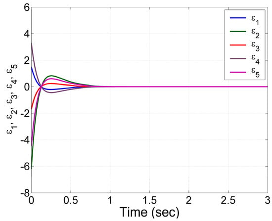
Figure 9. Time-history of the synchronization errors ${\epsilon }_i(t),$ $(i=1,2,\dots ,5)$.

The practical implementation of synchronization in real-world supply chains can be seen in contexts such as automated warehouse coordination, real-time inventory management across multiple locations, and harmonized production scheduling among globally distributed factories. In such cases, chaos synchronization ensures that fluctuations in one node of the supply chain do not cause unpredictable outcomes in another, particularly when transport lags are present. ISMC-based synchronization enables better visibility and control across the supply chain network, making it possible to align the dynamics of suppliers and distributors, optimize replenishment timing, and avoid both understocking and overstocking. These benefits contribute directly to cost reduction, service level improvement, and enhanced supply chain resilience.

6. Conclusions

This study proposed a novel five-dimensional chaotic supply chain model by incorporating a transport lag variable into an existing 4D model by Xu et al. [26], thereby enhancing its realism and relevance to real-world logistics. Through extensive numerical simulations, we analyzed how variations in system parameters affect the dynamics of the supply chain, with a particular focus on transitions between periodic, chaotic, and stable behaviors. The results demonstrate that transport lag plays a critical role in shaping system dynamics and can significantly influence stability and predictability. In future work, we intend to extend the dynamical analysis in our research work on the 5-D chaotic supply chain system by linking the reported metrics—such as Lyapunov exponents, attractor behavior, and equilibrium stability—to operational performance indicators relevant to supply chain practice. These include service-level measures, stockout and overstock probabilities, holding and backorder cost metrics, and the amplitude of the bullwhip effect. Establishing these connections will help translate the underlying system dynamics into actionable managerial insights and improve the practical applicability of the proposed framework.

Additionally, the use of offset boosting control (OBC) provides a mechanism to modulate system outputs without altering the inherent chaotic structure, offering practical potential applications. A detailed justification of the OBC approach using a control criterion consistent with supply chain management (SCM) principles, along with an analysis of trade-offs and appropriate k-ranges to prevent overcompensation, will be included as part of our future work. Finally, we derived new control results using ISMC technique for achieving complete synchronization between a pair of the 5-D chaotic supply chain models taken as the leader and follower systems.

In future work, we also aim to validate the proposed chaotic supply chain framework through empirical studies by mapping system parameters and control performance to operational Key Performance Indicators (KPIs) such as order fulfillment rate, lead time variability, and logistics cost efficiency. This linkage will strengthen the practical applicability of the proposed model in supply chain decision-making and performance evaluation

References

- Ahmad Amouei, M.; Valmohammadi, C.; Fathi, K. Proposing a conceptual model of the sustainable digital supply chain in manufacturing companies: A qualitative approach. J. Enterp. Inf. Manag. 2024, 37, 544–579. [Google Scholar] [CrossRef]
- Tulli, S.K.C. Leveraging Oracle NetSuite to Enhance Supply Chain Optimization in Manufacturing. Int. J. Acta Inform. 2024, 3, 59–75. [Google Scholar]
- Priyadarshini, J.; Singh, R.K.; Mishra, R.; Chaudhuri, A.; Kamble, S. Supply chain resilience and improving sustainability through additive manufacturing implementation: A systematic literature review and framework. Prod. Plan. Control 2025, 36, 309–332. [Google Scholar] [CrossRef]
- Emon, M.M.H.; Khan, T. Unlocking sustainability through supply chain visibility: Insights from the manufacturing sector of Bangladesh. Braz. J. Oper. Prod. Manag. 2024, 21, 2194. [Google Scholar] [CrossRef]
- Rashid, A.; Baloch, N.; Rasheed, R.; Ngah, A.H. Big data analytics-artificial intelligence and sustainable performance through green supply chain practices in manufacturing firms of a developing country. J. Sci. Technol. Policy Manag. 2025, 16, 42–67. [Google Scholar] [CrossRef]
- Al-khatib wael, A.; Khattab, M. How can generative artificial intelligence improve digital supply chain performance in manufacturing firms? Analyzing the mediating role of innovation ambidexterity using hybrid analysis through CB-SEM and PLS-SEM. Technol. Soc. 2024, 78, 102676. [Google Scholar] [CrossRef]
- Hong, L.; Hales, D.N. How blockchain manages supply chain risks: Evidence from Indian manufacturing companies. Int. J. Logist. Manag. 2024, 35, 1604–1627. [Google Scholar] [CrossRef]
- Lee, K.L.; Amin, A.J.; Alzoubi, H.M.; Alshurideh, M.; El Khatib, M.; Joghee, S.; Nair, K. Investigating the factors affecting e-procurement adoption in supply chain performance: An empirical study on Malaysia manufacturing industry. Uncertain Supply Chain Manag. 2024, 12, 615–632. [Google Scholar] [CrossRef]
- Liu, J.; Jiang, P.; Zhang, J. A blockchain-enabled and event-driven tracking framework for SMEs to improve cooperation transparency in manufacturing supply chain. Comput. Ind. Eng. 2024, 191, 110150. [Google Scholar] [CrossRef]
- Azadeh, A.; Atrchin, N.; Salehi, V.; Shojaei, H. Modelling and improvement of supply chain with imprecise transportation delays and resilience factors. Int. J. Logist. Res. Appl. 2014, 17, 269–282. [Google Scholar] [CrossRef]
- Paul, S.K.; Asian, S.; Goh, M.; Torabi, S.A. Managing sudden transportation disruptions in supply chains under delivery delay and quantity loss. Ann. Oper. Res. 2019, 273, 783–814. [Google Scholar] [CrossRef]
- Lajimi, C.; Boufaied, A.; Korbaa, O. Assessing and modelling transport delays risk in supply chains. Int. J. Adv. Oper. Manag. 2017, 9, 225–245. [Google Scholar] [CrossRef]
- Sharma, A. Artificial intelligence for sense making in survival supply chains. Int. J. Prod. Res. 2025, 63, 435–458. [Google Scholar] [CrossRef]
- Stapleton, D.; Hanna, J.B.; Ross, J.R. Enhancing supply chain solutions with the application of chaos theory. Supply Chain Manag. Int. J. 2006, 11, 108–114. [Google Scholar] [CrossRef]
- Lou, W.; Ma, J.; Zhan, X. Bullwhip entropy analysis and chaos control in the supply chain with sales game and consumer returns. Entropy 2017, 19, 64. [Google Scholar] [CrossRef]
- Lu, C. Research on bullwhip effect management in supply chain based on system dynamics. J. Phys. Conf. Ser. 2021, 1910, 012034. [Google Scholar] [CrossRef]
- Jin Lu, Y.; Tang, X.; Zhang, Y. Study on the Chaos of Bullwhip Effect Under Price Fluctuation. J. Syst. Sci. Inf. 2005, 3, 296–302. [Google Scholar]
- Han, W.; Wang, J. The impact of cooperation mechanism on the chaotic behaviours in nonlinear supply chains. Eur. J. Ind. Eng. 2015, 9, 595–612. [Google Scholar] [CrossRef]
- Makui, A.; Madadi, A. The bullwhip effect and Lyapunov exponent. Appl. Math. Comput. 2007, 189, 35–40. [Google Scholar] [CrossRef]
- Yan, L.; Liu, J.; Xu, F.; Teo, K.L.; Lai, M. Control and synchronization of hyperchaos in digital manufacturing supply chain. Appl. Math. Comput. 2021, 391, 125646. [Google Scholar] [CrossRef]
- Tang, R.; Jiang, Z.; Zhang, D.; Wang, J. Dual-channel chaos synchronization in two mutually injected semiconductor ring lasers. Photonics 2025, 12, 348. [Google Scholar] [CrossRef]
- Hadji, M.M.; Ladaci, S. A novel secure communication scheme design using a fractional-order adaptive observer-based synchronization. J. Control Autom. Electr. Syst. 2025, 36, 267–282. [Google Scholar] [CrossRef]
- Peng, X.; Zhang, Z.; Zhang, A.; Yuen, K.-V. Antisaturation backstepping control for quadrotor slung load system with fixed-time prescribed performance. IEEE Trans. Aerosopace Electron. Syst. 2024, 60, 4170–4181. [Google Scholar] [CrossRef]
- Echi, N.; Benabdallah, A. Delay-dependent stabilization of a class of time-delay nonlinear systems: LMI approach. Adv. Differ. Equ. 2017, 271, 271. [Google Scholar] [CrossRef]
- Rasouli, M.; Zare, A.; Hallaji, M.; Alizadehsani, R. The Synchronization of a Class of Time-Delayed Chaotic Systems Using Sliding Mode Control Based on a Fractional-Order Nonlinear PID Sliding Surface and Its Application in Secure Communication. Axioms 2022, 11, 738. [Google Scholar] [CrossRef]
- Vaidyanathan, S.; Lien, C.H. Applications of Sliding Mode Control in Science and Engineering; Springer: New York, NY, USA, 2017. [Google Scholar]
- Wu, X.; Ge, S.; Wang, Y. Distributed adaptive integral sliding mode affine formation control of multi-robot systems with event-triggered mechanism. Phys. Scr. 2025, 100, 075220. [Google Scholar] [CrossRef]
- Wang, Y.; Tang, X.; Jiang, Y.; Li, X.; Zhan, X. Adaptive integral sliding mode control strategy for vehicular platoon with prescribed performance. Sci. Rep. 2025, 15, 14156. [Google Scholar] [CrossRef]
- Xu, X.; Kim, H.-S.; You, S.-S.; Lee, S.-D. Active management stretegy for supply chain system using nonlinear control synthesis. Int. J. Dyn. Control 2022, 10, 1981–1995. [Google Scholar] [CrossRef]
- Sambas, A.; Vaidyanathan, S.; Mamat, M.; Mohamed, M.A.; Sanjaya, W.S.M. A New Chaotic System with a Pear-Shaped Equilibrium and Its Circuit Simulation. Int. J. Electr. Comput. Eng. 2018, 8, 4951–4958. [Google Scholar] [CrossRef]
- Sambas, A.; Vaidyanathan, S.; Mamat, M.; Sanjaya, W.S.M.; Prastio, R.P. Design, analysis of the Genesio-Tesi chaotic system and its electronic experimental implementation. Int. J. Control Theory Appl. 2016, 9, 141–149. [Google Scholar]
- Khalil, H.K. Nonlinear Systems, 3rd ed.; Prentice Hall: Hoboken, NJ, USA, 2002. [Google Scholar]
Disclaimer/Publisher’s Note: The statements, opinions and data contained in all publications are solely those of the individual author(s) and contributor(s) and not of MDPI and/or the editor(s). MDPI and/or the editor(s) disclaim responsibility for any injury to people or property resulting from any ideas, methods, instructions or products referred to in the content. |
© 2025 by the authors. Licensee MDPI, Basel, Switzerland. This article is an open access article distributed under the terms and conditions of the Creative Commons Attribution (CC BY) license (https://creativecommons.org/licenses/by/4.0/).