Modeling Competitive Dynamics Between Healthy and Cancerous Liver Cells with Yes-Associated Protein (YAP) Hyperactivation

Abstract

Current treatments for hepatocellular carcinoma (HCC) include partial hepatectomy (PH), where two-thirds of the liver is removed. However, when some cancer remains after PH, competition for resources and survival occurs between healthy and cancerous cells. Recent studies suggest that hyperactivation of yes-associated protein (YAP) could be a non-invasive treatment option for HCC. In this study, we propose two simple ordinary differential equation models of resource competition in HCC livers after PH, one capturing the natural dynamics of resource competition between healthy and cancer cells and the other incorporating YAP hyperactivation therapy. We perform full qualitative and quantitative analyses of these models and validate them on experimental data. Our numerical simulations reveal that treatment schedules must be prescribed based on a patient’s tumor aggression. We also found that a high dose of treatment is necessary to completely clear a tumor in all patients, leading us to suggest prescribing YAP hyperactivation therapy in lower doses with other treatments for HCC for the best patient outcomes.

1. Introduction

Primary liver cancers are the third-leading cause of cancer-related deaths worldwide [1]. Hepatocellular carcinoma (HCC) makes up nearly 90% of liver cancer cases [2] and is projected to be the second deadliest cancer in American men by 2030 [3]. Risk factors for HCC depend on the region/country of origin of the patient [4] but tend to include chronic Hepatitis B or Hepatitis C infection, cirrhosis, and non-alcoholic fatty liver disease. Other risk factors include alcohol and aflatoxin B1 (AFB1) consumption [4,5,6]. Treatment options for localized and recurrent liver cancer include partial hepatectomy (PH), radiation and ablation, liver transplantation, and immunotherapy [6,7]. Increasingly, there has been a push for cellular [8,9,10,11] and genetic [7,12,13,14] therapies.

Partial hepatectomy (PH) is a well-studied treatment for liver cancers [15,16,17,18], where up to 70% of the liver is cut and removed from an organism. After PH, hepatocytes proliferate to restore the liver to a state where it can fulfill its required metabolic functions [19,20,21]. Although liver regeneration is highly regulated after liver resection [21], underlying liver disease and pressure on hepatocytes to proliferate could lead to abnormal tissue growth and tumor development [20,22,23,24]. Chiche et al. [25] found that more than 40% of non-cirrhotic HCC patients who underwent PH experienced recurrence within 30 months of treatment, and Zhu et al. [26] found that PH induced hepatocellular carcinoma in zebrafish.

Recently, Moya et al. found that tumor cells grow faster if surrounding liver cells do not have YAP (yes-associated protein) [12]. Hyperactivation of YAP in surrounding liver cells caused tumors to shrink to up to an eighth of the tumor size with average YAP activation, leading Moya et al. to suggest YAP activation as a treatment strategy for liver cancer [12]. Due to heterogeneity between tumor cells [8], boosting surrounding tissues may aid the immune system in the fight against tumors of various types [9].

Previous competition models in cancer address the dynamics between tumor cells and the healthy cells around them. However, these models often focus on other types of cancer or lack specificity, diluting their value for the problem at hand. For example, Abernathy et al. [27] construct a competition model for breast cancer, Ch-Chaoui and Mokni [28] model competition between the immune system and tumor, and Gatenby [29] creates a competition model for a generic cancer. Some previous mathematical models specific to HCC account for these dynamics but are more complex, involve many strict assumptions, and do not incorporate gene therapies. Manda and Chirove [30] considered the dynamics between healthy liver cells and HCC under the assumption that the Hepatitis B virus and immune cells contributed to these dynamics. Comparatively, Shen et al. and Shafiekhani et al. focus on immune–cancer interactions [31,32]. Shen et al. [31] incorporated Ter cells, TGF-$\beta$ (a cell growth protein), and serum artemin (a molecule that aids in the growth of neurons), while Shafiekhani et al. [32] included PD-1, PD-L1, and radiation therapy. These studies by Manda and Chirove [30], Shen et al. [31], and Shafiekhani et al. [32] overly rely on specific assumptions and scenarios not relevant to the usage of YAP hyperaction as a therapy for HCC. Others choose to complicate the dynamics of competition between healthy and cancerous liver cells by using partial differential equation (PDE) models: Gatenby and Gawlinski [33], Hillen et al. [34], and Peng et al. [35] consider cancer invading hepatocytes via PDEs with diffusion terms, and Cho and Levy [36] build on these models to also include chemotherapy and target drug therapy. Although these models incorporate spatial heterogeneity, they cannot be interpreted in the context of administering gene therapy. Due to the novelty of YAP hyperactivation and other forms of gene therapy, there is a lack of existing literature incorporating it as a treatment option in mathematical models of HCC.

In this study, we account for YAP activation as an intervention strategy in the context of healthy liver cells and HCC dynamics. We aim to answer the following question: can YAP hyperactivation clear a tumor; if so, what is the minimal treatment profile needed to improve patient outcomes? We propose two simple mathematical models: the first captures the dynamics between healthy and cancerous liver cells, while the second is extended to incorporate these dynamics when YAP is hyperactivated. We describe the new models in Section 2 of this paper. In Section 3, we present the qualitative analysis, parameter estimation, and numerical results for the two models. Lastly, we draw conclusions on our findings and suggests areas of future work in Section 4.

2. Materials and Methods

In this section, we list the biological assumptions and hypotheses underlying our model, develop our model of healthy and cancer cell interaction in the liver, and describe the parameter estimation problems.

2.1. Biological Assumptions

To model the dynamics of the interactions between healthy and cancerous hepatocytes, we use the following set of simplifying assumptions:

• There is a homogeneous mixture of “healthy” (normal) and cancer hepatocytes.
• Hepatocytes start reproducing after hepatectomy or liver damage to reconstruct the liver [20,21,37].
• Healthy and cancerous cells compete for resources and can cause apoptosis in each other [9,23,38,39,40,41].
• Healthy cells have an activated yes-associated protein (YAP) gene, which helps restrict the growth of cancer cells [42]; only hyperactivation of this gene can result in healthy cells clearing cancerous cells [12].
• In the absence of cancer, normal liver cells will grow logistically to the original size of the liver [38].
• The absence of healthy cells corresponds to a dead organism. We assume a marginal number of healthy cells are always present.
• Cancer cells grow logistically to their carrying capacity as the healthy liver cell population approaches zero.
• We take the “healthy” cell compartment to consist primarily of hepatocytes [19,20,21,37] and, to a lesser extent, Kupffer, stellate, and sinusoidal endothelial cells [37,43] since hepatocytes are the drivers of liver regeneration followed by the other types of healthy liver cells.
• No external carcinogenic factors are present; thus, healthy cells cannot produce mutant cancerous cells [44].
• Cancer cells cannot produce healthy cells since reverse mutation is extremely rare [45].
• YAP gene treatment reinforces healthy cells to fight more efficiently against cancer cells [12].

2.2. Mathematical Model

Incorporating the assumptions in Section 2.1, we construct a simple model that describes the dynamics between healthy and cancerous liver cells:

$$\begin{array}{cc}\hfill {\displaystyle \frac{dL}{dt}}& ={\lambda }_L\left(1-{\displaystyle \frac{L+{\gamma }_{C}C}{K_L}}\right)L,L\left(0\right)=L_0\hfill \\ \hfill {\displaystyle \frac{dC}{dt}}& ={\lambda }_C\left(1-{\displaystyle \frac{{\gamma }_{L}L+C}{K_C}}\right)C,C\left(0\right)=C_0.\hfill \end{array}$$

(1)

The state variables, L and C, represent “healthy” and cancerous liver cells, respectively. The healthy compartment consists primarily of hepatocytes and, to a lesser extent, Kupffer, stellate, and sinusoidal endothelial cells [46,47,48], while the cancerous compartment consists only of cancerous cells [49]. Both compartments of cells grow logistically at rates ${\lambda }_L$ (week⁻¹) and ${\lambda }_C$ (week⁻¹), respectively. Healthy cells restrict the growth of cancer at rate ${\gamma }_L$ (dimensionless) but are themselves limited by cancer cells at rate ${\gamma }_C$ (dimensionless). Moya et al. [12] found that tumor cells compete with liver cells such that the population with the higher fitness wins out. In fact, they noted that survival of either population was not absolute but instead relative to the fitness of the other population. Thus, ${\gamma }_L$ and ${\gamma }_C$ correspond to the relative fitness of liver cells and cancer cells. This is called the influence of one population on the other. In the case where there is no tumor present (i.e., $C=0$), the healthy population will grow to its carrying capacity, $K_L$ (mm³). Similarly, if there were no healthy cells present, the cancer population would grow to its carrying capacity, $K_C$ (mm³). Note, however, that the liver is a vital organ and no vertebrates can survive without it, meaning this scenario is equivalent to physical death.

We also impose the conditions

$$K_L<K_C\mathrm{and}{\gamma }_L<1<{\gamma }_C$$

(2)

to account for the increased carrying capacity of the cancerous cells and the increased influence of cancerous cells on the normal liver cell population’s ability to survive. According to [12,50], liver cells are less fit and use fewer resources than cancer cells. This implies that a liver cell is less competitive than a cancer cell, and therefore cancer cells compete more with each other than with liver cells. As such, we must impose ${\gamma }_L<1$. Comparatively, cancer cells are more fit and aggressive in their acquisition of resources than healthy liver cells [12,51,52]. It follows that liver cells compete more with cancer cells than with themselves. So, ${\gamma }_C>1$. We take ${\gamma }_C$ to be a patient-specific quantification of a cancer’s “aggressiveness,” where a larger value of ${\gamma }_C$ corresponds to a more aggressive and resource-hungry tumor.

Note that hyperactivation of the YAP increases the healthy liver cells’ ability to fight cancer cells [12]. In other words, YAP hyperactivation allows healthy cells to be more efficient in their effort to restrict tumor growth and can even boost their ability to destroy cancerous cells. As such, we modify the second equation in Model (1) by subtracting the product of efficacy of YAP hyperactivation from the cancer cell population. We define $\nu >0$ (week⁻¹) as the efficacy of YAP hyperactivation and the cancer equation becomes

$$\begin{array}{cc}\hfill {\displaystyle \frac{dC}{dt}}& ={\lambda }_C\left(1-{\displaystyle \frac{{\gamma }_{L}L+C}{K_C}}\right)C-\nu C.\hfill \end{array}$$

Some algebraic manipulation (detailed in Appendix B) lends us the equation

$$\begin{array}{cc}\hfill {\displaystyle \frac{dC}{dt}}& ={\lambda }_C\left(1-\mu \right)\left(1-{\displaystyle \frac{{\gamma }_{L}L+C}{K_C\left(1-\mu \right)}}\right)C,\hfill \end{array}$$

where $\mu ={\displaystyle \frac{\nu }{{\lambda }_C}}$ (dimensionless) as the effect of YAP gene treatment. Thus, we obtain our model with treatment:

$$\begin{array}{cc}\hfill {\displaystyle \frac{dL}{dt}}& ={\lambda }_L\left(1-{\displaystyle \frac{L+{\gamma }_{C}C}{K_L}}\right)L,L\left(0\right)=L_0\hfill \\ \hfill {\displaystyle \frac{dC}{dt}}& ={\lambda }_C(1-\mu )\left(1-{\displaystyle \frac{{\gamma }_{L}L+C}{K_C(1-\mu )}}\right)C,C\left(0\right)=C_0,\hfill \end{array}$$

(3)

In this model, the effect of the treatment is clear: treatment reduces the growth rate and carrying capacity of cancer cells. This provides the healthy cell population a competitive advantage against the cancer cell population. These effects reflect the results of Moya et al. [12], in which YAP hyperactivation impeded the ability of the cancer cells to proliferate and reduced the maximum size of the tumor that they made up. For Model (3) (and by setting $\mu =0$, Model (1)), we present a summary of the qualitative analysis in Section 3.1 and provide a full qualitative analysis in Appendix A.

2.3. Parameter Estimation

To simulate Model (3), we need to estimate the parameters listed in Table 1. In this section, we detail the methods to achieve this. We found some parameters, namely the carrying capacities $K_L$ and $K_C$, from an existing literature search, while we estimate others through fitting our model to experimental data from two key experiments. However, due to the novelty of YAP hyperactivation therapy, the available literature and data do not reflect the dynamics of healthy and cancerous liver cell populations in the presence of YAP activation. So, we do not directly estimate the value of $\nu$. Similarly, there is a lack of available literature and data measuring both healthy and cancerous liver cell populations over time after PH; thus, we also do not estimate ${\gamma }_C$. Rather, in Section 3.3 we present numerical simulations using various values for both $\nu$ and ${\gamma }_C$, representing differing patient and treatment profiles.

Table 1. Model parameters with their descriptions and units.

Variables	Description	Units
L	Healthy liver cells	mm3
C	Cancer cells	mm3
t	Time	weeks
Parameters	Description	Units
${\lambda }_L$	Healthy cell proliferation rate	week−1
${\lambda }_C$	Cancer proliferation rate	week−1
${\gamma }_L$	Influence of healthy liver cells on cancer cells	dimensionless
${\gamma }_C$	Influence of cancer cells on healthy liver cells	dimensionless
$\nu$	Drug efficacy	week−1
$K_L$	Carrying capacity of healthy cells	mm3
$K_C$	Carrying capacity of cancer cells	mm3

From the literature, we first estimate the values of $K_L$ and $K_C$. We take a representative mouse liver to be 1500 mm³ [53]. Then, to find an estimate for $K_C$, we examine data from Anton et al. [54]. The representative mouse in their experiment suggests that, in an idealized environment, HCC tumors in mice can grow to around 7500 mm³. Although this tumor volume is 5 times as big as the volume of a normal mouse liver, we take it as the “carrying capacity” for the cancerous cell population in our model, noting that if the cancerous population approaches this size, the host mouse is almost certainly dead.

We estimate the rest of the parameters in Model (3) directly from data taken from independent experiments conducted by Koniaris et al. [18] and Anton et al. [54]. The Koniaris et al. [18] dataset provides dimensionless measurements of liver regrowth in mice after two-thirds PH. Instead of units of volume, the measurements are in “fraction of starting liver mass.” We assume that there is no cancer present in the livers of any of the mice in the experiment before or after PH (as there is no indication made by the authors otherwise) and equate a “full liver” to be 1500 mm³ [53]. After converting the data to these units, we can estimate a value for ${\lambda }_L$. Note that, since there is no cancer present in the Koniaris et al. [18] experimental data, we take $C=0$ and Model (3) reduces down to

$$\begin{array}{cc}\hfill {\displaystyle \frac{dL}{dt}}& ={\lambda }_L\left(1-{\displaystyle \frac{L}{K_L}}\right)L,L\left(0\right)=L_0.\hfill \end{array}$$

(4)

Next, the Anton et al. [54] dataset provides measures of tumor growth in 10 mice at various intervals, for up to 35 days after tumor engraftment. We focus on their representative mouse (M1), which has clear data points at Days 3, 17, 21, 24, 28, and 31 after engraftment. We also assume the mice are inoculated with $3.3$ mm³ of tumor on Day 0, as is performed in [54]. Since this experiment spans a relatively short period of time, tumor growth appears to follow an exponential curve. Further, due to the short time course of the experiment, measured tumor sizes are small relative to $K_C$, the cancer cell carrying capacity. Mathematically, this means $C\approx 0$ during the time period we simulate our model in the context of this data. Thus, we consider Model (5), a reduced version of our proposed Model (3), when fitting to the Anton et al. [54] dataset:

$$\begin{array}{cc}\hfill {\displaystyle \frac{dL}{dt}}& ={\lambda }_L\left(1-{\displaystyle \frac{L+{\gamma }_{C}C}{K_L}}\right)L,L\left(0\right)=L_0\hfill \\ \hfill {\displaystyle \frac{dC}{dt}}& =({\lambda }_C-\mu )\left(1-{\displaystyle \frac{{\gamma }_{L}L}{K_C(1-\mu )}}\right)C,C\left(0\right)=C_0.\hfill \end{array}$$

(5)

The difference between Models (3) and (5) is that there is no quadratic cancer limiting term in the $dC/dt$ equation in Model (5). We neglect this term during the data-fitting process since we are taking $C\approx 0$ due to the relatively small tumor volumes. There is still, however, a mass–action interaction term between the liver and cancer populations due to the influence of the liver on the growing tumor. This model is used only for fitting to the Anton et al. [54] dataset. When fitting to this dataset, we take the initial liver population to be at its carrying capacity. We also impose that, at the 3-week time point, a mouse with the YAP genes “knocked out” in healthy cells will have a tumor that is double the size of a mouse with wild-type liver cells [12]. This means that at $t=3$ weeks, the cancer cell population in a simulation with ${\gamma }_L\ne 0$ will be half as large as the cancer cell population in a simulation with ${\gamma }_L=0$. To impose this condition, we first solve Model (5) with ${\gamma }_L=0$. Since ${\gamma }_L=0$, we only consider

$${\displaystyle \frac{dC}{dt}}={\lambda }_C(1-\mu )\left(1-{\displaystyle \frac{{\gamma }_{L}L}{K_L}}\right)C,C\left(0\right)=C_0,$$

and find that $C_1\left(t\right)=C_0{e}^{({\lambda }_C-\mu )t}$ solves the equation. We also solve the model with ${\gamma }_L\ne 0$ and $L=K_L$ to get $C_2\left(t\right)=C_0{e}^{({\lambda }_C-\mu )(1-{\gamma }_L{\displaystyle \frac{K_L}{K_C}})t}$. We then impose the condition $C_1\left(t\right)={\displaystyle \frac{1}{2}}{C}_2\left(t\right)$ and through some algebraic manipulation, we find ${\gamma }_L={\displaystyle \frac{K_{C}ln2}{3K_L({\lambda }_C-\mu )}}$ when fitting to the Anton et al. [54] dataset. Since $K_C$ and $K_L$ are known (listed in Table 2) and $\mu =0$ when using the Anton et al. [54] dataset, we are left with the condition ${\gamma }_L={\displaystyle \frac{5ln2}{3{\lambda }_C}}$.

To find parameter estimates, we solve two nearly identical minimization problems in succession. First, when dealing with the Koniaris et al. [18] dataset, we solve the following problem:

$$\underset{{\lambda }_L\in [0,144]}{min}J(L,{\lambda }_L):={\displaystyle \frac{\alpha }{2}}{\displaystyle \sum _{j=1}^{N_j}}{(L\left(t_j\right)-L_j)}^2+{\displaystyle \frac{\beta }{2}}{\parallel {\lambda }_L\parallel }_2^2,\mathrm{subject} \mathrm{to} \mathrm{Model} \left(4\right).$$

(6)

Solving Problem (6), we obtain an estimate for ${\lambda }_L$ and use it to find estimates for the rest of the parameters in Table 1 (excluding $K_L,K_C,\nu ,$ and ${\gamma }_L$). We then solve

$$\underset{\mathit{\theta }\in T_{ad}}{min}K(C,\mathit{\theta }):={\displaystyle \frac{\alpha }{2}}{\displaystyle \sum _{i=k}^{N_k}}{(C\left(t_k\right)-C_k)}^2+{\displaystyle \frac{\beta }{2}}{\parallel \mathit{\theta }\parallel }_2^2,\mathrm{subject} \mathrm{to} \mathrm{Model} \left(5\right).$$

(7)

In Problems (6) and (7), we minimize the sum of squared errors with regularization on parameters, as similarly constructed, analyzed, and solved in [55,56,57,58]. The functionals J and K consists of a data-fitting term with weight $\alpha >0$ and a regularization term with weight $\beta >0$, where ${\parallel ·\parallel }_2$ represents the standard Euclidean norm of vectors in ${\mathbb{R}}^n$. The magnitude of the ratio between $\alpha$ and $\beta$ determines whether emphasis is placed on minimizing the sum of squared errors or on the regularization term.

For Problem (6), we minimize the sum of squared errors between the healthy liver mass and Koniaris et al. [18] data at times $t_j$. We also include a regularization term on ${\lambda }_L$. Since we are only estimating ${\lambda }_L$ in this case, we only minimize over the range of feasible values for ${\lambda }_L$. Similarly, for Problem (7), we minimize the sum of squared errors between the cancer cell population and Anton et al. [54] data at times $t_k$. Here, $N_j$ and $N_k$ denote the number of data points in each dataset, respectively, and $\mathit{\theta }$ is the vector of parameters we are estimating. These parameters belong to $T_{ad}$, an admissible set of parameters, where

$$T_{ad}=\{\mathit{\theta }\in {\mathbb{R}}^n:{\mathit{\theta }}_k^l\le {\mathit{\theta }}_k\le {\mathit{\theta }}_k^r\},$$

and $[{\mathit{\theta }}_k^l,{\mathit{\theta }}_k^r]$ denotes the feasible range of each parameter ${\mathit{\theta }}_k$. Feasible ranges for each parameter are presented in Table 2. We take the ranges for the healthy cell and cancer proliferation rate to be 0–144 (week⁻¹) since hepatocytes can undergo the phases of mitosis in 70 min [59]. Although improbable, the upper bound of 144 (week⁻¹) represents a hepatocyte going through subsequent cycles of mitosis with no quiescent period in between. Instead, we expect estimates for both ${\lambda }_L$ and ${\lambda }_C$ to be much closer to the lower bound of the feasible range. For ${\gamma }_L$, we take the feasible range to be 0–1 (dimensionless). Recalling the formulation of Model (3), we impose the condition that ${\gamma }_L$ is bounded above by 1, as healthy liver cells are less aggressive in their nutrient uptake and their influence on cancer cells than vice versa [50]. Since there have not been many studies with experimental data on this phenomenon, we take the lower bound of the range to be 0 to account for the possibility of ${\gamma }_L$ attaining a very small value.

Table 2. Feasible ranges and units for Model (3) parameters to be estimated.

Parameters	Description	Value [Source]	Units
${\lambda }_L$	Healthy cell proliferation rate	0–144 [59]	1/week
${\lambda }_C$	Cancer proliferation rate	0–144 [59]	1/week
$K_L$	Healthy liver volume	1500 [53]	mm3
$K_C$	Tumor carrying capacity	7500 [54]	mm3
${\gamma }_L$	Influence of healthy liver cells on cancer cells’ access to resources	0–1 [50]	dimensionless

Table 2. Feasible ranges and units for Model (3) parameters to be estimated.

Parameters	Description	Value [Source]	Units
${\lambda }_L$	Healthy cell proliferation rate	0–144 [59]	1/week
${\lambda }_C$	Cancer proliferation rate	0–144 [59]	1/week
$K_L$	Healthy liver volume	1500 [53]	mm3
$K_C$	Tumor carrying capacity	7500 [54]	mm3
${\gamma }_L$	Influence of healthy liver cells on cancer cells’ access to resources	0–1 [50]	dimensionless

To numerically solve Problems (6) and (7), we use the fmincon and MultiStart functions in MATLAB^® r2024b. MATLAB’s fmincon finds a local minimum of a given functional depending on the initial guess of $\mathit{\theta }$. We used the MultiStart solver to repeatedly run fmincon while varying initial guesses of $\mathit{\theta }$ and chose the set of parameters that minimized each respective functional the most.

When obtaining parameter estimates, we determine the “goodness of fit” between our model using estimated parameters and given data with the discrete relative $l^2$ error percentage (EP) as follows:

$$EP=\sqrt{{\displaystyle \frac{{\sum }_{i=1}^{N_t}{(Y\left(t^i\right)-X^i)}^2}{{\sum }_{i=1}^{N_t}{\left(X^i\right)}^2}}}\times 100,$$

(8)

where $Y\left(t_i\right)$ is the liver or cancer population at time $t_i$ (depending on which parameters we are estimating) and $X^i$ is the given data at time $t_i$. Relative error is a standard measure of error in many scientific computing applications [60] and EP has been used previously in measuring “goodness of fit” for other similar data-fitting problems [55,57,61]. A lower EP corresponds a better fit.

3. Results

3.1. Qualitative Results

In this section we present a summary of the stability analysis results for Model (3). Stability analysis helps us to determine if there are steady solutions and under what conditions. We are interested in the conditions under which a coexistence equilibrium exists and how these conditions change when treatment is added. We also explore how the steady states for the cancer population change when treatment is added. These conditions and population changes us tell if YAP treatment can achieve certain results.

To calculate the steady states for Model (1), our model without treatment, we set both $dL/dt$ and $dC/dt$ equal to zero and solve for L and C. Since the healthy and cancerous populations cannot be negative or complex, we obtain conditions for these equilibria for which these requirements are met. We find a total of four unique steady states. The stability of each steady state indicates whether solutions approach or move away from the equilibrium in question. We find the stability of each steady state by computing the eigenvalues of the Jacobian matrix for Model (1) when L and C are at the steady state. If all the eigenvalues have a negative real part, then the equilibrium is locally stable. Otherwise, the equilibrium is unstable. If a change in parameter magnitude changes the stability of an equilibrium, then we also obtain stability conditions. A summary of the existence and stability conditions for all four steady states are found in Table 3. Additional details regarding these computations are found in Appendix A.

Table 3. Equilibrium values for Model (1) with existence and stability conditions.

	$({\mathit{L}}^{*},{\mathit{C}}^{*})$	Existence	Stability
$E_0$	$(0,0)$	always	unstable
$E_L$	$(K_L,0)$	always	stable iff ${\displaystyle \frac{K_C}{K_L}}<{\gamma }_L$
$E_C$	$(0,K_C)$	always	stable iff ${\displaystyle \frac{K_L}{K_C}}<{\gamma }_C$
COE	$({\displaystyle \frac{K_L-{\gamma }_C{K}_C}{1-{\gamma }_L{\gamma }_C}},$	${\gamma }_C>{\displaystyle \frac{K_L}{K_C}},{\gamma }_L>{\displaystyle \frac{K_C}{K_L}}$	stable iff ${\gamma }_L{\gamma }_C<1$
	${\displaystyle \frac{K_C-{\gamma }_L{K}_L}{1-{\gamma }_L{\gamma }_C}})$	or ${\gamma }_C<{\displaystyle \frac{K_L}{K_C}},{\gamma }_L<{\displaystyle \frac{K_C}{K_L}}$

Similarly, we investigate the steady states for Model (3) and identify four equilibria using the same process as previously outlined. Their existence and stability conditions are summarized in Table 4. We observe that these conditions are very similar to those in Table 3. With some algebraic manipulation, these conditions can also be viewed in terms of $\mu$, the efficacy of the drug, which is an important parameter when considering YAP hyperactivation therapy. The condition for stability of the $E_L$ equilibrium is ${\displaystyle \frac{K_C(1-\mu )}{K_L}}<{\gamma }_L$. Solving for $\mu$ gives us $\mu >(1-{\displaystyle \frac{{\gamma }_L{K}_L}{K_C}})=L_{crit}$. Similarly, the condition for stability of the $E_C$ equilibrium is ${\displaystyle \frac{K_L}{K_C(1-\mu )}}<{\gamma }_C$. Solving again for $\mu$ puts the inequality in the form $\mu <(1-{\displaystyle \frac{K_L}{{\gamma }_C{K}_C}})=C_{crit}$. These conditions also show up in the existence condition for the coexistence equilibrium. This fixed point exists when $C_{crit}<\mu <L_{crit}$ or $L_{crit}<\mu <C_{crit}$ but is only stable when the latter is true. Further details about the computation of these equilibria and their stability are in Appendix A.

Table 4. Equilibrium values for Model (3) with existence and stability conditions.

	$({\mathit{L}}^{*},{\mathit{C}}^{*})$	Existence	Stability
$E_0$	$(0,0)$	always	unstable
$E_L$	$(K_L,0)$	always	stable iff ${\displaystyle \frac{K_C(1-\mu )}{K_L}}<{\gamma }_L$
$E_C$	$(0,K_C(1-\mu ))$	always	stable iff ${\displaystyle \frac{K_L}{K_C(1-\mu )}}<{\gamma }_C$
COE	$({\displaystyle \frac{K_L-{\gamma }_C{K}_C(1-\mu )}{1-{\gamma }_L{\gamma }_C}},$	${\gamma }_C>{\displaystyle \frac{K_L}{K_C(1-\mu )}},{\gamma }_L>{\displaystyle \frac{K_C(1-\mu )}{K_L}}$	stable iff ${\gamma }_L{\gamma }_C<1$
	${\displaystyle \frac{K_C(1-\mu )-{\gamma }_L{K}_L}{1-{\gamma }_L{\gamma }_C}})$	or ${\gamma }_C<{\displaystyle \frac{K_L}{K_C(1-\mu )}},{\gamma }_L<{\displaystyle \frac{K_C(1-\mu )}{K_L}}$

Remark 1.

Although we performed a full mathematical analysis of Model (3), we imposed the biological constraints ${\gamma }_L<1<{\gamma }_C$ and $K_L<K_C$. Then in the absence of treatment (when $\mu =0$), the coexistence equilibrium (COE) cannot exist and only the boundary cancer ($E_C$) equilibrium is stable.

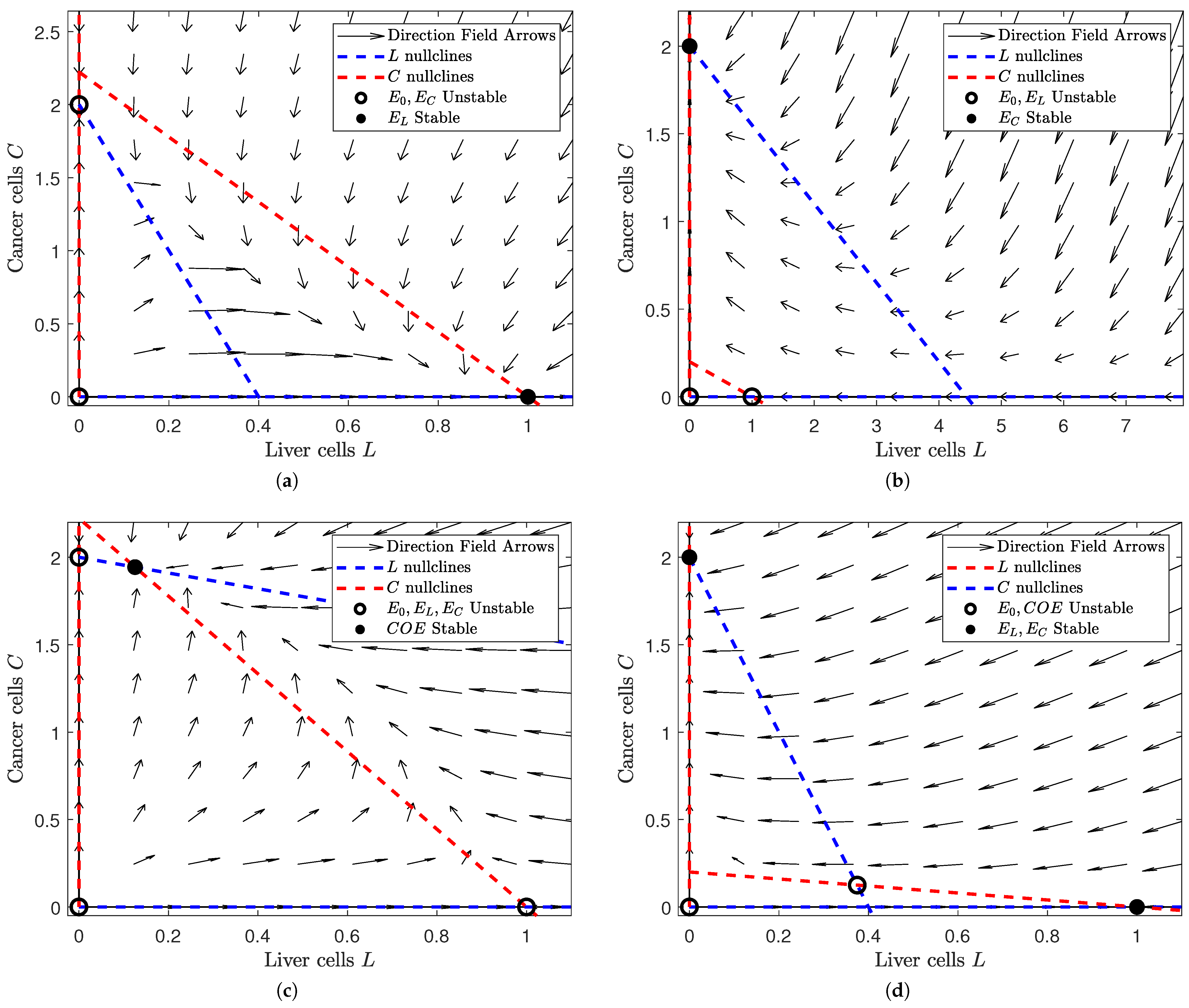
To visualize the behavior of our system in the absence of treatment (i.e., in Model (1)), we construct phase portraits in Figure 1. Phase portraits describe the behavior of solutions in different cases of parameters and initial conditions. Based on the existence and stability conditions of the equilibria in Table 3, we create a phase portrait for each possible collection of stable/unstable equilibrium points (differentiating between collections of equilibria when an equilibrium point changes stability). We find four possible states, each of which has a corresponding subfigure in Figure 1.

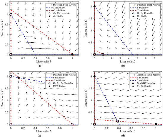
Figure 1. Depiction of the phase space of Model (1) for different values of ${\gamma }_L$ and ${\gamma }_C$. Note that the number of equilibria and their respective stability change as we alter ${\gamma }_L$ and ${\gamma }_C$. In each subfigure, a filled black dot indicates a stable equilibrium and a hollow black circle indicates an unstable equilibrium. The dashed red lines denote the L nullclines and the dashed blue ones the C nullclines. In all of the subfigures, the liver cells are on the horizontal axis and the cancer cells on the vertical. The figure was generated in MATLAB^®, with parameter values $K_L=1,K_C=2,\mu =0,$ and ${\lambda }_L={\lambda }_C=1$. We set the values of ${\gamma }_L$ and ${\gamma }_C$ to either $0.45$ or 5 (depending on the case we are interested in). (a) A view of the phase space where ${\gamma }_L=5$ and ${\gamma }_C=0.45$. Note that the liver-only equilibrium is the only stable steady state. (b) A view of the phase space where ${\gamma }_L=0.45$ and ${\gamma }_C=5$. Note that the cancer-only equilibrium is the only stable equilibrium. (c) A view of the phase space where ${\gamma }_L={\gamma }_C=0.45$. Note that the coexistence equilibrium is the only stable steady state. (d) A view of the phase space where ${\gamma }_L={\gamma }_C=5$. Note that the liver-only and cancer-only equilibria are stable while the trivial and coexistence equilibria are unstable.

In Figure 1, we notice that the number and stability of solutions are dependent on the relative values of ${\gamma }_L$ and ${\gamma }_C$. In Figure 1a, we see that the “liver-win” scenario is locally asymptotically stable when the influence of liver cells is large and that of cancer cells is small (i.e., ${\gamma }_L>1$ and ${\gamma }_C<1$). Similarly, Figure 1b shows us that the “cancer-win” scenario is locally asymptotically stable when cancer cell influence is high and liver cell influence is low (${\gamma }_L<1$ and ${\gamma }_C>1$). However, if the influence of both is low (${\gamma }_L,{\gamma }_C<1$), we see that a coexistence scenario is both possible and stable in Figure 1c. This suggests that the interaction between the liver cell and cancer cell populations is limited and their growth/death is mostly independent of the size of the other population. Finally, Figure 1d shows us that our coexistence scenario is no longer stable when liver cell and cancer cell influence are high (${\gamma }_L,{\gamma }_C>1$). Instead, both the “liver-win” and “cancer-win” scenarios are locally stable. This tells us that slight changes in initial conditions could result in drastically different outcomes.

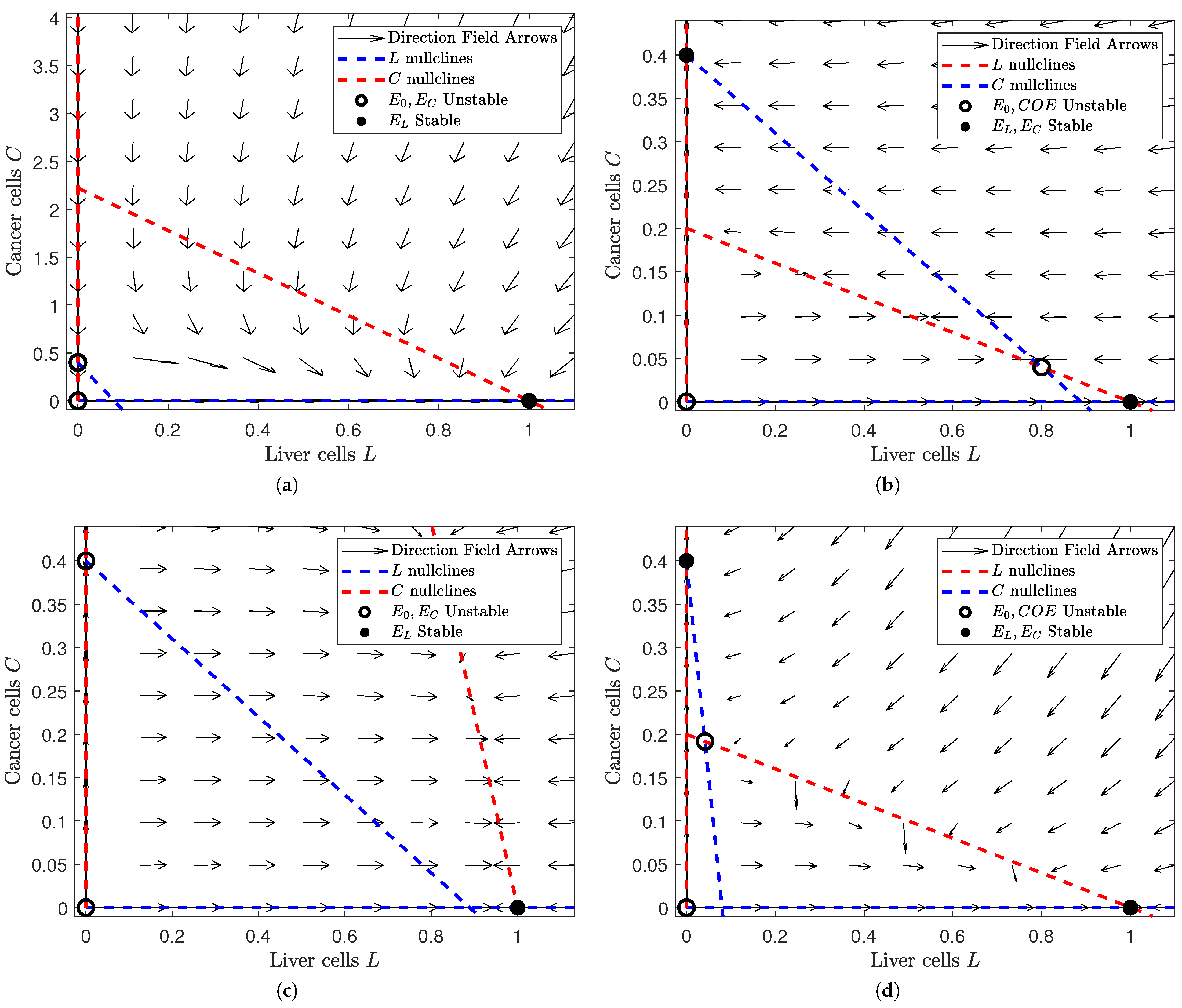
To observe the changes in stability once treatment is applied, we create phase portraits when $\mu >0$. Figure 2 uses Model (3), the equilibrium points (with their existence and stability conditions) from Table 4, and the same parameter values as Figure 1 to construct a phase portrait when $\mu =0.8$.

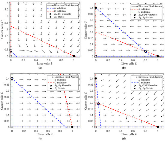
Figure 2. Depiction of the phase space of Model (3) for different values of ${\gamma }_L$ and ${\gamma }_C$ at $\mu =0.8$. Note that we choose the same values of ${\gamma }_L$ and ${\gamma }_C$ as in Figure 1: ${\gamma }_L=0.45,5$ and ${\gamma }_C=0.45,5$. This gives us four subfigures, each of which corresponds to a scenario in Figure 1 after treatment is applied. In each subfigure, a filled black dot indicates a stable equilibrium and a hollow black circle indicates an unstable equilibrium. The dashed red lines denote the L nullclines and the dashed blue ones the C nullclines. In all of the subfigures, the liver cells are on the horizontal axis and the cancer cells on the vertical. The figure was generated in MATLAB^®, with parameter values $K_L=1,K_C=2,$ and ${\lambda }_L={\lambda }_C=1$. We set the values of ${\gamma }_L$ and ${\gamma }_C$ to either $0.45$ or 5 (depending on the case we are interested in). (a) A view of the phase space where ${\gamma }_L=5$ and ${\gamma }_C=0.45$. Note that the liver-only equilibrium is the only stable steady state. This is no difference from Figure 1a. (b) A view of the phase space where ${\gamma }_L=0.45$ and ${\gamma }_C=5$. Note that the liver-only and cancer-only equilibria are stable while the trivial and coexistence equilibria are unstable. This is different from Figure 1b, where the cancer-only scenario was globally stable. (c) A view of the phase space where ${\gamma }_L={\gamma }_C=0.45$. Note that the liver-only equilibrium is globally stable. This is different from Figure 1c, where the coexistence equilibrium was globally stable. (d) A view of the phase space where ${\gamma }_L={\gamma }_C=5$. Note that the liver-only and cancer-only equilibria are stable while the trivial and coexistence equilibria are unstable. This is the same as in Figure 1d, although we notice a larger field of attraction for the liver-only equilibrium.

In Figure 2, we observe how the phase plane changes when we introduce treatment. Figure 2a changes the least between Figure 1 and Figure 2. The liver-only equilibrium is globally stable in both scenarios. This makes sense because healthy cells should prevail when their influence is greater, regardless of the presence of treatment. However, Figure 2b,c have a dramatic change in stability. In Figure 2b, the cancer cells have higher influence than the healthy cells. Without treatment, this would mean that the cancer cells would always win. Yet when treatment is added, the unstable coexistence equilibrium is introduced and both the liver-only and cancer-only equilibria become locally stable. This implies that treatment “balances the playing field" for healthy cells so that they can prevail under the right initial conditions. Comparatively, we lose an equilibrium in Figure 2c. Figure 2c shows us the behavior of solutions when the influence of both populations is small. While the coexistence equilibrium is stable without treatment, the coexistence equilibrium disappears and the liver-only equilibrium becomes stable once we apply treatment. This means that treatment boosts the influence of healthy cells so that they can eradicate the otherwise lingering cancer when this cancer is weak. Lastly, we notice a subtle shift in Figure 2d. Figure 2d shows us when both healthy and cancerous cells are aggressive. Both with and without treatment, the liver-only and cancer-only equilibria are stable while the coexistence equilibrium is unstable. However, we notice a larger basin of attraction for the liver-only equilibrium after treatment is added. This implies that a patient is more likely to be cancer-free with treatment than without treatment.

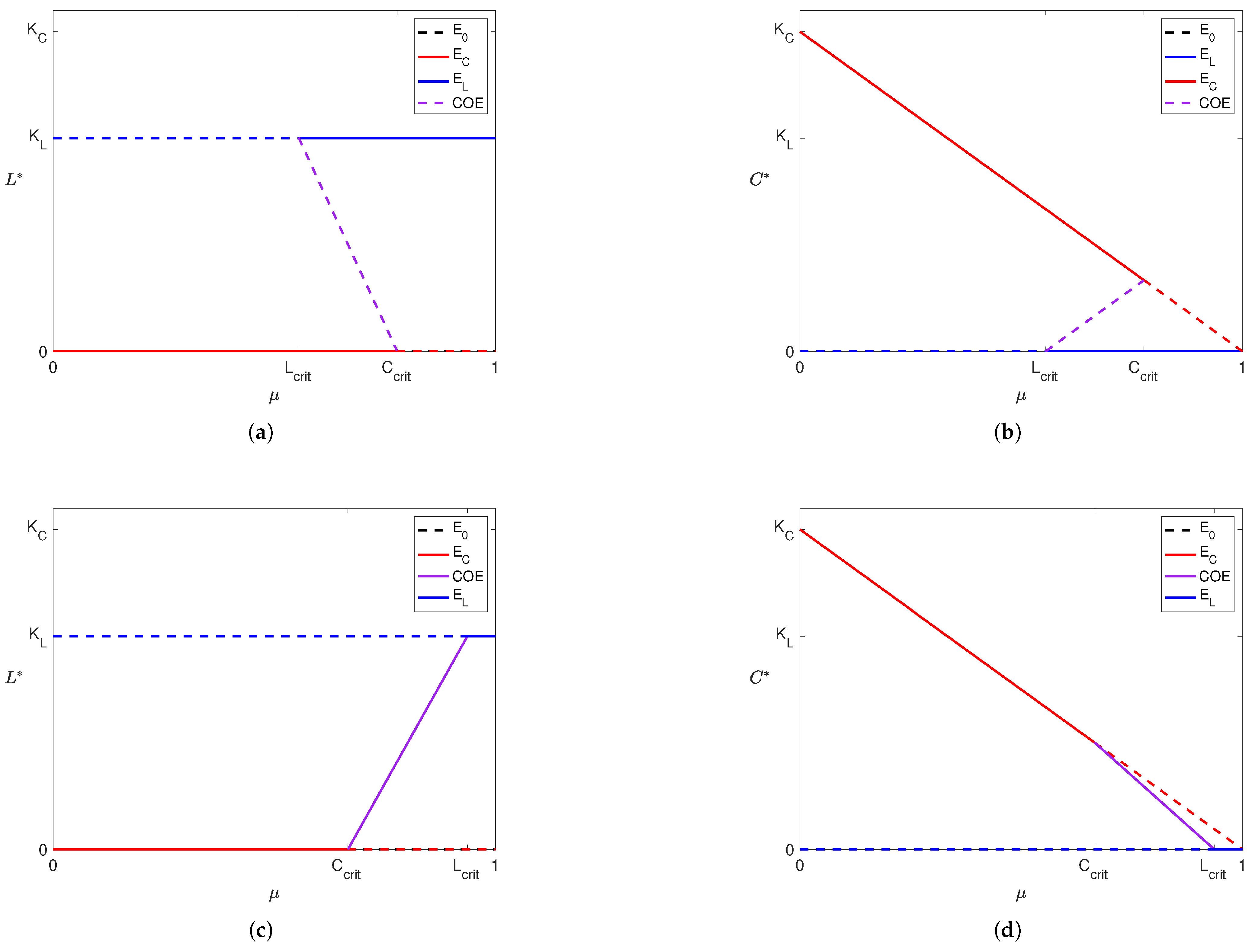
Due to inherent inaccuracies in data, we want to observe how variations in parameter values can change the stability of our solutions. Particularly, we use a bifurcation diagram to visualize the change in the outcome from Model (3) as we change the amount of treatment. So, we construct the following bifurcation diagram for Model (3) to observe how the stability of our solutions changes as $\mu$ increases.

In Figure 3, we see that the stability of our equilibria changes as $\mu$ increases. When influence of both liver cells and cancer cells is high (Figure 3a,b; ${\gamma }_L{\gamma }_C>1$) or low (Figure 3c,d; ${\gamma }_L{\gamma }_C<1$), we see that the cancer-wins scenario is stable for small $\mu$ values and the liver-wins scenario is stable for large $\mu$. While a coexistence scenario is stable when influence is low for both populations, this is not the case when the influence of both populations is high. In a patient that exists in the scenarios presented in Figure 3c,d, treatment administration at a level between $C_{crit}$ and $L_{crit}$ makes the tumor benign. Clinicians have effective procedures for clearing benign tumors, but such procedures go beyond the scope of this paper. Therefore, this level represents the minimal treatment for a patient of that profile. Similarly, for a patient with a more aggressive tumor (i.e., a larger value of ${\gamma }_C$), this “minimal treatment” could result in clearing the tumor or succumbing to it. We explore this further through numerical simulations described in Section 3.3.

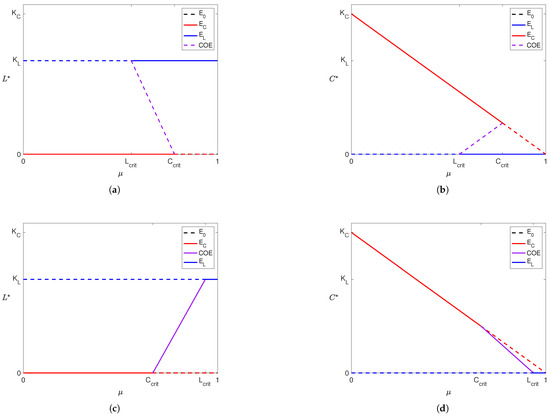
Figure 3. Depiction of bifurcation diagrams of Model (3) as the efficacy of the YAP gene treatment ($\mu$) is varied. Note that in (a,b), ${\gamma }_L=0.5$ and ${\gamma }_C=3$ so ${\gamma }_L{\gamma }_C>1$, and in (c,d) ${\gamma }_L{\gamma }_C<1$ since ${\gamma }_L=0.2$ and ${\gamma }_C=2$. The rest of the parameters were fixed across all cases. For each subfigure, solid lines indicate a stable equilibrium and dashed lines indicate an unstable equilibrium. The $E_0$ equilibrium is present and unstable in all four subfigures and is denoted by dashed black lines (although it appears hidden as it coincides with the x-axis of each subfigure and is simultaneously covered by other equilibria). Purple lines represent the coexistence equilibrium. Dashed and solid red lines denote the cancer boundary equilibrium ($E_C$) and dashed and solid blue lines denote the liver boundary equilibrium ($E_L$).

3.2. Data Fitting

To perform simulations using our model, we need numeric values for model parameters. In this subsection, we present parameter values estimated using the methods detailed in Section 2.3. When numerically solving both Problems (6) and (7), we take $\alpha$, the tracking weight, to be 100 and $\beta$, the regularization weight, to be 1. This places emphasis on minimizing the sum of squared errors between our model outputs and the data. We used data from Koniaris et al. [18] to fit ${\lambda }_L$, since this experiment measured the regrowth of mouse livers after two-thirds partial hepatectomy and found ${\lambda }_L$ to be about $2.17$ (week⁻¹), with an approximate relative $l^2$ error percentage of $12.5\%$. Then, using this value, we solved Problem (7) to estimate the ${\lambda }_C$ and ${\gamma }_L$ using data from Anton et al. [54]. This set of parameters resulted in an approximate relative $l_2$ error percentage of $10.4\%$ between the simulated cancer curve and normalized data from Anton et al. [54]. Table 5 contains “best fit” parameter values estimated through literature review and data-fitting for Model (3). Multiple experiments with the MultiStart algorithm in MATLAB® while varying initial guesses repeatedly found this set of parameters to minimize the functionals in Problems (6) and (7).

Table 5. Model (3) parameter values estimated from literature and data-fitting with units.

Parameters	Description	Value	Units
${\lambda }_L$	Healthy cell proliferation rate	$2.17$	1/week
${\lambda }_C$	Cancer proliferation rate	$1.81$	1/week
$K_L$	Healthy liver volume	1500	mm3
$K_C$	Tumor carrying capacity	7500	mm3
${\gamma }_L$	Influence of healthy liver cells on cancer cells’ access to resources	$0.640$	dimensionless

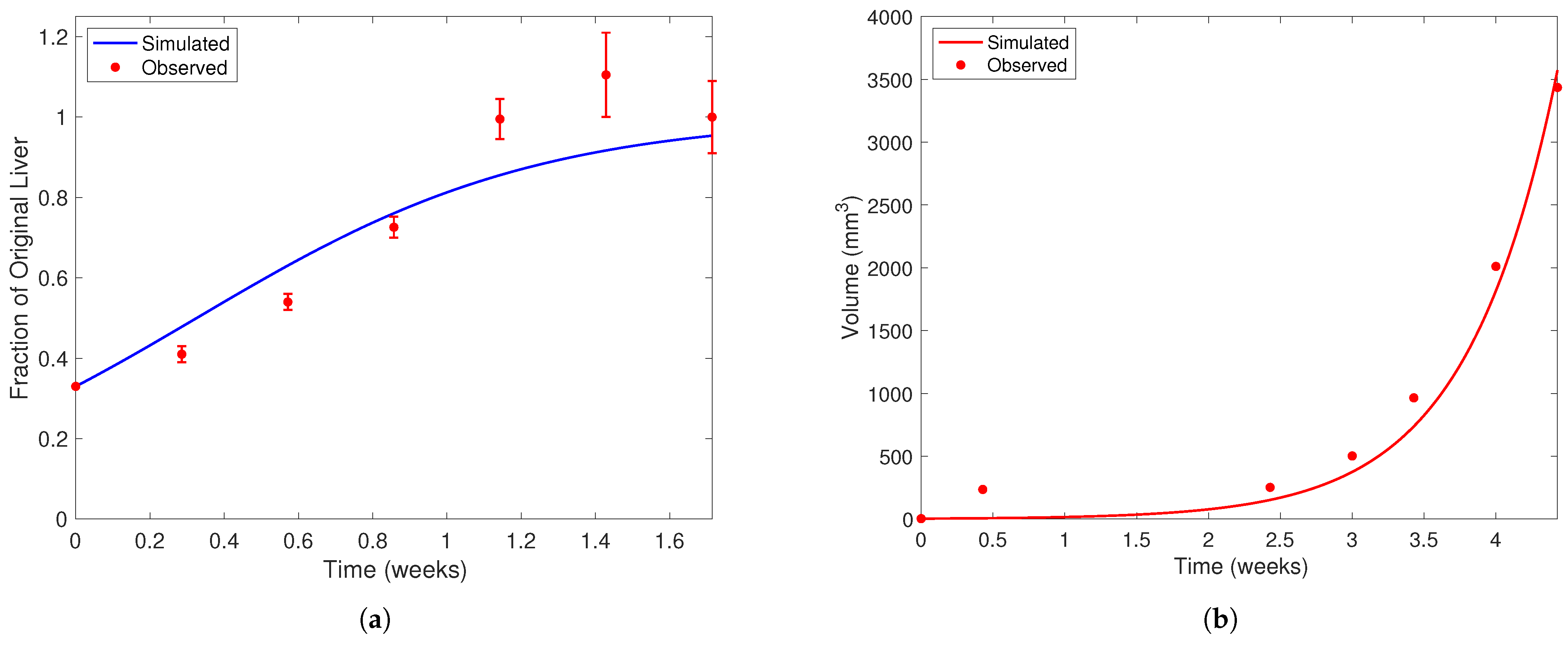
In Figure 4, we present the solution curves of Model (4) and Model (5) using the “best fit” parameter from Table 5 against the data used to find them. Figure 4a depicts the healthy cell population over time using the value of ${\lambda }_L$ found from solving Problem (6). The filled red dots with error bars are the data points from the Koniaris et al. [18] experiment. In Figure 4b, we present the tumor volume using the parameters in Table 5 against the Anton et al. data [54]. When solving Problem 7, recall that we use Model (5) as the constraint rather than Model (3) and that Model (5) is a reduced version of Model (3) where $C\approx 0$. We also take ${\gamma }_C=0$ during the parameter estimation process, as we cannot estimate this parameter from the available literature or data. This set of parameters resulted in a relative $l^2$ error percentage of $10.4\%$ between the simulated tumor volume and experimental data. Most of this error comes from the data point at Day 3, since our model could not replicate the very fast growth at the start of the experiment. However, our model and parameter set does well to track the rest of the experimental data.

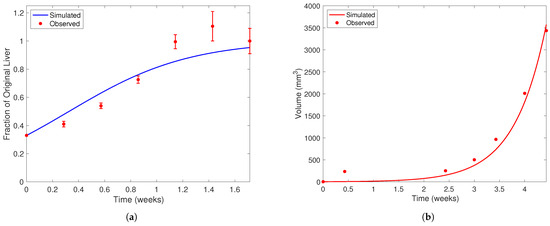
Figure 4. Liver and cancer population curves using the “best fit” parameters from Table 5. In each subfigure, the horizontal axis represents time (weeks) and the vertical liver volume (mm³). Note the difference in scale on the vertical axis between each subfigure. Filled red dots represent experimental data and solid curves represent simulated population curves. In (a), data is taken from Koniaris et al. [18] in mice after two-thirds partial hepatectomy. Error bars represent the range of values Koniaris et al. [18] measured from 10 mice studied in their experiment. In (b), data of tumor volume from a representative mouse over time is taken from Anton et al. [54]. The dark blue curve in (a) represents the healthy liver population and the red curve in (b) the cancerous population. When fitting to the Anton et al. [54] dataset, we assume the initial liver population is at its carrying capacity and ignore the quadratic limiting term in the $dC/dt$ equation. We also impose that, at the 3-week time point, a mouse with the YAP genes “knocked out” in healthy cells will have a tumor that is double the size of a mouse with wild-type liver cells [12].

3.3. Numerical Results

In this subsection, a set of numerical simulations is presented to support the theoretical results presented in Section 3.1 and to show the applicability of Model (3) after validating it in Section 3.2. We use the parameters estimated from the literature and through data-fitting (listed in Table 1) and vary the values of ${\gamma }_C$ and $\nu$ to represent various patient and treatment profiles. Simulations using larger values of ${\gamma }_C$ represent patients with more aggressive tumors, while those with smaller values represent less aggressive tumors. Mathematically, we take ${\gamma }_C>{\displaystyle \frac{1}{{\gamma }_L}}$ to represent more aggressive tumors and ${\gamma }_C\le {\displaystyle \frac{1}{{\gamma }_L}}$ to represent less aggressive tumors. Similarly, larger values of $\nu$ correspond to patients receiving larger doses of treatment. Conversely, $\nu =0$ represents no treatment. We also numerically find the minimal amount of treatment physicians should prescribe for patients with aggressive tumors. Through our numerical simulations, we aim to provide physicians with insight into the usage of YAP hyperactivation therapy to treat HCC.

Recalling the formulation of Model (3), we impose the condition ${\gamma }_C>1>{\gamma }_L$. Through our model validation, we found ${\gamma }_L=0.640$, but we were not able to estimate the value of ${\gamma }_C$ from any available data or recent literature. Combining our results from Table 3 and Table 5, we note that, without treatment, the $E_L$ equilibrium is always unstable, the $E_C$ equilibrium is stable if and only if ${\gamma }_C>0.2$, and the coexistence only exists in the scenario where ${\gamma }_C<0.2$ but will be stable if it does. However, due to the constraint we imposed on Model (3), we can only achieve a state where the cancer population reaches its carrying capacity and the healthy liver cells die out. Note that we intentionally break the constraint for some of our simulations without treatment in Figure 5.

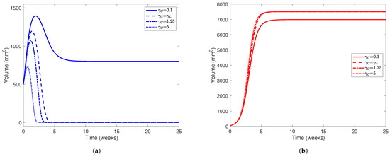
Figure 5. Liver (a) and tumor (b) populations using the parameter values in Table 5 while varying ${\gamma }_C$. In both subfigures, line styles correspond to different values of ${\gamma }_C$: solid lines represent simulations using ${\gamma }_C=0.1$, dashed lines ${\gamma }_C={\gamma }_L$, dotted-dashed lines ${\gamma }_C=1.25$, and dotted lines ${\gamma }_C=5$. The initial healthy liver volume was 500 mm³ and the initial tumor volume was 50 mm³ and ${\lambda }_L=2.17$, ${\lambda }_C=1.81$, $K_L=1500$, $K_C=7500$, and ${\gamma }_L=0.640$. Note the difference in scale between the y-axes on each subfigure.

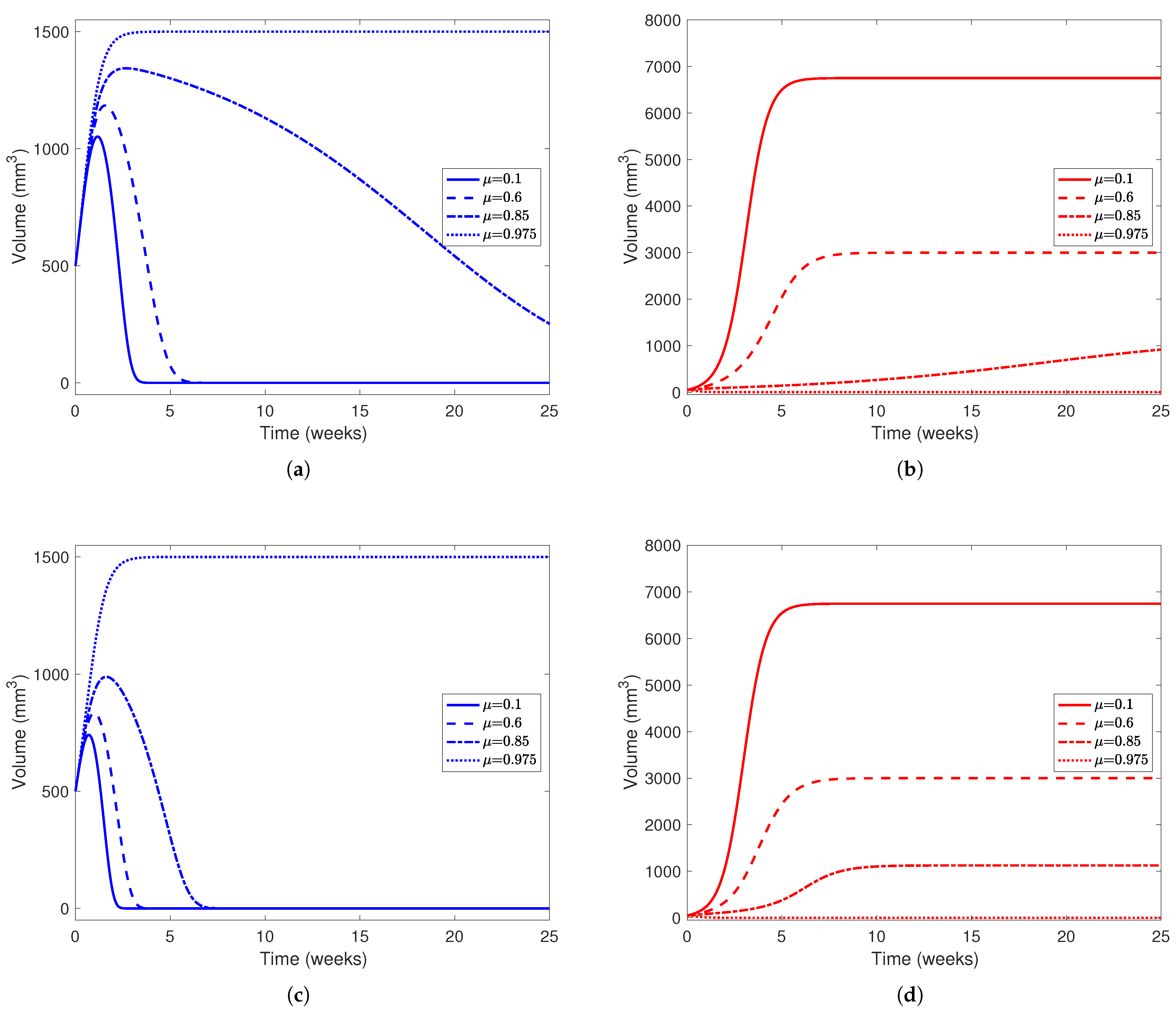
In Figure 5, we present simulations of various patient profiles after partial hepatectomy with various values of ${\gamma }_C$ (namely ${\gamma }_C=0.1,{\gamma }_L,1.25,$ and 5). The choices of ${\gamma }_C$, although arbitrary, are plausible when considering that tumors use more resources and are more aggressive in their acquisition of resources than normal hepatocytes. While the cases where ${\gamma }_C=0.1$ and ${\gamma }_C={\gamma }_L$ do not satisfy the condition we placed on our model (${\gamma }_C>1>{\gamma }_L$), the importance of the condition itself is evident when comparing the simulation using ${\gamma }_C=0.1$ with simulations using larger values of ${\gamma }_C$. Using this set of parameter values, we only expect to see a “coexistence” scenario between the healthy and cancerous populations when ${\gamma }_C=0.1$. In all simulations, we set $\nu =0$ since we want to investigate the competition between healthy and cancerous hepatocytes in the absence of treatment first. For our initial conditions, we take $L_0=500$ mm³ and $C_0=50$ mm³ to represent a patient who has undergone partial hepatectomy (PH) where nearly two-thirds of their liver was removed but a relatively small tumor still remains.

From Figure 5, we find that the value of ${\gamma }_C$ has a major impact on the outcome of the “patient.” In all simulations, the cancer outgrows the tumor and reaches its carrying capacity or a size comparable to it, while the healthy population always dies out when ${\gamma }_C>1$. Only in the case where ${\gamma }_C=0.1$ does the liver population stabilize at 800 mm³, though the tumor size stabilizes at around 7000 mm³. The magnitude of ${\gamma }_C$ also has a noticeable affect on how quickly the healthy population declines to 0. As ${\gamma }_C$ increases, we notice that the healthy population’s volume peaks earlier in the experimental window and at a smaller value. For example, when ${\gamma }_C=1.25$, the healthy liver volume peaks at 1050 mm³ about 1.5 weeks after PH, but when ${\gamma }_C=5$, this volume peaks at about 700 mm³ only 0.725 weeks (about 5 days) after PH. This indicates that for a patient with a more aggressive tumor, YAP hyperactivation therapy must be started soon after they undergo PH.

In Model (3), we also incorporate treatment, where YAP is hyperactivated to boost hepatocytes and other healthy cells’ ability to compete against cancerous cells. In the model, $\mu$ represents a dimensionless measure of drug effect; for our simulations, we take $\mu =0.1,0.6,0.85$, and $0.975$ to represent the effect of low to high drug dosages. For the rest of the parameters, we use the values listed in Table 5 found from the literature and data-fitting. Since ${\gamma }_C$ could not be found, we take ${\gamma }_C=1.5$ and ${\gamma }_C=5$ to represent patients with varying levels of tumor aggression, and for initial conditions, we take $L_0=500$ mm³ and $C_0=50$ mm³ to represent a patient who has undergone two-thirds PH and has a small tumor remaining after the procedure. With these parameters, we have $L_{crit}=0.872$ and $C_{crit}=0.867$ when ${\gamma }_C=1.5$ or $C_{crit}=0.96$ when ${\gamma }_C=5$. From our results in Section 3.1 and Table 4, if ${\gamma }_C=5$, we know the scenario where the healthy liver cells outcompete and defeat the cancerous cells is stable if $\mu >C_{crit}$ and the opposite scenario (where the cancerous cells win) is stable if $\mu <L_{crit}$. Similarly, if ${\gamma }_C=1.5$, we expect the healthy liver cells to win when $\mu >L_{crit}$ and the cancer cells to win when $\mu <C_{crit}$. We can achieve the coexistence scenario when $C_{crit}<\mu <L_{crit}$ for patients with less aggressive tumors (in our case, ${\gamma }_C=1.5$). For patients in this scenario (where the tumor is relatively less aggressive in its recruitment and consumption of resources from the environment), we can attempt to administer “minimal treatment” corresponding to $0.867<\mu <0.872$ and allow the patient’s immune system to fight off a smaller, weaker tumor. In patients with more aggressive tumors (${\gamma }_C=5$), we expect the coexistence scenario when $L_{crit}<\mu <C_{crit}$, but we cannot physically achieve coexistence between cancerous and healthy cells. We explore this phenomenon further in Figure 8.

In Figure 6, we see that the treatment has a bigger effect on the outcome of the cancer cell population than the healthy cells. In Figure 6a, we find that higher drug dosage, even when not enough to clear the tumor, flattens the decay of the healthy cell population. For example, when $\mu =0.85$, the healthy cell population peaks around 1350 mm³ and takes more than 20 weeks to decay to 0, while when $\mu =0.6$, the healthy population peaks around 1150 mm³ and decays within 5 weeks after its peak. This further reinforces the fact that patients, under this parameter configuration, need a high dose of drug to guarantee clearing a tumor. In Figure 6b, even in scenarios where the cancer population outcompetes the healthy cells, the end state of the cancer cell decreases as drug effect increases. This is evident from Table 4, where the end state of the cancer population in the cancer-win equilibrium is $K_C(1-\mu )$. As mentioned earlier, the tumor is only cleared in the simulation with a “very high” drug effect ($\mu =0.975$) since this is the only simulation presented where $\mu >L_{crit}$. In Figure 6c,d, we investigate a patient with a more aggressive tumor (${\gamma }_C=5$) while using treatment to the same effect ($\mu =0.1,0.6,0.85,$ and $0.975$). While the end behavior does not change much between the simulations with a less aggressive tumor and a more aggressive tumor, in simulations with a more aggressive tumor, the healthy cell populations peak at a smaller volume and decay to 0 earlier in the experiment, as noted in Figure 5.

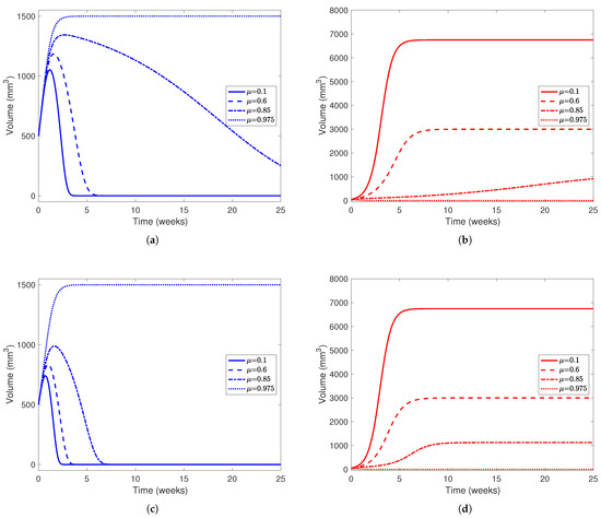
Figure 6. Liver and cancer population curves using parameters from Table 5 while varying $\mu$ between 0 and 1. For each subplot, the solid line represents no drug dosage ($\mu =0.1$), dashed lines a medium dose ($\mu =0.6$), dotted-dashed lines a high dose ($\mu =0.85$), and dotted lines a very high dose ($\mu =0.975$). Blue curves represent the healthy portion of the liver and red curves represent the cancerous portion of the liver. In (a,b), ${\gamma }_C=1.5$, representing a tumor that is not very aggressive, while in (c,d), ${\gamma }_C=5$, representing a much more aggressive tumor. In all subfigures, the initial healthy liver volume is 500 mm³ and the initial tumor volume is 50 mm³. This represents a patient who has undergone two-thirds PH but still has a small amount of cancerous cells left in their liver after the procedure and before YAP hyperactivation. In each subfigure, the horizontal axis represents time in weeks and the vertical liver volume.

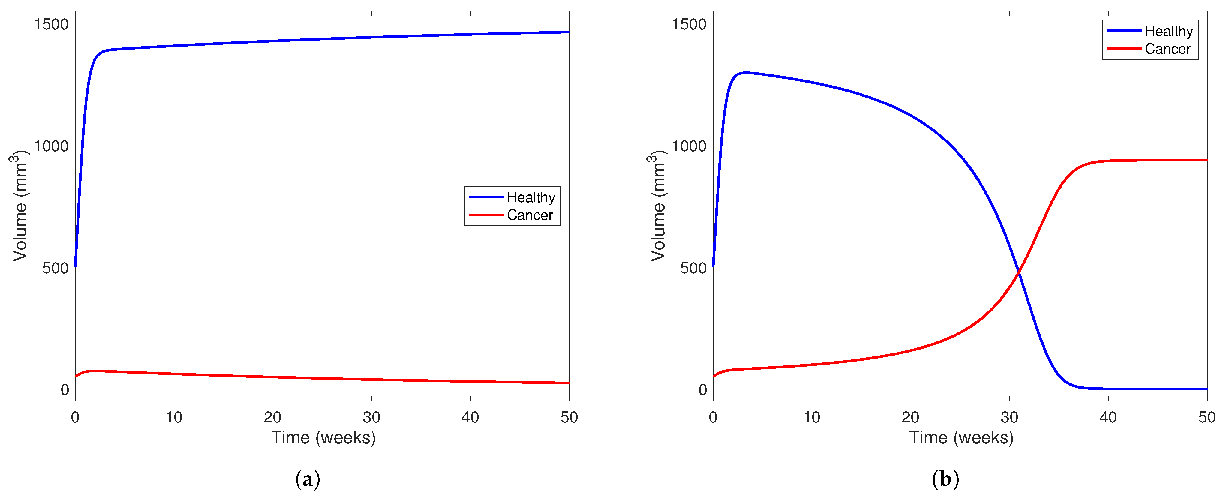
In Figure 7, we investigate the outcome of administering treatment between $L_{crit}$ and $C_{crit}$ in a patient with a “low-aggresion” tumor and in one who has a very aggressive tumor. We choose $\mu =0.875$ in both scenarios and use parameters from Table 5. We also take $L_0=500$ mm³ and $C_0=50$ mm³ to visualize a patient who has just undergone two-thirds PH, as in the other simulations presented in this section. In Figure 7a, the model predicts a scenario where the healthy part of the liver can outcompete the cancerous part with the help of treatment at this level. The treatment level ($\mu =0.875$) is near the lower end of the range between $L_{crit}=0.872$ and $C_{crit}=0.960$, meaning the treatment can potentially clear a tumor with low aggression. However, in Figure 7b, using the same parameter set, but taking ${\gamma }_C=2.5$ to represent a more aggressive tumor, we notice that the tumor still wins even with treatment.

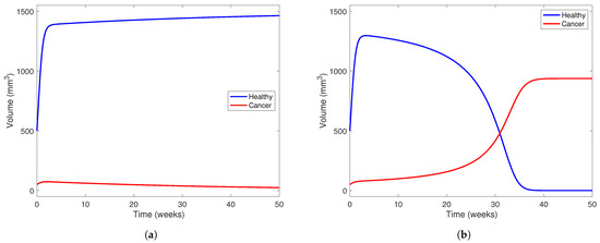
Figure 7. Liver and cancer population curves using parameters from Table 5 while taking $\mu =0.875$. Blue curves represent the healthy portion of the liver and red curves represent the cancerous portion of the liver. In (a), ${\gamma }_C=1.5$, representing a tumor that is not very aggressive, while in (b), ${\gamma }_C=2.5$, representing a more aggressive tumor. In both subfigures, the initial healthy liver volume is 500 mm³ and the initial tumor volume is 50 mm³. This represents a patient who has undergone two-thirds PH but still has a small amount of cancerous cells left in their liver after the procedure and before YAP hyperactivation. In each subfigure, the horizontal axis represents time in weeks and the vertical liver volume.

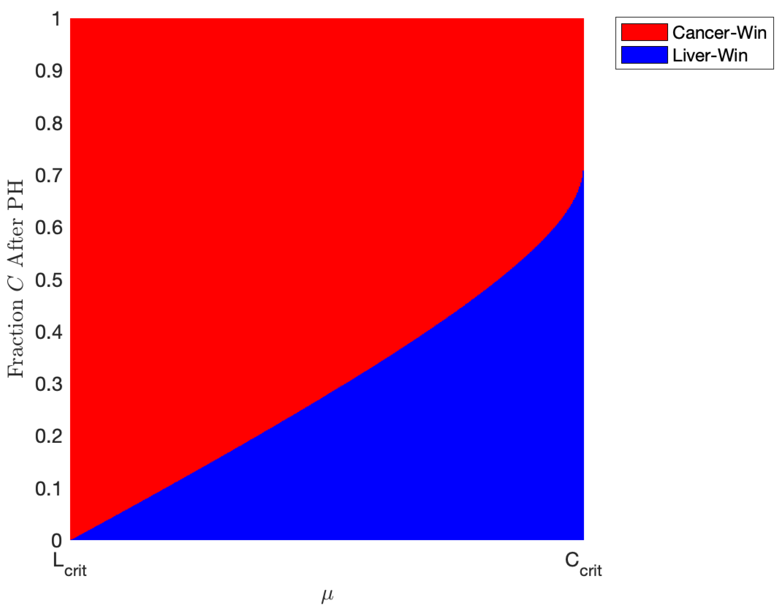
We explore this phenomenon further in Figure 8. Here, we take ${\gamma }_C=5$, representing a patient with an even more aggressive tumor. As described in Section 3.1 and Figure 2 and Figure 3, the coexistence scenario mathematically exists under our parameter set when $L_{crit}=0.872<\mu <0.960=C_{crit}$ but is not stable, meaning it cannot be plausibly achieved. However, in this parameter range, we have bistability, meaning either the “cancer-wins” or the “healthy-win” scenario can occur depending on the state of the liver when the YAP hyperactivation therapy is started. In Figure 8, we simulate the outcomes of our model using the parameters listed in Table 5, taking ${\gamma }_C=5$, while varying initial conditions of the model and varying $\mu$ between $L_{crit}$ and $C_{crit}$. For the initial conditions, we take a patient who has just undergone two-thirds PH, meaning $L_0+C_0={\displaystyle \frac{1}{3}}$; on the y-axis, we plot the fraction of the initial liver volume after PH that is tumor. Figure 8 represents the effects of administering minimal treatment for a patient with an aggressive tumor. In the plot, red represents a scenario where the cancer population wins, while the blue patch represents a scenario where the healthy liver cells outcompete and defeat the cancerous cells with the help of YAP hyperactivation. Using the parameters we found from validating our model, we conclude that a patient with an aggressive tumor may be treated with doses of a drug that has an effect of about 0.872 units, but only if the tumor volume after two-thirds PH is miniscule. Increasing the drug effect, $\mu$, results in being able to administer treatment in patients with a larger portion of their liver being cancerous after PH.

Figure 8. Plot indicating the outcome of various amount of treatment for patients with different amounts of tumor left after one-third partial hepatectomy (PH). Red indicates a “cancer-win” scenario and blue a “liver-win” scenario. The parameters are taken from Table 5 with ${\gamma }_C=5$ and $\mu$ varying between $L_{crit}$ and $C_{crit}$. This represents the minimal amount of treatment necessary for a patient to recover given our estimated parameters. Note that in this range of $\mu$, a scenario where there is both tumor and some “healthy” liver mathematically exists but is physically unachievable (see Table 4). Thus, we only have two scenarios where there is either only cancer or only “healthy” liver.

4. Discussion

A simple two-dimensional model was developed to model the dynamics of competition between normal hepatocytes and cancerous liver cells after partial hepatectomy. The model was then modified to incorporate the effect of YAP hyperactivation, a novel gene therapy that boosts the ability of non-cancerous hepatocytes to fight against and restrict the growth of a liver tumor. These models were then analyzed for their dynamical properties and validated against experimental data. Finally, a set of numerical simulations were presented where we applied the model to various patient and treatment scenarios and found that ${\gamma }_C$ is a critical parameter in predicting patient outcome. This study shows the following:

• Given the constraint imposed on Model (3), where ${\gamma }_L<1<{\gamma }_C$, the tumor is heavily favored to outcompete the healthy cells for resources and reach its carrying capacity, while nullifying the healthy cells in the absence of treatment.
• Literature review and data-fitting confirmed that the effect of the healthy liver cells on a tumor (${\gamma }_L$) without YAP hyperactivation is relatively small compared to the effect of a tumor on the liver (${\gamma }_C$).
• Although the number of steady states between Models (1) and (3) remain the same with and without treatment, the behavior of various equilibria change to favor the healthy liver cell population when treatment is incorporated.
• The minimal treatment profile needed to alter the end-behavior of the healthy and cancerous cell populations depends on the aggressiveness of the cancer and the size of the tumor. For non-aggressive tumors, a “medium” effect of treatment ($\mu$ between $C_{crit}$ and $L_{crit}$) is sufficient to make the tumor controllable. The exact values for this range depend on the patient. However, this same effectiveness of treatment is only useful to fight against aggressive tumors if the size of the tumor at the onset of treatment is small. Otherwise, a “high” effect of treatment is needed.
• From the estimated parameter set presented in Table 5, a high effect of treatment ($\mu >0.9$) is needed to fully eradicate cancer cells from the liver. However, if the patient has a tumor with a “normal” level of aggression (i.e., $1<{\gamma }_C\le {\displaystyle \frac{1}{{\gamma }_L}}$), physicians may prescribe a slightly lower dose of the drug and prescribe adjuvant therapies to fight off a smaller, weaker tumor.
• Even in scenarios where the drug alone is not enough to save a patient, in a patient with a less aggressive tumor, the healthy liver cell population will take longer to decay to 0 than in a patient with an aggressive tumor (i.e., a large value of ${\gamma }_C$), as presented in the numerical results and in Figure 6.
• The numerical value of ${\gamma }_C$ is an important indicator of a patient’s outcome and should be considered when prescribing YAP hyperactivation therapy; if ${\gamma }_C>{\displaystyle \frac{1}{{\gamma }_L}}\approx 1.563$, the patient is considered to have an aggressive tumor. In Figure 8, we show that patients with an aggressive tumor can be treated with “minimal” YAP hyperactivation after PH if only a small percentage of the liver after resection is cancerous.

Although we could complicate Model (3) to incorporate immune cells [28], various treatment regimes, or spatial heterogeneity, the model still effectively captures the dynamics of competition between healthy liver and cancer cells while being simple to analyze and implement. We provided insight into the usage of a novel, non-invasive therapy for primary liver cancers by incorporating this type of treatment into the model. We also found that the aggressiveness of the tumor, a patient-specific parameter, is crucial to quantifying the prognosis of patients and in determining the potential YAP hyperactivation treatment plan. A potential extension of this work is to explore more strategies to tailor YAP hyperactivation therapy to various types of patients using biomarkers such as age, gender, and race. Other future areas of interest include combining YAP activation with other treatment strategies, optimizing patient-specific treatment schedules, and exploring potential tumor resistance to sub-optimal treatment administration.

Appendix A.1. Model (3) Linearization

The linearized version of Model (3) is given by the Jacobian matrix below:

$$\mathbf{J}(L^{*},C^{*})=\left[\begin{array}{cc}-{\displaystyle \frac{{\lambda }_L{L}^{*}}{K_L}}+{\lambda }_L\left(1-{\displaystyle \frac{L^{*}+{\gamma }_C{C}^{*}}{K_L}}\right)& -{\displaystyle \frac{{\lambda }_L{\gamma }_C}{K_L}}{L}^{*}\\ -{\displaystyle \frac{{\lambda }_C{\gamma }_L}{K_C}}{C}^{*}& {\lambda }_C(1-\mu )\left(1-{\displaystyle \frac{{\gamma }_L{L}^{*}+C}{K_C(1-\mu )}}\right)-{\displaystyle \frac{{\lambda }_C{C}^{*}}{K_C}}\end{array}\right].$$

Appendix A.2. Extinction Scenario

The extinction scenario ($E_0$) occurs always and has Jacobian

$$\mathbf{J}(0,0)=\left[\begin{array}{cc}{\lambda }_L& 0\\ 0& {\lambda }_C(1-\mu )\end{array}\right].$$

The eigenvalues of this matrix are ${\lambda }_1={\lambda }_L$ and ${\lambda }_2={\lambda }_C(1-\mu )$. Clearly, ${\lambda }_1,{\lambda }_2>0$, meaning the $E_0$ equilibrium is unstable always.

Appendix A.3. Liver-Win Scenario

The liver-win scenario ($E_L$) always occurs and has the associated Jacobian

$$\mathbf{J}(L^{*},C^{*})=\left[\begin{array}{cc}-{\lambda }_L& -{\lambda }_L{\gamma }_C\\ 0& {\lambda }_C\left(1-{\displaystyle \frac{{\gamma }_L{K}_L}{K_C}}-\mu \right)\end{array}\right].$$

This matrix has eigenvalues ${\lambda }_1=-{\lambda }_L$ and ${\lambda }_2={\lambda }_C\left(1-{\displaystyle \frac{{\gamma }_L{K}_L}{K_C}}-\mu \right)$. This equilibrium is stable if ${\displaystyle \frac{{\gamma }_L{K}_L}{K_C}}+\mu >1$ and a saddle point when ${\displaystyle \frac{{\gamma }_L{K}_L}{K_C}}+\mu <1$.

Appendix A.4. Cancer-Win Scenario

The cancer-win scenario ($E_C$) occurs always and has the associated Jacobian

$$\mathbf{J}(L^{*},C^{*})=\left[\begin{array}{cc}{\lambda }_L\left(1-{\displaystyle \frac{{\gamma }_C{K}_C(1-\mu )}{K_L}}\right)& 0\\ -{\lambda }_C{\gamma }_L(1-\mu )& -{\lambda }_C(1-\mu )\end{array}\right].$$

This matrix has eigenvalues ${\lambda }_1={\lambda }_L\left(1-{\displaystyle \frac{{\gamma }_C{K}_C(1-\mu )}{K_L}}\right)$ and ${\lambda }_2=-{\lambda }_C(1-\mu )$. This equilibrium is stable when ${\displaystyle \frac{K_C}{{\gamma }_C{K}_L}}+\mu <1$ and is a saddle point when ${\displaystyle \frac{K_C}{{\gamma }_C{K}_L}}+\mu >1$.

Appendix A.5. Coexistence Scenario

The coexistence scenario (COE) occurs only when ${\gamma }_C>{\displaystyle \frac{K_L}{K_C(1-\mu )}}$ and ${\gamma }_L>{\displaystyle \frac{K_C(1-\mu )}{K_L}}$ or ${\gamma }_C<{\displaystyle \frac{K_L}{K_C(1-\mu )}}$ and ${\gamma }_L<{\displaystyle \frac{K_C(1-\mu )}{K_L}}$. Note that ${\gamma }_C>{\displaystyle \frac{K_L}{K_C(1-\mu )}}$ and ${\gamma }_L>{\displaystyle \frac{K_C(1-\mu )}{K_L}}$ imply $a>1$ and ${\gamma }_C<{\displaystyle \frac{K_L}{K_C(1-\mu )}}$ and ${\gamma }_L<{\displaystyle \frac{K_C(1-\mu )}{K_L}}$ imply $a<1$. The COE has Jacobian

$$\begin{array}{cc}\hfill \mathbf{J}(L^{*},C^{*})& =\left[\begin{array}{cc}-{\lambda }_L\left({\displaystyle \frac{K_L-{\gamma }_C{K}_C(1-\mu )}{K_L(1-{\gamma }_L{\gamma }_C)}}\right)& -{\displaystyle \frac{{\lambda }_L{\gamma }_C(K_L-{\gamma }_C{K}_C(1-\mu ))}{K_L(1-{\gamma }_L{\gamma }_C)}}\\ -{\displaystyle \frac{{\lambda }_C{\gamma }_L(K_C(1-\mu )-{\gamma }_L{K}_L)}{K_C(1-{\gamma }_L{\gamma }_C)}}& -{\lambda }_C\left({\displaystyle \frac{K_C(1-\mu )-{\gamma }_L{K}_L}{K_C(1-{\gamma }_L{\gamma }_C)}}\right)\end{array}\right]\hfill \\ \hfill & =\left[\begin{array}{cc}-{\displaystyle \frac{{\lambda }_L}{K_L}}{L}^{*}& -{\displaystyle \frac{{\lambda }_L{\gamma }_C}{K_L}}{C}^{*}\\ -{\displaystyle \frac{{\lambda }_C{\gamma }_L}{K_C}}{L}^{*}& -{\displaystyle \frac{{\lambda }_C}{K_C}}{C}^{*}\end{array}\right]\hfill \\ \hfill & =\left[\begin{array}{cc}-{\rho }_L{L}^{*}& -{\gamma }_C{\rho }_L{C}^{*}\\ -{\gamma }_L{\rho }_C{L}^{*}& -{\rho }_C{C}^{*}\end{array}\right],\hfill \end{array}$$

where ${\rho }_L={\displaystyle \frac{{\lambda }_L}{K_L}}$ and ${\rho }_C={\displaystyle \frac{{\lambda }_C}{K_C}}$. This matrix has eigenvalues

$$\begin{array}{cc}\hfill & {\lambda }_1={\displaystyle \frac{1}{2}}\left[-({\rho }_L{L}^{*}+{\rho }_C{C}^{*})-\sqrt{{({\rho }_L{L}^{*}+{\rho }_C{C}^{*})}^2-4{\rho }_L{\rho }_C(1-{\gamma }_L{\gamma }_C)L^{*}{C}^{*}}\right],\hfill \\ \hfill & {\lambda }_2={\displaystyle \frac{1}{2}}\left[-({\rho }_L{L}^{*}+{\rho }_C{C}^{*})+\sqrt{{({\rho }_L{L}^{*}+{\rho }_C{C}^{*})}^2-4{\rho }_L{\rho }_C(1-{\gamma }_L{\gamma }_C)L^{*}{C}^{*}}\right].\hfill \end{array}$$

Since $L^{*},C^{*}>0$, ${\lambda }_1<0$ always. Next, ${\lambda }_2<0$ if

$$\begin{array}{cc}\hfill {\rho }_L{L}^{*}+{\rho }_C{C}^{*}& >\sqrt{{({\rho }_L{L}^{*}+{\rho }_C{C}^{*})}^2-4{\rho }_L{\rho }_C(1-{\gamma }_L{\gamma }_C)L^{*}{C}^{*}}\hfill \\ \hfill {({\rho }_L{L}^{*}+{\rho }_C{C}^{*})}^2& >{({\rho }_L{L}^{*}+{\rho }_C{C}^{*})}^2-4{\rho }_L{\rho }_C(1-{\gamma }_L{\gamma }_C)L^{*}{C}^{*}\hfill \\ \hfill 0& >-4{\rho }_L{\rho }_C(1-{\gamma }_L{\gamma }_C)L^{*}{C}^{*}\hfill \\ \hfill 0& <1-{\gamma }_L{\gamma }_C\hfill \\ \hfill \Rightarrow {\gamma }_L{\gamma }_C& <1.\hfill \end{array}$$

So, when the COE exists, it is stable if ${\gamma }_L{\gamma }_C<1$ and an unstable saddle point otherwise.

Appendix A.6. Global Stability

The Poincaré–Bendixson Theorem states that, for a two-dimensional system of ODEs, all of its solutions must grow without bound, approach a closed orbit, or asymptotically approach an equilibrium in the long term. By process of elimination, we will show that all solutions of Model (3) approach an equilibrium.

To show that solutions are bounded, we will construct a “bounding box” (or trapping region) D such that all solutions must enter D and cannot exit. Note that for ${\displaystyle \frac{dL}{dt}}<0$, ${\lambda }_C\left(1-{\displaystyle \frac{L+{\gamma }_{C}C}{K_L}}\right)L<0$. This implies that either $L<0$ or $1-{\displaystyle \frac{L+{\gamma }_{C}C}{K_L}}<0$. To construct a bounding box, we first choose $L=-ϵ$ for some $ϵ>0$ as one of the walls of our region. Rearranging the inequality $1-{\displaystyle \frac{L+{\gamma }_{C}C}{K_L}}<0$ gives ${\displaystyle \frac{dL}{dt}}<0$ if $K_L<L+{\gamma }_{C}C$. Since both ${\gamma }_C$ and C are non-negative, we only need $K_L<L$ for ${\displaystyle \frac{dL}{dt}}<0$. We thus choose $L=K_L+ϵ$ as the second wall of our bounding box. By the same process, we find $C=-ϵ$ and $C=K_C(1-\mu )+ϵ$ as the final two walls of our bounding box. Thus, every solution to Model (3) enters and cannot leave

$$D=\left\{(L,C)\right|-ϵ\le L\le K_L+ϵ,-ϵ\le C\le K_C(1-\mu )+ϵ\}.$$

Next, rewrite Model (3) as

$$\begin{array}{cc}\hfill {\displaystyle \frac{dL}{dt}}& =f(L,C)L\hfill \\ \hfill {\displaystyle \frac{dC}{dt}}& =g(L,C)C,\hfill \end{array}$$

where $f(L,C)=\left(1-{\displaystyle \frac{L+{\gamma }_{C}C}{K_L}}\right)$ and $g(L,C)=\left(1-{\displaystyle \frac{{\gamma }_{L}L+C}{K_C}}\right)$. Then, it follows that

$$\begin{array}{cc}\hfill {\displaystyle \frac{\partial f}{\partial L}}& =-{\displaystyle \frac{1}{K_L}}<0,\hfill \\ \hfill {\displaystyle \frac{\partial g}{\partial C}}& =-{\displaystyle \frac{1}{K_c}}<0,\hfill \end{array}$$

and

$${\displaystyle \frac{\partial f}{\partial L}}+{\displaystyle \frac{\partial g}{\partial C}}<0$$

for all $(L,C)\in D$. Thus, by Bendixson-Dulac theorem [62], there exist no periodic orbits in D. Finally, since solutions to Model (3) cannot grow unbounded nor exhibit periodic behavior, by the Poincaré–Bendixson Theorem, all solutions to Model (3) must approach an equilibrium.

References

- Bray, F.; Laversanne, M.; Sung, H.; Ferlay, J.; Siegel, R.L.; Soerjomataram, I.; Jemal, A. Global cancer statistics 2022: GLOBOCAN estimates of incidence and mortality worldwide for 36 cancers in 185 countries. CA Cancer J. Clin. 2024, 74, 229–263. [Google Scholar] [CrossRef]
- Llovet, J.M.; Kelley, R.K.; Villanueva, A.; Singal, A.G.; Pikarsky, E.; Roayaie, S.; Lencioni, R.; Koike, K.; Zucman-Rossi, J.; Finn, R.S. Hepatocellular carcinoma. Nat. Rev. Dis. Primers 2021, 7, 6. [Google Scholar] [CrossRef]
- Rahib, L.; Smith, B.D.; Aizenberg, R.; Rosenzweig, A.B.; Fleshman, J.M.; Matrisian, L.M. Projecting cancer incidence and deaths to 2030: The unexpected burden of thyroid, liver, and pancreas cancers in the United States. Cancer Res. 2014, 74, 2913–2921. [Google Scholar]
- McGlynn, K.A.; Petrick, J.L.; London, W.T. Global epidemiology of hepatocellular carcinoma: An emphasis on demographic and regional variability. Clin. Liver Dis. 2015, 19, 223. [Google Scholar] [CrossRef] [PubMed]
- Wang, J.; Qiu, K.; Zhou, S.; Gan, Y.; Jiang, K.; Wang, D.; Wang, H. Risk factors for hepatocellular carcinoma: An umbrella review of systematic review and meta-analysis. Ann. Med. 2025, 57, 2455539. [Google Scholar] [CrossRef] [PubMed]
- Kulik, L.; El-Serag, H.B. Epidemiology and management of hepatocellular carcinoma. Gastroenterology 2019, 156, 477–491. [Google Scholar] [CrossRef] [PubMed]
- Chakraborty, E.; Sarkar, D. Emerging therapies for hepatocellular carcinoma (HCC). Cancers 2022, 14, 2798. [Google Scholar] [CrossRef]
- Parker, T.M.; Henriques, V.; Beltran, A.; Nakshatri, H.; Gogna, R. Cell competition and tumor heterogeneity. Semin. Cancer Biol. 2020, 63, 1–10. [Google Scholar] [CrossRef]
- Pelham, C.J.; Nagane, M.; Madan, E. Cell competition in tumor evolution and heterogeneity: Merging past and present. Semin. Cancer Biol. 2020, 63, 11–18. [Google Scholar] [CrossRef]
- Forbes, S.J.; Gupta, S.; Dhawan, A. Cell therapy for liver disease: From liver transplantation to cell factory. J. Hepatol. 2015, 62, S157–S169. [Google Scholar] [CrossRef]
- Vacanti, J.P.; Kulig, K.M. Liver cell therapy and tissue engineering for transplantation. Semin. Pediatr. Surg. 2014, 23, 150–155. [Google Scholar] [CrossRef] [PubMed]
- Moya, I.M.; Castaldo, S.A.; Van den Mooter, L.; Soheily, S.; Sansores-Garcia, L.; Jacobs, J.; Mannaerts, I.; Xie, J.; Verboven, E.; Hillen, H.; et al. Peritumoral activation of the Hippo pathway effectors YAP and TAZ suppresses liver cancer in mice. Science 2019, 366, 1029–1034. [Google Scholar] [CrossRef]
- de Jong, Y.P.; Herzog, R.W. Liver gene therapy and hepatocellular carcinoma: A complex web. Mol. Ther. 2021, 29, 1353–1354. [Google Scholar] [CrossRef] [PubMed]
- Belete, T.M. The current status of gene therapy for the treatment of cancer. Biol. Targets Ther. 2021, 15, 67–77. [Google Scholar] [CrossRef]
- Yang, T.; Sun, Y.; Zhang, J.; Lau, W.; Lai, E.; Lu, J.; Shen, F.; Wu, M. Partial hepatectomy for ruptured hepatocellular carcinoma. J. Br. Surg. 2013, 100, 1071–1079. [Google Scholar] [CrossRef]
- Fan, S.; Poon, R.; Yeung, C.; Lam, C.; Lo, C.; Yuen, W.; Ng, K.; Liu, C.; Chan, S. Outcome after partial hepatectomy for hepatocellular cancer within the Milan criteria. J. Br. Surg. 2011, 98, 1292–1300. [Google Scholar] [CrossRef]
- Yin, L.; Li, H.; Li, A.J.; Lau, W.Y.; Pan, Z.y.; Lai, E.C.; Wu, M.c.; Zhou, W.P. Partial hepatectomy vs. transcatheter arterial chemoembolization for resectable multiple hepatocellular carcinoma beyond Milan Criteria: A RCT. J. Hepatol. 2014, 61, 82–88. [Google Scholar] [CrossRef]
- Koniaris, L.G.; McKillop, I.H.; Schwartz, S.I.; Zimmers, T.A. Liver regeneration. J. Am. Coll. Surg. 2003, 197, 634–659. [Google Scholar] [CrossRef] [PubMed]
- Campana, L.; Esser, H.; Huch, M.; Forbes, S. Liver regeneration and inflammation: From fundamental science to clinical applications. Nat. Rev. Mol. Cell Biol. 2021, 22, 608–624. [Google Scholar] [CrossRef]
- Michalopoulos, G.K.; Bhushan, B. Liver regeneration: Biological and pathological mechanisms and implications. Nat. Rev. Gastroenterol. Hepatol. 2021, 18, 40–55. [Google Scholar] [CrossRef]
- Fausto, N.; Campbell, J.S.; Riehle, K.J. Liver regeneration. J. Hepatol. 2012, 57, 692–694. [Google Scholar] [CrossRef]
- Ma, C.; Gurkan-Cavusoglu, E. A comprehensive review of computational cell cycle models in guiding cancer treatment strategies. NPJ Syst. Biol. Appl. 2024, 10, 71. [Google Scholar] [CrossRef]
- Shi, J.H.; Huitfeldt, H.S.; Suo, Z.H.; Line, P.D. Growth of hepatocellular carcinoma in the regenerating liver. Liver Transplant. 2011, 17, 866–874. [Google Scholar] [CrossRef]
- Tsuchiya, Y.; Sawada, S.; Yoshioka, I.; Ohashi, Y.; Matsuo, M.; Harimaya, Y.; Tsukada, K.; Saiki, I. Increased surgical stress promotes tumor metastasis. Surgery 2003, 133, 547–555. [Google Scholar] [CrossRef] [PubMed]
- Chiche, L.; Menahem, B.; Bazille, C.; Bouvier, V.; Plard, L.; Saguet, V.; Alves, A.; Salame, E. Recurrence of hepatocellular carcinoma in noncirrhotic liver after hepatectomy. World J. Surg. 2013, 37, 2410–2418. [Google Scholar] [CrossRef]
- Zhu, M.; Li, Y.; Liu, D.; Gong, Z. Partial hepatectomy promotes the development of KRASG12V-Induced hepatocellular carcinoma in zebrafish. Cancers 2024, 16, 1793. [Google Scholar] [CrossRef]
- Abernathy, K.; Abernathy, Z.; Baxter, A.; Stevens, M. Global Dynamics of a Breast Cancer Competition Model. Differ. Equ. Dyn. Syst. 2020, 28, 791–805. [Google Scholar] [CrossRef] [PubMed]
- Ch-Chaoui, M.; Mokni, K. Asymptotic Analysis of an Integro-Differential System Modeling the Blow Up of Cancer Cells Under the Immune Response. J. Appl. Anal. Comput. 2022, 12, 1763–1785. [Google Scholar] [CrossRef]
- Gatenby, R.A. Application of Competition Theory to Tumour Growth: Implications for Tumour Biology and Treatment. Eur. J. Cancer 1996, 32A, 722–726. [Google Scholar] [CrossRef] [PubMed]
- Manda, E.C.; Chirove, F. Mathematical modeling of hepatocellular carcinoma incorporating immunotherapy. Biomath 2024, 13, 2411256. [Google Scholar] [CrossRef]
- Shen, J.; Tu, X.; Li, Y. Mathematical modeling reveals mechanisms of cancer-immune interactions underlying hepatocellular carcinoma development. Mathematics 2023, 11, 4261. [Google Scholar] [CrossRef]
- Shafiekhani, S.; Gheibi, N.; Esfahani, A.J. Combination of anti-PD-L1 and radiotherapy in hepatocellular carcinoma: A mathematical model with uncertain parameters. Simulation 2022, 99, 313–325. [Google Scholar] [CrossRef]
- Gatenby, R.A.; Gawlinski, E.T. A reaction-diffusion model of cancer invasion. Cancer Res. 1996, 56, 5745–5753. [Google Scholar]
- Hillen, T.; Painter, K.J.; Winkler, M. Convergence of a cancer invasion model to a logistic chemotaxis model. Math. Model. Methods Appl. Sci. 2013, 23, 165–198. [Google Scholar] [CrossRef]
- Peng, L.; Trucu, D.; Lin, P.; Thompson, A.; Chaplain, M.A.J. A multiscale mathematical model of tumour invasive growth. Bull. Math. Biol. 2017, 79, 389–429. [Google Scholar] [CrossRef] [PubMed]
- Cho, H.; Levy, D. The impact of competition between cancer cells and healthy cells on optimal drug delivery. Math. Model. Nat. Phenom. 2020, 15, 42. [Google Scholar] [CrossRef]
- Chen, F.; Jimenez, R.J.; Sharma, K.; Luu, H.Y.; Hsu, B.Y.; Ravindranathan, A.; Stohr, B.A.; Willenbring, H. Broad distribution of hepatocyte proliferation in liver homeostasis and regeneration. Cell Stem Cell 2020, 26, 27–33. [Google Scholar] [CrossRef]
- Wagstaff, L.; Kolahgar, G.; Piddini, E. Competitive cell interactions in cancer: A cellular tug of war. Trends Cell Biol. 2013, 23, 160–167. [Google Scholar] [CrossRef]
- Tyler, D.M.; Li, W.; Zhuo, N.; Pellock, B.; Baker, N.E. Genes affecting cell competition in Drosophila. Genetics 2007, 175, 643–657. [Google Scholar] [CrossRef]
- Levayer, R. Cell competition: How to take over the space left by your neighbours. Curr. Biol. 2018, 28, R741–R744. [Google Scholar] [CrossRef]
- van Neerven, S.M.; Vermeulen, L. Cell competition in development, homeostasis and cancer. Nat. Rev. Mol. Cell Biol. 2023, 24, 221–236. [Google Scholar] [CrossRef]
- Jho, E. Dual role of YAP: Oncoprotein and tumor suppressor. J. Thorac. Dis. 2018, 10, S3895. [Google Scholar] [CrossRef]
- Malik, R.; Selden, C.; Hodgson, H. The role of non-parenchymal cells in liver growth. Semin. Cell Dev. Biol. 2002, 13, 425–431. [Google Scholar] [CrossRef]
- Rodriguez-Brenes, I.A.; Komarova, N.L.; Wodarz, D. Cancer-associated mutations in healthy individuals: Assessing the risk of carcinogenesis. Cancer Res. 2014, 74, 1661–1669. [Google Scholar] [CrossRef]
- Tripathi, A.; Kashyap, A.; Tripathi, G.; Yadav, J.; Bibban, R.; Aggarwal, N.; Thakur, K.; Chhokar, A.; Jadli, M.; Sah, A.K.; et al. Tumor reversion: A dream or a reality. Biomark. Res. 2021, 9, 31. [Google Scholar] [CrossRef]
- Gracia-Sancho, J.; Caparrós, E.; Fernández-Iglesias, A.; Francés, R. Role of liver sinusoidal endothelial cells in liver diseases. Nat. Rev. Gastroenterol. Hepatol. 2021, 18, 411–431. [Google Scholar] [CrossRef]
- Nguyen-Lefebvre, A.T.; Horuzsko, A. Kupffer cell metabolism and function. J. Enzymol. Metab. 2015, 1, 101. [Google Scholar]
- Kamm, D.R.; McCommis, K.S. Hepatic stellate cells in physiology and pathology. J. Physiol. 2022, 600, 1825–1837. [Google Scholar] [CrossRef]
- Asafo-Agyei, K.O.; Samant, H. Hepatocellular carcinoma. In StatPearls; StatPearls Publishing: Treasure Island, FL, USA, 2025. [Google Scholar]
- Amend, S.R.; Gatenby, R.A.; Pienta, K.J.; Brown, J.S. Cancer foraging ecology: Diet choice, patch use, and habitat selection of cancer cells. Curr. Pathobiol. Rep. 2018, 6, 209–218. [Google Scholar] [CrossRef]
- Jang, M.; Kim, S.S.; Lee, J. Cancer cell metabolism: Implications for therapeutic targets. Exp. Mol. Med. 2013, 45, e45. [Google Scholar] [CrossRef]
- Wu, D.J. Oversupply of limiting cell resources and the evolution of cancer cells: A review. Front. Ecol. Evol. 2021, 9, 653622. [Google Scholar] [CrossRef]
- Yokoyama, H.O.; Wilson, M.E.; Tsuboi, K.K.; Stowell, R.E. Regeneration of mouse liver after partial hepatectomy. Cancer Res. 1953, 13, 80–85. [Google Scholar]
- Anton, N.; Parlog, A.; Bou About, G.; Attia, M.F.; Wattenhofer-Donzé, M.; Jacobs, H.; Goncalves, I.; Robinet, E.; Sorg, T.; Vandamme, T.F. Non-invasive quantitative imaging of hepatocellular carcinoma growth in mice by micro-CT using liver-targeted iodinated nano-emulsions. Sci. Rep. 2017, 7, 13935. [Google Scholar] [CrossRef]
- Peterson, C.; Gandhi, D.; Carlson, A.; Lubkemann, A.; Richardson, E.; Serralta, J.; Allen, M.S.; Roy, S.; Kribs, C.M.; Kojouharov, H.V. A SIMPL Model of Phage-Bacteria Interactions Accounting for Mutation and Competition: C. Peterson et al. Bull. Math. Biol. 2025, 87, 96. [Google Scholar] [CrossRef]
- Edduweh, H.; Roy, S. A Liouville optimal control framework in prostate cancer. Appl. Math. Model. 2024, 134, 417–433. [Google Scholar] [CrossRef]
- Edholm, C.J.; Hohn, M.; Falicov, N.L.; Lee, E.; Wartman, L.N.; Radunskaya, A. To open or not to open: Developing a COVID-19 model specific to small residential campuses. CODEE J. 2024, 17, 1. [Google Scholar] [CrossRef]
- Qu, Z.; Patterson, D.; Zhao, L.; Ponce, J.; Edholm, C.J.; Prosper Feldman, O.F.; Childs, L.M. Mathematical modeling of malaria vaccination with seasonality and immune feedback. PLoS Comput. Biol. 2025, 21, e1012988. [Google Scholar] [CrossRef]
- Sattler, C.A.; Sawada, N.; Sattler, G.L.; Pitot, H.C. Electron microscopic and time lapse studies of mitosis in cultured rat hepatocytes. Hepatology 1988, 8, 1540–1549. [Google Scholar] [CrossRef]
- Bindel, D.; Goodman, J. Principles of Scientific Computing; New York University: New York, NY, USA, 2009. [Google Scholar]
- Edholm, C.J.; Levy, B.; Spence, L.; Agusto, F.B.; Chirove, F.; Chukwu, C.W.; Goldsman, D.; Kgosimore, M.; Maposa, I.; White, K.J.; et al. A vaccination model for COVID-19 in Gauteng, South Africa. Infect. Dis. Model. 2022, 7, 333–345. [Google Scholar] [CrossRef]
- Brauer, F.; Castillo-Chavez, C. Mathematical Models in Population Biology and Epidemiology, 2nd ed.; Springer: New York, NY, USA, 2012; Volume 40, pp. 149–208. [Google Scholar] [CrossRef]
Disclaimer/Publisher’s Note: The statements, opinions and data contained in all publications are solely those of the individual author(s) and contributor(s) and not of MDPI and/or the editor(s). MDPI and/or the editor(s) disclaim responsibility for any injury to people or property resulting from any ideas, methods, instructions or products referred to in the content. |
© 2025 by the authors. Licensee MDPI, Basel, Switzerland. This article is an open access article distributed under the terms and conditions of the Creative Commons Attribution (CC BY) license (https://creativecommons.org/licenses/by/4.0/).