Abstract
We develop a new mathematical framework for describing impurity diffusion in multiphase, stochastically inhomogeneous media with internal deterministic mass sources. The main contribution of the paper is the structural preservation of the original multiphase problem while reducing it to a single integro-differential diffusion equation for the entire body. Using a Feynman diagram technique, we obtain a Dyson-type equation for the averaged concentration field; its kernel (mass operator) summarizes the cumulative effect of random phase interfaces and internal sources. This diagrammatic formulation offers clear advantages: it systematically organizes the contributions of complex interphase interactions and source terms, ensures convergence of the Neumann-series solution, and facilitates extensions to more intricate source distributions. The approach allows us to analyze the behavior of the averaged impurity concentration under various temporally or spatially distributed internal sources and provides a foundation for further refinement of transport models in complex multiphase systems.
Keywords:
diffusion; multiphase randomly inhomogeneous medium; mass source; non-ideal contact conditions; Neumann series; averaging over an ensemble of phase configurations; Feynman diagram; mass operator kernel; Dyson equation MSC:
35R60; 35K20; 60G60
1. Introduction
Originating in quantum electrodynamics, the Feynman diagram method has evolved into a robust interdisciplinary tool for mathematical modeling. It has moved far beyond elementary-particle physics and is now actively used in chemistry, medicine, biophysics, financial mathematics, combinatorics, algebra, and graph theory. Due to its visual clarity and structural organization, Feynman diagrams have become not only an important research instrument but also a didactic aid. It stimulates the development of specialized learning environments and visualization tools, particularly illustrating complex mathematical and physical concepts [1].
In theoretical physics, studies devoted to the construction, summation, and regularization of diagrams remain at the forefront of research. Kozik [2] proposed a generalized framework for the efficient summation of skeleton diagrams; Budzik et al. [3] developed quadratic recursion relations for universal integrals; and Sberveglieri and Spada [4] formulated a method for encoding information about individual diagrams in scalar field theories with quartic interactions. New approaches to the analysis of multi-loop structures based on the Cauchy identity expansion and tensor networks were presented in [5,6,7], while numerical methods of integration and regularization for massive diagrams were developed in [8]. The Feynman diagram technique has also proved effective for modeling microscopic processes in molecular dynamics [9], nonlinear optical spectroscopy [10], coherent microscopy [11,12], bioinformatics [13], and other areas of biophysics [14]. Its use enables more accurate descriptions of the behavior of complex molecular systems, light–matter interactions, and structure–function relationships in biological macromolecules. The visual power of diagrams has likewise found application in describing RNA pseudoknots and mechanisms of brain activity.
Diagrammatic methods have also made inroads into financial economics, where they are employed to describe stochastic models, simulate complex market interactions, and analyze risk. A generalization of this mathematical apparatus for use in finance is presented in [15], which highlights its value for both classical economists and specialists in mathematical modeling. Of particular scientific interest is the fusion of the diagrammatic approach with modern mathematical structures—specifically graph theory, combinatorics, Hopf algebras, and cohomology and homotopy theory. For instance, planar arrays and bi-conjugate amplitudes are considered in [16,17]; efficient algorithms for representing multi-loop structures via adjacency matrices are given in [18,19]; and variational optimization methods are discussed in [20,21]. Methods for evaluating Mellin–Barnes integrals using massless diagrams are presented in [22], and applications of Hopf algebras to renormalization appear in [23,24]. Other studies address the solution of differential equations arising in the analysis of Feynman integrals [25,26] and the application of operator methods to multi-loop diagrams [27]. As another example, diagrammatic methods are well-suited to investigating the dynamics and structure of doped semiconductors [28].
Thus, the Feynman diagram method remains a fundamental conceptual tool combining analytical power, graph-theoretic expressiveness, and a wide range of applications across scientific disciplines. Its role in contemporary scientific discourse continues to grow, and the emergence of new applications and theoretical generalizations is shaping an essential trend in interdisciplinary modeling.
Broad literature addresses diffusion and transport in random or evolving heterogeneous media [29,30]. Recent advances include stochastic structural modeling, where static homotopy response analysis accommodates arbitrary input distributions by minimizing a stochastic residual, offering a rigorous route to quantify uncertainty in complex media [31,32]. In materials science, phase-field simulations of alloy solidification explicitly couple thermal and solute diffusion with multiphase microstructure evolution, illustrating how mesoscale morphology governs local transport pathways and effective kinetics [33]. At the reactive end, diffusion-limited processes in dynamic heterogeneous environments reveal how temporal variability of microstructure and intermittency of accessible pathways reshape encounter rates, reaction yields, and emergent macroscopic laws beyond classical homogenized descriptions [34]. Together, these strands emphasize that realistic diffusion models must integrate randomness, multiphase geometry, and possibly time-varying interfaces.
In the work [35], an approach to the mathematical description of mass transfer in multiphase inhomogeneous bodies using Feynman diagrams was proposed. It made it possible to obtain an integro-differential equation for the averaged concentration field.
In this work we extend the Feynman diagram technique beyond its traditional domains by adapting it to impurity diffusion in multiphase, stochastically inhomogeneous media with internal deterministic sources. Mathematically, our approach preserves the original multiphase structure and reduces the problem to a single integro-differential diffusion equation with a random kernel. We establish absolute and uniform convergence of the resulting Neumann-series solution and prove that its averaged form satisfies a Dyson-type equation whose kernel acts as a mass operator summarizing the multiphase heterogeneity and the action of internal mass sources. These results provide new mathematical insight into how diagrammatic methods can be used to systematically organize and summarize contributions of random interfaces in diffusion problems, and they open the way to further applications, such as the study of coherence functions and nonlocal transport equations in complex media. This broadening is important because many real systems generate impurity internally—for example, dopant release from second-phase precipitates during annealing—leading to non-trivial steady states and transport regimes that cannot be captured in source-free models [36]. The study proceeds through the following stages:
- Formulation of the contact initial boundary-value problem for diffusion under non-ideal contact conditions on random phase interfaces;
- Derivation of the mass-transfer equation for the stochastic concentration field of the entire body, accounting for internal mass sources;
- Reduction in the initial boundary-value problem to an equivalent integro-differential equation with a random kernel;
- Construction of the solution as a Neumann series and proof of its convergence for the non-steady-state regime;
- Application of the Feynman-diagram technique to analyze this series and obtain the Dyson equation for the averaged concentration field;
- Derivation of particular cases of the equation for the averaged field that explicitly include internal sources;
- Investigation of the averaged concentration fields under various types of mass sources.
In the long term, the results obtained may serve as a basis for optimizing technological processes where control of impurity distributions in the presence of internal sources is critical, such as during the doping of multiphase materials or the controlled implantation of substances into biomaterials.
2. Formulation of the Contact Initial Boundary-Value Problem for Diffusion with Internal Mass Sources
Consider the diffusion of an impurity in a multiphase, randomly inhomogeneous body composed of solid phases that differ in density and diffusion coefficient, i.e., a matrix and inclusions of arbitrary shape (Figure 1). Although the exact spatial arrangement of the phases within the body is unknown, the probabilistic law of their distribution is defined [37]. Moreover, we assume that the volume fraction of the matrix is much larger than that of the inclusions, i.e., (). The density and the diffusion coefficient are taken to be constant within the volume of each phase.
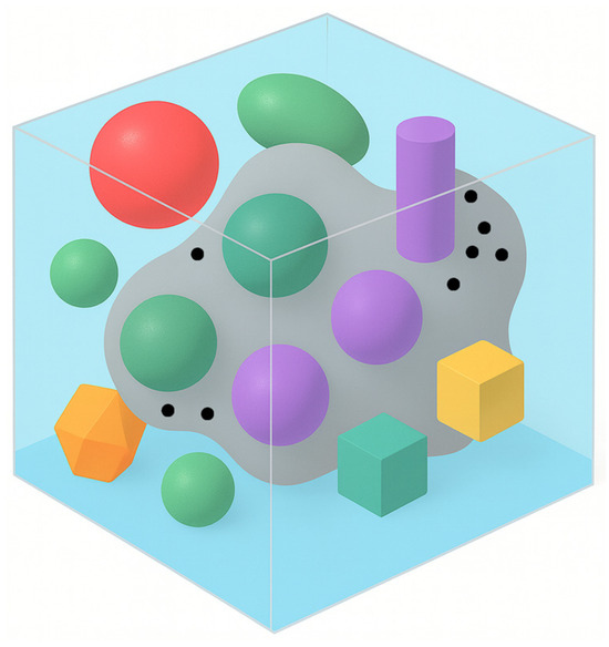
Figure 1.
Sample element of a multiphase body with a randomly nonhomogeneous structure and internal mass sources.
We assume that internal deterministic mass sources act within the body ( is the running point vector, t represents time), meaning the source intensity may be time-dependent, constant, or confined to a specified subregion of the body. In Figure 1, point sources are indicated by black dots, and the subregion in which sources act is shaded grey. The coordinates of each source are assumed to be known.
The mass concentrations of impurity (, where is the mass of the -th component within a unit volume, is the total mass of substance occupying that unit volume) in the matrix (domain ) and in the inclusions (domains , ) in the presence of internal mass sources, are described by the diffusion equations [38,39], written separately for each phase
Here is the matter density in the random subregion ; is the impurity kinetic transfer coefficient in .
We assume the inclusions are entirely contained within the body, i.e., the matrix occupies the external boundary of the body. The following initial and boundary conditions are imposed,
where denotes the outer boundary of the body.
On the region interfaces (), the conditions of equality of the chemical potentials and the equality of diffusive fluxes of the impurity species hold [40,41]
where the coefficients and are defined on open sets, namely
Here, denotes the domain of continuity of the function; is the boundary of -th simply connected subdomain of the -th phase and is the global phase-contact boundary, composed of the interfaces of the simply connected subdomains, with the number of simply connected subdomains in phase . Across the contact boundary, , the coefficients exhibit jumps, and , respectively.
On general thermodynamic grounds, the chemical potential depends logarithmically on concentration [40,42]
where is the chemical potential of the pure substance in the state characterized by absolute temperature and pressure ; is a coefficient involving the universal gas constant and the atomic mass of the impurity particles; and is the activity coefficient, which for a multiphase body can be expressed as
Substituting expression (4) into (3) with (5) considered yields the non-ideal contact conditions for the impurity concentration in the form
where .
In this formulation, the random quantities are the contact interfaces—i.e., the boundaries of the subdomains , which lie inside the body—thereby rendering the concentration field of the diffusing particles stochastic.
3. Mass Transfer Equation for the Entire Body
We reduce the contact diffusion problem (1), (6) and (7) to a mass-transfer equation for the body as a whole. To this end, introduce a random function of the spatial coordinate , that describes the concentration throughout the entire body, namely
We also introduce a random operator , i.e., the “structure function”, defined by
which satisfies the material continuity (partition-of-unity) condition
Then the diffusion coefficient , , and the density can be represented via the random structure function (8) in the form
We take into account that
(a) The function and its gradient have first kind (jump) discontinuities on the contact interfaces (conditions (6), (7));
(b) For the body as a whole, the mass balance equation holds
where is the impurity flux and
the coefficient is piecewise constant, has first-kind discontinuities at the contact interfaces, and is constant within each phase; therefore, the action of the nabla operator on can be written as
where is the position vector of points on the interface ; denotes the jump of a function across the interface ; is the Dirac delta function.
Note that the jump is, in general, a vector quantity and takes different values for different position vectors .
Equation (11) can be written in the form [43]
Here, we used the fact that the concentration is piecewise continuous in time together with its first time derivative. We also assume that the domains of continuity of the kinetic transport coefficient and of the concentration function coincide, hence .
Using the material continuity (partition-of-unity) condition (9) and the representations (10), the diffusion equation for the entire body can be written as
Adding and subtracting in Equation (12) the deterministic operator with coefficients characteristic of the matrix, we obtain
where is written as follows
Thus, we arrive at a stochastic mass-transfer differential equation for impurity in a multiphase medium with randomly distributed inclusions, given by (13) with the random operator (14).
4. Integro-Differential Mass-Transfer Equation—Neumann Series
Interpreting the right-hand side of Equation (13) as source terms for mass transfer in the randomly inhomogeneous multiphase body, we write an integro-differential equation equivalent to the original contact boundary-value problem (1), (6) and (7) [41]
Here is the solution to the following homogeneous problem
is the Green’s function, i.e., the solution of the corresponding deterministic boundary-value problem with a point source, specifically
internal region of the body.
We seek the solution of the integro-differential Equation (15) by the method of successive approximations (simple iteration) in the form of a Neumann integral series.
As the zero-order approximation we choose the sum of the solution to the homogeneous boundary-value problem (16), (17) and the convolution of the Green’s function with the source. This yields the following recurrence relations
Note that since is a continuously differentiable function, the application of the operator on it can be written as
In the constructed sequence of functions , , …, , … the general term can be written as
Here denotes the difference between -th and -th terms of the sequence, namely
We associate with this sequence the series:
which is an (integral) Neumann series.
Proposition 1.
If the diffusion coefficients () and densities () are bounded functions and , and the body has finite volume , then the Neumann integral series (21) is absolutely and uniformly convergent.
Proof.
The solution of the integro-differential Equation (15) is constructed by the method of successive approximations, taking as the zero-order approximation (19) the solution of the homogeneous initial boundary-value problem (16), (17) and introducing a parameter . Then the -th iteration takes the form
Let us denote
and
Now express the concentration field using the notations (23)
where is the operator notation for the double integral over the domain . This leads us to
where , which we verify by mathematical induction.
Setting and using the zero-order approximation yields Formula (22), so the assertion for the first iterate holds. Suppose the statement (24) is valid for -th iterate; we now show that the corresponding statement for the -th iterate also holds. Hence,
We next show that, for bounded , and , all iterates are continuous and bounded in the domain :
where , , .
From estimate (25), it follows that the series (21) is dominated termwise by the numerical series
which converges absolutely for
Accordingly, under condition (26), the Neumann series (21) is absolutely and uniformly convergent. Therefore, the successive approximations in (24) converge uniformly to the sought function as .
This completes the proof. □
The convergence of the Neumann series (21) requires that the number of inclusions () in phase j be specified or at least be finite. By contrast, the coefficients () that determine the jump of the concentration across random interphase interfaces may take arbitrary values. Likewise, no condition on characteristic inclusion sizes is needed.
We also note that, in the steady-state limit , the Neumann series diverges under the above (relatively mild) assumptions, since the domain of convergence in the stationary problem is substantially smaller than in the nonstationary case [44].
The first two terms of the Neumann series correspond to the concentration field in a homogeneous body with the characteristics of the base phase under the action of internal mass sources of power . The next two terms represent the sum of single-inclusion perturbations (placing one inclusion at a time). The third pair accounts for the pairwise influence of inclusions in the presence of internal sources, and so on. Jumps of the diffusion coefficient and the density of the body across interphase interfaces are incorporated via the operator .
For brevity, let us denote the second term in (21) by :
Then the Neumann series (21) can be written as
Note that the first two terms of (27) are deterministic, whereas all higher-order terms are random.
5. Feynman Diagrams for Mass Transfer in a Stochastically Inhomogeneous Multiphase Body
The Neumann series (21) is the expansion of the random concentration field with the perturbations accounting for the inclusions exhibiting characteristics different from the matrix. Before analyzing the Neumann series, we first fix a diagrammatic dictionary for the objects entering (21); throughout, we use the standard conventions of [43], see also [31].
Let a straight-line segment whose endpoints are assigned the coordinates and correspond to the Green’s function [37]:

Operator will correspond to the vertical segment with dots at its ends:

Random concentration field function and the homogenous concentration under the action of internal mass sources will be associated with the checkmark symbol and the wavy line correspondingly:

A diagram vertex is any point , , at which the lines representing , , and meet. The integration is performed over the internal vertex coordinates. The number of internal vertices equals the order of the diagram. With this dictionary in place, each term of (27) corresponds to a unique Feynman diagram. The first two terms on the right-hand side of (27) are represented by

In general, the -th order contributions to the Neumann series for have the structure (20): they contain Green-function lines and internal vertices , …, , and they always end with the wavy line corresponding to [37]

Accordingly, the series (27) admits the following graphical representation:

Let denote averaging over the ensemble of phase configurations. Averaging the random concentration field (27), (28) then yields
Under this framework, the first approximation is a linear functional of the fluctuations of the transport parameters , . Consequently, every moment of the field can be expressed linearly via the moments and of the same order.
Retaining only the first four terms of the Neumann series (29), i.e., the Born approximation [45] for the averaged concentration, one obtains the following expression for the averaged concentration field
In this setting, .
By definition, the (auto)correlation function and the variance of the of the random concentration field [46] are
The complete statistical properties of the field are encoded in cumulant functions of all orders. In the diagrammatic language, we associate cumulants with the dashed lines where the order of a cumulant matches the order of the associated diagram:

Since the concentration field is deterministic with respect to time, the time variable appears in cumulant functions merely as a parameter.
In general, the moments of the operator , which contains the fluctuations of and , can be written as [46]
or, equivalently, in the following diagrammatic form:

Observe first that expression (31), (32) expands into a sum of terms where the arguments , , …, are combined in all admissible ways. Consequently, upon averaging over the ensemble of phases, one obtains exactly diagrams of order , with the vertices interconnected in every possible manner.
Because we integrate over the coordinates of the internal vertices , the analytic expression represented by any given diagram carries no explicit dependence on those internal coordinates. For this reason, we henceforth omit internal-vertex labels from the drawings.
We now introduce a dedicated graphical symbol for the averaged concentration field in a non-homogeneous medium,


Here, terms up to and including third order (diagrams with three vertices) are shown.
For example, diagram 6 of series (33), namely

The correspondence between Feynman diagrams and analytic expressions is one-to-one, and a physical reading of the diagrams is given in [31].
Several diagrams entering (33) contain lower-order subdiagrams; we exploit this to streamline the analytic notation.
Representing the solution of the boundary-value problem (13), (2) by the diagram set (33) makes it possible to rearrange the Neumann series using certain topological features of the contributing diagrams.
In fact, the sum of (33) can be rewritten as the sum over a certain infinite subsequence of the same series. To this end, we adopt the classification from [47] to categorize the diagrams in (33) into weakly and strongly connected. A diagram is weakly connected if it can be split into two separate diagrams by cutting a single line . In (33) diagrams 3 and 5–7 are weakly connected, whereas 1, 2, 4, 8, and 9 are strongly connected. Diagrams produced by cutting a line may themselves be either strongly or weakly connected. Whenever “secondary” diagrams are weakly connected, we continue the splitting. Iterating this process yields a collection of strongly connected components. The connectivity index of the original diagram is thus defined as the number of strongly connected components obtained in this way. In (33), diagrams 3, 6, and 7 have connectivity index 2, diagram 5 has index 3, and every strongly connected diagram is assigned index 1.
From the series (33), extract all strongly connected diagrams. Because every such diagram starts with -line and with the wavy line , the sum of all strongly connected diagrams can be written as

In analytic form this becomes
where is the mass-operator kernel
with the following graphical representation

Next, let us consider all strongly connected diagrams with connectivity index 2. Each of them has the structure

 and
and  are arbitrary diagrams taken from the right-hand side of (36).
Since the construction of the series (29), (33) enumerates all pairwise connections of internal vertices, the sum of all terms of the form (37) equals

 denotes the complete sum (36).
By the same reasoning, the sum of all diagrams with connectivity index 3 has the form


Let us verify that the series (38) satisfies the equation

Although is formally introduced as an operator, in the present context it has a clear physical meaning. The kernel represents the cumulative influence of random phase interfaces on impurity transport. In diagrammatic terms, it corresponds to the sum of all strongly connected diagrams and thus encapsulates how multiple phase-boundary interactions in the stochastic multiphase structure renormalize the bare diffusion operator and modify the effective transport of the averaged concentration field.
To solve Equations (39) and (40), we employ the method of successive iteration. Substituting expression [48]. Substituting expression (39) and (40) into the right-hand side of the same equation yields, for the averaged concentration field we obtain

Substituting the right-hand side of (39), (40) into the expression obtained above, we get

Repeating this substitution iteratively generates the series (38). In analytic terms, applying the same procedure yields the expansion
Viewing as given, Equations (39) and (40) is an integral equation for , which we can find explicit solutions for in some cases. In that event one obtains an expression for the averaged concentration in terms of the mass-operator kernel ; equivalently, the sum of series (29), (33) can be written through (34), (35), which represents a particular subsequence of the same series.
In general, the operator, or, in some cases, the function, is not known precisely. A practical route is to approximate it by the sum of the first few terms of series (38), (41). For example, in the Bourret approximation [47] one has

Using the form of the operator from (14), the expression for under non-ideal interfacial (contact) conditions on the concentration can be written as
We denote graphically the Bourret approximation for the averaged field by

Alternatively, by replacing with the diagram (42) in expression (38), (41) we obtain the following representation of :
 or, in analytic form,
Thus, both analytic and diagrammatic expressions have been derived for the concentration field averaged over the ensemble of phase configurations, within the Bourret approximation.
6. Equation for the Averaged Concentration Field in a Multiphase Randomly Inhomogeneous Medium with Internal Sources
We now derive the equation whose solution is the averaged concentration field . Apply the diffusion operator with base-phase characteristics to the Dyson Equations (39) and (40). This gives
Using relations (16) and (18), Equation (45) can be rewritten as
and, upon integration, we obtain
In the Bourret approximation, using (42), the resulting equation reduces to
If the averaged field and its first derivatives are continuous in all spatial coordinates, then
Assume further that the phases are uniformly distributed throughout the body. Then Equation (48) takes the form
In the case of a two-phase body, Equation (49) is equivalent to
whereas for a three-phase body we have
If we adopt the following approximation for the mass-operator kernel

Then Equation (46) becomes
Let us compare the equations for under the action of internal mass sources obtained with the kernel approximations (42) and (51), i.e., Equations (47) and (52). Note that, under the approximation the averaged concentration field satisfies an integro-differential rather than a purely differential equation. Physically, this reflects nonlocality, namely at a point depends on the surrounding inhomogeneities.
7. Influence of Internal Mass Sources on the Averaged Impurity Concentration in a Two-Phase Randomly Inhomogeneous Layer
To investigate how internal sources affect the behavior of the averaged concentration field, we consider impurity diffusion in a two-phase, randomly inhomogeneous layer, deduced in the Bourret approximation. The phases are assumed to be distributed uniformly within the body.
For a layer of thickness with internal sources of power the diffusion process is governed by the initial boundary value problem based on Equation (50). In one spatial dimension this reads
subject to a zero initial condition and prescribed constant boundary concentrations at the top and bottom faces
We now consider several types of source terms .
7.1. Single Point Mass Source
Let a point source of power act at , :
We seek the solution of (53), (54), (55) by reducing to homogeneous boundary conditions, applying a finite sine transform in the spatial variable, and a Laplace transform in time. The result is obtained in the form
where
All numerical calculations here and below are carried out in dimensionless variables [49] , , i.e., time is normalized by matrix characteristics. The baseline problem parameters are , , , , , , .
Representative distributions of the averaged impurity concentration in the Bourret approximation for various internal source types are shown in Figure 2, Figure 3, Figure 4, Figure 5, Figure 6, Figure 7 and Figure 8. The series occurring in the formulas for were summed to a tolerance of .
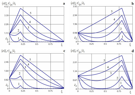
Figure 2.
Charts of the averaged concentration under the action of a point source for , (a), , (b), , (c), , (d) at different moments of dimensionless time.
Modeling software was implemented in C# using Visual Studio 2022 Community Edition. Visualizations were rendered using Plotly.Net 5.1.0 and ScottPlot 4.1.68. All computations ran on a 64-bit Windows 11 Pro system with an Intel Core i7-1065G7 CPU and 16.0 GB RAM.
Figure 2 shows the distributions of the function under the action of a point source of power evaluated at times 0.001, 0.01, 0.05, 0.1, 0.5 (curves 1–5, respectively). Figure 2a corresponds to a source located at 0.2, Figure 2b to point 0.8 for . Figure 2c displays the influence of a source located at 0.2, and Figure 2d at 0.8 for . The solutions were computed from Formula (56).
Note that the action of an internal point source increases the impurity concentration throughout the entire layer. A larger source power yields larger values of . A local maximum of the averaged concentration is observed at small times, and a global maximum at large times, in the vicinity of the point source (Figure 2). In this neighborhood, the concentration function loses smoothness. For small times, the concentration decreases away from the upper surface of the layer; the local minimum is located closer to the source point, but over time the concentration increases and the local minimum shifts toward the upper boundary of the layer (curves 1, 2 in Figure 2a,c and curves 1–4 in Figure 2b,d). For larger times, the function increases from the surface , attaining its maximum near the point source (curves 3–5 in Figure 2a,c, and curves 5 in Figure 2b,d), after which the concentration decreases toward the surface .
Note also that an increase in the diffusion coefficient leads to a decrease in the concentration throughout the body (Figure 2a–d). For example,
7.2. Finite Number of Deterministic Mass Point Sources
Consider the case of point mass sources
where is the power of -th source.
The solution of the boundary-value problem (53), (54), (57) has the form
Figure 3 shows graphs of the averaged concentration of migrating particles for a finite number of point sources acting inside the layer at times 0.001, 0.01, 0.05, 0.1, 0.5 (curves 1–5). Figure 3a illustrates the distributions of , computed for nine sources located at {0.1, 0.2, 0.3, 0.4, 0.5, 0.6, 0.7, 0.8, 0.9} with equal power , . Figure 3b–d are plotted for four sources of equal power (). In Figure 3b, the sources are placed closer to the upper boundary at {0.1, 0.2, 0.3, 0.4}, in Figure 3c they are near the center of the strip {0.35, 0.45, 0.55, 0.65}, in Figure 3d they are in the lower part of the strip {0.6, 0.7, 0.8, 0.9}. Figure 3e–g show graphs of the averaged concentration for four sources located at {0.1, 0.2, 0.8, 0.9}. In Figure 3e, the sources have equal power (), in Figure 3f, there is a dominant source of power at 0.1, in Figure 3g of power at 0.9. Figure 3h shows concentration distributions for nine sources at {0.1, 0.2, 0.3, 0.4, 0.5, 0.6, 0.7, 0.8, 0.9} with one dominant source at at point , while the other sources have equal power , .


Figure 3.
Graphs of the averaged impurity concentration at various dimensionless times under the action of several point sources located inside the layer (panels (a,c)) and near the body surfaces (panels (b,d–h)).
Figure 3.
Graphs of the averaged impurity concentration at various dimensionless times under the action of several point sources located inside the layer (panels (a,c)) and near the body surfaces (panels (b,d–h)).
The action of point sources in the strip increases the impurity concentration throughout the entire body, with the largest increase in the neighborhood of the point sources. As in the single-source case, for small times the averaged concentration exhibits local maxima in small neighborhoods of the source locations (curves 1–3 in Figure 3a–h), and the function is not smooth. As time increases, these local maxima are leveled out and the function approaches a piecewise-linear profile. In all cases considered, the global maximum of the concentration is attained near one of the sources: near a middle source when the sources have equal power (Figure 3a–d), or near the dominant source when present (Figure 3f–h). Note that increasing the diffusion coefficient in the inclusions decreases the averaged concentration throughout the body, while the qualitative behavior of the function remains unchanged. Increasing the power of one source, or the number of sources, increases the concentration values throughout the body, the largest values occur over the interval where the internal point sources act. Also note that the effect of each individual source is pronounced at small times (curves 1–3 in Figure 3a–g). In contrast, at large times the impurity concentration spreads over the body and the sources act as an integral whole. In all cases, the steady regime of is reached at time .
7.3. Constant Power Source Acting Throughout the Body
Consider the following rule for the acting source
where is the power of the source.
The solution of the boundary-value problem (53), (54), (59) has the form
Figure 4 presents plots of the averaged concentration under a source of constant power acting throughout the entire body (60). Figure 4a is computed for source power. , and Figure 4b for . Curves 1–5 correspond to the next values of dimensionless time 0.001, 0.01, 0.05, 0.1, 0.5.


Figure 4.
Averaged impurity concentration at various dimensionless times under the influence of the constant-power source acting throughout the body (panel (a)) and (panel (b)).
Figure 4.
Averaged impurity concentration at various dimensionless times under the influence of the constant-power source acting throughout the body (panel (a)) and (panel (b)).
Note that the presence of a constant-power source acting in the whole body increases the impurity concentration at both small and large dimensionless times. Moreover, the larger the source power, the larger the values of (Figure 4a,b). For small times or for a small mass source power (curves 1, 2 in Figure 4a and curves 1–4 in Figure 4b) the behavior of is similar to that in the absence of internal sources. The concentration function also remains smooth over the entire interval. For small times, the concentration decreases away from the boundary (curves 1–3 in Figure 4a and curves 1–4 in Figure 4b). As diffusion proceeds, the concentration grows and becomes an increasing function in a neighborhood of the upper boundary (curves 4, 5 in Figure 4a and curve 5 in Figure 4b). In addition, a constant source of substantial power leads to the appearance of a global maximum that grows with time and shifts deeper into the body (curves 4 and 5 in Figure 4a). Note that in the steady regime, the function is convex (curve 5 in Figure 4). The time to reach the steady state of the averaged concentration is the same for different values of , namely .
7.4. Constant Power Source Acting on an Interval
Consider the interval and the following law for the source action
The solution of the boundary-value problem (53), (54), (61) has the form
Figure 5 shows distributions of the averaged concentration of the migrating impurity substance in a two-phase body in the presence of a constant source acting on a prescribed interval, for power (Figure 5a) and (Figure 5b–d). Figure 5a depicts function for the source action interval [0.4, 0.6], Figure 5b—for [0.1, 0.3]; Figure 5c—for [0.7, 0.9] and Figure 5d—for [0.3, 0.7]. Curves 1–5 correspond to the dimensionless times 0.001, 0.01, 0.05, 0.1, 0.5.


Figure 5.
Averaged impurity concentration at various dimensionless times under a constant-power source acting on an interval located inside the body (panels (a,d)), near the upper boundary (panel (b)), and near the lower boundary (panel (c)).
Figure 5.
Averaged impurity concentration at various dimensionless times under a constant-power source acting on an interval located inside the body (panels (a,d)), near the upper boundary (panel (b)), and near the lower boundary (panel (c)).
As with the source types considered above, the presence of a constant source acting on a finite interval increases the concentration throughout the body, most strongly in the vicinity of that interval; this growth occurs both at small and at large times (Figure 5). In this case as well, the function remains smooth. For small and intermediate times, the concentration decreases away from the boundary , reaches a local minimum in the interior, and then increases to a local maximum. This maximum increases with time and shifts toward the upper boundary of the layer (curves 2–4 in Figure 5a,c,d).
The time for the averaged concentration to reach the steady regime is for the source powers considered and for the various placements of the action interval. For times close to steady state, the rate of concentration growth throughout the body drops considerably.
7.5. Two Constant Power Sources Acting on Subintervals
Let two constant-power sources act on the subintervals and , . Consider the following
where is the Heaviside step function. The solution of the boundary-value problem (53), (54), (63) is found as follows
where , represent the power of the sources.
Figure 6 shows the behavior of the averaged concentration in a two-phase body in the presence of two constant mass sources acting on different prescribed intervals (64), for large powers (Figure 6a,c,d) and for small powers (Figure 6b). Figure 6a–d display the distributions of under sources acting on the intervals: Figure 6a,b— [0.1, 0.3] and [0.7, 0.9], Figure 6c— [0.35, 0.45] and [0.55, 0.65], Figure 6d— [0.5, 0.55], [0.7, 0.95]. Curves 1–5 correspond to the dimensionless times 0.001, 0.01, 0.05, 0.1, 0.5.


Figure 6.
Averaged impurity concentration at various dimensionless times under two constant-power sources acting on prescribed intervals [0.1, 0.3] and [0.7, 0.9] (panels (a,b)), [0.35, 0.45] and [0.55, 0.65] (panel (c)), [0.5, 0.55] and [0.7, 0.95] (panel (d)).
Figure 6.
Averaged impurity concentration at various dimensionless times under two constant-power sources acting on prescribed intervals [0.1, 0.3] and [0.7, 0.9] (panels (a,b)), [0.35, 0.45] and [0.55, 0.65] (panel (c)), [0.5, 0.55] and [0.7, 0.95] (panel (d)).
Note that the action of two constant sources on prescribed intervals increases the concentration throughout the entire body, both at small and at large times (Figure 6). The influence of this source type is most pronounced at intermediate diffusion times (curves 2–4, Figure 6a). Increasing the power of one or both sources substantially raises the averaged concentration at intermediate and large times (Figure 6a,b); for example, increasing the powers , by a factor of 5 leads to a 1.8-fold increase of at the point , with a global maximum forming at (curve 5, Figure 6a). For small times, the mass-transfer process proceeds similarly for different source powers, and the influence of the value , is minor (curve 1, Figure 6a,b). When the sources act on two separated intervals, the concentration decreases from the upper boundary of the body, increases in the neighborhood of the first source, then decreases again and increases near the second source, with a characteristic decline toward the lower boundary (Figure 6a,d). When the action intervals are adjacent (Figure 6c), the behavior of the concentration field is essentially the same as for a single constant source acting on the combined interval . In all cases, the function remains smooth.
7.6. Impulsive Sources Acting at Specified Times
Consider an impulsive source acting at times
The solution of the boundary-value problem (53), (54), (65) is obtained as
Figure 7 shows the behavior of the averaged concentration of impurity particles diffusing in a two-phase body in the presence of a source that acts instantaneously at specified dimensionless times throughout the entire body. Figure 8, Figure 9, Figure 10 and Figure 11 present surfaces (panels a), formed by the variation in concentration over time (ordinate) within the body region (abscissa), together with the corresponding contour plots of (panels b).
In Figure 7a and Figure 8, we show the effect of sources of equal power at four instants (). In Figure 7a–d, curves 1–5 correspond to the distributions of the averaged concentration at times 0.001 (the internal sources have not yet acted), 0.01 (the source acted at the first instant 0.005), 0.05 (the source acted at 2 times 0.005 and 0.03), 0.1 ( 0.005, 0.03, 0.08), 0.5 ( 0.005, 0.03, 0.08, 0.4).
Figure 7b and Figure 9 illustrate the distributions for the same set of times but with a larger source power ,. Figure 7c and Figure 10 show the graphs of when there is a dominant-power impulse at the first instant , namely {1, 0.3, 0.3, 0.3}; Figure 7d and Figure 11 correspond to a dominant impulse at the last instant , namely {0.3, 0.3, 0.3, 1}.


Figure 7.
Plots of the averaged impurity concentration at different times under an impulsive mass source of equal small (panel (a)) and large (panel (b)) powers at all instants, and with a dominant-power impulse at the first (panel (c)) and last (panel (d)) instants.
Figure 7.
Plots of the averaged impurity concentration at different times under an impulsive mass source of equal small (panel (a)) and large (panel (b)) powers at all instants, and with a dominant-power impulse at the first (panel (c)) and last (panel (d)) instants.
Figure 8.
Three-dimensional (panel (a)) and two-dimensional (panel (b)) plots of the averaged impurity concentration for four impulses of small power at respective times.
Figure 8.
Three-dimensional (panel (a)) and two-dimensional (panel (b)) plots of the averaged impurity concentration for four impulses of small power at respective times.

Figure 9.
Three-dimensional (panel (a)) and two-dimensional (panel (b)) plots of the averaged impurity concentration for four impulses of large power at respective times.
Figure 9.
Three-dimensional (panel (a)) and two-dimensional (panel (b)) plots of the averaged impurity concentration for four impulses of large power at respective times.


Figure 10.
Three-dimensional (panel (a)) and two-dimensional (panel (b)) plots of the averaged impurity concentration for four impulses with powers .
Figure 10.
Three-dimensional (panel (a)) and two-dimensional (panel (b)) plots of the averaged impurity concentration for four impulses with powers .


Figure 11.
Three-dimensional (panel (a)) and two-dimensional (panel (b)) plots of the averaged impurity concentration for four impulses with powers .
Figure 11.
Three-dimensional (panel (a)) and two-dimensional (panel (b)) plots of the averaged impurity concentration for four impulses with powers .

Note that the action of a time-instantaneous (impulsive) point mass source substantially increases the impurity concentration in the body after each impulse. The increase in grows with the source power (curves 1–4, in Figure 7a,b). For small times, the averaged concentration function is monotonically decreasing (curves 1, Figure 7a–d). Subsequently, the concentration increases throughout the body (curves 2, Figure 7) and a maximum forms in the upper half of the layer (curves 3, 4, Figure 7). Thereafter, the values decrease until the steady regime is reached (curves 5, Figure 7a–c). If a dominant-power point source acts at the first instant then the values of the averaged concentration increase by up to a factor of two compared with equal-power impulses (curves 3, Figure 7a,c). For example,
If the dominant-power source acts at the last instant , then at time we have
Also, observe that the growth of in neighborhoods of the impulse times is step-like (Figure 8, Figure 9, Figure 10 and Figure 11). The function maximum is attained exactly at the instant an impulse acts. The magnitudes of the local and global maxima over time depend on the source powers and on the concentration level prior to their action (Figure 9 and Figure 11). The subsequent decay to lower concentration levels is gradual. If the interval between successive impulses is sufficiently large, then may decrease to the level corresponding to the absence of sources (Figure 10 and Figure 11). Compared with the other source types, the time to reach the steady regime is longer in this case.
7.7. Constant Power Sources Acting over Time Interval
Let a constant-power source act over the time interval
The solution of the boundary-value problem (53), (54), (66) has the form
Figure 12, Figure 13 and Figure 14 illustrate the behavior of the averaged concentration of impurity particles diffusing in a two-phase layer in the presence of a source that acts over a prescribed time interval throughout the entire body. Here, the source power is . In Figure 12a and Figure 13, we show the effect on of such a source acting on the time interval , in Figure 12b and Figure 14—on the longer interval . Curves 1–5 in Figure 12 correspond to the dimensionless times 0.001, 0.01, 0.05, 0.1, 0.5. Figure 13 and Figure 14 present surface plots formed by the variation in concentration in time (ordinate) along the body (abscissa) in the space.
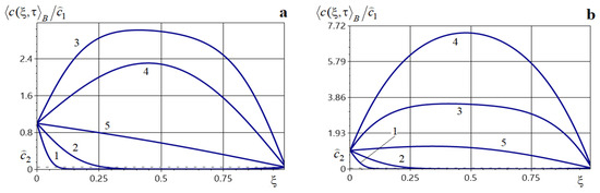
Figure 12.
Plots of the averaged concentration at various dimensionless times under a source acting throughout the body, over a short time interval (panel (a)) and a long time interval (panel (b)).
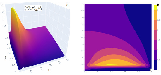
Figure 13.
Three-dimensional (panel (a)) and two-dimensional (panel (b)) plots of the averaged impurity concentration under a constant power source acting over the short time interval .
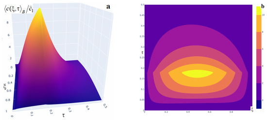
Figure 14.
Three-dimensional (panel (a)) and two-dimensional (panel (b)) plots of the averaged impurity concentration under a constant power source acting over a long time interval .
A marked increase in impurity concentration is observed throughout the entire time interval during which the internal constant source acts, and even after its action ceases (Figure 12). At the beginning of the interval , the concentration values are small (curves 1 and 2 in Figure 12). The concentration function then increases substantially and this growth continues as long as the source is active (curve 3, Figure 12a and curves 3, 4, Figure 12b). In this case, function attains its maximum at the final instant of the Interval (curve 3 in Figure 12a and curve 4 in Figure 12b). For example, the maximum of the averaged concentration for a constant power source acting on is reached at time at point and equals (Figure 13). Note that the values of the function are larger the longer the source acts over a finite time interval. For instance, doubling the interval length leads to a twofold increase of at the point , while increasing the interval by a factor of 5.5 raises the concentration by a factor of 1.37 at the same point. The twofold increase observed when extending the interval from to is due to the observation time being distant from the source action in the first case, and coming immediately after the source ceases in the second case. Also note that, once the source is turned off, the concentration begins to decrease until the steady regime is reached at time (curve 5, Figure 12a).
We also note that a source acting over time intervals causes a rapid (though not instantaneous) increase in concentration in time. Likewise, after the source action ends, the subsequent decrease is also rapid, but slower than the preceding growth.
7.8. Comparative Analysis of the Averaged Concentration Distributions with and Without Internal Mass Sources
We investigate the influence of sources on the behavior of the averaged concentration by comparing it with the distribution of the function in the absence of internal sources. In the latter case, the solution is described by formula [35]
Figure 15 illustrates the distributions of at the dimensionless times 0.05, 0.1, 0.3 (curves 1–3, respectively) for various types of sources (curves a, solid lines) and in their absence (curves b, dashed lines). Specifically, Figure 15a is plotted for a point source of power , located at . Figure 10b corresponds to nine point sources of equal power , located at points with coordinates (). Figure 15c shows , when a source of power acts over the spatial interval . Figure 15d is plotted for a source acting over the time interval with the power . The computations were performed using Formulas (56), (58), (62), (67) and (68).
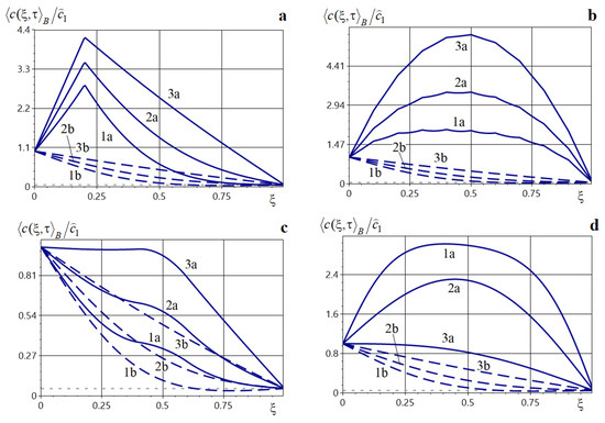
Figure 15.
Distributions of the averaged concentration with and without sources acting within the body for a single point source (Panel (a)), a set of point sources (Panel (b)), a source acting on a spatial interval (Panel (c)), and a source acting on a temporal interval (Panel (d)).
Note that the presence of internal mass sources not only substantially increases the averaged concentration within the body, but also changes the qualitative behavior of the function (Figure 15a–d).
7.9. Averaged Hydrogen-Concentration Field in the Composite Cu-Fe Structure
Consider the problem of hydrogen migration in a composite taking copper as the matrix (base) phase. The hydrogen diffusion coefficients were taken as follows [50,51]: in copper , in iron , the densities are for copper, and for iron. Hence, we obtain and .
Figure 16 illustrates the behavior of the averaged hydrogen concentration field at various dimensionless times for (Figure 16a) and (Figure 16b) in the composite under a point source of power located at . Curves 1–5 correspond to the dimensionless times .
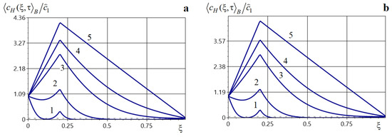
Figure 16.
Distributions of the averaged concentration of H in structure at different times for (Panel (a)) and (Panel (b)) for the point mass source of power acting at .
Note that the larger the copper volume fraction, the more rapidly the averaged hydrogen concentration approaches a steady regime (Figure 16). The presence of a point source results in a local maximum at the source location (curves 1, Figure 8a,b), which then becomes a global maximum (curves 2–5, Figure 16a,b).
Figure 17 shows the behavior of the ensemble-averaged hydrogen concentration field at various dimensionless times for (Figure 17a) and (Figure 17b) in the composite under a domain-wide constant-power source with acting over the time interval . Curves 1–5 correspond to dimensionless times .
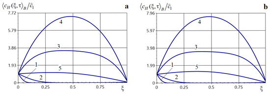
Figure 17.
Distributions of the averaged concentration of H in structure at different times for (Panel (a)) and (Panel (b)) for the constant mass source of power acting over period.
As time increases, the hydrogen concentration in the composite grows substantially throughout the body (curves 1–3, Figure 17), and a maximum , forms. It then increases in magnitude and shifts towards the center of the body as increases (curves 4 and 5 in Figure 17).
The obtained results provide a theoretical framework for modelling and optimisation of diffusion-driven processes in complex media. Although detailed engineering aspects are beyond the scope of this paper, the presented approach can be used as a mathematical basis for studying transport phenomena in multiphase materials or biological tissues where random inhomogeneities play a key role.
8. Conclusions
In this work, we have developed and analyzed a mathematical model for impurity diffusion in randomly inhomogeneous multiphase media with deterministic internal mass sources. Using a diagrammatic–operator technique based on Feynman diagrams, we derived the Dyson equation for the averaged concentration field and established convergence of the associated Neumann series. This provides a rigorous theoretical framework for studying transport in complex composite systems and a basis for further extensions.
Thus, we have investigated the concentration of an impurity migrating in a multiphase, stochastically inhomogeneous body under deterministic internal mass sources. Based on mass-balance equations for each phase, with non-ideal contact conditions on random interphase interfaces, we formulated a contact initial boundary-value problem for the entire body.
The original problem is shown to be equivalent to an integro-differential equation with a random kernel. In this equation, the internal mass sources contribute an additional integral term. Its solution was obtained by successive approximations as a Neumann series, and its absolute and uniform convergence was proven. The random concentration field was then averaged over the ensemble of phase configurations.
To analyze the structure of the averaged series, we employed the Feynman-diagram technique:
- A classification was proposed and the diagrams were grouped into strongly and weakly connected classes;
- The mass-operator kernel was obtained as the sum of all strongly connected diagrams, enabling the derivation of the Dyson equation for the averaged concentration field;
- It was shown that the averaged Neumann series solves the Dyson equation.
Throughout the mathematical modeling of impurity diffusion in a multiphase, randomly inhomogeneous body, the contributions due to internal mass sources are retained at every stage. For uniformly distributed phases, mass-transfer equations were obtained for an N-phase body, in particular for two- and three-phase layers. In the Bourret approximation, boundary-value problems were solved for various source types—spatially distributed: a single point source, a collection of point sources, and a source acting on one or two intervals; and temporally distributed: impulsive at discrete times and of constant power acting over a prescribed time interval. The present study considers deterministic internal sources, which is a principal feature of the model. The extension to stochastic sources in randomly inhomogeneous media is planned as a separate investigation.
It was shown that for the impulsive point source, the averaged concentration exhibits a step-like increase near the impulse times; local maxima occur at the instants of source action, and the global maximum occurs at the time of the dominant-power impulse.
The proposed approach to modeling mass transport in randomly inhomogeneous bodies offers opportunities for analyzing the correlation characteristics of stochastic fields and for constructing a nonlocal equation for the associated coherence function; it is also amenable to extensions to irregular impulsive sources or sources arising from sorption processes and chemical reactions. In future work, we should also investigate the ensemble-averaged impurity concentration field under sources that operate at specific instants or over certain time intervals and are point-like in space.
Thus, incorporating internal mass sources into the mathematical model of a stochastically inhomogeneous medium substantially broadens the applicability of the diagrammatic–operator method and provides a foundation for further refinement of transport models in complex and composite stochastic systems.
Author Contributions
Conceptualization, P.P. and O.C.; methodology, P.P. and Y.C.; software, Y.C.; validation, P.P., O.C. and M.V.; investigation, P.P. and O.C.; data curation, Y.C.; writing—original draft preparation, O.C. and Y.C.; writing—review and editing, P.P. and M.V.; visualization, Y.C.; supervision, P.P.; project administration, P.P. and O.C.; funding acquisition, P.P., O.C. and M.V. All authors have read and agreed to the published version of the manuscript.
Funding
This research was funded by the Ministry of Education and Science of Ukraine, as part of the state budget research project № DR 0123U101691.
Data Availability Statement
The original contributions presented in this study are included in the article. Further inquiries can be directed to the corresponding author.
Conflicts of Interest
The authors declare no conflicts of interest. The funders had no role in the design of the study; in the collection, analyses, or interpretation of data; in the writing of the manuscript; or in the decision to publish the results.
References
- Dahlkemper, M.N.; Klein, P.; Müller, A.; Schmeling, S.M.; Wiener, J. Opportunities and challenges of using Feynman diagrams with upper secondary students. Physics 2022, 4, 1331–1347. [Google Scholar] [CrossRef]
- Kozik, E. Combinatorial summation of Feynman diagrams. Nat. Commun. 2024, 15, 7916. [Google Scholar] [CrossRef] [PubMed]
- Budzik, K.; Gaiotto, D.; Kulp, J.; Wu, J.; Yu, M. Feynman diagrams in four-dimensional holomorphic theories and the operatope. J. High Energy Phys. 2023, 7, 127. [Google Scholar] [CrossRef]
- Sberveglieri, G.; Spada, G. Phi4tools: Compilation of Feynman diagrams for Landau–Ginzburg–Wilson theories. J. High Energy Phys. 2024, 5, 73. [Google Scholar] [CrossRef]
- Aprile, F.; Olivucci, E. Multipoint fishnet Feynman diagrams: Sequential splitting. Phys. Rev. D 2023, 108, L121902. [Google Scholar] [CrossRef]
- Núñez Fernández, Y.; Jeannin, M.; Dumitrescu, P.T.; Kloss, T.; Kaye, J.; Parcollet, O.; Waintal, X. Learning Feynman diagrams with tensor trains. Phys. Rev. X 2022, 12, 041018. [Google Scholar] [CrossRef]
- Kugler, F.B. Counting Feynman diagrams via many-body relations. Phys. Rev. E 2018, 98, 023303. [Google Scholar] [CrossRef]
- De Doncker, E.; Yuasa, F.; Ishikawa, T. Numerical regularization for 4-loop self-energy Feynman diagrams. J. Phys. Conf. Ser. 2023, 2438, 012147. [Google Scholar] [CrossRef]
- Sidler, D.; Hamm, P. A Feynman diagram description of the 2D-Raman–THz response of amorphous ice. J. Chem. Phys. 2020, 153, 044502. [Google Scholar] [CrossRef]
- Rose, P.A.; Krich, J.J. Automatic Feynman diagram generation for nonlinear optical spectroscopies and application to fifth-order spectroscopy with pulse overlaps. J. Chem. Phys. 2021, 154, 034109. [Google Scholar] [CrossRef]
- Fukutake, N. Theoretical approach to resolution limit calculations in optical microscopy with the use of Feynman diagrams. In Frontiers in Optics/Laser Science, OSA Technical Digest; Optica Publishing Group: Washington, DC, USA, 2018; Paper JTu2A.41. [Google Scholar] [CrossRef]
- Fukutake, N. Comparison of image-formation properties of coherent nonlinear microscopy by means of double-sided Feynman diagrams. J. Opt. Soc. Am. B 2013, 30, 2665–2675. [Google Scholar] [CrossRef]
- Antczak, M.; Popenda, M.; Zok, T.; Zurkowski, M.; Adamiak, R.W.; Szachniuk, M. New algorithms to represent complex pseudoknotted RNA structures in dot–bracket notation. Bioinformatics 2017, 34, 1304–1312. [Google Scholar] [CrossRef]
- Başar, E. S-matrix and Feynman space–time diagrams to quantum brain approach: An extended proposal. NeuroQuantology 2009, 7, 30–45. [Google Scholar] [CrossRef][Green Version]
- Jovanovic, F.; Schinckus, C. Econophysics and Financial Economics: An Emerging Dialogue; Oxford University Press: Oxford, UK, 2017. [Google Scholar]
- Guevara, A.; Zhang, Y. Planar matrices and arrays of Feynman diagrams: Poles for higher k. Commun. Theor. Phys. 2024, 76, 045001. [Google Scholar] [CrossRef]
- Cachazo, F.; Guevara, A.; Umbert, B.; Zhang, Y. Planar matrices and arrays of Feynman diagrams. Commun. Theor. Phys. 2024, 76, 035002. [Google Scholar] [CrossRef]
- Clemente, G.; Crippa, A.; Jansen, K.; Ramírez-Uribe, S.; Rentería-Olivo, A.E.; Rodrigo, G.; Sborlini, G.F.R.; Vale Silva, L. Variational quantum eigensolver for causal loop Feynman diagrams and directed acyclic graphs. Phys. Rev. D 2023, 108, 096035. [Google Scholar] [CrossRef]
- Borges, F.; Cachazo, F. Generalized planar Feynman diagrams: Collections. J. High Energy Phys. 2020, 11, 164. [Google Scholar] [CrossRef]
- Castro, E.R.; Roditi, I. An exact solution method for the enumeration of connected Feynman diagrams. J. Phys. A Math. Theor. 2020, 53, 245203. [Google Scholar] [CrossRef]
- Acosta, J.F.; Andaluz, V.H.; Naranjo, M.X.; Molina, J.I.; Santana, A.G.; Topa, A.O.; Erazo, G. 3-D path planning using subatomic particles and Feynman diagrams. In Proceedings of the 2019 Third World Conference on Smart Trends in Systems Security and Sustainability (WorldS4), London, UK, 29–30 July 2019; pp. 368–375. [Google Scholar] [CrossRef]
- Derkachov, S.E.; Isaev, A.P.; Shumilov, L.A. Ladder and zig–zag Feynman diagrams, operator formalism and conformal triangles. J. High Energy Phys. 2023, 6, 59. [Google Scholar] [CrossRef]
- Ananthanarayan, B.; Das, A.B.; Wyler, D. Hopf algebra structure of the two-loop three-mass nonplanar Feynman diagram. Phys. Rev. D 2021, 104, 076002. [Google Scholar] [CrossRef]
- Shojaei-Fard, A. Graphons and renormalization of large Feynman diagrams. Opusc. Math. 2018, 38, 427–455. [Google Scholar] [CrossRef]
- Ablinger, J.; Blümlein, J.; Raab, C.G.; Schneider, C. Nested (inverse) binomial sums and new iterated integrals for massive Feynman diagrams. Proc. Sci. 2014, 211, 1–13. [Google Scholar] [CrossRef]
- Argeri, M.; Mastrolia, P. Feynman diagrams and differential equations. Int. J. Mod. Phys. A 2007, 22, 4375–4436. [Google Scholar] [CrossRef]
- Isaev, A.P. Operator approach to analytical evaluation of Feynman diagrams. Phys. At. Nucl. 2008, 71, 914–924. [Google Scholar] [CrossRef][Green Version]
- Barna, I.F.; Mátyás, L. Analytic solutions of the complex diffusion equation with aspects on quantum mechanics. Int. J. Mod. Phys. A 2025, 40, 2542009. [Google Scholar] [CrossRef]
- Nicholson, C. Diffusion and related transport mechanisms in brain tissue. Rep. Prog. Phys. 2001, 64, 815–884. [Google Scholar] [CrossRef]
- Patel, R.A.; Perko, J.; Jacques, D.; De Schutter, G.; Van Breugel, K.; Ye, G. A versatile pore-scale multicomponent reactive transport approach based on lattice Boltzmann method: Application to portlandite dissolution. Phys. Chem. Earth 2014, 70–71, 127–137. [Google Scholar] [CrossRef]
- Baqer, Y.; Chen, X. A review on reactive transport model and porosity evolution in the porous media. Environ. Sci. Pollut. Res. 2022, 29, 47873–47901. [Google Scholar] [CrossRef]
- Zhang, H.; Xiang, X.; Huang, B.; Wu, Z.; Chen, H. Static homotopy response analysis of structure with random variables of arbitrary distributions by minimizing stochastic residual error. Comput. Struct. 2023, 288, 107153. [Google Scholar] [CrossRef]
- Chen, W.; Hou, H.; Zhang, Y.; Liu, W.; Zhao, Y. Thermal and solute diffusion in α-Mg dendrite growth of Mg-5 wt.% Zn alloy: A phase-field study. J. Mater. Res. Technol. 2023, 24, 8401–8413. [Google Scholar] [CrossRef]
- Lanoiselée, Y.; Moutal, N.; Grebenkov, D.S. Diffusion-limited reactions in dynamic heterogeneous media. Nat. Commun. 2018, 9, 4398. [Google Scholar] [CrossRef]
- Pukach, P.; Chernukha, Y.; Chernukha, O.; Bilushchak, Y.; Vovk, M. Mathematical modeling of impurity diffusion processes in a multiphase randomly inhomogeneous body using Feynman diagrams. Symmetry 2025, 17, 920. [Google Scholar] [CrossRef]
- Stolk, P.A.; Gossmann, H.-J.; Eaglesham, D.J.; Jacobson, D.C.; Rafferty, C.S.; Gilmer, G.H.; Jaraíz, M.; Poate, J.M.; Luftman, H.S.; Haynes, T.E. Physical mechanisms of transient enhanced dopant diffusion in ion-implanted silicon. J. Appl. Phys. 1997, 81, 6031–6050. [Google Scholar] [CrossRef]
- Chaplya, E.Y.; Chernukha, O.Y.; Pelekh, P.R. Mathematical modeling of heat-conduction processes in randomly inhomogeneous bodies using Feynman diagrams. J. Math. Sci. 2009, 160, 503–510. [Google Scholar] [CrossRef]
- Crank, J. The Mathematics of Diffusion, 2nd ed.; Clarendon Press: Oxford, UK, 1975. [Google Scholar]
- Evans, L.C. Partial Differential Equations; American Mathematical Society: Providence, RI, USA, 2010. [Google Scholar]
- Atkins, P.; de Paula, J.; Keeler, J. Physical Chemistry, 11th ed.; Oxford University Press: Oxford, UK, 2018. [Google Scholar]
- Chernukha, O.; Chuchvara, A.; Bilushchak, Y.; Pukach, P.; Kryvinska, N. Mathematical modelling of diffusion flows in two-phase stratified bodies with randomly disposed layers of stochastically set thickness. Mathematics 2022, 10, 3650. [Google Scholar] [CrossRef]
- Gibbs, J.W. Elementary Principles in Statistical Mechanics: Developed with Especial Reference to the Rational Foundation of Thermodynamics; Charles Scribner’s Sons: New York, NY, USA, 1902. [Google Scholar]
- Wladimirov, V. Gleichungen der Mathematischen Physik; Deutscher Verlag der Wissenschaften: Berlin, Germany, 1972. [Google Scholar]
- Chernukha, O.; Pelekh, P. Stationary heat conduction processes in bodies of randomly inhomogeneous structure. J. Math. Sci. 2013, 190, 848–858. [Google Scholar] [CrossRef]
- Colton, D.; Kress, R. Integral Equation Methods in Scattering Theory; Society for Industrial and Applied Mathematics: Philadelphia, PA, USA, 2013. [Google Scholar] [CrossRef]
- Feller, W. An Introduction to Probability Theory and Its Applications; Wiley: New York, NY, USA, 1971; Volume II. [Google Scholar]
- Rytov, S.M.; Kravtsov, Y.A.; Tatarskii, V.I. Principles of Statistical Radiophysics 2: Correlation Theory of Random Processes; Springer: Berlin, Germany, 1988. [Google Scholar]
- Kress, R. Linear Integral Equations, 3rd ed.; Springer: New York, NY, USA, 2014. [Google Scholar]
- Luikov, A.V. Analytical Heat Diffusion Theory; Academic Press: New York, NY, USA, 1968. [Google Scholar]
- Larikov, L.N.; Isaichev, V.I. Diffusion in metals and alloys. In Structure and Properties of Metals and Alloys; Naukova Dumka: Kyiv, Ukraine, 1990. [Google Scholar]
- Felberbaum, M.; Landry-Désy, E.; Weber, L.; Rappaz, M. Effective hydrogen diffusion coefficient for solidifying aluminium alloys. Acta Mater. 2011, 59, 2302–2308. [Google Scholar] [CrossRef]


Disclaimer/Publisher’s Note: The statements, opinions and data contained in all publications are solely those of the individual author(s) and contributor(s) and not of MDPI and/or the editor(s). MDPI and/or the editor(s) disclaim responsibility for any injury to people or property resulting from any ideas, methods, instructions or products referred to in the content. |
© 2025 by the authors. Licensee MDPI, Basel, Switzerland. This article is an open access article distributed under the terms and conditions of the Creative Commons Attribution (CC BY) license (https://creativecommons.org/licenses/by/4.0/).