Solutions of Da Rios Vortex Filament Equation of Cartan Null Curves with Combescure Transformation

Abstract

In this study, Cartan null curves connected via the Combescure transformation are investigated within the framework of Minkowski 3-space, and the necessary conditions for establishing such connections are derived. The relationships between the Frenet vectors and curvatures of these curve pairs are also analyzed. Furthermore, when a ruled surface generated by a Cartan null curve provides a solution to the Da Rios equation, the conditions under which the ruled surface generated was by the corresponding Cartan null curve, related through the Combescure transformation, also satisfies the equation. All obtained results are supported with illustrative examples.

1. Introduction

A central topic in the study of space curves in Euclidean 3-space is the investigation of pairs of curves defined through relationships among their respective Frenet vector fields [1]. From such geometric correspondences, several well-known families of curves, such as Bertrand, Mannheim, evolute, and involute curves, naturally arise as special cases [2,3]. These curve classes have attracted significant attention, and ongoing research continues to explore their properties and generalizations [4,5,6,7].

Another important consequence of these geometric relations is the appearance of space curves connected via the Combescure transformation. Two curves in Euclidean 3-space that correspond pointwise and have parallel tangent vectors at corresponding points are said to be related by this transformation [8]. Under such a correspondence, the two curves share a common Frenet frame.

In [9], various geometric properties of a curve $\beta$, obtained from a given curve $\alpha$ through a Combescure transformation in ${\mathbb{E}}^3$, were analyzed. By exploiting the fact that these curves possess a common Frenet frame, an equivalence relation was introduced, and the corresponding equivalence classes were examined for specific families of curves. It was shown that all members of the equivalence class of a helix are themselves helices, and the same result holds for k-slant helices. The Combescure transformation also finds applications in the theory of surfaces, manifold theory, and Riemannian spaces [10,11,12,13,14]. However, since these topics lie beyond the scope of the present study, they will not be discussed here.

The theoretical framework developed for curves in Euclidean space has also been extended to spaces equipped with different metric structures. The most notable examples include three-dimensional Minkowski space and Minkowski spacetime. The differential geometry of curves in Minkowski space (or, more generally, in semi-Riemannian manifolds) has been extensively studied by both mathematicians and theoretical physicists.

In Minkowski 3-space, curves are classified as spacelike, timelike, or null (lightlike) depending on the causal character of their velocity vectors. It is well known that timelike and spacelike curves exhibit many analogous geometric properties [15,16]. However, the degeneracy of the induced metric along a null curve makes their study significantly more involved than in the non-degenerate cases. In Minkowski 3-space, non-null and pseudo-null curves associated with the Combescure transformation have been investigated in two separate studies [17].

Since it constitutes a part of our study, let us provide a brief literature overview on the Vortex Filament and Da Rios equations and their solutions. The vortex filament equation is an evolution equation for space curves in ${\mathbb{E}}^3$, first introduced by L. S. Da Rios [18] to describe the motion of a one-dimensional vortex filament in an incompressible, inviscid fluid. If $x(s,t)$ denotes the position vector of the filament, it satisfies

$$x_t=x_s\times x_{ss},$$

(1)

which is known as the vortex filament equation. This relation was later rediscovered by Betchov, Arms, and Hama [19,20] as a local approximation of vortex tube evolution derived from the Biot–Savart law.

The vortex filament can also be regarded as a dynamical system on the space of curves in Minkowski 3-space [21]. Motions that preserve the filament’s form correspond to travelling wave solutions of the nonlinear Schrödinger (NLS) equation [22], and the associated soliton surface is called the Hasimoto surface (or NLS surface).

Geometrically, if $x(s,t)$ is a spacelike curve with a timelike normal (or binormal) vector field, the motion governed by the vortex filament equation generates a spacelike (or timelike) Hasimoto surface. These situations are related to the nonlinear heat system

$$q_t=q_{ss}+q^{2}x,x_t=-x_{ss}-x^{2}q,$$

as discussed in [23]. Moreover, if $x(s,t)$ is timelike, the motion produces a timelike Hasimoto surface governed by the repulsive-type Schrödinger equation

$$i{x}_t=-q_{ss}+2{\left|q\right|}^{2}q,$$

which was analyzed in detail in [24]. The vortex filament equation for null Cartan curves has been studied by Grbović and Nešović [25]. The following significant results were obtained.

Theorem 1.

Let α be a null Cartan curve in ${\mathbb{E}}_1^3$ with the Cartan frame $\{T,N,B\}$, and let S be a ruled surface defined by

$$x(s,t)=T\left(s\right)+t\left(a\left(s\right)T\left(s\right)+b\left(s\right)N\left(s\right)+c\left(s\right)B\left(s\right)\right),$$

where $a\left(s\right)$, $b\left(s\right)$, and $c\left(s\right)$ are differentiable functions of the pseudo-arc parameter s of α.

Then S is a solution of the vortex filament Equation (1) if and only if:

1. 

α is a null Cartan helix with constant nonzero torsion ${\tau }_0\ne 0$, and S is a non-degenerate cylindrical ruled surface with spacelike or timelike rulings, given by

$$x(s,t)=T\left(s\right)+t\left(-{\tau }_{0}T\left(s\right)+B\left(s\right)\right);$$

2. 

α is a null Cartan cubic, and S is a lightlike cylindrical ruled surface with null rulings, expressed as

$$x(s,t)=T\left(s\right)+tB\left(s\right).$$

Let us now summarize what has been accomplished in this study.

This paper is organized as follows. In Section 2, Minkowski 3-space is first introduced, and the Frenet frame and curvatures of a Cartan null curve in this space are presented. In Section 3, the Combescure mate of a Cartan null curve is defined, and the parametric equation of the Combescure mate is obtained by means of a differentiable function C (Theorem 2). Furthermore, the relations between the Frenet vectors and curvatures of a Cartan null curve and its Combescure mate are derived (Theorem 3). Appropriate examples along with their graphical representations are also provided to illustrate the obtained results. In Section 4, considering Theorem 1 mentioned in the introduction, the necessary and sufficient conditions for the differentiable function C appearing in the parametrization of the conjugate curve are determined so that the ruled surface $S^{*}$, generated by the Cartan null curve associated with the Combescure transformation, also becomes a solution of the Da Rios vortex filament equation, provided that the ruled surface S, generated by a given Cartan null curve, satisfies the same equation (Theorem 4). Appropriate examples together with their graphical representations are also presented. It should be noted that only the parametric equations of the obtained surfaces are derived, and no discussion is made regarding their differential geometric properties.

2. Preliminaries

Minkowski space ${\mathbb{E}}_1^3$ is a three-dimensional affine space endowed with an indefinite flat metric $g(,)$ with signature $(-,+,+)$. This means that metric bilinear form can be written as

$$g(u,v)=-u_1{v}_1+u_2{v}_2+u_3{v}_3,$$

for any two vectors $u=$$(u_1,u_2,u_3)$ and $v=$$(v_1,v_2,v_3)$ in ${\mathbb{E}}_1^3$. Recall that a vector $u\in {\mathbb{E}}_1^3$ is called spacelike, if $g(u,u)>0$ or $u=0$, timelike if $g(u,u)<0$, and null (lightlike) if $g(u,u)=0$ and $u\ne 0$. The norm of a vector u is given by $\left|\right|u\left|\right|=\sqrt{\left|g\right(u,u\left)\right|}$, and two vectors u and v are said to be orthogonal if $g(u,v)=0$. An arbitrary curve $\phi \left(s\right)$ in ${\mathbb{E}}_1^3$ can locally be spacelike, timelike or null (lightlike), if all its velocity vectors ${\phi }^{\prime }\left(s\right)$ are respectively spacelike, timelike or null. A null curve $\phi$ is parameterized by pseudo-arc s if $g({\phi }^{″}\left(s\right),{\phi }^{″}\left(s\right))=1.$ A spacelike or a timelike curve $\phi \left(s\right)$ has unit speed, if $g({\phi }^{\prime }\left(s\right),{\phi }^{\prime }\left(s\right))=\pm 1$ [15,16]. The Lorentzian vector product of two vectors u and v is given by

$$u\times v=\left(u_3{v}_2-u_2{v}_3,u_3{v}_1-u_1{v}_3,u_1{v}_2-u_2{v}_1\right).$$

A null curve $\phi =\phi \left(s\right)$ is called a null Cartan curve if it is parameterized by the pseudo-arc function s defined by

$$s\left(t\right)={\int }_0^t\parallel {\phi }^{″}\left(u\right)\parallel du.$$

Let $\{T,N,B\}$ denote the moving Frenet frame along a curve $\phi$ in ${\mathbb{E}}_1^3,$ $T,N$ and B, representing the tangent, principal normal, and binormal vector fields, respectively. Where $T\left(s\right)={\phi }^{\prime }\left(s\right)$, $N\left(s\right)={\phi }^{″}\left(s\right)$, the vector B is a scalar multiple of the vector $T\left(s\right){\times }_{E}N\left(s\right)$, (by ${\times }_E$ we denote Euclidean cross product) satisfying $g(T,B)=1$ [26].

It is known that there exists a unique Cartan frame $\{T,N,B\}$ along a null Cartan curve $\alpha$ satisfying the Cartan equations [27]:

$$\left[\begin{array}{c}{T}^{\prime }\\ N^{\prime }\\ B^{\prime }\end{array}\right]=\left[\begin{array}{ccc}0& \kappa & 0\\ -\tau & 0& -\kappa \\ 0& \tau & 0\end{array}\right]\left[\begin{array}{c}T\\ N\\ B\end{array}\right].$$

(2)

where the first curvature $\kappa \left(s\right)=1$. The second curvature (torsion) $\tau \left(s\right)$ is an arbitrary function of the pseudo-arc parameter s. The Cartan frame vectors of $\alpha$ satisfy the relations

$$\begin{array}{cc}\hfill ⟨T,T⟩& =⟨B,B⟩=0,⟨N,N⟩=1,⟨T,N⟩=⟨N,B⟩=0,⟨T,B⟩=1,\hfill \\ \hfill T\times B& =N,N\times T=T,B\times N=B.\hfill \end{array}$$

(3)

3. Combescure-Related Cartan Null Curves in Minkowski 3-Space

In this section, we studied Combescure-related Cartan null curves in Minkowski 3-space. By constructing an explicit parametrization of the associated curve, we derive the relations between the corresponding Frenet frame elements under this transformation. The theoretical results are supported by a representative example, and the graphical illustration of the curves is also provided to visualize the geometric behavior of the transformation.

Definition 1.

Let $\phi :I\subseteq \mathbb{R}\to {\mathbb{E}}_1^3$ and ${\phi }^{*}:I^{*}\subseteq \mathbb{R}\to {\mathbb{E}}_1^3$ be null curves in ${\mathbb{E}}_1^3$ with Frenet apparatus $\{T,N,B,\kappa ,\tau ,s\}$ and $\{T^{*},N^{*},B^{*},{\kappa }^{*},{\tau }^{*},s^{*}\}$, respectively. If the tangent vectors at the corresponding points of φ and ${\phi }^{*}$ are parallel, these curves are called related by a transformation of Combescure.

Theorem 2.

Let $\phi :I\subseteq \mathbb{R}\to {\mathbb{E}}_1^3$ and ${\phi }^{*}:I^{*}\subseteq \mathbb{R}\to {\mathbb{E}}_1^3$ be null curves in ${\mathbb{E}}_1^3$ with Frenet apparatus $\{T,N,B,\kappa ,\tau \}$ and $\{T^{*},N^{*},B^{*},{\kappa }^{*},{\tau }^{*}\}$, respectively. Then φ and ${\phi }^{*}$ Combescure-related curves if and only if there exists $C:I\subseteq \mathbb{R}\to \mathbb{R}$ differentiable function such that

$${\phi }^{*}\left(f\left(s\right)\right)=\phi \left(s\right)+\left(-\tau \left(s\right)C\left(s\right)-{\displaystyle \frac{d^{2}C\left(s\right)}{d{s}^2}}\right)T\left(s\right)+{\displaystyle \frac{dC\left(s\right)}{ds}}N+C\left(s\right)B.$$

(4)

where

$$f^{\prime }\left(s\right)={\displaystyle \frac{d{s}^{*}}{ds}}=\sqrt{1-C\left(s\right){\displaystyle \frac{d\tau }{ds}}-2\tau {\displaystyle \frac{dC\left(s\right)}{ds}}-{\displaystyle \frac{d^{3}C\left(s\right)}{d{s}^3}}}.$$

(5)

Proof. 

Let $\phi :I\subseteq \mathbb{R}\to {\mathbb{E}}_1^3$ and ${\phi }^{*}:I^{*}\subseteq \mathbb{R}\to {\mathbb{E}}_1^3$ be null curves in ${\mathbb{E}}_1^3$ with Frenet apparatus $\{T,N,B,\kappa ,\tau \}$ and $\{T^{*},N^{*},B^{*},{\kappa }^{*},{\tau }^{*}\}$, respectively. Assume that the vectors T and $T^{*}$ are parallel, and

$${\phi }^{*}\left(s^{*}\right)={\phi }^{*}\left(f\left(s\right)\right)=\phi \left(s\right)+u\left(s\right)T\left(s\right)+v\left(s\right)N\left(s\right)+w\left(s\right)B\left(s\right)$$

(6)

where $u,v$ and w are differentiable functions on $I\subseteq \mathbb{R}.$ Then differentiating (6) with respect to s and using the (2), we obtain

$${\displaystyle \frac{d{\phi }^{*}}{d{s}^{*}}}{\displaystyle \frac{d{s}^{*}}{ds}}=T^{*}{\displaystyle \frac{d{s}^{*}}{ds}}=\left(1+u^{\prime }-v\tau \right)T+\left(u+v^{\prime }+\tau w\right)N+\left(w^{\prime }-v\right)B$$

(7)

By taking the scalar product of Equation (7) with $T, N$ and $B,$ respectively, and using the fact that $T^{*}$ and T are parallel, we obtain:

$$\left.\begin{array}{c}{w}^{\prime }-v=0\\ u+v^{\prime }+\tau w=0\\ 1+u^{\prime }-v\tau \ne 0\end{array}\right\}.$$

(8)

Let $C:I\to \mathbb{R}$ be a differentiable function. If we take $w\left(s\right)=C\left(s\right)$, then from (8), we obtain

$$v={\displaystyle \frac{dC\left(s\right)}{ds}}\mathrm{and}u=-\tau C\left(s\right)-{\displaystyle \frac{d^{2}C\left(s\right)}{d{s}^2}}.$$

(9)

Substituting (9) in (6) yields

$${\displaystyle \frac{d{\phi }^{*}}{d{s}^{*}}}{\displaystyle \frac{d{s}^{*}}{ds}}=T^{*}{\displaystyle \frac{d{s}^{*}}{ds}}=\left(1-C\left(s\right){\displaystyle \frac{d\tau }{ds}}-2\tau {\displaystyle \frac{dC\left(s\right)}{ds}}-{\displaystyle \frac{d^{3}C\left(s\right)}{d{s}^3}}\right)T.$$

(10)

Differentiating (10) with respect to s and using (2), we obtain

$$\begin{array}{cc}\hfill {\displaystyle \frac{d^2{\phi }^{*}}{d{s}^{{*}^2}}}{\left({\displaystyle \frac{d{s}^{*}}{ds}}\right)}^2+{\displaystyle \frac{d{\phi }^{*}}{d{s}^{*}}}{\displaystyle \frac{d^2{s}^{*}}{d{s}^2}}=& \left(-C\left(s\right){\displaystyle \frac{d^2\tau }{d{s}^2}}-3{\displaystyle \frac{d\tau }{ds}}{\displaystyle \frac{dC\left(s\right)}{ds}}-2\tau {\displaystyle \frac{d^{2}C\left(s\right)}{d{s}^2}}-{\displaystyle \frac{d^{4}C\left(s\right)}{d{s}^4}}\right)T\hfill \\ \hfill & \hfill \\ \hfill & +\left(1-C\left(s\right){\displaystyle \frac{d\tau }{ds}}-2\tau {\displaystyle \frac{dC\left(s\right)}{ds}}-{\displaystyle \frac{d^{3}C\left(s\right)}{d{s}^3}}\right)N.\hfill \end{array}$$

(11)

Substituting (10) in (11) and the scalar product with itself, we have

$${\left({\displaystyle \frac{d{s}^{*}}{ds}}\right)}^{4}g\left({\displaystyle \frac{d^2{\phi }^{*}}{d{s}^{{*}^2}}},{\displaystyle \frac{d^2{\phi }^{*}}{d{s}^{{*}^2}}}\right)={\left(1-C\left(s\right){\displaystyle \frac{d\tau }{ds}}-2\tau {\displaystyle \frac{dC\left(s\right)}{ds}}-{\displaystyle \frac{d^{3}C\left(s\right)}{d{s}^3}}\right)}^2.$$

Taking into account that the curve ${\phi }^{*}$ is a pseudo arc-length parametrized Cartan null curve, it follows that

$${\displaystyle \frac{d{s}^{*}}{ds}}=\sqrt{1-C\left(s\right){\displaystyle \frac{d\tau }{ds}}-2\tau {\displaystyle \frac{dC\left(s\right)}{ds}}-{\displaystyle \frac{d^{3}C\left(s\right)}{d{s}^3}}}.$$

(12)

Conversely, we assume that ${\phi }^{*}$ is given by

$${\phi }^{*}\left(f\left(s\right)\right)=\phi \left(s\right)+\left(-\tau \left(s\right)C\left(s\right)-{\displaystyle \frac{d^{2}C\left(s\right)}{d{s}^2}}\right)T\left(s\right)+{\displaystyle \frac{dC\left(s\right)}{ds}}N+C\left(s\right)B.$$

(13)

Differentiating (13) with respect to s and using Frenet frame, we get

$$T^{*}{f}^{\prime }=\left(1-C\left(s\right){\displaystyle \frac{d\tau }{ds}}-2\tau {\displaystyle \frac{dC\left(s\right)}{ds}}-{\displaystyle \frac{d^{3}C\left(s\right)}{d{s}^3}}\right)T.$$

(14)

We get that $T^{*}\left(f\left(s\right)\right)$ and $T\left(s\right)$ are parallel, thus the Cartan null curves ${\phi }^{*}$ and $\phi$ are related by a transformation of Combescure. This completes the proof. □

Theorem 3.

Let $\phi :I\subseteq \mathbb{R}\to {\mathbb{E}}_1^3$ and ${\phi }^{*}:I^{*}\subseteq \mathbb{R}\to {\mathbb{E}}_1^3$ be Cartan null curves related by a transformation of Combescure with Frenet apparatus $\{T,N,B,\kappa ,\tau \}$ and $\{T^{*},N^{*},B^{*},{\kappa }^{*},{\tau }^{*}\},$ respectively. Then, the following relationships hold between their Frenet vectors and curvatures:

$$\begin{array}{ccccc}{T}^{*}=f^{\prime }T& ,& N^{*}={\displaystyle \frac{f^{″}}{f^{\prime }}}T+N& ,& B^{*}=-{\displaystyle \frac{{\left(f^{″}\right)}^2}{2{\left(f^{\prime }\right)}^3}}T-{\displaystyle \frac{f^{″}}{{\left(f^{\prime }\right)}^2}}N+{\displaystyle \frac{1}{f^{\prime }}}B\\ & & & & \\ {\kappa }^{*}=\kappa =1& & \mathit{and}& & {\tau }^{*}=-{\displaystyle \frac{f^{‴}}{{\left(f^{\prime }\right)}^3}}+{\displaystyle \frac{3{\left(f^{″}\right)}^2}{2{\left(f^{\prime }\right)}^4}}+{\displaystyle \frac{\tau }{{\left(f^{\prime }\right)}^2}}\end{array}$$

(15)

where $f^{\prime }\left(s\right)={\displaystyle \frac{d{s}^{*}}{ds}}=\sqrt{1-C\left(s\right){\displaystyle \frac{d\tau }{ds}}-2\tau {\displaystyle \frac{dC\left(s\right)}{ds}}-{\displaystyle \frac{d^{3}C\left(s\right)}{d{s}^3}}}.$

Proof. 

Assume that $\phi$ and ${\phi }^{*}$ are pseudo null curves related by a transformation of Combescure and the parameterization of ${\phi }^{*}$ is given by (4)$.$ Differentiating (4) with respect to s and using Frenet equations, we get

$${\displaystyle \frac{d{\phi }^{*}}{d{s}^{*}}}{\displaystyle \frac{d{s}^{*}}{ds}}=\left(1-C\left(s\right){\displaystyle \frac{d\tau }{ds}}-2\tau {\displaystyle \frac{dC\left(s\right)}{ds}}-{\displaystyle \frac{d^{3}C\left(s\right)}{d{s}^3}}\right)T$$

(16)

Since $f^{\prime }\left(s\right)={\displaystyle \frac{d{s}^{*}}{ds}}=\sqrt{1-C\left(s\right){\displaystyle \frac{d\tau }{ds}}-2\tau {\displaystyle \frac{dC\left(s\right)}{ds}}-{\displaystyle \frac{d^{3}C\left(s\right)}{d{s}^3}}},$ then:

$$T^{*}=f^{\prime }T.$$

(17)

Differentiating (17) with respect to s and using Frenet formulae, we have:

$$N^{*}={\displaystyle \frac{f^{″}}{f^{\prime }}}T+N.$$

(18)

Now assume that there exist differentiable functions $a,b,c$ such that the binormal vector $B^{*}$ can be expressed as:

$$B^{*}=aT+bN+cB.$$

(19)

Taking the scalar product of Equation (19) with T and $N,$ respectively, using (3)$,$ we get

$$\begin{array}{ccc}\hfill g(B^{*},T)& =& c\hfill \\ \hfill g(B^{*},N)& =& b.\hfill \end{array}$$

(20)

From (17) and (18)$,$ we obtain $T={\displaystyle \frac{1}{f^{\prime }}}{T}^{*}$ and $N=N^{*}-{\displaystyle \frac{f^{″}}{{\left(f^{\prime }\right)}^2}}{T}^{*}.$ If we use these equations in (20)$,$ we have

$$c={\displaystyle \frac{1}{f^{\prime }}}\mathrm{and}b=-{\displaystyle \frac{f^{″}}{{\left(f^{\prime }\right)}^2}}.$$

(21)

Substituting these results back in (19) yields

$$B^{*}=aT-{\displaystyle \frac{f^{″}}{{\left(f^{\prime }\right)}^2}}N+{\displaystyle \frac{1}{f^{\prime }}}B.$$

(22)

Next, using the property $B^{*}\times N^{*}=B^{*}$ and Equation (18)$,$ we derive

$$\left(aT-{\displaystyle \frac{f^{″}}{{\left(f^{\prime }\right)}^2}}N+{\displaystyle \frac{1}{f^{\prime }}}B\right)\times \left({\displaystyle \frac{f^{″}}{f^{\prime }}}T+N\right)=aT-{\displaystyle \frac{f^{″}}{{\left(f^{\prime }\right)}^2}}N+{\displaystyle \frac{1}{f^{\prime }}}B.$$

(23)

From (3)$,$

$$-{\displaystyle \frac{{\left(f^{″}\right)}^2}{{\left(f^{\prime }\right)}^3}}T=2aT.$$

(24)

Therefore

$$a=-{\displaystyle \frac{{\left(f^{″}\right)}^2}{2{\left(f^{\prime }\right)}^3}}.$$

(25)

Thus, the final expression for the binormal vector $B^{*}$ is

$$B^{*}=-{\displaystyle \frac{{\left(f^{″}\right)}^2}{2{\left(f^{\prime }\right)}^3}}T-{\displaystyle \frac{f^{″}}{{\left(f^{\prime }\right)}^2}}N+{\displaystyle \frac{1}{f^{\prime }}}B.$$

(26)

Differentiating (18) with respect to s and using Frenet formulae, we have:

$$-{\tau }^{*}{T}^{*}{f}^{\prime }-B^{*}{f}^{\prime }=\left({\left({\displaystyle \frac{f^{″}}{f^{\prime }}}\right)}^{\prime }-\tau \right)T+{\displaystyle \frac{f^{″}}{f^{\prime }}}N-B.$$

(27)

Taking the inner product of Equations (26) and (27) side by side yields

$${\tau }^{*}\left(f\left(s\right)\right)=-{\displaystyle \frac{f^{‴}}{{\left(f^{\prime }\right)}^3}}+{\displaystyle \frac{3{\left(f^{″}\right)}^2}{2{\left(f^{\prime }\right)}^4}}+{\displaystyle \frac{\tau }{{\left(f^{\prime }\right)}^2}}.$$

□

Corollary 1.

If $f^{\prime }=c$, $c\in {\mathbb{R}}_0$ is taken in Theorem 2, then $N=N^{*}$ is obtained. In this case, the Combescure-related curve pair $\left(\phi ,{\phi }^{*}\right)$ is also a Bertrand curve pair.

Example 1.

Consider the curve ${\mathbb{E}}_1^3$ given by

$$\phi \left(s\right)=\left(-{\displaystyle \frac{s}{2}},{\displaystyle \frac{1}{4}}cos\left(2s\right),-{\displaystyle \frac{1}{4}}sin\left(2s\right)\right)$$

with the curvatures $\kappa =1,\tau =2$ and Frenet vectors

$$\begin{array}{ccc}\hfill T& =& \left(-{\displaystyle \frac{1}{2}},-{\displaystyle \frac{1}{2}}sin\left(2s\right),-{\displaystyle \frac{1}{2}}cos\left(2s\right)\right)\hfill \\ \hfill N& =& \left(0,-cos\left(2s\right),sin\left(2s\right)\right)\hfill \\ \hfill B& =& \left(1,-sin\left(2s\right),-cos\left(2s\right)\right)\hfill \end{array}$$

Since $g\left({\phi }^{″}\left(s\right),{\phi }^{″}\left(s\right)\right)=1$, $\phi \left(s\right)$ is a Cartan null curve, by using Theorem 2 and taking $C\left(s\right)=-{\displaystyle \frac{s^3}{6}}$, we obtain the curve ${\phi }^{*}$ related by transformation of Combescure as follows

$${\phi }^{*}\left(f\left(s\right)\right)=\left(\begin{array}{c}-s-{\displaystyle \frac{s^3}{3}},\\ \\ {\displaystyle \frac{1}{4}}\left(\left(1+2s^2\right)cos\left(2s\right)-2ssin\left(2s\right)\right),\\ \\ -{\displaystyle \frac{1}{4}}\left(\left(1+2s^2\right)sin\left(2s\right)+2scos\left(2s\right)\right)\end{array}\right).$$

Since $g\left({\left({\phi }^{*}\right)}^{″}\left(s^{*}\right),{\left({\phi }^{*}\right)}^{″}\left(s^{*}\right)\right)=1,$ ${\phi }^{*}\left(f\left(s\right)\right)$ is a Cartan null curve with curvatures ${\kappa }^{*}\left(f\left(s\right)\right)=1$ and ${\tau }^{*}\left(f\left(s\right)\right)={\displaystyle \frac{2+11s^2+4s^4}{4{\left(1+s^2\right)}^3}}.$ If the Frenet vectors of ${\phi }^{*}$ are calculated, we get

$$T\left(f\left(s\right)\right)={\displaystyle \frac{1}{2}}\left(\begin{array}{c}-\sqrt{2+2s^2},\\ \\ -\sqrt{2+2s^2}sin\left(2s\right),\\ \\ -\sqrt{2+2s^2}cos\left(2s\right)\end{array}\right)$$

$$N\left(f\left(s\right)\right)=\left(\begin{array}{c}-{\displaystyle \frac{s}{2+2s^2}},\\ \\ -cos\left(2s\right)-{\displaystyle \frac{ssin\left(2s\right)}{2+2s^2}},\\ \\ sin\left(2s\right)-{\displaystyle \frac{scos\left(2s\right)}{2+2s^2}}\end{array}\right)$$

$$B\left(f\left(s\right)\right)=\left(\begin{array}{c}{\displaystyle \frac{s^2+{\left(2+2s^2\right)}^2}{{\left(2+2s^2\right)}^{\frac{5}{2}}}},\\ \\ {\displaystyle \frac{4\left(s+s^3\right)cos\left(2s\right)-\left(4+7s^2+4s^4\right)sin\left(2s\right)}{4\sqrt{2}{\left(1+s^2\right)}^{\frac{5}{2}}}},\\ \\ {\displaystyle \frac{-\left(4+7s^2+4s^4\right)cos\left(2s\right)-4\left(s+s^3\right)sin\left(2s\right)}{4\sqrt{2}{\left(1+s^2\right)}^{\frac{5}{2}}}}\end{array}\right).$$

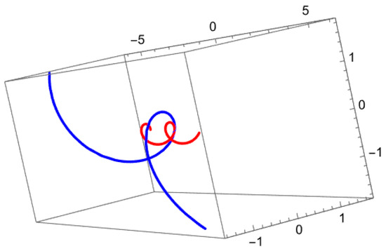
Since $T^{*}\left(f\left(s\right)\right)=\sqrt{2+2s^2}T\left(s\right),$ the vectors T and $T^{*}$ are parallel. This implies that the curves φ and ${\phi }^{*}$ are Cartan null curves with pseudo arc-length parameter, related by a Combescure transformation (See Figure 1).

Figure 1. The blue graphic is $\phi$ and the red graphic is ${\phi }^{★}$ in Example 1.

4. Solutions of the Da Rios Vortex Filament Equation Generated by Combescure-Related Cartan Null Curves

In this section, by using a given Cartan null curve and its Combescure-related Cartan null mate curve, the differentiable function $C\left(s\right)$ appearing in the parametrization of the mate curve is determined so that the ruled surface $S^{*}$ generated by the mate curve provides a solution to the Da Rios vortex filament equation. As a result, new solutions to the Da Rios vortex filament equation are obtained.

Theorem 4.

Let $\phi :I\subseteq \mathbb{R}\to {\mathbb{E}}_1^3$ and ${\phi }^{*}:I^{*}\subseteq \mathbb{R}\to {\mathbb{E}}_1^3$ be Cartan null curves related by transformation of Combescure with Frenet apparatus $\{T,N,B,\kappa ,\tau ,s\}$ and $\{T^{*},N^{*},B^{*},{\kappa }^{*},{\tau }^{*},s^{*}\},$ respectively. If the ruled surface S generated by the curve φ satisfies the Da Rios vortex filament equation, then a necessary and sufficient condition for the Combescure-related curve ${\phi }^{*}$ to also satisfy the Da Rios vortex filament equation is that the differentiable function $C\left(s\right)$ in the parametrization of ${\phi }^{*}$ given by Equation (4) is one of the following:

1. 

Let φ be a Cartan null curve with torsion function $\tau \left(s\right)=0.$ In this case:

(a) 

If

$$C\left(s\right)={\displaystyle \frac{s^3}{6}}+{\displaystyle \frac{c_2^2}{6(s+2c_1)}}+c_3+c_{4}s+c_5{s}^2$$

then the torsion function of ${\phi }^{*}$ is ${\tau }^{*}\left(s^{*}\right)=0$, where $c_2>0.$

(b) 

If

$$\begin{array}{ccc}\hfill C\left(s\right)& =& +c_3+c_{4}s+c_5{s}^2+{\displaystyle \frac{s^3}{6}}-{\displaystyle \frac{4c_1\left(s+c_2\right)}{8d}}\hfill \\ & & \\ & & -{\displaystyle \frac{\sqrt{2}\left(8d+c_1^2{(s+c_2)}^2\right)}{8d\sqrt{d}}}arctan\left({\displaystyle \frac{c_1\left(s+c_2\right)}{2\sqrt{2d}}}\right)\hfill \end{array}$$

then the torsion function of ${\phi }^{*}$ is ${\tau }^{*}\left(s^{*}\right)=d,$ where $c_1,d\in {\mathbb{R}}^{+}.$

(c) 

If

$$\begin{array}{ccc}\hfill C\left(s\right)& =& c_3+c_{4}s+c_5{s}^2+{\displaystyle \frac{3s+d{s}^3+3c_2+3ds{c}_2^2}{6d}}\hfill \\ & & \\ & & +{\displaystyle \frac{\left(8d-c_1^2{(s+c_2)}^2\right)}{4c_{1}d\sqrt{2d}}}{tanh}^{-1}\left({\displaystyle \frac{c_1\left(s+c_2\right)}{2\sqrt{2d}}}\right)\hfill \end{array}$$

then the torsion function of ${\phi }^{*}$ is ${\tau }^{*}\left(s^{*}\right)=-d,$ where $c_1,d\in {\mathbb{R}}^{+}.$

2. 

Let φ be a Cartan null curve with torsion function $\tau \left(s\right)=c$. In this case:

(a) 

If

$$C\left(s\right)={\displaystyle \frac{1}{12c^{\frac{3}{2}}}}\left(\begin{array}{c}6\sqrt{c}(s+2c_1+2c{c}_5)-6c^{{\displaystyle \frac{3}{2}}}{c}_{4}cos\left(\sqrt{2c}(s+2c_1)\right)\hfill \\ \\ +(3\sqrt{2}+8\sqrt{2}{c}_2^2+6c^{{\displaystyle \frac{3}{2}}}{c}_3)sin\left(\sqrt{2c}(s+2c_1)\right)\hfill \\ \\ -4\sqrt{2}{c}_2^{2}tan\left({\displaystyle \frac{\sqrt{c}(s+2c_1)}{\sqrt{2}}}\right)\hfill \end{array}\right)$$

then the torsion function of ${\phi }^{*}$ is ${\tau }^{*}\left(s^{*}\right)=0,$ where $c>0,$ $c_2\ne 0,$

(b) 

If

$$\begin{array}{ccc}\hfill C\left(s\right)& =& {\displaystyle \frac{s-2c_1}{2c}}+{\displaystyle \frac{2\sqrt{2}{c}_1^{2}exp(-\sqrt{-2c}(s-2c_1))}{3c^{\frac{3}{2}}(1+exp\left(\sqrt{-2c}(s-2c_1)\right))}}\hfill \\ & & \\ & & +{\displaystyle \frac{c_3}{2}}exp\left(\sqrt{-2c}(s-2c_1)\right)\hfill \\ & & \\ & & -{\displaystyle \frac{c_4}{2}}exp(-\sqrt{-2c}(s-2c_1))+c_5\hfill \end{array}$$

then the torsion function of ${\phi }^{*}$ is ${\tau }^{*}\left(s^{*}\right)=0,$ where $c_2\ne 0$, $c<0.$

(c) 

If

$$\begin{array}{ccc}\hfill C\left(s\right)& =& c_3+c_{4}cos\left(\sqrt{2c}s\right)+c_{5}sin\left(\sqrt{2c}s\right)+{\displaystyle \frac{s}{2c}}\hfill \\ & & -\int {\displaystyle \frac{8c}{(c_1+\sqrt{c_1^2-16dc}sin{(\sqrt{2k}s+c_2)}^2}}ds\hfill \\ & & +cos\left(\sqrt{2c}s\right)\int {\displaystyle \frac{8ccos\left(\sqrt{2c}s\right)}{(c_1+\sqrt{c_1^2-16dc}sin{(\sqrt{2k}s+c_2)}^2}}ds\hfill \\ & & +sin\left(\sqrt{2c}s\right)\int {\displaystyle \frac{8csin\left(\sqrt{2c}s\right)}{(c_1+\sqrt{c_1^2-16dc}sin{(\sqrt{2k}s+c_2)}^2}}ds\hfill \end{array}$$

then the torsion function of ${\phi }^{*}$ is ${\tau }^{*}\left(s^{*}\right)=d,$ where $c>0,d\in {\mathbb{R}}_0.$

(d) 

If

$$\begin{array}{ccc}\hfill C\left(s\right)& =& c_3+c_4{e}^{\sqrt{-2c}s}+c_5{e}^{-\sqrt{-2c}s}+{\displaystyle \frac{s}{2c}}\hfill \\ & & \\ & & -\int {\displaystyle \frac{8c}{(c_1+\sqrt{16dc-c_1^2}sinh{\left(\sqrt{-2c}(s+c_2)\right)}^2}}ds\hfill \\ & & \\ & & +e^{\sqrt{-2c}s}\int {\displaystyle \frac{4c{e}^{-\sqrt{-2c}s}}{(c_1+\sqrt{16dc-c_1^2}sinh{\left(\sqrt{-2c}(s+c_2)\right)}^2}}ds\hfill \\ & & \\ & & +e^{-\sqrt{-2c}s}\int {\displaystyle \frac{4c{e}^{\sqrt{-2c}s}}{(c_1+\sqrt{16dc-c_1^2}sinh{\left(\sqrt{-2c}(s+c_2)\right)}^2}}ds\hfill \end{array}$$

then the torsion function of ${\phi }^{*}$ is ${\tau }^{*}\left(s^{*}\right)=d,$ where $c<0,d\in {\mathbb{R}}_0.$

Proof. 

Let us assume that the curves $\phi$ and ${\phi }^{*}$ are Combescure-related Cartan null curves in the Minkowski 3-space, and that the ruled surface S generated from $\phi$ is a solution of the Da Rios vortex filament equation. Then, by Theorem 4, $\phi$ must be either a null Cartan cubic or a null Cartan helix. In order for the ruled surface $S^{*},$ generated by the Combescure-related curve ${\phi }^{*}$, to also be a solution of the Da Rios vortex filament equation, we need to determine the differentiable function $C\left(s\right)$ given in the parameterization of ${\phi }^{*}.$

We consider the following two cases:

Case 1: Assume that $\phi$ is a null Cartan cubic. In this case, the torsion $\tau =0.$ For the ruled surface $S^{*}$, generated by ${\phi }^{*}$, to be a solution of the Da Rios vortex filament equation, ${\phi }^{*}$ must also be either a null Cartan cubic or a null Cartan helix.

Suppose ${\phi }^{*}$ is a null Cartan cubic, then ${\tau }^{*}=0.$ Using this in Equation (15)$,$ we obtain

$$0=-{\displaystyle \frac{f^{‴}}{{\left(f^{\prime }\right)}^3}}+{\displaystyle \frac{3{\left(f^{″}\right)}^2}{2{\left(f^{\prime }\right)}^4}}$$

(28)

Solving differential Equation (28), we find that the general solution is

$$f\left(s\right)=-{\displaystyle \frac{c_2}{s+2c_1}}+c_3$$

(29)

Taking the derivative of (29) with respect to s and substituting into Equation (5) gives

$${\displaystyle \frac{c_2}{{\left(s+2c_1\right)}^2}}=\sqrt{1-{\displaystyle \frac{d^{3}C\left(s\right)}{d{s}^3}}}.$$

(30)

From (30), it is clear that $c_2>0.$ Squaring both sides yields

$${\displaystyle \frac{c_2^2}{{\left(s+2c_1\right)}^4}}=1-{\displaystyle \frac{d^{3}C\left(s\right)}{d{s}^3}}.$$

(31)

The general solution to this differential equation is

$$C\left(s\right)={\displaystyle \frac{s^3}{6}}+{\displaystyle \frac{c_2^2}{6\left(s+2c_1\right)}}+c_3+c_{4}s+c_5{s}^2$$

(32)

where $c_3,c_4$ and $c_5$ are real constants.

Now assume that ${\phi }^{*}$ is a null Cartan helix. Then, for a non-zero real constant d, we have ${\tau }^{*}=d.$ Substituting $\tau =0$ and ${\tau }^{*}=d$ into Equation (15) gives

$$d=-{\displaystyle \frac{f^{‴}}{{\left(f^{\prime }\right)}^3}}+{\displaystyle \frac{3{\left(f^{″}\right)}^2}{2{\left(f^{\prime }\right)}^4}}.$$

(33)

Solving (6), we obtain the following general solutions

For $d>0,$

$$f\left(s\right)={\displaystyle \frac{\sqrt{2}}{\sqrt{d}}}arctan\left({\displaystyle \frac{c_1(s+c_2)}{2\sqrt{2d}}}\right)+c_3.$$

(34)

For $d<0,$

$$f\left(s\right)=-{\displaystyle \frac{\sqrt{2}}{\sqrt{-d}}}arctan\left({\displaystyle \frac{c_1(s+c_2)}{2\sqrt{-2d}}}\right)+c_3.$$

(35)

Now by using $d>0$ and differentiating (34) with respect to s and substituting into Equation (15), we get

$${\displaystyle \frac{4c_1}{8d+c_1^2{\left(s+2c_1\right)}^2}}=\sqrt{1-{\displaystyle \frac{d^{3}C\left(s\right)}{d{s}^3}}}$$

(36)

Here, it is evident that $c_1>0.$ Squaring both sides of (36) leads to

$${\left({\displaystyle \frac{4c_1}{8d+c_1^2{\left(s+2c_1\right)}^2}}\right)}^2=1-{\displaystyle \frac{d^{3}C\left(s\right)}{d{s}^3}}.$$

(37)

The general solution to this equation is

$$C\left(s\right)={\displaystyle \frac{s^3}{6}}-{\displaystyle \frac{4c_1\left(s+c_2\right)}{8d}}-{\displaystyle \frac{\sqrt{2}\left(8d+c_1^2{(s+c_2)}^2\right)}{8d\sqrt{d}}}arctan\left({\displaystyle \frac{c_1\left(s+c_2\right)}{2\sqrt{2d}}}\right)+c_3+c_{4}s+c_5{s}^2$$

For $d<0,$ similar steps yield the following result

$$C\left(s\right)={\displaystyle \frac{3s+d{s}^3+3c_2+3ds{c}_2^2}{-6d}}+{\displaystyle \frac{\left(8d-c_1^2{(s+c_2)}^2\right)}{4c_{1}d\sqrt{-2d}}}{tanh}^{-1}\left({\displaystyle \frac{c_1\left(s+c_2\right)}{2\sqrt{-2d}}}\right)+c_3+c_{4}s+c_5{s}^2$$

Case 2: Now, assume that $\phi$ is a null Cartan helix, so its torsion is $\tau =c$, where c is a non-zero real constant. Then, for the ruled surface $S^{*}$, generated by ${\phi }^{*},$ to be a solution of the Da Rios vortex filament equation, the curve ${\phi }^{*}$ must again be either a null Cartan cubic or a null Cartan helix. The proof follows similarly to Case 1, and thus the second part of Theorem 4 is proven. □

Example 2.

Consider the null Cartan helix in Minkowski 3-space given by

$$\phi \left(s\right)=\left(-{\displaystyle \frac{s}{2}},{\displaystyle \frac{1}{4}}sin2s,{\displaystyle \frac{1}{4}}cos2s\right)$$

with curvatures $\kappa \left(s\right)=1,$ $\tau \left(s\right)=2$ and Frenet vectors

$$T\left(s\right)={\displaystyle \frac{1}{2}}\left(-1,cos2s,-sin2s\right)$$

$$N\left(s\right)=\left(0,-sin2s,-cos2s\right)$$

$$B\left(s\right)=\left(1,cos2s,-sin2s\right).$$

If we take $c=2,$ $c_2=1$ and $c_1=c_3=c_4=c_5=0$ in part (2a) of Theorem 4, then it follows that

$$C_1\left(s\right)={\displaystyle \frac{1}{24}}\left(6s+11sin2s-4tans\right).$$

(38)

Substituting (38) in (4), the curve ${\phi }_1^{*},$ which is Combescure-related to $\phi ,$ is obtained as follows

$${\phi }_1^{*}\left(f_1\left(s\right)\right)=\left(\begin{array}{c}-{\displaystyle \frac{1}{6}}(2+cos2s){sec}^{2}stans,\\ \\ {\displaystyle \frac{1}{6}}{sec}^{3}ssin3s,\\ \\ -{\displaystyle \frac{1}{4}}(1+2{sec}^{2}s)\end{array}\right)$$

with curvatures ${\kappa }_1^{*}\left(f_1\left(s\right)\right)=1,$ ${\tau }_1^{*}\left(f_1\left(s\right)\right)=0.$ Where $f_1\left(s\right)=tans.$

If we take $c=2,d=-1$ and $c_1=c_2=c_3=c_4=c_5=0$ in part (2c) of Theorem 4, then it follows that

$$C_2\left(s\right)={\displaystyle \frac{s}{4}}+sin\left(2s\right)ln\left(tans\right)$$

(39)

Substituting (39) in (4), the curve ${\phi }_2^{*},$ which is Combescure-related to $\phi ,$ is obtained as follows

$${\phi }_2^{*}\left(f\left(s\right)\right)=\left({\displaystyle \frac{1}{4}}(cots-tans),-{\displaystyle \frac{1}{4}}cscssecs,{\displaystyle \frac{1}{s}}ln(cots)\right)$$

with curvatures ${\kappa }_1^{*}\left(f_2\left(s\right)\right)=1,$ ${\tau }_1^{*}\left(f_2\left(s\right)\right)=-1.$ Where $f_2\left(s\right)={\displaystyle \frac{1}{\sqrt{2}}}(s\sqrt{1+s^2}-ln(-\sqrt{2}s+\sqrt{2+2s^2})).$

$$\varphi \left(s,t\right)=\left(-{\displaystyle \frac{1}{2}}+2t,{\displaystyle \frac{1}{2}}cos2s,-{\displaystyle \frac{1}{2}}sin2s\right),$$

$${\varphi }_1\left(f_1\left(s\right),t\right))=\left(\begin{array}{c}t-{\displaystyle \frac{1}{2}}{sec}^{2}s,\\ \\ 1+t-{\displaystyle \frac{1}{2}}{sec}^{2}s,\\ \\ -tans\end{array}\right),$$

$${\varphi }_2\left(f_2\left(s\right),t\right))=\left(-{\displaystyle \frac{1}{\sqrt{2}}}csc2s,{\displaystyle \frac{1}{\sqrt{2}}}cot2s,-{\displaystyle \frac{1+2t}{\sqrt{2}}}\right).$$

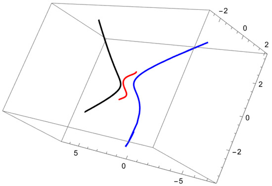
Figure 2 and Figure 3 are shown the example’s curves and surfaces.

Figure 2. The red graph represents the main curve ($\phi$), while the blue (${\phi }_1^{★}$) and black (${\phi }_2^{★}$) graphs illustrate the Combescure mate curves of the main curve in Example 2.

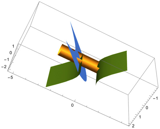
Figure 3. In Example 2, the ruled surface generated by the main curve and satisfying the Da Rios equation is shown in yellow, while the ruled surfaces generated by the Combescure mate curves of the main curve and also satisfying the Da Rios vortex filament equation are depicted in blue and green.

5. Conclusions

In this study, we have investigated Cartan null curves in Minkowski 3-space and their counterparts related via the Combescure transformation. The necessary conditions for establishing such connections were derived, and the relationships between the Frenet vectors and curvatures of these curve pairs were thoroughly analyzed. Additionally, we determined the conditions under which ruled surfaces generated by Combescure-related Cartan null curves satisfy the Da Rios equation. All results were illustrated with concrete examples, demonstrating the applicability and effectiveness of the proposed framework. These findings not only deepen the understanding of the geometric properties of Cartan null curves but also provide a systematic approach for generating new solutions to the Da Rios vortex filament equation. Future work may explore further generalizations to higher-dimensional Minkowski spaces.

References

- Miller, J. Note on Tortuous Curves. Proc. Edinburgh Math. Soc. 1905, 24, 51–55. [Google Scholar] [CrossRef]
- Bertrand, J.M. Mémoire sur la théorie des courbes á double courbure. J. Math. Pures Appl. 1850, 15, 332–350. [Google Scholar]
- Hanif, M.; Hou, Z.; Nisar, K. On special kinds of involute and evolute curves in 4-dimensional Minkowski space. Symmetry 2018, 10, 317. [Google Scholar] [CrossRef]
- Li, Y.; Kecilioglu, O.; İlarslan, K. Generalized Bertrand Curve Pairs in Euclidean Four-Dimensional Space. Axioms 2025, 14, 253. [Google Scholar] [CrossRef]
- Liu, H.; Wang, F. Mannheim partner curves in 3-space. J. Geom. 2008, 88, 120–126. [Google Scholar] [CrossRef]
- Song, X.; Li, E.; Pei, D. Legendrian dualities and evolute-involute curve pairs of spacelike fronts in null sphere. J. Geom. Phys. 2022, 178, 104543. [Google Scholar] [CrossRef]
- Zhu, M.; Yang, H.; Li, Y.; Abdel-Baky, R.A.; AL-Jedani, A.; Khalifa, M. Directional developable surfaces and their singularities in Euclidean 3-space. Filomat 2024, 38, 11333–11347. [Google Scholar] [CrossRef]
- Graustein, W.C. On two related transformations of space curves. Am. J. Math. 1917, 39, 233–240. [Google Scholar] [CrossRef]
- Camcı, Ç.; Uçum, A.; İlarslan, K. Space curves related by a transformation of Combescure. J. Dyn. Syst. Geom. Theor. 2021, 19, 271–287. [Google Scholar] [CrossRef]
- Bataray, B.; Camcı, Ç. Applications of Equivalent Curves to Ruled Surfaces. Int. Electron. J. Geom. 2025, 18, 135–142. [Google Scholar] [CrossRef]
- Kilian, M.; Müller, C.; Tervooren, J. Smooth and discrete cone-nets. Results Math. 2023, 78, 110. [Google Scholar] [CrossRef]
- Pirahmad, O.; Pottmann, H.; Skopenkov, M.B. Area preserving Combescure transformations. Results Math. 2025, 80, 27. [Google Scholar] [CrossRef]
- Pottmann, H.; Wallner, J. The focal geometry of circular and conical meshes. Adv. Comput. Math. 2008, 29, 249–268. [Google Scholar] [CrossRef][Green Version]
- Terng, C.-L. Geometric transformations and soliton equations. In Handbook of Geometric Analysis; Advanced Lectures in Mathematics (ALM), International Press: Somerville, MA, USA, 2010; Volume 2, pp. 301–358. [Google Scholar]
- Lopez, R. Differential geometry of curves and surfaces in Lorentz-Minkowski space. Int. Electron. J. Geom. 2014, 7, 44–107. [Google Scholar] [CrossRef]
- O’Neill, B. Semi-Riemannian Geometry. With Applications to Relativity; Pure and Applied Mathematics, 103; Academic Press, Inc.: New York, NY, USA, 1983. [Google Scholar]
- Keçilioğlu, O.; İlarslan, K. Combescure related pseudo null curves and their applications to Da Rios vortex filament equation. U.P.B. Sci. Bull. Ser. A 2025, 87, 99–112. [Google Scholar]
- Da Rios, L.S. On the motion of an unbounded fluid with a vortex filament of any shape. Rend. Circ. Mat. Palermo 1906, 22, 117–135. [Google Scholar] [CrossRef]
- Arms, R.J.; Hama, F.R. Localized-induction concept on a curved vortex and motion of an elliptic vortex ring. Phys. Fluids 1965, 8, 553–559. [Google Scholar] [CrossRef]
- Betchov, R. On the curvature and torsion of an isolated vortex filament. J. Fluid Mech. 1965, 22, 471–479. [Google Scholar] [CrossRef]
- Erdoğdu, M.; Özdemir, M. Geometry of Hasimoto surfaces in Minkowski 3-Space. Math. Phys. Anal. Geom. 2014, 17, 169–181. [Google Scholar] [CrossRef]
- Rogers, C.; Schief, W.K. Bäcklund and Darboux Transformations Geometry and Modern Applications in Soliton Theory; Cambridge University Press: Cambridge, UK, 2002. [Google Scholar]
- Ding, Q.; Inoguchi, J. Schrödinger flows, binormal motion for curves and the second AKNS-hierarchies. Chaos Solitons Fractals 2004, 21, 669–677. [Google Scholar] [CrossRef]
- Gürbüz, N. The motion of timelike surfaces in timelike geodesic coordinates. Int. J. Math. Anal. 2010, 4, 349–356. [Google Scholar]
- Grbović, M.; Nešović, E. On Bäcklund transformation and vortex filament equation for null Cartan curve in Minkowski 3-space. Math. Phys. Anal. Geom. 2016, 19, 23. [Google Scholar] [CrossRef]
- Couto, I.T.; Lymberopoulos, A. Introduction to Lorentz Geometry Curves and Surfaces; CRC Press, Taylor and Francis Group: Boca Raton, FL, USA, 2021. [Google Scholar]
- Duggal, K.L.; Jin, D.H. Null Curves and Hypersurfaces of Semi-Riemannian Manifolds; World Scientific: Singapore, 2007. [Google Scholar]
Disclaimer/Publisher’s Note: The statements, opinions and data contained in all publications are solely those of the individual author(s) and contributor(s) and not of MDPI and/or the editor(s). MDPI and/or the editor(s) disclaim responsibility for any injury to people or property resulting from any ideas, methods, instructions or products referred to in the content. |
© 2025 by the authors. Licensee MDPI, Basel, Switzerland. This article is an open access article distributed under the terms and conditions of the Creative Commons Attribution (CC BY) license (https://creativecommons.org/licenses/by/4.0/).