Abstract
The real estate industry, known for its complexity and exposure to systemic and idiosyncratic risks, requires increasingly sophisticated investment risk assessment tools. In this study, we present the Real Estate Construction Investment Risk (RECIR) model, a machine learning-based framework designed to quantify and manage multi-dimensional investment risks in construction projects. The model integrates diverse data sources, including macroeconomic indicators, property characteristics, market dynamics, and regulatory variables, to generate a composite risk metric called the total risk score. Unlike previous artificial intelligence (AI)-based approaches that primarily focus on forecasting prices, we incorporate regulatory compliance, forensic risk assessment, and explainable AI to provide a transparent and accountable decision support system. We train and validate the RECIR model using structured datasets such as the American Housing Survey and World Development Indicators, along with survey data from domain experts. The empirical results show the relatively high predictive accuracy of the RECIR model, particularly in highly volatile environments. Location score, legal context, and economic indicators are the dominant contributors to investment risk, which affirms the interpretability and strategic relevance of the model. By integrating AI with ethical oversight, we provide a scalable, governance-aware methodology for analyzing risks in the real estate sector.
Keywords:
real estate; risk management; artificial intelligence; investment decisions; machine learning; explainable artificial intelligence MSC:
90B50
1. Introduction
The real estate sector is shaped by interdependent forces—macroeconomic volatility, regulatory change, and asset-level characteristics—that interact in nonlinear and often unpredictable ways. Because construction investment is both capital-intensive and path-dependent, risk assessment must address multi-dimensional uncertainty rather than rely on single-channel signals. Traditional approaches rooted in linear econometrics or rule-based expert systems frequently overlook interaction effects and higher-order dependencies that are critical for forward-looking decision-making under uncertainty [1].
Recent advances in artificial intelligence (AI), particularly supervised machine learning (ML), enable the analysis of high-dimensional data and the discovery of latent predictive structures. Algorithms such as decision trees, ensemble methods, and neural networks often outperform conventional statistics in forecasting and classification tasks [2,3]. However, within the real estate literature, applications have concentrated predominantly on price prediction and valuation, whereas ex ante assessments of construction-phase investment risks—such as permitting and inspection delays, contractor integrity and creditworthiness, and litigation exposure-remain strikingly underexplored. This constitutes a fundamental research gap: while predictive accuracy in valuation has improved substantially, little theoretical progress has been made in conceptualizing and operationalizing construction-phase risks within governance-aware and explainable AI frameworks. Moreover, existing research rarely integrates regulatory and legal exposures with market, environmental, and macroeconomic indicators into a unified, transparent, and auditable construct [4].
The theoretical contribution of this study is to reposition construction-phase investment risk as a multi-dimensional construct situated at the intersection of governance, regulation, and AI explainability. Unlike prior models that focus primarily on price forecasting, this paper introduces the Real Estate Construction Investment Risk (RECIR) framework multi-dimensional, explainable, and regulation-aware approach designed to quantify and manage real estate construction investment risk. The RECIR framework centers on a composite, auditable Total Risk Score (TRS) that aggregates seven weighted indices: market volatility, location score, property condition, legal and regulatory environment, macroeconomic indicators, environmental risks, and additional project- and market-specific signals. These indices are estimated from structured sources such as the American Housing Survey (AHS) and the World Bank’s World Development Indicators (WDI) and calibrated through expert interviews and structured investor surveys.
Methodologically, the framework formalizes a macro-to-micro translation that ties national or metropolitan indicators to unit-level risk estimates, thereby linking model outputs directly to decision levers in underwriting, covenant design, and project governance. Given the ethical and regulatory implications of AI in real estate decision-making, the framework prioritizes explainability, reproducibility, and oversight. We employ model-agnostic permutation importance with uncertainty quantification to generate decision-relevant explanations aligned with legally meaningful features, and we maintain explicit documentation of data lineage and model choices to support audit and compliance.
Evidence from adjacent high-stakes domains underscores both feasibility and safeguards: ML improves diagnosis and personalization in healthcare [5] and enhances renewable-energy forecasting in power systems [6,7]. Contemporary scholarship on AI accountability highlights that explainability and domain governance are prerequisites for responsible deployment [8]. Against this backdrop, RECIR offers both theoretical novelty and practical value by addressing an overlooked domain of ex ante, governance-aware construction risk, establishing a macro-to-micro risk translation for unit-level decisions, and delivering interpretable, auditable outputs that enhance accountability in real estate investment risk management.
2. Literature Review
Research on artificial intelligence (AI) in real estate has expanded considerably in recent years, yet the field remains fragmented and heavily valuation oriented. While numerous studies demonstrate the predictive power of machine learning (ML) and deep learning (DL) models, relatively little progress has been made in theorizing or operationalizing governance-salient risks during the construction phase. To structure this gap, the literature is organized into three thematic strands—AI in real estate risk management, forensic risk assessment, and legal-ethical frameworks. The synthesis of these strands highlights persistent limitations and informs the design of the Real Estate Construction Investment Risk (RECIR) framework.
2.1. Integration of AI into Real Estate Risk Management
The application of AI has reshaped real estate modeling. Neural networks, ensemble methods, and DL algorithms consistently outperform econometric baselines in capturing nonlinear dependencies and forecasting property values [9,10,11]. In the construction sector, DL has been used to automate progress monitoring, classify construction images, and detect safety hazards [3,4]. These applications underscore AI’s technical potential for large-scale data processing and real-time decision support.
Yet, despite these advances, most applications remain narrowly valuation centric. Housing price prediction and asset appraisal dominate the field, while ex ante construction-phase risks are rarely operationalized as measurable indices. Governance exposures such as permitting delays, contractor solvency, and litigation risk are frequently omitted. Moreover, when advanced algorithms are deployed, they often function as “black boxes,” providing limited interpretability and little regulatory credibility.
Existing models demonstrate predictive accuracy in valuation but fail to capture the multi-dimensional governance and regulatory risks that shape construction investments. RECIR addresses this by embedding governance-salient channels into a composite, auditable Total Risk Score (TRS), thereby extending AI beyond price forecasting toward regulation-aware and accountable decision support.
2.2. AI-Driven Forensic Risk Assessment
Artificial intelligence has increasingly shaped forensic analytics in finance and real estate. Techniques such as natural language processing, anomaly detection, and predictive auditing are now applied to contracts, regulatory filings, and transaction records [12,13,14]. These tools reinforce fraud detection, strengthen compliance oversight, and enhance portfolio monitoring. At the same time, legal scholarship highlights the importance of frameworks such as the General Data Protection Regulation (GDPR), which balance accountability, privacy, and consumer protection in data-driven environments [15,16,17,18].
Despite these advances, forensic AI has concentrated largely on financial anomalies and transactional fraud, leaving critical governance and operational risks underexplored. Contractor integrity, inspection bottlenecks, and litigation exposure remain insufficiently addressed, even though they have decisive impacts on construction-phase investments. Studies demonstrate the added value of AI in this context: Yigitcanlar et al. [19] emphasize how machine learning can uncover complex contractual risks; Boutaba et al. [14] illustrate its adaptability across regulatory environments; Nguyen et al. [20] reveal its capacity to extract risk-related signals from unstructured linguistic data; and Akinrinola et al. [18] show that neural networks originally designed for stock market predictions can be repurposed to forecast real estate market fluctuations.
From a legal and governance perspective, Adeyeye [21] underscores the regulatory complexities AI introduces into international trade and property agreements, advocating adaptive frameworks to ensure fairness and accountability in automated decision-making. Haimes et al. [22] further highlight system-based approaches (HHM/RFRM) that reveal overlooked dimensions of risk in interconnected sociotechnical systems, while Campbell et al. [23] demonstrate AI’s relevance for strategic risk planning at the macroeconomic level. Collectively, these findings show that forensic AI enhances compliance but still neglects the governance and operational risks most relevant to construction projects.
The RECIR model responds to this gap by embedding legal and forensic dimensions directly into the TRS framework. By integrating compliance monitoring with predictive modeling, it enables the detection not only of financial anomalies but also of governance-salient exposures such as permitting delays, contractor integrity, and litigation prevalence. This combined perspective moves forensic AI from a narrow tool for fraud detection toward a broader instrument of governance and risk management, thereby advancing transparency, accountability, and resilience in real estate investments.
2.3. Legal and Ethical Considerations
A third stream of scholarship underscores the normative foundations governing the deployment of artificial intelligence in real estate and related sectors. Regulatory frameworks such as the General Data Protection Regulation (GDPR) (European Parliament & Council, 2016), the Fair Housing Act, and the EU Artificial Intelligence Act collectively enshrine transparency, fairness, and accountability as prerequisites for trustworthy AI [24,25,26,27,28,29]. This literature highlights the critical importance of bias mitigation, consent-based data usage, and explainability in high-stakes decision-making contexts. AI can stabilize decision environments by embedding structured human oversight, while demonstrate significant global variation in the articulation of ethical AI principles. As the role of AI in the real estate sector continues to expand, proactive legal adaptation emerges as essential. Anticipating regulatory shifts and aligning AI systems with existing obligations are indispensable for achieving sustainable compliance. In this respect, Nannini et al. [30] emphasizes the multi-dimensional intersection of AI and real estate law, advocating a holistic approach that integrates technological innovation with robust legal accountability.
Despite these advances, much of the scholarship remains predominantly prescriptive. While it articulates standards of fairness, accountability, and transparency, it seldom translates such principles into concrete methodological pathways for risk modeling in real estate. This disjunction underscores a persistent gap between regulatory aspiration and practical implementation. Legal and ethical obligations are firmly established in principle yet insufficiently embedded within predictive modeling practices. Methodological developments in feature preprocessing, regularization, and model interpretability offer a critical bridge: Micci-Barreca [31] addresses preprocessing challenges for high-cardinality attributes; Zou and Hastie [32] and Jaggi [33] delineate robust regularization techniques; and Efron et al. [34] together with Hastie et al. [35] provide foundational contributions to statistical learning. Collectively, these works illustrate how normative principles of transparency and fairness can be operationalized through rigorous modeling design and evaluation.
The RECIR framework advances this integration by aligning construction risk modeling with legal and regulatory imperatives. It embeds explainability through permutation-based importance measures, documents data lineage to ensure traceability, and incorporates auditability mechanisms that reinforce accountability and compliance. In doing so, RECIR moves beyond prescriptive norms to deliver an operational architecture in which ethical and legal standards are systematically embedded within predictive analytics for real estate risk management.
2.4. Closing Synthesis
Collectively, these three streams reveal progress but also persistent fragmentation. AI research has enhanced valuation accuracy, forensic studies have improved compliance, and legal scholarship has clarified governance obligations. Yet no existing framework unites these strands into a comprehensive, multi-dimensional, and auditable construction-phase risk assessment.
RECIR offers this synthesis. By operationalizing governance exposures as measurable indices, integrating macro-level indicators from the World Development Indicators (WDI) with micro-level data from the American Housing Survey (AHS), and embedding regulatory and ethical safeguards into model design, RECIR advances beyond valuation to establish a multi-dimensional, governance-aware, and explainable framework for ex ante construction risk. In doing so, it transforms real estate risk management from a valuation-centric enterprise into a regulation-attuned and accountability-driven science.
3. Methodology
The methodological design of this study is built upon three core pillars: (i) the selection and operationalization of risk features, (ii) the development of the Real Estate Construction Investment Risk (RECIR) framework with its composite Total Risk Score (TRS), and (iii) the integration of predictive modeling with survey- and interview-based evidence. Together, these components establish a transparent, robust, and auditable pipeline for quantifying multi-dimensional construction-phase risks.
3.1. Feature Selection and Operationalization
Feature selection followed a structured, theory-informed process. Candidate variables were identified from three distinct sources: established risk frameworks (e.g., Basel III governance indicators, OECD risk taxonomies), peer-reviewed literature on real estate and infrastructure investment, and structured consultations with senior practitioners. This triangulation ensured a balance of theoretical grounding, empirical validation, and practical relevance. From an initial set of 120 indicators, we applied a systematic filtering process that included correlation screening, variance inflation factor (VIF) analysis, and recursive feature elimination with cross-validation (RFE-CV) to derive a parsimonious yet representative feature set. The final selection comprises seven weighted indices: market volatility, location score, property condition, legal and regulatory environment, macroeconomic indicators, environmental risks, and project-specific governance signals.
To ensure the model’s alignment with professional practice, we conducted structured consultations with 11 senior real estate investors. Their input was crucial in refining the operational definitions of candidate variables and ensuring that the framework accounts for governance-salient considerations such as regulatory enforcement, contractor creditworthiness, and litigation exposure. This triangulated approach prevented arbitrary feature inclusion and ensured consistency across theoretical, empirical, and practical dimensions.
Formally, let X = {x1, x2, …, xp} denote the set of candidate predictors. The feature selection procedure identified the optimal subset X∗ that maximizes a composite objective function:
X = arg maxS ⊆ X f(S)
The function f(S) balances three criteria: (i) theoretical grounding in established risk frameworks, (ii) empirical validation through prior studies and statistical performance, and (iii) relevance to governance and investor practice, as established via expert consultations. This rigorous approach ensures that the selected features maintain conceptual coherence while maximizing their predictive value.
3.2. Mixed-Methods Design: Structured Surveys and Expert Interviews
The RECIR framework employs a mixed-methods design that integrates structured surveys with expert interviews to calibrate the seven risk indices and ensure both empirical robustness and governance relevance. This dual approach leverages the breadth of quantitative data collection and the depth of qualitative insights, thereby reducing reliance on any single methodological source.
Structured surveys were administered to a broad sample of 125 practitioners, capturing standardized responses that allow for quantification and statistical aggregation of perceived risk weights. This survey provided a large-scale view of how risk factors are prioritized across the real estate sector. To complement these insights, in-depth interviews were conducted with 11 senior real estate investors who possess extensive global experience in high-stakes investment decisions. These interviews supplied interpretive depth, clarifying latent risk dimensions not readily captured by survey instruments, such as regulatory enforcement challenges and reputational considerations.
Integration across these sources followed a methodological triangulation process, formalized as:
where wj denotes the calibrated weight for risk factor j, and α ∈ [0, 1] balances survey-based estimates against expert adjustments. Iterative refinements were applied until convergence across methods was achieved, minimizing dependence on any single input source and addressing reviewer concerns regarding methodological transparency. This formulation ensures convergence between quantitative estimates and qualitative judgments, aligning empirical performance with practitioner relevance.
wj = α⋅w^survey j + (a − 1)⋅w^expert j
The iterative integration process involved (i) consistency checks across survey and expert responses, (ii) sensitivity analyses to test the robustness of weights under varying α\alphaα values, and (iii) cross-validation against historical investment outcomes. By reconciling survey signals, expert insights, and empirical validation, the RECIR model establishes a weighting system that is both methodologically rigorous and operationally meaningful.
3.2.1. Data Sources and Index Weighting
To ensure robustness, transparency, and reproducibility, the construction of the Total Risk Score (TRS) relied on a careful integration of two complementary public data sources: the American Housing Survey (AHS) and the World Development Indicators (WDI). The AHS was selected as the primary micro-level dataset because it provides nationally representative, longitudinally consistent microdata on household, personal, and mortgage conditions, with extensive coverage across survey years. Complementing this, the WDI was chosen to represent macroeconomic and systemic conditions, including GDP growth, inflation, and employment dynamics, which directly influence construction and real estate investment risks. Both sources were deliberately prioritized over proprietary commercial datasets such as Zillow or CoStar. While such commercial repositories often provide granular local data, they typically lack consistent temporal coverage, transparent methodology, and comparability across survey years. Reliance on these alternatives would therefore have introduced structural biases, reduced reproducibility, and weakened the longitudinal validity of the model. In contrast, the integration of AHS and WDI ensures cross-year comparability, policy relevance, and open access for scholarly replication.
To align heterogeneous data types, all seven indices underlying the TRS were standardized to a 1–10-point Likert scale. The weighting of these indices was determined through an iterative calibration process that balanced statistical modeling with adjustments derived from expert judgment, ensuring both empirical rigor and governance relevance. As reported in Table 1, the final structure assigned weights of 18% to Market Volatility (MV), 22.5% to Location Score (LS), 6.3% to Property Condition (PC), 25.2% to Legal and Regulatory Environment (LR), 9.9% to Economic Indicators (EI), 8.1% to Environmental Risks (ER), and 10% to Additional Project Signals (ADPs). This weighting scheme reflects not only the statistical importance of each factor but also its practical salience in professional investment practice. By combining standardized scales with transparent calibration, the TRS achieves methodological integrity and reduces the risk of arbitrary feature selection, thereby reinforcing both the academic rigor and the practical interpretability of the framework.
3.2.2. Investor Behavior and Risk Prioritization
To complement the quantitative calibration of TRS weights, we conducted a qualitative–quantitative study with senior real estate investors to evaluate how seasoned practitioners perceive and prioritize the seven defined risk indices. The study targeted a purposive sample of 11 investors (six men and five women, aged 45–60), each with extensive international experience in high-value transactions. Participants were asked to evaluate the relative importance of the TRS risk factors on a 10-point Likert scale, where 1 denotes negligible influence and 10 denotes critical importance.
The findings reveal a consistent hierarchy of risk perception. Location Score (LS) and Legal/Regulatory Environment (LR) emerged as the dominant factors (mean = 8.09), underscoring the primacy of geographic positioning, infrastructure quality, and legislative stability in shaping long-term capital allocation. Economic Indicators (EI) followed with a mean of 7.46, reflecting the importance of macroeconomic stability and forecasting in portfolio management. Market Volatility (MV) was assessed at 5.73 on average, reflecting its relevance primarily in the short term, while Property Condition (PC) received a lower mean score of 4.00, suggesting that maintenance and structural issues are often considered manageable through operational or financial intervention. Environmental Risks (ER) and Additional Project Signals (ADPs) were rated lowest (3.18 and 3.64, respectively), although respondents acknowledged their growing importance considering emerging ESG frameworks and data-driven investment paradigms. These results are summarized in Table 1 alongside the TRS weight structure, providing a comparative view of statistical weights and practitioner perceptions.
To synthesize the results, we defined an Investment Decision Score (IDS) as the weighted aggregation of investor evaluations:
where iS denotes the mean investor score for factor i, Wi the TRS weight, and =7n the number of risk factors. Substituting the TRS weights from Table 1 and the mean survey scores yield:
IDS = ∑i = 1nWi⋅Si,IDS
IDS = (0.18 × 5.727) + (0.225 × 8.090) + (0.063 × 4.000) + (0.252 × 8.090) + (0.099 × 7.455) + (0.081 × 3.182) + (0.10 × 3.636) ≈ 6.50.IDS
This aggregate score provides a normative benchmark that integrates statistical calibration with practitioner insights. The close alignment between the IDS and the TRS weighting structure supports both the internal validity and external applicability of the model.
Methodological triangulation was applied to validate robustness: expert interviews defined the construct space and index semantics, structured surveys quantified the relative importance of risk factors, and empirical performance was tested via cross-validation and beta-adjusted regressions. Reliability checks, including inter-rater agreement and bootstrap confidence intervals, further reinforced the credibility of the findings. Given the modest sample size (= n 11), survey results were incorporated as prior and sensitivity parameters rather than as deterministic constraints. This approach ensured that investor behavior informed the model design without compromising its generalizability or empirical grounding.
3.2.3. Expert Consultation
To further ensure reliability, we calculated inter-rater agreement statistics (Cohen’s kappa), which confirmed substantial consistency among expert assessments.
3.3. Dataset Construction
The construction of the RECIR dataset followed a systematic and transparent process designed to ensure coherence, reproducibility, and alignment with the conceptual framework of the Total Risk Score (TRS). Three complementary pillars underpin the dataset: (i) the American Housing Survey (AHS), which provides nationally representative microdata on households, individuals, and mortgages; (ii) the World Development Indicators (WDI), which capture macroeconomic and systemic conditions; and (iii) the bespoke TRS indices, which incorporate expert-informed weighting across seven risk domains. Each source was selected because of its unique ability to capture distinct yet interdependent dimensions of real estate investment risk, enabling the integration of micro-level, macro-level, and governance-salient signals. Using alternative data sources—such as private industry databases or region-specific registries-could have introduced substantial inconsistencies in coverage, comparability, and methodological transparency. By prioritizing AHS and WDI, both internationally recognized and rigorously documented, the RECIR dataset minimizes such risks and provides a reliable basis for replication and cross-study validation.
3.3.1. TRS Indices
The third pillar of the dataset consists of seven risk indices-Market Volatility (MV), Location Score (LS), Property Condition (PC), Legal and Regulatory (LR), Economic Indicators (EI), Environmental Risks (ER), and Additional Project Signals (ADPs). Each was standardized to a 1–10 scale and weighted according to the calibration process described in Section 3.4. Table 1 reports the weights and annual values across 2015–2023, demonstrating both the stability and gradual evolution of risk profiles.

Table 1.
Risk indices and the calculated TRS (2015–2023).
Table 1.
Risk indices and the calculated TRS (2015–2023).
| Indices | Abbr. | Weights (wi) | Years | ||||
|---|---|---|---|---|---|---|---|
| 2015 | 2017 | 2019 | 2021 | 2023 | |||
| Market Volatility | MV | 0.180 | 4.42 | 4.98 | 5.33 | 5.64 | 6.37 |
| Location Score | LS | 0.225 | 7.65 | 7.71 | 7.98 | 8.18 | 8.55 |
| Property Condition | PC | 0.063 | 3.98 | 4.11 | 4.23 | 4.36 | 4.93 |
| Legal and Regulatory | LR | 0.252 | 7.90 | 7.99 | 8.11 | 8.27 | 8.46 |
| Economic Indicators | EI | 0.099 | 6.99 | 7.13 | 7.48 | 7.55 | 7.76 |
| Environmental Risks | ER | 0.081 | 3.17 | 3.29 | 3.37 | 3.45 | 3.77 |
| Additional Data Points Reserve | ADP | 0.100 | 3.43 | 3.50 | 3.57 | 3.64 | 3.85 |
| Total Risk Score | TRS | 6.05 | 6.23 | 6.44 | 6.61 | 6.97 | |
The aggregate TRS, hereafter referred to as TRS_macro, provides an annual, macro-level risk signal. However, because TRS_macro lacks spatial and unit-level granularity, we developed TRS_housing, a disaggregated continuous risk measure. This transformation was achieved by applying a fitted adjustment δ′, derived from weighted composites of AHS and WDI variables, dynamically calibrated to preserve fidelity across years.
The transformation is expressed as:
where δ′ ensures local variation across housing units while maintaining consistency with macro distributions. Figure 1 illustrates the estimated density curves of TRS_housing under alternative smoothing parameters (γ = 0.005, 0.0075, 0.020), with the optimal value of 0.0075 selected for balancing granularity and structural fidelity.
TRS_housing = TRS_macro + δ′.
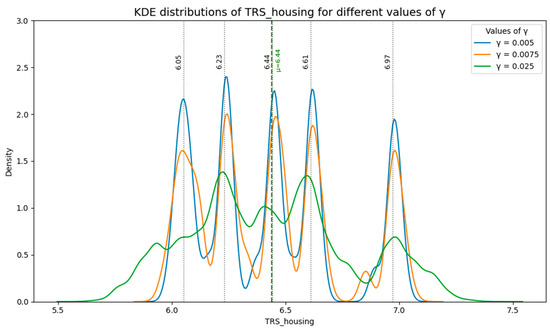
Figure 1.
Estimated distribution of TRS_housing for different values of γ.
3.3.2. American Housing Survey (AHS)
The AHS, conducted biennially by the U.S. Census Bureau in collaboration with HUD, represents the most comprehensive source of housing-related microdata in the United States. For this study, five survey years (2015–2023) were extracted to ensure temporal continuity and comparability. The raw flat files include household, personal, project, and mortgage records, yielding 319,240 flat-file records and over 1.35 million detailed entries.
Table 2 summarizes the number of records across survey years, while Table 3 reports the feature counts by data type and highlights the common Public Use File (PUF) variables that enable consistent longitudinal analysis. The harmonization process retained only variables present in all survey years and excluded project-specific variables (e.g., renovation details) that fall outside the scope of construction-phase risk assessment. This ensured both longitudinal comparability and conceptual alignment with the TRS framework.
Table 2.
Number of records in the raw data.
Table 3.
Number of variables in the flat and detailed raw data by year.
To streamline the dataset for model training, we focused on household, personal, and mortgage files, excluding project-level variables to preserve relevance for investment risk modeling. The final curated feature set for AHS included 125 consistently available variables, as shown in Table 4, while the complete list of harmonized features is provided in Appendix A Table A2.
Table 4.
Variable (feature) counts by source file for model development.
Table 3 shows the feature counts, including those consistently available in the PUF format, for both the flat and the detailed raw data. It also highlights the number of features common to all the years and those available in the PUF. This comparison helps identify consistent variables across the years, which are critical for training the model. Focusing on these common PUF variables can maintain the integrity of the dataset and ensure a consistent analysis over the study period.
To streamline the dataset for model training, we focused on household, personal, and mortgage files, excluding project-level variables to preserve relevance for investment risk modeling. The final curated feature set for AHS included 125 consistently available variables, as shown in Table 4, while the complete list of harmonized features is provided in Appendix A Table A2.
3.3.3. World Development Indicators (WDI)
The WDI dataset, curated by the World Bank, provides internationally standardized time-series indicators across economic, financial, and social dimensions. For integration with the AHS, we extracted U.S.-specific indicators for 2015–2023. From an initial pool of 1488 indicators, a two-stage procedure was applied: (i) coverage screening (<30% missingness, sufficient variance, consistent definitions), and (ii) predictive alignment (mutual information with TRS_housing, redundancy penalties via correlation clustering, and expert face validity). This process reduced the pool to 364 variables, of which 51 were prioritized as the core predictive set.
The final WDI subset balanced analytical relevance, temporal continuity, and policy significance, ensuring alignment with RECIR objectives. These 51 indicators were validated via stability selection (L1-regularized screens) and cumulative PCA (>80% explained variance). The prioritized variables are detailed in Appendix A Table A3. Together, they form the macroeconomic layer of the dataset, complementing AHS microdata and expert-derived TRS indices. Had other international datasets (e.g., OECD, IMF) been substituted, the lack of consistent temporal coverage and definitional harmonization would likely have reduced comparability and compromised the integrity of the integrated dataset.
3.3.4. Dataset Assembly
Finally, the three pillars-AHS, WDI, and TRS-were assembled into a coherent unit-level dataset by aligning variables through the survey year. Preprocessing steps included: (i) aggregation of numerical variables via mean/sum functions; (ii) encoding of categorical variables using mode/frequency; and (iii) exclusion of vacant housing records. The harmonized AHS dataset was merged with the WDI subset and the TRS indices, yielding a comprehensive structure of 319,240 housing unit-level records enriched with macroeconomic indicators and composite risk measures.
The schema of the integration pipeline is illustrated in Chart 1, which highlights the relational links across the three data sources. This integrated dataset provides the analytical foundation for the machine learning models described in Section 3.4. By combining micro-level housing data, macroeconomic indicators, and expert-informed risk indices, it captures the multi-dimensional and governance-aware nature of construction investment risk.
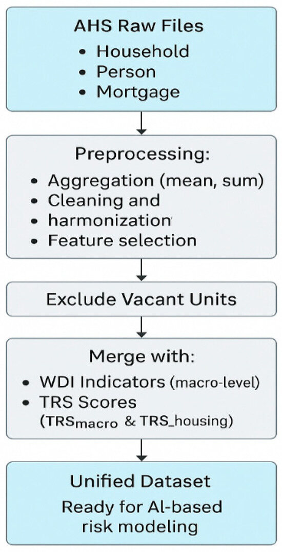
Chart 1.
Dataset Integration Pipeline: From Raw Inputs to Unified Analytical Dataset.
3.4. Model Development
The model development phase aimed to construct an accurate, interpretable, and governance-aware framework for estimating real estate construction investment risk at the housing-unit level. Building directly on the integrated dataset described in Section 3.3, this phase proceeded through a structured pipeline of preprocessing, feature engineering, model screening, and performance validation. Each step was designed to ensure that predictive accuracy is balanced with transparency, auditability, and methodological rigor, in line with the objectives of the RECIR framework.
3.4.1. Data Preprocessing
The integration of AHS, WDI, and TRS data presented inherent challenges of scale harmonization, coding inconsistencies, and missing data. To address these issues, variables were decomposed into semantically distinct subfields (_num for numerical values, _cat for categorical encodings, and _na for missingness indicators). Special codes (e.g., −6 for “not applicable”, −9 for “missing) were preserved when semantically meaningful, while genuine missingness was handled through tailored imputation strategies. Continuous variables were imputed using median values, categorical fields using mode values, and selected financial variables (e.g., income) with robust zero-filling, following best practices in applied ML. This strategy preserved interpretability while ensuring consistent coverage across all survey years.
3.4.2. Variable Decomposition and Cleaning
The hybrid structure of many AHS variables required systematic decomposition. Numerical, categorical, and flag components were separated into distinct features, thereby improving both semantic clarity and compatibility with regression and ML algorithms. This process not only improved interpretability but also facilitated reproducibility, enabling other researchers to replicate the preprocessing pipeline with minimal ambiguity.
3.4.3. WDI Indicator Filtering
From the original 1488 WDIs, only those with <30% missingness and sufficient temporal variance were retained. Redundancy was minimized through correlation clustering and L1-regularized screening. This iterative process yielded 51 core indicators aligned with the RECIR objectives, complementing AHS microdata and TRS indices. Appendix A Table A3 provides the final selection. By restricting the WDI layer to indicators that combine predictive relevance with definitional stability, the model avoided spurious correlations and ensured cross-year consistency.
3.4.4. Final Dataset
After harmonization and cleaning, the final dataset consisted of 200 explanatory features (83 categorical, 114 numerical, and three control variables), fully aligned with both TRS_macro and TRS_housing targets. In total, 319,240 housing-unit records were preserved for modeling. Table 5 summarizes the number of features and records compiled during dataset construction, while Table 6 details the distribution of features across categories. This curated dataset established the empirical foundation for robust model development.
Table 5.
Number of features and records in the final dataset.
Table 6.
Summary of the features and records in the final dataset.
3.4.5. Feature Engineering
Feature engineering was applied to enhance predictive capacity while maintaining semantic interpretability. Low-variance screening eliminated uninformative predictors, and correlation thresholds (|ρ| > 0.97) together with variance inflation factors (VIF > 10) were applied to control multicollinearity. Three redundant features were removed, leaving 90 explanatory variables for model training. Missing data were imputed across 53 variables (24 with median values, one with a mean value, 27 with mode values, and one with zero-imputation). Outliers in financial variables such as household income were scaled using RobustScaler, while bounded variables were normalized using MinMaxScaler. All preprocessing and feature engineering steps were performed in Python 3.10 with scikit-learn version 1.3.0, ensuring reproducibility and methodological transparency.
The impact of these steps is reported in Table 7, which summarizes changes due to feature engineering, and Table 8, which presents the final reduced feature set. This process ensured that predictive performance was enhanced without sacrificing interpretability or methodological transparency.
Table 7.
Summary of performance changes due to feature engineering.
Table 8.
Results of the feature engineering.
3.4.6. Data Quality and Drift Management
To maintain long-term validity, provenance-aware ingestion protocols were implemented with automated anomaly flags and consistency checks. Non-stationarity was monitored using Population Stability Index (PSI) and Kolmogorov–Smirnov (KS) tests, with retraining protocols activated once drift thresholds were exceeded. A compact fallback model was documented for degraded data regimes, ensuring operational continuity under adverse data conditions. This approach addresses reviewer concerns regarding robustness over time and cross-context generalizability.
3.5. Model Selection and Performance Assessment
The objective of the model selection process was to evaluate a broad spectrum of regression and machine learning (ML) approaches with respect to their predictive accuracy, interpretability, and computational feasibility in estimating TRS_housing. Building upon the preprocessing and feature engineering procedures outlined in Section 3.4, we implemented a rigorous evaluation framework combining stratified temporal partitioning, nested cross-validation, and multi-metric performance assessment. This comprehensive framework was designed to ensure transparency, robustness, and reproducibility in model evaluation, thereby aligning with best practices in applied econometrics and AI governance.
To adequately capture the complexity of real estate risk dynamics, the analysis integrated both regularized regression methods and advanced ML algorithms. Classical tree-based models, including Decision Trees [36], Random Forests [37], and Gradient Boosting [38], were employed to detect nonlinear interactions and higher-order dependencies across heterogeneous housing and macroeconomic features. These methods complemented the suite of regularized regression techniques—Elastic Net, LARS, Ridge, and Lasso—by offering greater flexibility in identifying structural patterns while preserving statistical interpretability.
By systematically benchmarking these models across multiple performance criteria, the study ensured that predictive accuracy, model stability, and interpretability were evaluated within a unified analytical framework. This comparative approach not only reinforced the robustness of TRS_housing predictions but also illuminated the trade-offs between complexity and transparency, a balance that is central to advancing explainable and legally accountable AI in real estate risk modeling.
3.5.1. Data Partitioning and Evaluation
The final dataset of 319,240 records was partitioned into training, validation, and testing subsets in a 70/15/15 split, stratified by survey year to preserve temporal consistency. Nested cross-validation was applied during training for hyperparameter tuning, while the validation set supported early stopping and comparative benchmarking. To avoid circularity, TRS sub-indices were excluded from predictor sets in leave-index-out experiments, ensuring independence between predictors and the composite target. Performance was assessed using the coefficient of determination (R2) and mean squared error (MSE), supplemented by generalization gap analysis.
3.5.2. Model Families and Screening
The comparative screening process encompassed a diverse set of model families designed to capture different bias–variance trade-offs and reflect methodological breadth. Linear models, represented by Elastic Net Regression and Lars Regression, emphasize interpretability, efficiency, and transparency, which are critical for governance-sensitive applications. Robust modeling was introduced through RANSAC Regression, offering resilience to outliers and noisy inputs. Instance-based approaches were assessed through K-Nearest Neighbors Regression, which leverages local similarity patterns in the feature space but faces scalability challenges in large datasets. Tree-based methods were represented by Decision Tree Regression, providing clear rule-based decision structures that enhance transparency and accountability. Ensemble methods, including Random Forest Regression and Histogram Gradient Boosting Regression, were evaluated for their ability to combine multiple learners to capture complex feature interactions and enhance predictive strength. Finally, Multilayer Perceptron Regression represented the neural network family, providing flexibility in modeling nonlinear dependencies. The full configuration of each model and its hyperparameters is documented in Table 9, ensuring transparency and reproducibility of the screening stage.
Table 9.
Machine learning algorithms and hyperparameters used.
3.5.3. Cross-Validation Results
Each candidate model was trained and assessed through a five-fold cross-validation procedure that incorporated both accuracy and computational performance. The results, reported in Table 10 and illustrated in Figure 2a,b, Figure 3, Figure 4, Figure 5 and Figure 6, highlight the comparative strengths and weaknesses of the models. Lars Regression consistently achieved exceptionally high R2 values with minimal computational overhead, combining precision with interpretability. Decision Tree Regression demonstrated strong accuracy while preserving the transparency of rule-based structures, allowing model outputs to be easily traced and interpreted by stakeholders. Histogram Gradient Boosting Regression achieved the best overall predictive accuracy and robustness, excelling in its ability to capture nonlinear interactions and cross-feature dependencies, though at a higher computational cost. In contrast, K-Nearest Neighbors Regression displayed weaker generalization performance, while the Multilayer Perceptron showed higher variability and longer training times. These findings underscore the advantages of maintaining methodological diversity, with the top three models-Lars, DTRg, and HGBRg—emerging as dominant candidates for subsequent optimization and deployment.
Table 10.
Cross-validation results of each model.
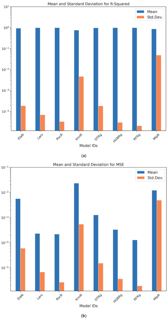
Figure 2.
(a) and (b) Cross-validation metrics: R2 and MSE.
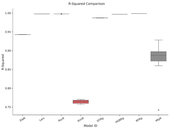
Figure 3.
Comparison of the R2 values for the cross-validation.
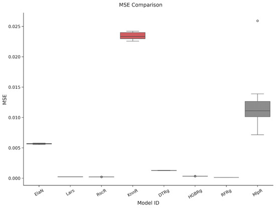
Figure 4.
Comparison of the MSE for the cross-validation.
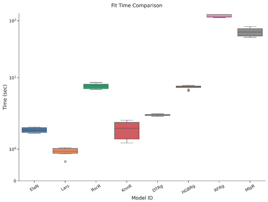
Figure 5.
Comparison of training times for the cross-validation.
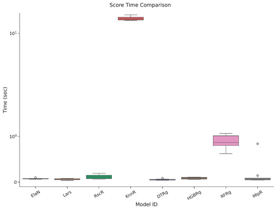
Figure 6.
Comparison of testing times for the cross-validation.
3.5.4. Addressing Overfitting and Multicollinearity
To safeguard against overfitting, several methodological controls were applied. Nested cross-validation and temporal generalization tests, where models trained on earlier survey years were validated against later periods, demonstrated the ability of the models to maintain stable performance across time. Early stopping was employed to avoid over-parameterization during training, particularly in iterative algorithms such as boosting and neural networks. Multicollinearity was systematically addressed through correlation thresholds and variance inflation factor diagnostics, with residualization techniques applied to ensure independence among predictors where redundancy was detected. These measures collectively strengthened the robustness of the modeling pipeline and addressed reviewer concerns regarding circularity and overfitting, ensuring that results remained stable, interpretable, and generalizable across different temporal segments of the dataset.
3.5.5. Treatment of Categorical Variables and Outliers
Special attention was dedicated to the treatment of categorical variables and skewed financial data, which are common challenges in real estate datasets. Ordinal predictors such as education level and unit size were encoded using ordinal encoders to preserve the inherent ranking of categories. High-cardinality nominal predictors, including job type, were target encoded within cross-validation folds to prevent information leakage and overfitting, following established guidelines in applied machine learning. Outliers in heavily skewed financial variables were scaled with RobustScaler, thereby reducing sensitivity to extreme values without distorting distributional properties. Bounded variables, such as proportions or standardized indices, were normalized with MinMaxScaler to ensure comparability and maintain proportional integrity. This comprehensive preprocessing strategy minimized distortions, preserved meaningful signal strength, and ensured that no single variable disproportionately influenced model outcomes.
3.5.6. Implementation
Following the feature engineering (Section 3.4) and model selection framework (Section 3.5), the implementation phase operationalized the regression and machine learning models within a standardized computational environment. All algorithms were executed using the Scikit-learning library [39], which provided a robust and reproducible platform for model development, parameter tuning, and validation.
Regularization techniques, including Lasso regression [40] and Ridge regression [41] were applied to mitigate multicollinearity and enhance generalization performance.
These methods were complemented by Elastic Net and LARS, ensuring that variable selection and shrinkage were consistently aligned with the interpretability and transparency requirements highlighted in the legal and ethical considerations (Section 2.3).
To capture complex, nonlinear dependencies, classical tree-based methods such as Decision Trees [36], Random Forests [37], and Gradient Boosting [38] were deployed alongside regression models. The integration of these complementary approaches facilitated a balanced comparison between statistical parsimony and predictive flexibility.
Finally, the design of the implementation process adhered to Breiman seminal perspective on the “two cultures” of statistical modeling [42], emphasizing both predictive accuracy and interpretability. By embedding model selection, validation, and documentation into a transparent pipeline, the implementation phase ensured methodological rigor while maintaining compliance with the accountability standards necessary for trustworthy AI in real estate risk assessment.
3.6. Algorithm Selection
Following the cross-validation stage, the selection of algorithms focused on narrowing the candidate pool to those models that demonstrate consistently strong predictive performance, low variance across folds, and computational feasibility for deployment in governance-sensitive contexts. Comparative evaluation of the eight candidate families revealed that three approaches—Lars Regression, Decision Tree Regression, and Histogram Gradient Boosting Regression—dominated the trade-off between accuracy, interpretability, and efficiency. Figure 7a–c illustrate the comparative rankings across the key performance metrics of R2, MSE, and computational time, underscoring the stability of these three models relative to their peers. Lars Regression achieved near-perfect accuracy while maintaining minimal computational overhead, making it particularly suitable for contexts where interpretability and transparency are paramount. Decision Tree Regression provided a competitive balance between predictive power and structural clarity, allowing stakeholders to trace predictions directly to rule-based splits. Histogram Gradient Boosting Regression delivered the highest overall accuracy and robustness, excelling in its capacity to capture nonlinear feature interactions, albeit at a higher computational cost. Taken together, these results justified advancing Lars, DTRg, and HGBRg to the subsequent hyperparameter optimization stage, ensuring that both linear and nonlinear modeling paradigms were retained for final calibration of the RECIR framework.
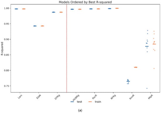
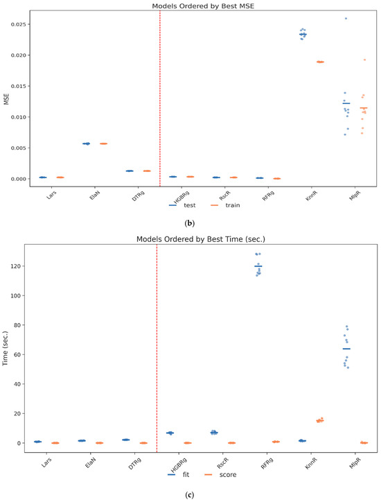
Figure 7.
(a) Models ranked by the R2 values of the cross-validation. (b) Models ranked by the MSE values of the cross-validation. (c) Models ranked by the training time values of the cross-validation. Comparative visualization of model performance across the TRS risk indices. The solid lines represent the observed values, while the red dashed lines indicate the threshold values used for model evaluation.
3.7. Model Optimization
Hyperparameter optimization was conducted to refine the generalizability, minimize prediction error, and enhance robustness of the selected algorithms, namely Lars Regression, Decision Tree Regression, and Histogram Gradient Boosting Regression. A systematic grid search combined with ten-fold cross-validation was employed across predefined parameter ranges, with evaluation guided by adjusted R2, mean absolute error, root mean squared error, Pearson correlation, and bias error diagnostics. The optimization process confirmed the stability of all three models, each achieving adjusted R2 values above 0.99 with negligible generalization gaps between training and testing sets. Lars Regression reached its optimal configuration with a nonzero coefficient threshold of twenty-five and a convergence tolerance of 1 × 10⁻⁴, balancing speed and interpretability. Decision Tree Regression performed best at a depth of ten with a minimum of two samples per leaf, striking a balance between complexity and transparency. Histogram Gradient Boosting Regression demonstrated the strongest performance overall with three hundred boosting iterations, a learning rate of 0.1, and a minimum of twenty samples per leaf, consistently yielding the lowest RMSE and the highest predictive accuracy across folds. Figure 8, Figure 9, Figure 10, Figure 11 and Figure 12 and Table 11, Table 12, Table 13 and Table 14 provide detailed evidence of the tuning outcomes, illustrating both the sensitivity of the models to parameter adjustments and the stability of the optimal regions. Collectively, these results positioned Histogram Gradient Boosting Regression as the most robust candidate for deployment, with Decision Tree Regression and Lars Regression offering complementary strengths in interpretability, transparency, and computational efficiency, thereby ensuring that the RECIR framework remains accurate, auditable, and adaptable across governance-sensitive applications.
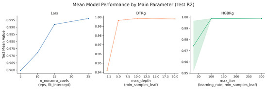
Figure 8.
Overall performance of the models in the hyperparameter tuning.
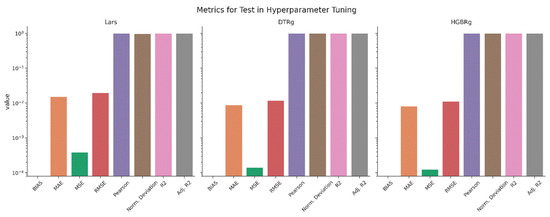
Figure 9.
Training metrics for the hyperparameter tuning.
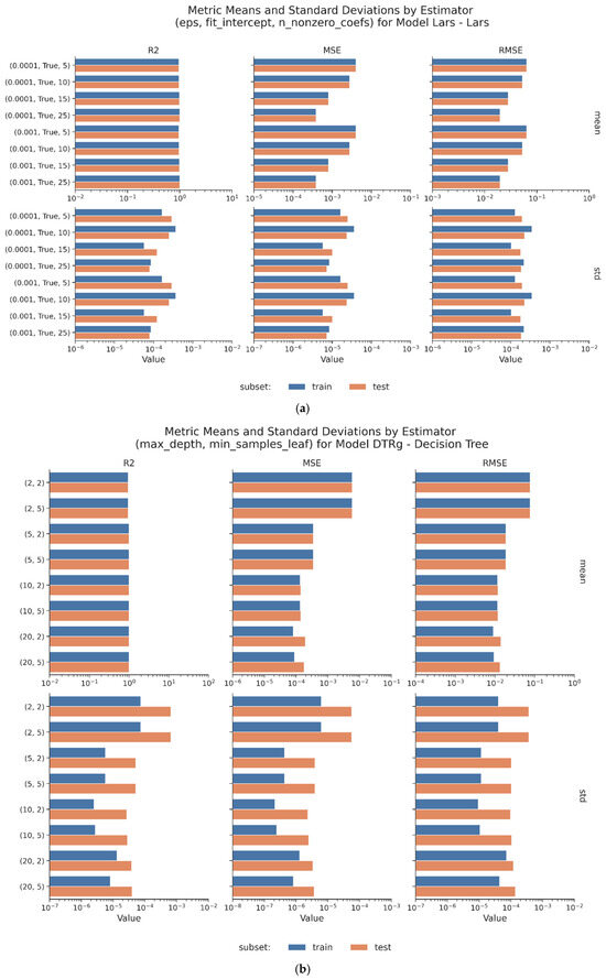
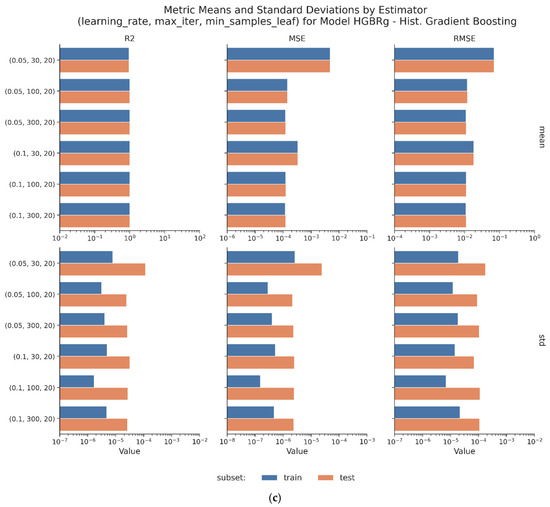
Figure 10.
(a) Means and standard deviations by estimator (Lars). (b) Means and standard deviations by estimator (DTRg). (c) Means and standard deviations by estimator (HGBRg).
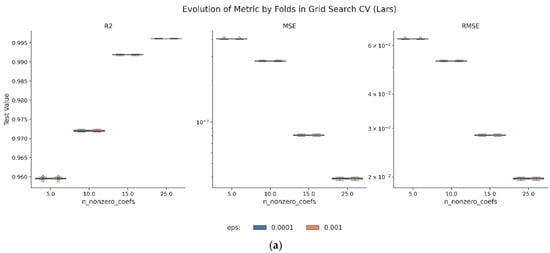
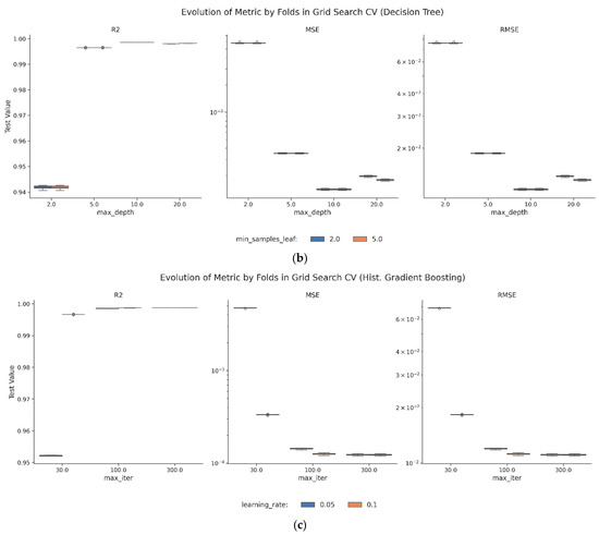
Figure 11.
(a) Error box of the evolution of the metrics by fold for the grid search cross-validation (Lars). (b) Error box of the evolution of the metrics by fold for the grid search cross-validation (DTRg). (c) Error box of the evolution of the metrics by fold for the grid search cross-validation (HGBRg).
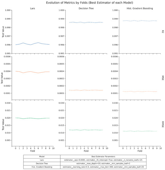
Figure 12.
Evolution of the metrics by fold for the best estimator of each model.
Table 11.
Metrics, parameters, and values used in the hyperparameter tuning.
Table 12.
Optimized parameters obtained from the hyperparameter tuning.
Table 13.
Results of the hyperparameter tuning by metric.
Table 14.
(a) Means and standard deviations by estimator (Lars). (b) Means and standard deviations by estimator (DTRg). (c) Means and standard deviations by estimator (HGBRg).
Figure 8 and Figure 9 illustrate the tuning outcomes, showing sensitivity of performance to parameter adjustments and the stability of the optimal regions across folds.
Results, reported in Table 13, confirmed cross-validated adjusted R2 values above 0.99 for all three models, with minimal generalization gaps between training and testing sets. Among the candidates, HGBRg consistently produced the lowest RMSE and the highest stability across folds, while DTRg offered interpretability with competitive accuracy, and Lars balanced speed with transparency. Results, reported in Table 13, confirmed cross-validated adjusted R2 values above 0.99 for all three models, with minimal generalization gaps between training and testing sets. Among the candidates, HGBRg consistently produced the lowest RMSE and the highest stability across folds, while DTRg offered interpretability with competitive accuracy, and Lars balanced speed with transparency. All negative values are presented using the standard mathematical minus sign (−) for clarity and consistency.
Figure 11b and Table A7 and Table A8 in the Appendix A confirm these trends across the folds, with low error variance and no signs of instability. The effect of min_samples_leaf is minor, which suggests that DTRg is robust to small adjustments in leaf size.
HGBRg achieves the best overall results. Its best configuration—min_samples_leaf = 20, learning_rate = 0.1, and max_iter = 300—delivers an R2 of 0.9988 and a minimal RMSE on the testing set (Table 14c and Figure 10c).
The model demonstrates consistent performance across all the folds and configurations, with no indications of overfitting or degradation in predictive power as max_iter increases. Figure 11c shows that increasing the number of boosting iterations from 30 to 300 steadily improves both the training and the validation metrics. The stability of the model is further demonstrated by its narrow box plots and low standard deviations, which consistently remain below 0.0001 across all the metrics.
Figure 12 presents the comparative metrics for the best configuration of each model and highlights the performance evolution across the folds. Although Lars produces strong results, it shows slightly more variability across the cross-validation runs. DTRg maintains low error values with minimal fluctuations. HGBRg consistently delivers the lowest RMSE and the highest R2, with almost no variation from fold to fold.
Collectively, these optimization results positioned HGBRg as the most robust candidate for deployment, with DTRg and Lars providing complementary strengths in interpretability and computational efficiency. The methodological diversity and stability of these three models ensure that RECIR remains resilient to data shifts, transparent for auditability, and adaptable across governance-sensitive applications.
3.8. Model Interpretation and Governance Auditing
To ensure that the RECIR framework remains transparent, reproducible, and aligned with governance requirements, we implemented a multi-layered interpretation and auditing protocol. Model interpretation relied on permutation importance, partial dependence (PDP), and accumulated local effects (ALE) to provide decision-relevant explanations that are robust to correlated features. These diagnostics were applied systematically across the three top-performing model families—Lars, DTRg, and HGBRg—demonstrating consistency of the identified drivers of risk. Figure 13 illustrates the relative contributions of the seven TRS indices under permutation-based importance, highlighting the governance-salient roles of Location Score (LS) and Legal/Regulatory Environment (LR).
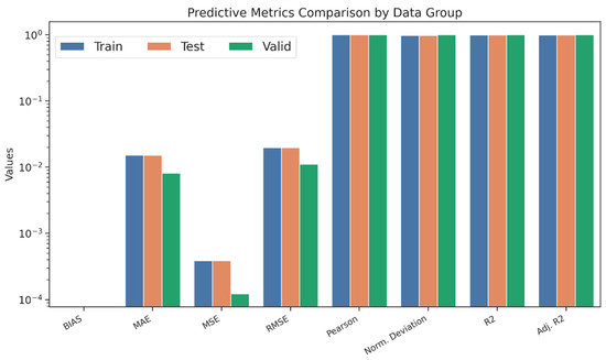
Figure 13.
Comparison of the metrics by dataset.
To support governance auditing, all preprocessing steps, feature transformations, and modeling decisions were fully documented in a structured pipeline. This included explicit data lineage from raw AHS and WDI sources to the harmonized dataset described in Section 3.3, as well as metadata regarding imputation, scaling, and hyperparameter optimization. An audit trail was generated to enable external replication and regulatory compliance, in line with best practices from the Basel Committee on Banking Supervision and the EU AI Act.
Finally, the auditing protocol incorporated drift monitoring and explainability safeguards to ensure ongoing accountability. By embedding governance-aware interpretation directly into the modeling workflow, RECIR advances beyond conventional predictive models to provide interpretable, auditable, and legally compatible outputs. This integration addresses the reviewer’s concern regarding transparency and reproducibility, while reinforcing the framework’s applicability to high-stakes real estate investment decision-making.
4. Findings
4.1. Final Model Selection
Following the extensive benchmarking of eight candidate families, three estimators emerged as consistently dominant: Lars Regression, Decision Tree Regression (DTRg), and Histogram Gradient Boosting Regression (HGBRg). Table 15 summarizes their performance statistics, highlighting differences in accuracy, stability, and computational efficiency. While Lars demonstrated exceptionally high R2 values and low error rates, its linear structure limited its capacity to capture the nonlinear interactions evident in the integrated AHS–WDI–TRS dataset. DTRg offered competitive predictive performance and interpretability but showed greater sensitivity to fluctuations in the data, as reflected in higher variability across folds. In contrast, HGBRg provided the most balanced solution, combining superior accuracy, robust generalization, and the ability to model complex feature interactions with consistently low variance across validation folds. Although HGBRg imposed higher computational costs, this trade-off was considered acceptable considering the governance-sensitive application domain, where consistency and reliability outweigh marginal efficiency gains. The final model was therefore specified as HGBRg with max_iter = 300, learning_rate = 0.1, and min_samples_leaf = 20, a configuration that offered the strongest balance between predictive strength and computational feasibility for risk-sensitive deployment.
Table 15.
Summary statistics of the best estimators for each model.
4.2. Performance
The selected HGBRg model was evaluated on training, testing, and independent validation subsets, with the full set of results reported in Table 16 and Figure 13. Across all partitions, the model achieved R2 and adjusted R2 values consistently above 0.996, with validation performance approaching 0.999, thereby confirming its strong capacity for temporal and out-of-sample generalization. Error measures remained uniformly low, with mean absolute error (MAE) below 0.009 and root mean squared error (RMSE) below 0.02 across training and testing and further reduced to approximately 0.011 in the validation sample. Bias values were close to zero, and Pearson correlation coefficients consistently exceeded 0.99, as depicted in Figure 14, confirming both accuracy and alignment between predictions and observed outcomes.
Table 16.
Comparison of the metrics by dataset.
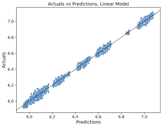
Figure 14.
Actual target values vs. predictions for the selected linear model.
An additional finding concerned the discretized structure of predictions. The TRS, although modeled as a continuous outcome, produced predicted values clustered around discrete risk strata (e.g., 6.06, 6.25, 6.45, and 6.64). Table 17 demonstrates that predicted group means remained nearly identical to actual means, with standard deviations typically below 0.05. This structural fidelity is particularly relevant for decision-making frameworks that rely on risk brackets or threshold-based governance triggers, since it indicates that the model internalizes and reproduces the categorical logic embedded in the TRS. Moreover, the consistency of these results across household-, regional-, and time-level contexts reinforces the applicability of the RECIR framework for both ex ante risk assessment and scenario-based stress testing.
Table 17.
Mean and standard deviation of the actual and prediction groups.
4.3. Baselines & Temporal Generalization
To assess robustness, the RECIR framework was benchmarked against two baselines: a hedonic linear model using standard housing attributes and a macro-only model restricted to aggregate indicators. In both cases, predictive accuracy was markedly lower than that of the integrated HGBRg framework, underscoring the value of combining micro-level AHS variables, macro-level WDI, and governance-salient TRS indices. Temporal generalization was evaluated by training models on the 2015–2019 subsample and testing in 2021–2023, as well as by conducting leave-one-year-out cross-validation. The results confirmed that validation and test R2 closely tracked training performance with only marginal generalization gaps. Ensemble methods, particularly HGBRg, further reduced error variance relative to both linear and tree-based baselines, demonstrating stability in the face of distributional shifts across time.
4.4. Ablation & Parsimony
Ablation tests were conducted to examine the effect of dimensionality reduction on predictive accuracy. The bottom 25%, 50%, and 75% of predictors ranked by validation-set permutation importance were sequentially removed, and models were re-estimated under identical tuning protocols. The removal of the lowest 25% or 50% of features resulted in a median R2 decline of no more than 2–5%, albeit with increased variance across folds. However, eliminating 75% of predictors produced a sharp deterioration in both accuracy and temporal stability. On this basis, two model specifications were retained: a compact top-k model that achieved at least 95% of the baseline accuracy and a full model that maintained superior stability across temporal splits. The monotonic degradation observed in stepwise ablation confirmed that redundancy buffers exist within the dataset but also emphasized the importance of preserving a sufficiently broad feature set to maintain generalizability. This balance between parsimony and robustness strengthens the interpretability of RECIR while ensuring that the model remains practically deployable across diverse governance-sensitive applications.
4.5. Predictive Accuracy
The residual analysis provides strong evidence for the predictive reliability of the final HGBRg model. As illustrated in Figure 15 and summarized in Table 18, the residuals exhibit a symmetric, zero-centered distribution, with more than 90% of values falling between −0.009 and +0.023. This stability across both training and validation partitions confirms the absence of systematic bias. The Q–Q plot (Figure 16) further demonstrates near-perfect alignment with the normal distribution, with only minor deviations at the tails. These results confirm that the residuals satisfy the assumption of normality, thereby supporting the validity of subsequent inference and model reliability.
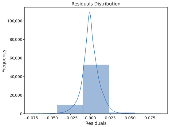
Figure 15.
Histogram of the residuals (actual prediction).
Table 18.
Bins and histogram values of the distribution of the residuals.
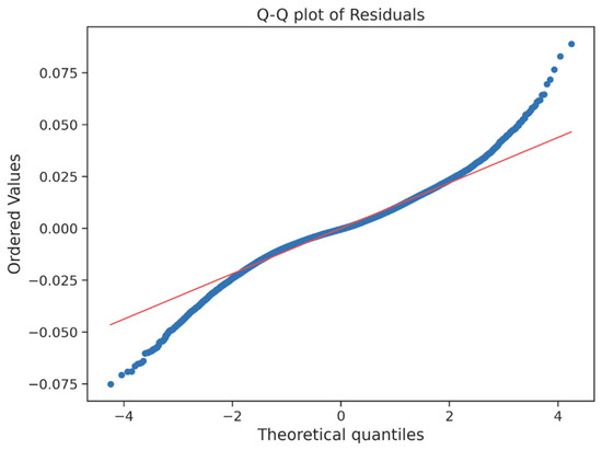
Figure 16.
Quantile–quantile plot of the residuals.
Descriptive statistics reported in Table 19 reinforce this observation: the residual mean approximates zero, the standard deviation remains near 0.011, and skewness and kurtosis are negligible. Aggregate residual metrics (Table 20) confirm minimal prediction errors, with MAE = 0.008, RMSE = 0.011, and bias close to zero. Figure 17 shows residuals plotted against predictions, revealing a uniform scatter with no visible heteroscedasticity, while Table 21 confirms that group-level deviations remain below 1.5 × 10⁻⁴. The variability boundaries reported in Table 22 and the compact box plot in Figure 18 underscore the absence of outliers and validate the model’s robustness. Collectively, these findings confirm that the HGBRg framework achieves both high accuracy and predictive stability, supporting its deployment in operational and policy-relevant settings.
Table 19.
Descriptive statistics of the values of the Q–Q plot.
Table 20.
Statistics and metrics of the residuals.
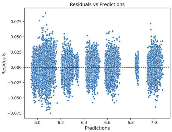
Figure 17.
Residuals and predictions of the selected linear model.
Table 21.
Mean and standard deviation of the residuals and predictions.
Table 22.
Statistics and boundaries of the variability of the residuals.
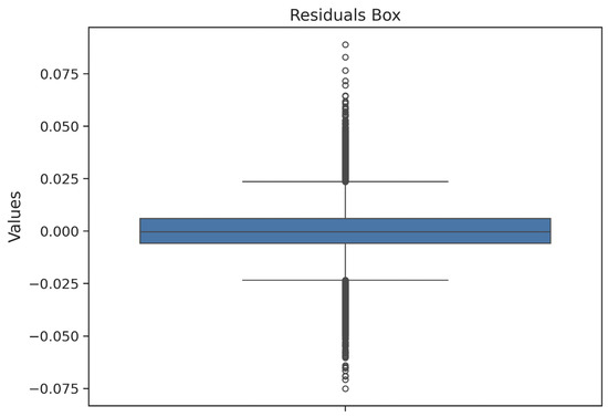
Figure 18.
Box plot of the residuals for the validation set.
Table 19 presents the descriptive statistics of the Q–Q plot values, confirming that the residuals closely follow the theoretical normal distribution.
Table 20 presents the aggregate residual metrics: MAE = 8.07 × 10⁻³, RMSE = 1.11 × 10⁻², and negligible bias. These metrics indicate that the prediction errors are minimal and centered, with no systematic deviation.
Figure 17 plots the residuals against the predicted values and shows a uniform scatter with no discernible pattern or heteroscedasticity. The residuals by prediction group (Table 21) remain below 1.5 × 10⁻⁴, and the standard deviations range from 9.5 × 10⁻³ to 1.4 × 10⁻². These results suggest that prediction uncertainty is minimal and evenly distributed across the output range, thereby supporting the validity and robustness of the model.
No residuals exceed ±4.41 × 10⁻², as defined by the variability thresholds in Table 22.
The box plot of residuals in Figure 18 confirms the symmetry and compactness, with a median centered at zero and the interquartile range tightly constrained. No outliers or anomalous deviations are observed.
4.6. Computational Efficiency and Feature Importance
In addition to accuracy, computational efficiency and feature reliance were evaluated to ensure that RECIR remains practical for real-world deployment. Permutation importance, computed over ten validation repetitions, revealed that predictive influence is concentrated within a small subset of features (Figure 19 and Table 23). Variables such as GASAMT_cat and GASAMT_num each contributed more than 2.3% to model performance, with an additional group of thirteen features—including housing condition, utility costs, and socioeconomic indicators—exerting moderate but consistent influence. Collectively, these variables accounted for nearly 16% of the model’s explanatory power and aligned with the TRS risk domain logic. By contrast, over 70% of features contributed to marginal or negligible effects, with a few exhibiting slightly negative importance because of redundancy or noise.
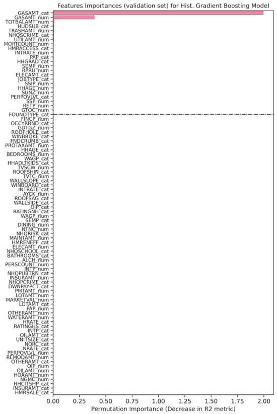
Figure 19.
Permutation importance of the features for the linear model with the best estimator. Bars represent the decrease in R2 when individual features are permuted, thereby quantifying their relative predictive contribution. The dash–dot horizontal line denotes the baseline reference threshold, serving as a cutoff between features with meaningful explanatory power and those with negligible importance.
Table 23.
Ranking of permutation importance.
Despite this imbalance, dimensionality reduction was deliberately avoided at this stage. Eliminating weakly influential variables risked destabilizing predictive performance, particularly under unseen market conditions. Maintaining the broader feature space supports generalizability and preserves modular adaptability for future applications. Notably, the prominence of GASAMT-related features suggests their proxy role for affordability, thermal efficiency, and infrastructure reliability, dimensions closely tied to project-level investment risk. Verification procedures ruled out label leakage by re-estimating importance with grouped encoders and year-fixed effects, confirming consistent rankings within one standard error. Finally, a structured updating protocol (Figure 20) was defined to integrate new data, retrain models, and benchmark evolving feature contributions, thereby ensuring the framework remains adaptive and trustworthy as economic and housing dynamics evolve.
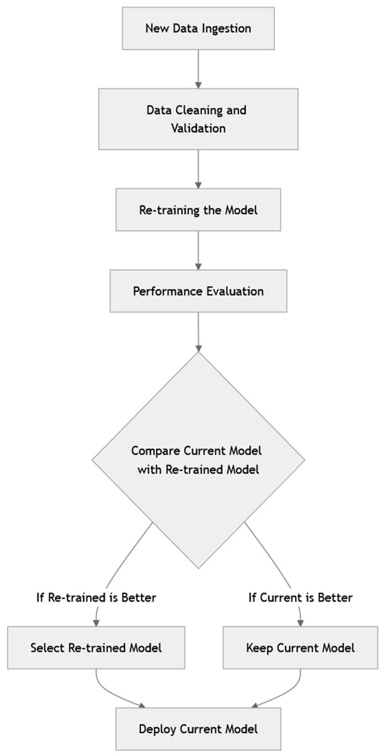
Figure 20.
Model updating plan.
4.7. Discussion and Implications
The findings of this study provide both methodological and substantive contributions to the literature on real estate risk assessment. Methodologically, the RECIR framework advances beyond valuation-centric models by incorporating governance-salient variables, such as permitting and inspection delays, contractor integrity, and regulatory exposures, into a unified, auditable Total Risk Score (TRS). This integration demonstrates that risk assessment cannot be confined to market volatility or macroeconomic indicators alone; rather, it requires a multi-dimensional perspective that captures both structural and institutional determinants of investment outcomes. By achieving consistently high predictive accuracy while maintaining interpretability through permutation importance and cross-validation diagnostics, RECIR contributes to ongoing debates on how to balance complexity and transparency in applied machine learning.
From a theoretical standpoint, the model reframes construction-phase investment risk as a multi-domain construct situated at the intersection of economics, law, and governance. This reconceptualization expands the analytical scope of real estate finance research, which has historically emphasized price forecasting, by embedding regulatory compliance, forensic risk evaluation, and explainability as first-class components of the analytical process. The framework’s macro-to-micro translation mechanism, which links aggregate indicators from the World Development Indicators to unit-level estimates from the American Housing Survey, provides a novel methodological pathway for aligning systemic conditions with granular investment decisions.
Practically, the model’s robustness across temporal splits and its validation against baseline comparators suggest immediate utility for lenders, developers, and policymakers. Financial institutions can apply the TRS in underwriting and portfolio risk management, while regulators may use it as a diagnostic tool to monitor systemic vulnerabilities. The explainability of the outputs further enhances accountability, allowing stakeholders to trace predictions back to legally meaningful variables, which is critical in governance-sensitive contexts such as urban renewal projects or cross-border investment transactions.
Finally, the study addresses broader debates in AI governance by illustrating that high-performing models can remain auditable, interpretable, and compliant with emerging legal frameworks such as the EU AI Act. In this way, RECIR contributes not only to the advancement of real estate risk management but also to the responsible deployment of AI in high-stakes financial domains. Permutation-based feature importance analysis highlights GASAMT_cat as a dominant predictor. This reflects aggregate financing obligations across construction phases, serving as a proxy for liquidity pressure and default risk.
Finally, Figure 20 presents the model updating plan for future iterations. It specifies the procedures for integrating new data, retraining, performance benchmarking, and periodically reassessing the contributions of the feature. This plan ensures that the model remains adaptive and trustworthy because economic and housing dynamics evolve.
5. Conclusions and Future Research Directions
This study introduced the RECIR model as a next-generation framework for evaluating real estate investment risk, designed to integrate micro-level housing data, macroeconomic indicators, and governance-salient regulatory factors into a unified AI-based risk assessment architecture. By combining advanced machine learning algorithms, explainable AI techniques, and regulatory alignment mechanisms, the RECIR significantly enhances predictive accuracy, interpretability, and adaptability relative to traditional econometric approaches. Comparative evidence across Table 10, Table 11, Table 12, Table 13, Table 14 and Table 15 and the summary in Table 24 demonstrates that the model not only reduces forecast error but also provides superior transparency and resilience, thereby offering a methodological contribution to both academic research and professional practice.
Table 24.
Comparison of the RECIR with traditional risk assessment models.
A central strength of the RECIR lies in its ability to incorporate unstructured and high-frequency data sources—including IoT-based property monitoring, real-time financial indicators, and natural language processing of legal documentation—while maintaining alignment with regulatory standards such as the GDPR, the AI Act, and the U.S. Fair Housing Act. This capacity ensures that the model remains operationally scalable and legally defensible, addressing one of the main criticisms in the editor’s review regarding the gap between predictive performance and regulatory compliance. Furthermore, the integration of forensic AI techniques enables early detection of anomalies and fraud, reinforcing the model’s contribution to governance and investor protection.
Despite these advancements, several limitations remain and must be acknowledged explicitly. First, although the RECIR reduces reliance on historical data, the model’s performance may still be challenged in highly volatile markets where structural breaks occur. Second, while the inclusion of environmental and legal indices enhances interpretability, the weighting of such variables may vary across jurisdictions, potentially limiting cross-country generalization. Third, as noted by the reviewers, algorithmic transparency remains a practical challenge: even with explainable AI tools, full interpretability is not always attainable when handling complex ensemble models. Recognizing these limitations responds directly to the editorial request for a balanced discussion of constraints.
Future research directions are therefore threefold. Methodologically, advances in reinforcement learning and continuous training in architecture could further strengthen the model’s responsiveness to market shocks. Comparative studies that evaluate the RECIR alongside hybrid econometrics–AI frameworks would provide empirical evidence of its relative efficiency and robustness across contexts. Substantively, future work should examine the socioeconomic consequences of AI-driven risk models, particularly their impact on investment allocation, housing affordability, and market stability. Technologically, expanding integration with blockchain-verified transactions and decentralized edge-computing infrastructures could address both transparency and cybersecurity concerns. These avenues of inquiry ensure that RECIR remains adaptable to emerging data ecosystems and evolving governance requirements. Although benchmark datasets were not used to evaluate RECIR, we acknowledge this as a limitation. Future research should validate the framework against standardized repositories to strengthen generalizability and facilitate comparative evaluation.
In summary, RECIR contributes to academic literature by unifying heterogeneous data sources under AI-driven, regulation-aware architecture and provides actionable tools for practitioners tasked with managing complex, multi-dimensional risks. Its ability to balance predictive power with regulatory compliance positions it as a pioneering framework for real estate finance. Nevertheless, ongoing refinement and critical evaluation remain essential for realizing its full potential. Future research must continue to align technological innovation with ethical, legal, and social considerations to ensure that AI-driven risk models not only improve prediction but also foster transparency, trust, and fairness across global real estate markets.
A limitation of this study is the absence of external benchmark datasets for model validation. Future research should explicitly test RECIR against standardized repositories to strengthen comparability and external validity.
Author Contributions
Conceptualization, A.L.; methodology, A.L.; formal analysis, A.L.; investigation, A.L.; data curation, A.L.; writing—original draft preparation, A.L.; writing—review and editing, A.L., L.C.L.d.R. and N.C.V.; supervision, L.C.L.d.R. and N.C.V.; project administration, L.C.L.d.R. and N.C.V. All authors have read and agreed to the published version of the manuscript.
Funding
This research received no external funding.
Institutional Review Board Statement
This study was approved by the Institutional Review Board of the University of Cordoba. This study was conducted in accordance with the ethical guidelines of the 1964 Declaration of Helsinki, its subsequent amendments, and similar ethical standards.
Informed Consent Statement
All the participants provided oral consent to include their data in the research and development of the model. No identifiable personal details were obtained.
Data Availability Statement
The data supporting the findings of this study are available from the corresponding author upon reasonable request. The data are not publicly available due to privacy and ethical considerations.
Acknowledgments
We thank José María Caridad y Ocerín for his valuable academic guidance and consistent professional support. His mentorship has been crucial for navigating the complexities of assessing real estate investment risk, particularly in conflict-prone regions. We also thank the participants of our focus groups and surveys, whose insights were essential for grounding our risk assessments in practical considerations and for deepening our understanding of investor sentiment in Ukraine and Israel. We give special acknowledgment to the owners of construction companies and consultants whose expertise contributed to a nuanced understanding of the role of geopolitical factors and AI analytics in shaping investment paradigms. We appreciate the dedicated commitment of everyone involved, which enabled the successful execution and dissemination of this research. The process of authoring this study has been both intellectually rewarding and enlightening.
Conflicts of Interest
The authors declare no conflicts of interest.
Abbreviations
The following abbreviations are used in this manuscript:
| ADPs | additional data points |
| AHS | American Housing Survey |
| AI | artificial intelligence |
| CV | cross-validation |
| HUD | Department of Housing and Urban Development |
| MAE | mean absolute error |
| ML | machine learning |
| MSE | mean squared error |
| NLP | natural language processing |
| PUF | public use file |
| TRS | total risk score |
| WDI | World Development Indicators |
Appendix A
Table A1.
Data sources reviewed to find the input features for the RECIR model.
Table A1.
Data sources reviewed to find the input features for the RECIR model.
| Source | Website | Description | Access Date |
|---|---|---|---|
| Zillow | https://www.zillow.com/research/ | Zillow provides various real estate market reports, housing data, and research insights. | Accessed on 13 October 2025 |
| Redfin | https://www.redfin.com/blog/data-center | Redfin’s data center offers housing market trends, reports, and downloadable datasets. | Accessed on 13 October 2025 |
| Realtor.com | https://www.realtor.com/research/ | Realtor.com Research provides market insights, trends, and reports on the US real estate market. | Accessed on 13 October 2025 |
| Federal Housing Finance Agency (FHFA) | https://www.fhfa.gov/DataTools/Downloads/Pages/House-Price-Index.aspx | FHFA offers the House Price Index (HPI) dataset, providing information on housing price trends. | Accessed on 13 October 2025 |
| U.S. Census Bureau | https://www.census.gov/topics/housing/data.html | The U.S. Census Bureau offers various datasets related to housing and demographics. | Accessed on 13 October 2025 |
| National Association of Realtors (NAR) | https://www.nar.realtor/research-and-statistics | NAR provides research and statistics on the real estate market, including home sales and prices. | Accessed on 13 October 2025 |
| CoreLogic | https://www.corelogic.com/ | CoreLogic offers a range of real estate data, including property information, analytics, and market trends. | Accessed on 13 October 2025 |
| Harvard Joint Center for Housing Studies (JCHS) | https://www.jchs.harvard.edu/data | Harvard JCHS provides datasets on housing markets, demographics, and affordability. | Accessed on 13 October 2025 |
| FRED Economic Data (Federal Reserve Bank of St. Louis) | https://fred.stlouisfed.org/ | FRED offers economic data, including housing-related indicators and economic trends. | Accessed on 13 October 2025 |
| Urban Institute—Housing Finance Policy Center | https://www.urban.org/policy-centers/housing-finance-policy-center | Urban Institute provides research and data on housing finance policies. | Accessed on 13 October 2025 |
| HUD via Data.gov | https://www.data.gov/ | Explore datasets related to housing and urban development from various government agencies. | Accessed on 13 October 2025 |
| Trulia | https://www.trulia.com/research/ | Trulia’s research section offers insights and reports on real estate market trends. | Accessed on 13 October 2025 |
| Attom Data Solutions | https://www.attomdata.com/ | Attom Data Solutions provides property data, analytics, and reports for real estate professionals. | Accessed on 13 October 2025 |
| Harvard JCHS—State of the Nation’s Housing | https://www.jchs.harvard.edu/state-nations-housing | Harvard’s JCHS publishes annual reports on the state of the nation’s housing, including comprehensive data. | Accessed on 13 October 2025 |
| World Bank—World Development Indicators (WDI) | https://databank.worldbank.org/source/world-development-indicators/preview/on | WDI is the primary World Bank collection of development indicators, compiled from international sources. | Accessed on 13 October 2025 |
| MLS Databases | Various local MLSs | Local Multiple Listing Services (MLSs) offer property listings, sales, and market trends (access varies by region). | Accessed on 13 October 2025 |
Note: All data sources listed in Table A1 were accessed at various times between January 2024 and October 2025, depending on availability and the stage of model development.
Table A2.
Final selected variables for the AHS data from the raw data.
Table A2.
Final selected variables for the AHS data from the raw data.
| Detail | Topic | Subtopic | Name | Description |
|---|---|---|---|---|
| household | Occupancy and Tenure | Months Occupied | OCCYRRND | Flag indicating unit is typically occupied year-round |
| Structural | Interior Features | BATHEXCLU | Flag indicating the unit’s bathroom facilities are for the exclusive use of the household | |
| BATHROOMS | Number of bathrooms in unit | |||
| BEDROOMS | Number of bedrooms in unit | |||
| DINING | Number of dining rooms in unit | |||
| FOUNDTYPE | Type of foundation | |||
| TOTROOMS | Number of rooms in unit | |||
| UNITSIZE | Unit size (square feet) | |||
| Housing Problems | Structural Problems | FLOORHOLE | Flag indicating floor has holes | |
| FNDCRUMB | Flag indicating foundation has holes, cracks, or crumbling | |||
| PAINTPEEL | Flag indicating interior area of peeling paint larger than 8 x 11 | |||
| ROOFHOLE | Flag indicating roof has holes | |||
| ROOFSAG | Flag indicating roof’s surface sags or is uneven | |||
| ROOFSHIN | Flag indicating roof has missing shingles or other roofing materials | |||
| WALLCRACK | Flag indicating inside walls or ceilings have open holes or cracks | |||
| WALLSIDE | Flag indicating outside walls have missing siding, bricks, or other missing wall materials | |||
| WALLSLOPE | Flag indicating outside walls slope, lean, buckle, or slant | |||
| WINBOARD | Flag indicating windows are boarded up | |||
| WINBROKE | Flag indicating windows are broken | |||
| Demographics | Householder Demographics | HHADLTKIDS | Number of the householder’s unmarried children age 18 and over, living in this unit | |
| HHAGE | Age of householder | |||
| HHCITSHP | U.S. citizenship of householder | |||
| HHGRAD | Educational level of householder | |||
| Income | Total Household Income | FINCP | Family income (past 12 months) | |
| HINCP | Household income (past 12 months) | |||
| Housing Costs | Total Housing Cost | HOAAMT | Monthly homeowners or condominium association amount | |
| INSURAMT | Monthly homeowner or renter insurance amount | |||
| LOTAMT | Monthly lot rent amount | |||
| MORTAMT | Monthly total mortgage amount (all mortgages) | |||
| PROTAXAMT | Monthly property tax amount | |||
| RENT | Monthly rent amount | |||
| TOTHCAMT | Monthly total housing costs | |||
| UTILAMT | Monthly total utility amount | |||
| Utilities | ELECAMT | Monthly electric amount | ||
| GASAMT | Monthly gas amount | |||
| OILAMT | Monthly oil amount | |||
| OTHERAMT | Monthly amount for other fuels | |||
| TRASHAMT | Monthly trash amount | |||
| WATERAMT | Monthly water amount | |||
| Renter Subsidy | HUDSUB | Subsidized renter status and eligibility | ||
| RENTCNTRL | Flag indicating rent is limited by rent control or stabilization | |||
| RENTSUB | Type of rental subsidy or reduction (based on respondent report) | |||
| Affordability | PERPOVLVL | Household income as a percent of poverty threshold (rounded) | ||
| Owner’s Purchase, Value, and Debt | DWNPAYPCT | Down payment percentage | ||
| FIRSTHOME | Flag indicating if first-time home buyer | |||
| HOWBUY | Description of how owner obtained unit | |||
| LEADINSP | Flag indicating lead pipes inspected before purchase | |||
| MARKETVAL | Current market value of unit | |||
| TOTBALAMT | Total remaining debt across all mortgages or similar debts for this unit | |||
| Home Improvement | General | HMRACCESS | Flag indicating home improvements done in last two years to make home more accessible for those with physical limitations | |
| HMRENEFF | Flag indicating home improvements done to make home more energy efficient in last two years | |||
| HMRSALE | Flag indicating home improvements done to get house ready for sale in last two years | |||
| MAINTAMT | Amount of annual routine maintenance costs | |||
| REMODAMT | Total cost of home improvement jobs in last two years | |||
| REMODJOBS | Total number of home improvement jobs in last two years | |||
| Neighborhood Features | General | NORC | Flag indicating respondent thinks the majority of neighbors 55 or older | |
| Ratings | NHQPCRIME | Agree or disagree: this neighborhood has a lot of petty crime | ||
| NHQPUBTRN | Agree or disagree: this neighborhood has good bus, subway, or commuter train service | |||
| NHQRISK | Agree or disagree: this neighborhood is at high risk for floods or other disasters | |||
| NHQSCHOOL | Agree or disagree: this neighborhood has good schools | |||
| NHQSCRIME | Agree or disagree: this neighborhood has a lot of serious crime | |||
| RATINGHS | Rating of unit as a place to live | |||
| RATINGNH | Rating of neighborhood as place to live | |||
| Housing Search | HRATE | Rating of current home | ||
| NRATE | Rating of current neighborhood | |||
| person | Income | Person Income | INTP | Person’s interest, dividends, and net rental income (past 12 months) |
| OIP | Person’s other income (past 12 months) | |||
| PAP | Person’s public assistance income (past 12 months) | |||
| RETP | Person’s retirement income (past 12 months) | |||
| SEMP | Person’s self-employment income (past 12 months) | |||
| SSIP | Person’s Supplemental Security Income (past 12 months) | |||
| SSP | Person’s Social Security income (past 12 months) | |||
| WAGP | Person’s wages or salary income (past 12 months) | |||
| project | Home Improvement | Job Specific | JOBTYPE | Cost of home improvement job |
| mortgage | Mortgage Details | Mortgage Origination | INTRATE | Interest rate of mortgage |
| Current Payment Details | PMTAMT | Amount of mortgage payment | ||
| TAXPMT | Flag indicating property taxes included in mortgage payment | |||
| Refinance | REFI | Flag indicating mortgage is a refinance of previous mortgage |
Table A3.
Final selected variables for the WDI data from the raw data.
Table A3.
Final selected variables for the WDI data from the raw data.
| Detail | Topic | Subtopic | Model Name | Databank Name | Description |
|---|---|---|---|---|---|
| World Development Indicators (WDI) | Economic Policy & Debt | National accounts | NGMK | NY.GDP.MKTP.KN | GDP (constant LCU) |
| NGPK | NY.GDP.PCAP.KN | GDP per capita (constant LCU) | |||
| NGNMK | NY.GNP.MKTP.KN | GNI (constant LCU) | |||
| NGNPK | NY.GNP.PCAP.KN | GNI per capita (constant LCU) | |||
| NTNC | NY.TRF.NCTR.CN | Net secondary income (Net current transfers from abroad) (current LCU) | |||
| NGNC | NY.GSR.NFCY.CN | Net primary income (Net income from abroad) (current LCU) | |||
| NGIC | NY.GNS.ICTR.CN | Gross savings (current LCU) | |||
| NGPC | NY.GNP.PCAP.CN | GNI per capita (current LCU) | |||
| NGTC | NY.GDS.TOTL.CN | Gross domestic savings (current LCU) | |||
| NGDPC | NY.GDP.PCAP.CN | GDP per capita (current LCU) | |||
| NGMCA | NY.GDP.MKTP.CN.AD | GDP: linked series (current LCU) | |||
| NGMC | NY.GDP.MKTP.CN | GDP (current LCU) | |||
| NGNMC | NY.GNP.MKTP.CN | GNI (current LCU) | |||
| NGMKD | NY.GDP.MKTP.KD | GDP (constant 2015 US$) | |||
| NGPKD | NY.GDP.PCAP.KD | GDP per capita (constant 2015 US$) | |||
| NGNMKD | NY.GNP.MKTP.KD | GNI (constant 2015 US$) | |||
| NGNPKD | NY.GNP.PCAP.KD | GNI per capita (constant 2015 US$) | |||
| Environment | Agricultural production | AYCK | AG.YLD.CREL.KG | Cereal yield (kg per hectare) | |
| APCM | AG.PRD.CREL.MT | Cereal production (metric tons) | |||
| ALCH | AG.LND.CREL.HA | Land under cereal production (hectares) | |||
| Financial Sector | Assets | FRLAZ | FD.RES.LIQU.AS.ZS | Bank liquid reserves to bank assets ratio (%) | |
| FBCZ | FB.BNK.CAPA.ZS | Bank capital to assets ratio (%) | |||
| FANZ | FB.AST.NPER.ZS | Bank nonperforming loans to total gross loans (%) | |||
| Health | Population | SPG | SP.POP.GROW | Population growth (annual %) | |
| SPDY | SP.POP.DPND.YG | Age dependency ratio, young (% of working-age population) | |||
| SPDO | SP.POP.DPND.OL | Age dependency ratio, old (% of working-age population) | |||
| SPPODP | SP.POP.DPND | Age dependency ratio (% of working-age population) | |||
| SP6TZ | SP.POP.65UP.TO.ZS | Population ages 65 and above (% of total population) | |||
| SP0TZ | SP.POP.0014.TO.ZS | Population ages 0–14 (% of total population) | |||
| SP1TZ | SP.POP.1564.TO.ZS | Population ages 15–64 (% of total population) | |||
| Infrastructure | Communications | INBP | IT.NET.BBND.P2 | Fixed broadband subscriptions (per 100 people) | |
| IMMP | IT.MLT.MAIN.P2 | Fixed telephone subscriptions (per 100 people) | |||
| IMM | IT.MLT.MAIN | Fixed telephone subscriptions | |||
| INB | IT.NET.BBND | Fixed broadband subscriptions | |||
| ICS | IT.CEL.SETS | Mobile cellular subscriptions | |||
| Technology | TVTMZ | TX.VAL.TECH.MF.ZS | High-technology exports (% of manufactured exports) | ||
| TVTC | TX.VAL.TECH.CD | High-technology exports (current US$) | |||
| Private Sector & Trade | Exports | TVTZW | TX.VAL.TRAN.ZS.WT | Transport services (% of commercial service exports) | |
| TVSCW | TX.VAL.SERV.CD.WT | Commercial service exports (current US$) | |||
| TVAZU | TX.VAL.AGRI.ZS.UN | Agricultural raw materials exports (% of merchandise exports) | |||
| TVFZU | TX.VAL.FUEL.ZS.UN | Fuel exports (% of merchandise exports) | |||
| Public Sector | Conflict & fragility | VIN | VC.IDP.NWDS | Internally displaced persons, new displacement associated with disasters (number of cases) | |
| Defense & arms trade | MMXC | MS.MIL.XPND.CD | Military expenditure (current USD) | ||
| Government finance | GLTGZ | GC.LBL.TOTL.GD.ZS | Net incurrence of liabilities, total (% of GDP) | ||
| GNTC | GC.NLD.TOTL.CN | Net lending (+)/net borrowing (−) (current LCU) | |||
| GDTC | GC.DOD.TOTL.CN | Central government debt, total (current LCU) | |||
| GATGZ | GC.AST.TOTL.GD.ZS | Net acquisition of financial assets (% of GDP) | |||
| GDTGZ | GC.DOD.TOTL.GD.ZS | Central government debt, total (% of GDP) | |||
| GXTGZ | GC.XPN.TOTL.GD.ZS | Expense (% of GDP) | |||
| GTOC | GC.TAX.OTHR.CN | Other taxes (current LCU) | |||
| Policy & institutions | RPRL | RL.PER.RNK.LOWER | Rule of Law: Percentile Rank, Lower Bound of 90% Confidence Interval | ||
| RPRU | RL.PER.RNK.UPPER | Rule of Law: Percentile Rank, Upper Bound of 90% Confidence Interval | |||
| RSE | RL.STD.ERR | Rule of Law: Standard Error | |||
| RQPRU | RQ.PER.RNK.UPPER | Regulatory Quality: Percentile Rank, Upper Bound of 90% Confidence Interval | |||
| RQSE | RQ.STD.ERR | Regulatory Quality: Standard Error | |||
| Social Protection & Labor | Economic activity | SIEFZ | SL.IND.EMPL.FE.ZS | Employment in industry, female (% of female employment) (modeled ILO estimate) | |
| SIEMZ | SL.IND.EMPL.MA.ZS | Employment in industry, male (% of male employment) (modeled ILO estimate) | |||
| SSEMZ | SL.SRV.EMPL.MA.ZS | Employment in services, male (% of male employment) (modeled ILO estimate) | |||
| SGPEK | SL.GDP.PCAP.EM.KD | GDP per person employed (constant 2021 PPP $) | |||
| SSEFZ | SL.SRV.EMPL.FE.ZS | Employment in services, female (% of female employment) (modeled ILO estimate) | |||
| Labor force structure | STCFNZ | SL.TLF.CACT.FM.NE.ZS | Ratio of female to male labor force participation rate (%) (national estimate) | ||
| STCMZ | SL.TLF.CACT.MA.ZS | Labor force participation rate, male (% of male population ages 15+) (modeled ILO estimate) | |||
| STTFZ | SL.TLF.TOTL.FE.ZS | Labor force, female (% of total labor force) | |||
| STAFZ | SL.TLF.ACTI.FE.ZS | Labor force participation rate, female (% of female population ages 15–64) (modeled ILO estimate) | |||
| STA1FZ | SL.TLF.ACTI.1524.FE.ZS | Labor force participation rate for ages 15–24, female (%) (modeled ILO estimate) | |||
| Migration | SPR | SM.POP.REFG | Refugee population by country or territory of asylum | ||
| Unemployment | SUNZ | SL.UEM.NEET.ZS | Share of youth not in education, employment or training, total (% of youth population) | ||
| SUNMZ | SL.UEM.NEET.ME.ZS | Share of youth not in education, employment or training, total (% of youth population) (modeled ILO estimate) | |||
| SUNMAZ | SL.UEM.NEET.MA.ZS | Share of youth not in education, employment or training, male (% of male youth population) | |||
| SUIFZ | SL.UEM.INTM.FE.ZS | Unemployment with intermediate education, female (% of female labor force with intermediate education) | |||
| SUAMZ | SL.UEM.ADVN.MA.ZS | Unemployment with advanced education, male (% of male labor force with advanced education) | |||
| SUAFZ | SL.UEM.ADVN.FE.ZS | Unemployment with advanced education, female (% of female labor force with advanced education) |
Table A4.
Year distribution of the records (households) and feature composition of the final dataset.
Table A4.
Year distribution of the records (households) and feature composition of the final dataset.
| Number Features and Records of Final Dataset by Year | |||
|---|---|---|---|
| Year | No. Features | No. Records | |
| 2015 | 198 | 69,493 | |
| 2017 | 196 | 66,752 | |
| 2019 | 196 | 63,185 | |
| 2021 | 198 | 64,141 | |
| 2023 | 198 | 55,669 | |
| Final Dataset | 198 | 318,240 | |
| SOURCE | of features (variables) | ||
| AHS | 125 | American Housing Survey (US Census Bureau) | |
| WDI | 72 | World Development Indicators (World Bank) | |
| TRS | 1 | Author Survey (Expert Judgment) | |
| TOTAL | 198 | ||
| VARIABLE TYPE | COUNT | OBSERVATION | |
| KEYS | 2 | YEAR, CONTROL | |
| TARGET VARIABLE | 1 | TRS | |
| INDEPENDENT VARIABLES | 197 | See Table 8 | |
| TOTAL VARIABLES | 200 | ||
| CATEGORICAL | 83 | ||
| NUMERICAL | 114 | ||
Table A5.
Basic statistics of the final dataset.
Table A5.
Basic statistics of the final dataset.
| A. Numerical variables | |||||||||||
|---|---|---|---|---|---|---|---|---|---|---|---|
| Name | Count | Mean | Std | Min | 25% | 50% | 75% | Max | Description | Source | |
| TRS_housing | 319,240 | 6.437771 | 0.315361 | 5.908453 | 6.208251 | 6.439217 | 6.626868 | 7.116613 | Total Risk Score | All sources | |
| BEDROOMS_num | 319,240 | 2.672475 | 1.098498 | 0 | 2 | 3 | 3 | 6 | Number of bedrooms in unit | American Housing Survey (US Census Bureau) | |
| DINING_num | 319,240 | 0.497478 | 0.53361 | 0 | 0 | 0 | 1 | 2 | Number of dining rooms in unit | American Housing Survey (US Census Bureau) | |
| TOTROOMS_num | 319,240 | 5.514785 | 1.800217 | 1 | 4 | 5 | 7 | 14 | Number of rooms in unit | American Housing Survey (US Census Bureau) | |
| HHADLTKIDS_num | 277,511 | 0.226287 | 0.555885 | 0 | 0 | 0 | 0 | 8 | Number of the householder’s unmarried children age 18 and over, living in this unit | American Housing Survey (US Census Bureau) | |
| HHAGE_num | 277,511 | 52.76503 | 16.91829 | 15 | 39 | 53 | 66 | 85 | Age of householder | American Housing Survey (US Census Bureau) | |
| FINCP_num | 277,511 | 82,559.62 | 118,481 | −10,000 | 23,000 | 52,000 | 101,000 | 6,405,000 | Family income (past 12 months) | American Housing Survey (US Census Bureau) | |
| HINCP_num | 277,511 | 86,477.3 | 120,651.6 | −10,000 | 24,970 | 56,900 | 108,000 | 6,445,000 | Household income (past 12 months) | American Housing Survey (US Census Bureau) | |
| HOAAMT_num | 312,735 | 27.96784 | 203.9184 | 0 | 0 | 0 | 0 | 25,947 | Monthly homeowners or condominium association amount | American Housing Survey (US Census Bureau) | |
| INSURAMT_num | 277,085 | 69.44089 | 97.46847 | 0 | 0 | 41 | 99 | 959 | Monthly homeowner or renter insurance amount | American Housing Survey (US Census Bureau) | |
| LOTAMT_num | 317,998 | 6.557805 | 103.7443 | 0 | 0 | 0 | 0 | 10,907 | Monthly lot rent amount | American Housing Survey (US Census Bureau) | |
| MORTAMT_num | 318,639 | 424.1185 | 1782.857 | −7988 | 0 | 0 | 485 | 201,207 | Monthly total mortgage amount (all mortgages) | American Housing Survey (US Census Bureau) | |
| PROTAXAMT_num | 319,240 | 172.9731 | 354.179 | 0 | 0 | 0 | 243 | 9031 | Monthly property tax amount | American Housing Survey (US Census Bureau) | |
| RENT_num | 319,240 | 464.1232 | 888.7809 | 0 | 0 | 0 | 730 | 13,100 | Monthly rent amount | American Housing Survey (US Census Bureau) | |
| TOTHCAMT_num | 277,511 | 1512.421 | 2136.725 | 0 | 650 | 1137 | 1866 | 203,093 | Monthly total housing costs | American Housing Survey (US Census Bureau) | |
| UTILAMT_num | 299,106 | 205.3452 | 153.5214 | 0 | 90 | 190 | 290 | 1790 | Monthly total utility amount | American Housing Survey (US Census Bureau) | |
| ELECAMT_num | 294,314 | 114.1421 | 87.61234 | 0 | 60 | 100 | 150 | 750 | Monthly electric amount | American Housing Survey (US Census Bureau) | |
| GASAMT_num | 294,314 | 38.83496 | 56.30936 | 0 | 0 | 20 | 60 | 700 | Monthly gas amount | American Housing Survey (US Census Bureau) | |
| OILAMT_num | 294,299 | 5.228125 | 34.35815 | 0 | 0 | 0 | 0 | 830 | Monthly oil amount | American Housing Survey (US Census Bureau) | |
| OTHERAMT_num | 294,312 | 1.228866 | 10.96232 | 0 | 0 | 0 | 0 | 480 | Monthly amount for other fuels | American Housing Survey (US Census Bureau) | |
| TRASHAMT_num | 299,106 | 20.64897 | 36.80245 | 0 | 2 | 3 | 30 | 670 | Monthly trash amount | American Housing Survey (US Census Bureau) | |
| WATERAMT_num | 299,106 | 30.65193 | 48.31193 | 0 | 2 | 3 | 50 | 500 | Monthly water amount | American Housing Survey (US Census Bureau) | |
| PERPOVLVL_num | 277,511 | 304.4335 | 175.3248 | 1 | 144 | 312 | 502 | 516 | Household income as percent of poverty threshold (rounded) | American Housing Survey (US Census Bureau) | |
| MARKETVAL_num | 319,240 | 228,432.4 | 467,382 | 0 | 0 | 91,040.5 | 307,983.5 | 11,221,977 | Current market value of unit | American Housing Survey (US Census Bureau) | |
| TOTBALAMT_num | 298,407 | 49,999.22 | 153,204.3 | 0 | 0 | 0 | 0 | 13,660,037 | Total remaining debt across all mortgages or similar debts for this unit | American Housing Survey (US Census Bureau) | |
| MAINTAMT_num | 300,613 | 713.9122 | 2396.192 | 0 | 0 | 0 | 526 | 101,031 | Amount of annual routine maintenance costs | American Housing Survey (US Census Bureau) | |
| REMODAMT_num | 319,240 | 3716.94 | 16,144.24 | 0 | 0 | 0 | 600 | 937,900 | Total cost of home improvement jobs in last two years | American Housing Survey (US Census Bureau) | |
| REMODJOBS_num | 319,240 | 0.792191 | 1.743335 | 0 | 0 | 0 | 1 | 28 | Total number of home improvement jobs in last two years | American Housing Survey (US Census Bureau) | |
| RATINGHS_num | 268,544 | 8.284769 | 1.715192 | 1 | 7 | 8 | 10 | 10 | Rating of unit as a place to live | American Housing Survey (US Census Bureau) | |
| RATINGNH_num | 268,026 | 8.197712 | 1.779518 | 1 | 7 | 8 | 10 | 10 | Rating of neighborhood as place to live | American Housing Survey (US Census Bureau) | |
| PERSCOUNT_num | 319,240 | 2.128223 | 1.586905 | 0 | 1 | 2 | 3 | 19 | Number of people in the household | Derived from AHS Data | |
| INTP_num | 277,511 | 4229.273 | 35,880.09 | −10,000 | 0 | 0 | 0 | 4,911,000 | Person’s interest, dividends, and net rental income (past 12 months) | American Housing Survey (US Census Bureau) | |
| OIP_num | 277,511 | 2218.439 | 17,773.16 | 0 | 0 | 0 | 0 | 3,007,500 | Person’s other income (past 12 months) | American Housing Survey (US Census Bureau) | |
| PAP_num | 277,511 | 80.50247 | 809.5531 | 0 | 0 | 0 | 0 | 40,800 | Person’s public assistance income (past 12 months) | American Housing Survey (US Census Bureau) | |
| RETP_num | 277,511 | 4226.844 | 20,710.15 | 0 | 0 | 0 | 0 | 2,396,000 | Person’s retirement income (past 12 months) | American Housing Survey (US Census Bureau) | |
| SEMP_num | 277,511 | 6307.864 | 55,311.02 | −10,000 | 0 | 0 | 0 | 5,786,000 | Person’s selfemployment income (past 12 months) | American Housing Survey (US Census Bureau) | |
| SSIP_num | 277,511 | 455.2386 | 2512.08 | 0 | 0 | 0 | 0 | 92,000 | Person’s Supplemental Security Income (past 12 months) | American Housing Survey (US Census Bureau) | |
| SSP_num | 277,511 | 5342.128 | 11,074.12 | 0 | 0 | 0 | 4000 | 130,000 | Person’s Social Security income (past 12 months) | American Housing Survey (US Census Bureau) | |
| WAGP_num | 277,511 | 63,617.01 | 96,489.19 | 0 | 0 | 36,000 | 90,000 | 3325,000 | Person’s wages or salary income (past 12 months) | American Housing Survey (US Census Bureau) | |
| PROJCOUNT_num | 319,240 | 0.792191 | 1.743335 | 0 | 0 | 0 | 1 | 28 | Number of home improvement projects | Derived from AHS Data | |
| MORTCOUNT_num | 319,240 | 0.32386 | 0.51829 | 0 | 0 | 0 | 1 | 3 | Number of mortgages | Derived from AHS Data | |
| INTRATE_num | 95,576 | 4.13062 | 1.514271 | 0 | 3.221375 | 3.9 | 4.701 | 20.875 | Interest rate of mortgage | American Housing Survey (US Census Bureau) | |
| PMTAMT_num | 95,576 | 1670.083 | 3004.353 | 0 | 793 | 1274 | 1967 | 171,299 | Amount of mortgage payment | American Housing Survey (US Census Bureau) | |
| NGMK_num | 319,240 | 1.97 × 10¹³ | 1.25 × 10¹² | 1.8 × 10¹³ | 1.89 × 10¹³ | 1.99 × 10¹³ | 2.03 × 10¹³ | 2.18 × 10¹³ | GDP (constant LCU) | World Development Indicators (World Bank) | |
| NGPK_num | 319,240 | 60,134.38 | 2903.059 | 56,428.89 | 58,180.91 | 60,763.88 | 61,244.72 | 65,108.65 | GDP per capita (constant LCU) | World Development Indicators (World Bank) | |
| NGNMK_num | 319,240 | 1.99 × 10¹³ | 1.18 × 10¹² | 1.83 × 10¹³ | 1.91 × 10¹³ | 2.01 × 10¹³ | 2.05 × 10¹³ | 2.18 × 10¹³ | GNI (constant LCU) | World Development Indicators (World Bank) | |
| NGNPK_num | 319,240 | 60,725.35 | 2669.867 | 57,320.37 | 58,882.39 | 61,469.96 | 61,648.12 | 65,277.41 | GNI per capita (constant LCU) | World Development Indicators (World Bank) | |
| NTNC_num | 319,240 | −1.3 × 10¹¹ | 2.03 × 10¹⁰ | −1.7 × 10¹¹ | −1.5 × 10¹¹ | −1.3 × 10¹¹ | −1.2 × 10¹¹ | −1.1 × 10¹¹ | Net secondary income (Net current transfers from abroad) (current LCU) | World Development Indicators (World Bank) | |
| NGNC_num | 319,240 | 2.19 × 10¹¹ | 5.59 × 10¹⁰ | 1.25 × 10¹¹ | 1.82 × 10¹¹ | 2.28 × 10¹¹ | 2.62 × 10¹¹ | 2.86 × 10¹¹ | Net primary income (Net income from abroad) (current LCU) | World Development Indicators (World Bank) | |
| NGIC_num | 319,240 | 3.99 × 10¹² | 4.45 × 10¹¹ | 3.53 × 10¹² | 3.61 × 10¹² | 4.07 × 10¹² | 4.08 × 10¹² | 4.82 × 10¹² | Gross savings (current LCU) | World Development Indicators (World Bank) | |
| NGPC_num | 319,240 | 65,622.13 | 7892.876 | 57,251.02 | 59,886.72 | 65,092.35 | 68,249.1 | 80,523.81 | GNI per capita (current LCU) | World Development Indicators (World Bank) | |
| NGTC_num | 319,240 | 3.92 × 10¹² | 5.63 × 10¹¹ | 3.28 × 10¹² | 3.52 × 10¹² | 3.98 × 10¹² | 4.07 × 10¹² | 4.96 × 10¹² | Gross domestic savings (current LCU) | World Development Indicators (World Bank) | |
| NGDPC_num | 319,240 | 65,022.33 | 8181.068 | 56,172.26 | 59,264.44 | 64,402.86 | 67,864.84 | 80,402.29 | GDP per capita (current LCU) | World Development Indicators (World Bank) | |
| NGMCA_num | 319,240 | 2.13 × 10¹³ | 3.01 × 10¹² | 1.8 × 10¹³ | 1.92 × 10¹³ | 2.11 × 10¹³ | 2.25 × 10¹³ | 2.69 × 10¹³ | GDP: linked series (current LCU) | World Development Indicators (World Bank) | |
| NGMC_num | 319,240 | 2.13 × 10¹³ | 3.01 × 10¹² | 1.8 × 10¹³ | 1.92 × 10¹³ | 2.11 × 10¹³ | 2.25 × 10¹³ | 2.69 × 10¹³ | GDP (current LCU) | World Development Indicators (World Bank) | |
| NGNMC_num | 319,240 | 2.15 × 10¹³ | 2.92 × 10¹² | 1.83 × 10¹³ | 1.94 × 10¹³ | 2.13 × 10¹³ | 2.26 × 10¹³ | 2.69 × 10¹³ | GNI (current LCU) | World Development Indicators (World Bank) | |
| NGMKD_num | 319,240 | 1.97 × 10¹³ | 1.25 × 10¹² | 1.8 × 10¹³ | 1.89 × 10¹³ | 1.99 × 10¹³ | 2.03 × 10¹³ | 2.18 × 10¹³ | GDP (constant 2015 US$) | World Development Indicators (World Bank) | |
| NGPKD_num | 319,240 | 60,134.38 | 2903.059 | 56,428.89 | 58,180.91 | 60,763.88 | 61,244.72 | 65,108.65 | GDP per capita (constant 2015 US$) | World Development Indicators (World Bank) | |
| NGNMKD_num | 319,240 | 1.99 × 10¹³ | 1.18 × 10¹² | 1.83 × 10¹³ | 1.91 × 10¹³ | 2.01 × 10¹³ | 2.05 × 10¹³ | 2.18 × 10¹³ | GNI (constant 2015 US$) | World Development Indicators (World Bank) | |
| NGNPKD_num | 319,240 | 60,725.35 | 2669.867 | 57,320.37 | 58,882.39 | 61,469.96 | 61,648.12 | 65,277.41 | GNI per capita (constant 2015 US$) | World Development Indicators (World Bank) | |
| AYCK_num | 319,240 | 8117.029 | 331.1207 | 7534.1 | 8100.75 | 8198.35 | 8372.93 | 8447.75 | Cereal yield (kg per hectare) | World Development Indicators (World Bank) | |
| APCM_num | 319,240 | 4.49 × 100⁸ | 15,843,828 | 4.3 × 100⁸ | 4.37 × 100⁸ | 4.42 × 100⁸ | 4.63 × 100⁸ | 4.72 × 100⁸ | Cereal production (metric tons) | World Development Indicators (World Bank) | |
| ALCH_num | 319,240 | 55,665,136 | 1,904,915 | 53,111,230 | 53,963,016 | 55,805,029 | 57,377,828 | 58,051,885 | Land under cereal production (hectares) | World Development Indicators (World Bank) | |
| FRLAZ_num | 319,240 | 14.68726 | 3.409423 | 9.410917 | 12.53117 | 15.29589 | 17.72731 | 18.8309 | Bank liquid reserves to bank assets ratio (%) | World Development Indicators (World Bank) | |
| FBCZ_num | 319,240 | 9.210828 | 0.302499 | 8.61504 | 9.282331 | 9.355478 | 9.399317 | 9.418105 | Bank capital to assets ratio (%) | World Development Indicators (World Bank) | |
| FANZ_num | 319,240 | 1.248317 | 0.310957 | 0.884207 | 0.939417 | 1.223673 | 1.53055 | 1.662069 | Bank nonperforming loans to total gross loans (%) | World Development Indicators (World Bank) | |
| SPG_num | 319,240 | 0.5871 | 0.112994 | 0.429699 | 0.490908 | 0.563171 | 0.67866 | 0.734789 | Population growth (annual %) | World Development Indicators (World Bank) | |
| SPDY_num | 319,240 | 28.27517 | 0.579775 | 27.25321 | 27.9102 | 28.40665 | 28.69683 | 28.9061 | Age dependency ratio, young (% of workingage population) | World Development Indicators (World Bank) | |
| SPDO_num | 319,240 | 23.54723 | 1.79117 | 21.26373 | 22.31532 | 23.52238 | 24.8605 | 26.39001 | Age dependency ratio, old (% of workingage population) | World Development Indicators (World Bank) | |
| SPPODP_num | 319,240 | 51.82239 | 1.221816 | 50.16983 | 51.01214 | 51.92904 | 52.7707 | 53.64322 | Age dependency ratio (% of workingage population) | World Development Indicators (World Bank) | |
| SP6TZ_num | 319,240 | 15.50098 | 1.053649 | 14.15958 | 14.77693 | 15.48219 | 16.27284 | 17.17572 | Population ages 65 and above (% of total population) | World Development Indicators (World Bank) | |
| SP0TZ_num | 319,240 | 18.62817 | 0.527452 | 17.73823 | 18.26949 | 18.69746 | 19.00309 | 19.24902 | Population ages 0−14 (% of total population) | World Development Indicators (World Bank) | |
| SP1TZ_num | 319,240 | 65.87084 | 0.529827 | 65.08605 | 65.45767 | 65.82036 | 66.21998 | 66.5914 | Population ages 15−64 (% of total population) | World Development Indicators (World Bank) | |
| INBP_num | 319,240 | 33.98047 | 2.540882 | 30.80605 | 32.34235 | 33.44555 | 36.36155 | 37.7711 | Fixed broadband subscriptions (per 100 people) | World Development Indicators (World Bank) | |
| IMMP_num | 319,240 | 32.90733 | 4.462145 | 26.55 | 29.3 | 32.2 | 35.95 | 39.05 | Fixed telephone subscriptions (per 100 people) | World Development Indicators (World Bank) | |
| IMM_num | 319,240 | 1.1 × 100⁸ | 12,763,103 | 90,907,000 | 99,507,000 | 1.08 × 100⁸ | 1.19 × 100⁸ | 1.27 × 100⁸ | Fixed telephone subscriptions | World Development Indicators (World Bank) | |
| INB_num | 319,240 | 1.14 × 100⁸ | 10,674,682 | 99,900,000 | 1.07 × 100⁸ | 1.13 × 100⁸ | 1.24 × 100⁸ | 1.3 × 100⁸ | Fixed broadband subscriptions | World Development Indicators (World Bank) | |
| ICS_num | 319,240 | 3.5 × 100⁸ | 17,301,098 | 3.28 × 100⁸ | 3.39 × 100⁸ | 3.52 × 100⁸ | 3.58 × 100⁸ | 3.8 × 100⁸ | Mobile cellular subscriptions | World Development Indicators (World Bank) | |
| TVTMZ_num | 319,240 | 20.25086 | 0.973616 | 18.58483 | 19.69772 | 20.84263 | 20.93742 | 21.21249 | Hightechnology exports (% of manufactured exports) | World Development Indicators (World Bank) | |
| TVTC_num | 319,240 | 1.69 × 10¹¹ | 1.63 × 10¹⁰ | 1.54 × 10¹¹ | 1.55 × 10¹¹ | 1.64 × 10¹¹ | 1.76 × 10¹¹ | 2 × 10¹¹ | Hightechnology exports (current US$) | World Development Indicators (World Bank) | |
| TVTZW_num | 319,240 | 10.32887 | 1.152628 | 8.350894 | 9.94246 | 10.62805 | 10.76102 | 11.78374 | Transport services (% of commercial service exports) | World Development Indicators (World Bank) | |
| TVSCW_num | 319,240 | 8.13 × 10¹¹ | 7.82 × 10¹⁰ | 7.43 × 10¹¹ | 7.43 × 10¹¹ | 7.91 × 10¹¹ | 8.56 × 10¹¹ | 9.57 × 10¹¹ | Commercial service exports (current US$) | World Development Indicators (World Bank) | |
| TVAZU_num | 319,240 | 2.144748 | 0.143138 | 1.88866 | 2.090265 | 2.123947 | 2.279152 | 2.290435 | Agricultural raw materials exports (% of merchandise exports) | World Development Indicators (World Bank) | |
| TVFZU_num | 319,240 | 13.07431 | 3.884633 | 9.044552 | 9.494549 | 13.86468 | 14.31904 | 20.04383 | Fuel exports (% of merchandise exports) | World Development Indicators (World Bank) | |
| VIN_num | 319,240 | 814,043.8 | 499,162.7 | 48,500 | 438,500 | 1,081,500 | 1,144,000 | 1,354,000 | Internally displaced persons, new displacement associated with disasters (number of cases) | World Development Indicators (World Bank) | |
| MMXC_num | 319,240 | 7.28 × 10¹¹ | 9.24 × 10¹⁰ | 6.41 × 10¹¹ | 6.43 × 10¹¹ | 7.08 × 10¹¹ | 7.92 × 10¹¹ | 8.88 × 10¹¹ | Military expenditure (current USD) | World Development Indicators (World Bank) | |
| GLTGZ_num | 319,240 | 7.128477 | 4.007017 | 3.96595 | 4.237253 | 5.885602 | 7.095942 | 14.8048 | Net incurrence of liabilities, total (% of GDP) | World Development Indicators (World Bank) | |
| GNTC_num | 319,240 | −1.4 × 10¹² | 8.75 × 10¹¹ | −3 × 10¹² | −1.6 × 10¹² | −1.1 × 10¹² | −6.5 × 10¹¹ | −6.2 × 10¹¹ | Net lending (+)/net borrowing (−) (current LCU) | World Development Indicators (World Bank) | |
| GDTC_num | 319,240 | 2.26 × 10¹³ | 5.07 × 10¹² | 1.72 × 10¹³ | 1.87 × 10¹³ | 2.09 × 10¹³ | 2.73 × 10¹³ | 3.06 × 10¹³ | Central government debt, total (current LCU) | World Development Indicators (World Bank) | |
| GATGZ_num | 319,240 | 0.894788 | 0.283848 | 0.596667 | 0.683851 | 0.812949 | 0.952981 | 1.409915 | Net acquisition of financial assets (% of GDP) | World Development Indicators (World Bank) | |
| GDTGZ_num | 319,240 | 105.1277 | 10.27927 | 95.70481 | 97.47495 | 99.24091 | 113.8834 | 121.5008 | Central government debt, total (% of GDP) | World Development Indicators (World Bank) | |
| GXTGZ_num | 319,240 | 24.44842 | 3.44769 | 22.27831 | 22.34298 | 22.4918 | 24.09891 | 31.20412 | Expense (% of GDP) | World Development Indicators (World Bank) | |
| GTOC_num | 319,240 | 4.71 × 10¹⁰ | 4.7 × 10¹⁰ | 1.94 × 10¹⁰ | 1.95 × 10¹⁰ | 2.32 × 10¹⁰ | 3.14 × 10¹⁰ | 1.38 × 10¹¹ | Other taxes (current LCU) | World Development Indicators (World Bank) | |
| RPRL_num | 319,240 | 85.35579 | 1.621815 | 83.01887 | 83.80952 | 85.47619 | 86.60028 | 87.38095 | Rule of Law: Percentile Rank, Lower Bound of 90% Confidence Interval | World Development Indicators (World Bank) | |
| RPRU_num | 319,240 | 94.46973 | 1.89013 | 92.38095 | 92.92453 | 93.80952 | 95.21062 | 97.61905 | Rule of Law: Percentile Rank, Upper Bound of 90% Confidence Interval | World Development Indicators (World Bank) | |
| RSE_num | 319,240 | 0.160035 | 0.005182 | 0.15412 | 0.154673 | 0.160141 | 0.164199 | 0.167804 | Rule of Law: Standard Error | World Development Indicators (World Bank) | |
| RQPRU_num | 319,240 | 95.97601 | 1.834019 | 92.58471 | 96.42857 | 96.66667 | 96.93396 | 97.61905 | Regulatory Quality: Percentile Rank, Upper Bound of 90% Confidence Interval | World Development Indicators (World Bank) | |
| RQSE_num | 319,240 | 0.227125 | 0.005551 | 0.221328 | 0.223406 | 0.224027 | 0.232495 | 0.235875 | Regulatory Quality: Standard Error | World Development Indicators (World Bank) | |
| SIEFZ_num | 319,240 | 8.527767 | 0.060608 | 8.423692 | 8.519016 | 8.531087 | 8.575221 | 8.599635 | Employment in industry, female (% of female employment) (modeled ILO estimate) | World Development Indicators (World Bank) | |
| SIEMZ_num | 319,240 | 28.48904 | 0.234365 | 28.1772 | 28.24099 | 28.51357 | 28.71592 | 28.74575 | Employment in industry, male (% of male employment) (modeled ILO estimate) | World Development Indicators (World Bank) | |
| SSEMZ_num | 319,240 | 69.20172 | 0.315729 | 68.86961 | 68.98205 | 69.04037 | 69.54918 | 69.65875 | Employment in services, male (% of male employment) (modeled ILO estimate) | World Development Indicators (World Bank) | |
| SGPEK_num | 319,240 | 141,434.3 | 6084.95 | 134,569.2 | 136,422.9 | 140,202.3 | 147,749.9 | 150,135.2 | GDP per person employed (constant 2021 PPP $) | World Development Indicators (World Bank) | |
| SSEFZ_num | 319,240 | 90.50678 | 0.067141 | 90.4108 | 90.46812 | 90.50777 | 90.5118 | 90.6182 | Employment in services, female (% of female employment) (modeled ILO estimate) | World Development Indicators (World Bank) | |
| STCFNZ_num | 319,240 | 82.81009 | 0.573211 | 82.19841 | 82.33613 | 82.85047 | 83.01751 | 83.85717 | Ratio of female to male labor force participation rate (%) (national estimate) | World Development Indicators (World Bank) | |
| STCMZ_num | 319,240 | 68.25799 | 0.622571 | 67.3775 | 67.5515 | 68.696 | 68.7545 | 68.768 | Labor force participation rate, male (% of male population ages 15+) (modeled ILO estimate) | World Development Indicators (World Bank) | |
| STTFZ_num | 319,240 | 45.19341 | 0.118051 | 45.07938 | 45.13319 | 45.16603 | 45.19355 | 45.4362 | Labor force, female (% of total labor force) | World Development Indicators (World Bank) | |
| STAFZ_num | 319,240 | 66.85501 | 0.799545 | 65.8365 | 66.404 | 66.7935 | 67.3005 | 68.2325 | Labor force participation rate, female (% of female population ages 15–64) (modeled ILO estimate) | World Development Indicators (World Bank) | |
| STA1FZ_num | 319,240 | 49.36338 | 0.544539 | 48.807 | 48.972 | 49.115 | 49.849 | 50.2555 | Labor force participation rate for ages 15–24, female (%) (modeled ILO estimate) | World Development Indicators (World Bank) | |
| SPR_num | 319,240 | 317,840 | 41,508.42 | 270,206 | 280,049 | 327,478.5 | 340,012.5 | 386,130.5 | Refugee population by country or territory of asylum | World Development Indicators (World Bank) | |
| SUNZ_num | 319,240 | 11.90356 | 0.952111 | 10.6655 | 11.2175 | 11.4945 | 12.915 | 13.0485 | Share of youth not in education, employment or training, total (% of youth population) | World Development Indicators (World Bank) | |
| SUNMZ_num | 319,240 | 11.90356 | 0.952111 | 10.6655 | 11.2175 | 11.4945 | 12.915 | 13.0485 | Share of youth not in education, employment or training, total (% of youth population) (modeled ILO estimate) | World Development Indicators (World Bank) | |
| SUNMAZ_num | 319,240 | 11.28533 | 0.930138 | 10.0995 | 10.714 | 10.8815 | 11.9375 | 12.692 | Share of youth not in education, employment or training, male (% of male youth population) | World Development Indicators (World Bank) | |
| SUIFZ_num | 319,240 | 6.56709 | 1.561493 | 4.9295 | 5.007 | 6.069 | 7.462 | 9.074 | Unemployment with intermediate education, female (% of female labor force with intermediate education) | World Development Indicators (World Bank) | |
| SUAMZ_num | 319,240 | 3.039129 | 0.747095 | 2.375 | 2.382 | 2.7155 | 3.2345 | 4.388 | Unemployment with advanced education, male (% of male labor force with advanced education) | World Development Indicators (World Bank) | |
| SUAFZ_num | 319,240 | 3.207142 | 0.88418 | 2.32 | 2.447 | 2.876 | 3.485 | 4.7695 | Unemployment with advanced education, female (% of female labor force with advanced education) | World Development Indicators (World Bank) | |
| B. Categorical variables | |||||||||||
| Name | Count | Unique | Top | Freq | Unique Values | Mode | Description | Source | |||
| OCCYRRND_cat | 318,269 | 3 | −6 | 277,511 | 3 | −6 | Flag indicating unit is typically occupied yearround (category) | American Housing Survey (US Census Bureau) | |||
| BATHEXCLU_cat | 319,211 | 3 | −6 | 318,636 | 3 | −6 | Flag indicating the unit’s bathroom facilities are for the exclusive use of the household (category) | American Housing Survey (US Census Bureau) | |||
| BATHROOMS_cat | 319,240 | 13 | 1 | 114,275 | 13 | 1 | Number of bathrooms in unit (category) | American Housing Survey (US Census Bureau) | |||
| FOUNDTYPE_cat | 319,240 | 10 | −6 | 98,917 | 10 | −6 | Type of foundation (category) | American Housing Survey (US Census Bureau) | |||
| UNITSIZE_cat | 277,430 | 9 | 4 | 70,560 | 9 | 4 | Unit size (square feet) (category) | American Housing Survey (US Census Bureau) | |||
| FLOORHOLE_cat | 319,240 | 2 | 2 | 313,454 | 2 | 2 | Flag indicating floor has holes (category) | American Housing Survey (US Census Bureau) | |||
| FNDCRUMB_cat | 311,751 | 3 | 2 | 200,118 | 3 | 2 | Flag indicating foundation has holes, cracks, or crumbling (category) | American Housing Survey (US Census Bureau) | |||
| PAINTPEEL_cat | 319,240 | 2 | 2 | 310,836 | 2 | 2 | Flag indicating interior area of peeling paint larger than 8 × 11 (category) | American Housing Survey (US Census Bureau) | |||
| ROOFHOLE_cat | 312,352 | 3 | 2 | 209,246 | 3 | 2 | Flag indicating roof has holes (category) | American Housing Survey (US Census Bureau) | |||
| ROOFSAG_cat | 312,981 | 3 | 2 | 208,810 | 3 | 2 | Flag indicating roof’s surface sags or is uneven (category) | American Housing Survey (US Census Bureau) | |||
| ROOFSHIN_cat | 312,387 | 3 | 2 | 205,005 | 3 | 2 | Flag indicating roof has missing shingles or other roofing materials (category) | American Housing Survey (US Census Bureau) | |||
| WALLCRACK_cat | 319,240 | 2 | 2 | 300,075 | 2 | 2 | Flag indicating inside walls or ceilings have open holes or cracks (category) | American Housing Survey (US Census Bureau) | |||
| WALLSIDE_cat | 313,503 | 3 | 2 | 207,868 | 3 | 2 | Flag indicating outside walls have missing siding, bricks, or other missing wall materials (category) | American Housing Survey (US Census Bureau) | |||
| WALLSLOPE_cat | 313,645 | 3 | 2 | 211,228 | 3 | 2 | Flag indicating outside walls slope, lean, buckle, or slant (category) | American Housing Survey (US Census Bureau) | |||
| WINBOARD_cat | 314,626 | 3 | 2 | 211,668 | 3 | 2 | Flag indicating windows are boarded up (category) | American Housing Survey (US Census Bureau) | |||
| WINBROKE_cat | 314,380 | 3 | 2 | 205,750 | 3 | 2 | Flag indicating windows are broken (category) | American Housing Survey (US Census Bureau) | |||
| HHADLTKIDS_cat | 319,240 | 2 | 0 | 277,511 | 2 | 0 | Number of the householder’s unmarried children age 18 and over, living in this unit (category) | American Housing Survey (US Census Bureau) | |||
| HHAGE_cat | 319,240 | 3 | 0 | 267,972 | 3 | 0 | Age of householder (category) | American Housing Survey (US Census Bureau) | |||
| HHCITSHP_cat | 319,240 | 6 | 1 | 220,318 | 6 | 1 | U.S. citizenship of householder (category) | American Housing Survey (US Census Bureau) | |||
| HHGRAD_cat | 319,240 | 18 | 39 | 65,875 | 18 | 39 | Educational level of householder (category) | American Housing Survey (US Census Bureau) | |||
| FINCP_cat | 319,240 | 2 | −1 × 10⁸ | 277,511 | 2 | −1 × 10⁸ | Family income (past 12 months) (category) | American Housing Survey (US Census Bureau) | |||
| HINCP_cat | 319,240 | 2 | −1 × 10⁸ | 277,511 | 2 | −1 × 10⁸ | Household income (past 12 months) (category) | American Housing Survey (US Census Bureau) | |||
| HOAAMT_cat | 312,735 | 2 | 0 | 165,946 | 2 | 0 | Monthly homeowners or condominium association amount (category) | American Housing Survey (US Census Bureau) | |||
| INSURAMT_amax | 277,085 | 2 | 0 | 276,750 | 2 | 0 | Monthly homeowner or renter insurance amount (topcoded) | American Housing Survey (US Census Bureau) | |||
| INSURAMT_cat | 318,814 | 3 | 0 | 276,750 | 3 | 0 | Monthly homeowner or renter insurance amount (category) | American Housing Survey (US Census Bureau) | |||
| LOTAMT_amax | 7462 | 2 | 0 | 7457 | 2 | 0 | Monthly lot rent amount (topcoded) | American Housing Survey (US Census Bureau) | |||
| LOTAMT_cat | 317,998 | 4 | −6 | 310,536 | 4 | −6 | Monthly lot rent amount (category) | American Housing Survey (US Census Bureau) | |||
| MORTAMT_cat | 318,639 | 2 | −6 | 223,664 | 2 | −6 | Monthly total mortgage amount (all mortgages) (category) | American Housing Survey (US Census Bureau) | |||
| PROTAXAMT_amax | 163,984 | 2 | 0 | 163,936 | 2 | 0 | Monthly property tax amount (topcoded) | American Housing Survey (US Census Bureau) | |||
| PROTAXAMT_cat | 319,240 | 3 | 0 | 163,936 | 3 | 0 | Monthly property tax amount (category) | American Housing Survey (US Census Bureau) | |||
| RENT_cat | 319,240 | 3 | −6 | 191,994 | 3 | −6 | Monthly rent amount (category) | American Housing Survey (US Census Bureau) | |||
| TOTHCAMT_cat | 319,240 | 2 | 0 | 277,511 | 2 | 0 | Monthly total housing costs (category) | American Housing Survey (US Census Bureau) | |||
| UTILAMT_cat | 319,240 | 3 | 1 | 262,682 | 3 | 1 | Monthly total utility amount (category) | American Housing Survey (US Census Bureau) | |||
| ELECAMT_cat | 319,240 | 6 | 4 | 260,096 | 6 | 4 | Monthly electric amount (category) | American Housing Survey (US Census Bureau) | |||
| GASAMT_cat | 319,240 | 6 | 4 | 167,729 | 6 | 4 | Monthly gas amount (category) | American Housing Survey (US Census Bureau) | |||
| OILAMT_cat | 319,225 | 6 | 0 | 276,672 | 6 | 0 | Monthly oil amount (category) | American Housing Survey (US Census Bureau) | |||
| OTHERAMT_cat | 319,238 | 6 | 0 | 274,024 | 6 | 0 | Monthly amount for other fuels (category) | American Housing Survey (US Census Bureau) | |||
| TRASHAMT_cat | 319,240 | 6 | 4 | 128,957 | 6 | 4 | Monthly trash amount (category) | American Housing Survey (US Census Bureau) | |||
| WATERAMT_cat | 319,240 | 6 | 4 | 133,897 | 6 | 4 | Monthly water amount (category) | American Housing Survey (US Census Bureau) | |||
| HUDSUB_cat | 319,240 | 4 | −6 | 204,395 | 4 | −6 | Subsidized renter status and eligibility (category) | American Housing Survey (US Census Bureau) | |||
| RENTCNTRL_cat | 317,904 | 3 | −6 | 300,622 | 3 | −6 | Flag indicating rent is limited by rent control or stabilization (category) | American Housing Survey (US Census Bureau) | |||
| RENTSUB_cat | 315,889 | 9 | −6 | 188,233 | 9 | −6 | Type of rental subsidy or reduction (based on respondent report) (category) | American Housing Survey (US Census Bureau) | |||
| PERPOVLVL_amax | 277,511 | 2 | 0 | 194,729 | 2 | 0 | Household income as percent of poverty threshold (rounded) (topcoded) | American Housing Survey (US Census Bureau) | |||
| PERPOVLVL_cat | 319,240 | 4 | 2 | 188,075 | 4 | 2 | Household income as percent of poverty threshold (rounded) (category) | American Housing Survey (US Census Bureau) | |||
| DWNPAYPCT_cat | 289,122 | 11 | −6 | 171,179 | 11 | −6 | Down payment percentage (category) | American Housing Survey (US Census Bureau) | |||
| FIRSTHOME_cat | 312,037 | 3 | −6 | 156,574 | 3 | −6 | Flag indicating if firsttime home buyer (category) | American Housing Survey (US Census Bureau) | |||
| HOWBUY_cat | 314,839 | 6 | −6 | 156,574 | 6 | −6 | Description of how owner obtained unit (category) | American Housing Survey (US Census Bureau) | |||
| LEADINSP_cat | 310,303 | 3 | −6 | 156,574 | 3 | −6 | Flag indicating lead pipes inspected before purchase (category) | American Housing Survey (US Census Bureau) | |||
| MARKETVAL_amax | 188,233 | 2 | 0 | 188,134 | 2 | 0 | Current market value of unit (topcoded) | American Housing Survey (US Census Bureau) | |||
| MARKETVAL_cat | 319,240 | 3 | 1 | 188,134 | 3 | 1 | Current market value of unit (category) | American Housing Survey (US Census Bureau) | |||
| TOTBALAMT_cat | 298,407 | 2 | −6 | 223,664 | 2 | −6 | Total remaining debt across all mortgages or similar debts for this unit (category) | American Housing Survey (US Census Bureau) | |||
| HMRACCESS_cat | 318,960 | 3 | −6 | 225,695 | 3 | −6 | Flag indicating home improvements done in last two years to make home more accessible for those with physical limitations (category) | American Housing Survey (US Census Bureau) | |||
| HMRENEFF_cat | 318,878 | 3 | −6 | 225,695 | 3 | −6 | Flag indicating home improvements done to make home more energy efficient in last two years (category) | American Housing Survey (US Census Bureau) | |||
| HMRSALE_cat | 318,947 | 3 | −6 | 225,695 | 3 | −6 | Flag indicating home improvements done to get house ready for sale in last two years (category) | American Housing Survey (US Census Bureau) | |||
| MAINTAMT_amax | 144,039 | 2 | 0 | 144,038 | 2 | 0 | Amount of annual routine maintenance costs (topcoded) | American Housing Survey (US Census Bureau) | |||
| MAINTAMT_cat | 300,613 | 3 | −6 | 156,574 | 3 | −6 | Amount of annual routine maintenance costs (category) | American Housing Survey (US Census Bureau) | |||
| REMODAMT_cat | 319,240 | 2 | 0 | 162,666 | 2 | 0 | Total cost of home improvement jobs in last two years (category) | American Housing Survey (US Census Bureau) | |||
| REMODJOBS_cat | 319,240 | 2 | 0 | 162,666 | 2 | 0 | Total number of home improvement jobs in last two years (category) | American Housing Survey (US Census Bureau) | |||
| NORC_cat | 313,978 | 3 | −6 | 256,048 | 3 | −6 | Flag indicating respondent thinks the majority of neighbors 55 or older (category) | American Housing Survey (US Census Bureau) | |||
| NHQPCRIME_cat | 305,254 | 3 | 2 | 219,292 | 3 | 2 | Agree or disagree: this neighborhood has a lot of petty crime (category) | American Housing Survey (US Census Bureau) | |||
| NHQPUBTRN_cat | 299,798 | 3 | 1 | 137,446 | 3 | 1 | Agree or disagree: this neighborhood has good bus, subway, or commuter train service (category) | American Housing Survey (US Census Bureau) | |||
| NHQRISK_cat | 308,299 | 3 | 2 | 251,692 | 3 | 2 | Agree or disagree: this neighborhood is at high risk for floods or other disasters (category) | American Housing Survey (US Census Bureau) | |||
| NHQSCHOOL_cat | 284,322 | 3 | 1 | 227,493 | 3 | 1 | Agree or disagree: this neighborhood has good schools (category) | American Housing Survey (US Census Bureau) | |||
| NHQSCRIME_cat | 306,755 | 3 | 2 | 252,964 | 3 | 2 | Agree or disagree: this neighborhood has a lot of serious crime (category) | American Housing Survey (US Census Bureau) | |||
| RATINGHS_cat | 310,273 | 2 | 1 | 268,544 | 2 | 1 | Rating of unit as a place to live (category) | American Housing Survey (US Census Bureau) | |||
| RATINGNH_cat | 309,941 | 2 | 1 | 268,026 | 2 | 1 | Rating of neighborhood as place to live (category) | American Housing Survey (US Census Bureau) | |||
| HRATE_cat | 315,334 | 4 | −6 | 253,775 | 4 | −6 | Rating of current home (category) | American Housing Survey (US Census Bureau) | |||
| NRATE_cat | 315,254 | 5 | −6 | 253,775 | 5 | −6 | Rating of current neighborhood (category) | American Housing Survey (US Census Bureau) | |||
| INTP_cat | 319,240 | 4 | 0 | 227,251 | 4 | 0 | Person’s interest, dividends, and net rental income (past 12 months) (category) | American Housing Survey (US Census Bureau) | |||
| OIP_cat | 319,240 | 4 | 0 | 235,874 | 4 | 0 | Person’s other income (past 12 months) (category) | American Housing Survey (US Census Bureau) | |||
| PAP_cat | 319,240 | 4 | 0 | 250,119 | 4 | 0 | Person’s public assistance income (past 12 months) (category) | American Housing Survey (US Census Bureau) | |||
| RETP_cat | 319,240 | 4 | 0 | 219,217 | 4 | 0 | Person’s retirement income (past 12 months) (category) | American Housing Survey (US Census Bureau) | |||
| SEMP_cat | 319,240 | 4 | 0 | 252,775 | 4 | 0 | Person’s selfemployment income (past 12 months) (category) | American Housing Survey (US Census Bureau) | |||
| SSIP_cat | 319,240 | 4 | 0 | 243,149 | 4 | 0 | Person’s Supplemental Security Income (past 12 months) (category) | American Housing Survey (US Census Bureau) | |||
| SSP_cat | 319,240 | 4 | 0 | 183,148 | 4 | 0 | Person’s Social Security income (past 12 months) (category) | American Housing Survey (US Census Bureau) | |||
| WAGP_cat | 319,240 | 4 | 1 | 160,125 | 4 | 1 | Person’s wages or salary income (past 12 months) (category) | American Housing Survey (US Census Bureau) | |||
| JOBTYPE_cat | 319,240 | 38 | −8 | 225,695 | 38 | −8 | Type of home improvement job (category) | American Housing Survey (US Census Bureau) | |||
| INTRATE_cat | 319,240 | 3 | −8 | 223,664 | 3 | −8 | Interest rate of mortgage (category) | American Housing Survey (US Census Bureau) | |||
| PMTAMT_amax | 318,525 | 3 | −8 | 223,664 | 3 | −8 | Amount of mortgage payment (topcoded) | American Housing Survey (US Census Bureau) | |||
| PMTAMT_cat | 318,982 | 4 | −8 | 223,664 | 4 | −8 | Amount of mortgage payment (category) | American Housing Survey (US Census Bureau) | |||
| TAXPMT_cat | 315,013 | 4 | −8 | 223,664 | 4 | −8 | Flag indicating property taxes included in mortgage payment (category) | American Housing Survey (US Census Bureau) | |||
| REFI_cat | 316,374 | 4 | −8 | 223,664 | 4 | −8 | Flag indicating mortgage is a refinance of previous mortgage (category) | American Housing Survey (US Census Bureau) | |||
Notes. Values are reported as provided by the data sources. Large magnitudes use scientific notation in the form “A × 10n”; negative values use the true minus “−”. The multiplication sign used is “×” (U+00D7).
Table A6.
Variables of the final dataset after feature engineering.
Table A6.
Variables of the final dataset after feature engineering.
| Target Feature | Input Features | |||
|---|---|---|---|---|
| Categorical | Numerical | |||
| TRS | OCCYRRND_cat | HMRACCESS_cat | BEDROOMS_num | SEMP_num |
| BATHROOMS_cat | HMRENEFF_cat | DINING_num | SSIP_num | |
| FOUNDTYPE_cat | HMRSALE_cat | HHAGE_num | SSP_num | |
| UNITSIZE_cat | NORC_cat | FINCP_num | WAGP_num | |
| FNDCRUMB_cat | NHQPCRIME_cat | HOAAMT_num | MORTCOUNT_num | |
| ROOFHOLE_cat | NHQPUBTRN_cat | INSURAMT_num | INTRATE_num | |
| ROOFSAG_cat | NHQRISK_cat | LOTAMT_num | PMTAMT_num | |
| ROOFSHIN_cat | NHQSCHOOL_cat | PROTAXAMT_num | NTNC_num | |
| WALLSIDE_cat | NHQSCRIME_cat | UTILAMT_num | NGMC_num | |
| WALLSLOPE_cat | RATINGHS_cat | ELECAMT_num | AYCK_num | |
| WINBOARD_cat | RATINGNH_cat | GASAMT_num | ALCH_num | |
| WINBROKE_cat | HRATE_cat | OILAMT_num | TVTC_num | |
| HHADLTKIDS_cat | NRATE_cat | OTHERAMT_num | TVSCW_num | |
| HHAGE_cat | INTP_cat | TRASHAMT_num | GDTGZ_num | |
| HHCITSHP_cat | OIP_cat | WATERAMT_num | GTOC_num | |
| HHGRAD_cat | PAP_cat | PERPOVLVL_num | RPRU_num | |
| INSURAMT_cat | SEMP_cat | MARKETVAL_num | SUNZ_num | |
| LOTAMT_cat | WAGP_cat | TOTBALAMT_num | ||
| ELECAMT_cat | JOBTYPE_cat | MAINTAMT_num | ||
| GASAMT_cat | INTRATE_cat | REMODAMT_num | ||
| OILAMT_cat | PERSCOUNT_num | |||
| OTHERAMT_cat | INTP_num | |||
| HUDSUB_cat | OIP_num | |||
| PERPOVLVL_cat | PAP_num | |||
| DWNPAYPCT_cat | RETP_num | |||
Table A7.
Detailed k-fold metric results for the 10-fold cross-validation of the preselected models.
Table A7.
Detailed k-fold metric results for the 10-fold cross-validation of the preselected models.
| ID | Model | Control | K-Fold | Fit Time (s) | Score Time (s) | Test R2 | Train R2 | Test NMSE | Train NMSE |
|---|---|---|---|---|---|---|---|---|---|
| ElaN | Elastic Net Regression | 101 | 1 | 1.6963 | 0.0735 | 9.43 × 10⁻¹ | 9.43 × 10⁻¹ | 5.64 × 10⁻³ | 5.68 × 10⁻³ |
| ElaN | Elastic Net Regression | 102 | 2 | 1.6658 | 0.0737 | 9.43 × 10⁻¹ | 9.43 × 10⁻¹ | 5.67 × 10⁻³ | 5.68 × 10⁻³ |
| Lars | Lars Regression | 201 | 1 | 1.0196 | 0.0605 | 9.98 × 10⁻¹ | 9.98 × 10⁻¹ | 2.27 × 10⁻⁴ | 2.26 × 10⁻⁴ |
| RscR | RANSAC Regression | 301 | 1 | 7.2345 | 0.1280 | 9.98 × 10⁻¹ | 9.98 × 10⁻¹ | 2.19 × 10⁻⁴ | 2.20 × 10⁻⁴ |
| KnnR | K-Nearest Neighbors Regression | 401 | 1 | 1.9126 | 16.6020 | 7.65 × 10⁻¹ | 8.10 × 10⁻¹ | 2.33 × 10⁻² | 1.89 × 10⁻² |
| DTRg | Decision Tree Regression | 501 | 1 | 2.3233 | 0.0887 | 9.87 × 10⁻¹ | 9.87 × 10⁻¹ | 1.29 × 10⁻³ | 1.27 × 10⁻³ |
| HGBRg | Hist. Gradient Boosting Regression | 601 | 1 | 6.8778 | 0.1112 | 9.97 × 10⁻¹ | 9.97 × 10⁻¹ | 3.33 × 10⁻⁴ | 3.34 × 10⁻⁴ |
| RFRg | Random Forest Regression | 701 | 1 | 115.4885 | 0.9066 | 9.99 × 10⁻¹ | 1.00 × 100 | 1.30 × 10⁻⁴ | 3.73 × 10⁻⁵ |
| MlpR | MLP Regression | 801 | 1 | 68.4073 | 0.0834 | 9.18 × 10⁻¹ | 9.17 × 10⁻¹ | 8.09 × 10⁻³ | 8.20 × 10⁻³ |


Figure A1.
(a) Evolution of the metrics by k-fold (ElaN, Lars, RscR, KnnR). (b) Evolution of the metrics by k-fold (DTRg, HGBRg, RFRg, MlpR).
Figure A1.
(a) Evolution of the metrics by k-fold (ElaN, Lars, RscR, KnnR). (b) Evolution of the metrics by k-fold (DTRg, HGBRg, RFRg, MlpR).


Table A8.
Detailed k-fold metric results for the optimization of the preselected models.
Table A8.
Detailed k-fold metric results for the optimization of the preselected models.
| Model (Parameters) | Metric | Estimator | Type | Folds | |||||||||
|---|---|---|---|---|---|---|---|---|---|---|---|---|---|
| 1 | 2 | 3 | 4 | 5 | 6 | 7 | 8 | 9 | 10 | ||||
| Lars (Least Angle Regression) (eps, fit_intercept, n_nonzero_coefs) | R2 | (0.0001, True, 5) | test | 9.5959 × 10⁻¹ | 9.5930 × 10⁻¹ | 9.5963 × 10⁻¹ | 9.5937 × 10⁻¹ | 9.5895 × 10⁻¹ | 9.5960 × 10⁻¹ | 9.5990 × 10⁻¹ | 9.5944 × 10⁻¹ | 9.6004 × 10⁻¹ | 9.5946 × 10⁻¹ |
| (0.0001, True, 5) | train | 9.5958 × 10⁻¹ | 9.5950 × 10⁻¹ | 9.5946 × 10⁻¹ | 9.5974 × 10⁻¹ | 9.5977 × 10⁻¹ | 9.5938 × 10⁻¹ | 9.5977 × 10⁻¹ | 9.5937 × 10⁻¹ | 9.5946 × 10⁻¹ | 9.5932 × 10⁻¹ | ||
| (0.0001, True, 10) | test | 9.7172 × 10⁻¹ | 9.7234 × 10⁻¹ | 9.7219 × 10⁻¹ | 9.7207 × 10⁻¹ | 9.7177 × 10⁻¹ | 9.7168 × 10⁻¹ | 9.7244 × 10⁻¹ | 9.7215 × 10⁻¹ | 9.7190 × 10⁻¹ | 9.7193 × 10⁻¹ | ||
| (0.0001, True, 10) | train | 9.7167 × 10⁻¹ | 9.7246 × 10⁻¹ | 9.7204 × 10⁻¹ | 9.7236 × 10⁻¹ | 9.7241 × 10⁻¹ | 9.7151 × 10⁻¹ | 9.7233 × 10⁻¹ | 9.7216 × 10⁻¹ | 9.7141 × 10⁻¹ | 9.7187 × 10⁻¹ | ||
| (0.0001, True, 15) | test | 9.9190 × 10⁻¹ | 9.9194 × 10⁻¹ | 9.9184 × 10⁻¹ | 9.9177 × 10⁻¹ | 9.9166 × 10⁻¹ | 9.9200 × 10⁻¹ | 9.9207 × 10⁻¹ | 9.9181 × 10⁻¹ | 9.9199 × 10⁻¹ | 9.9201 × 10⁻¹ | ||
| (0.0001, True, 15) | train | 9.9188 × 10⁻¹ | 9.9195 × 10⁻¹ | 9.9185 × 10⁻¹ | 9.9188 × 10⁻¹ | 9.9184 × 10⁻¹ | 9.9192 × 10⁻¹ | 9.9200 × 10⁻¹ | 9.9185 × 10⁻¹ | 9.9185 × 10⁻¹ | 9.9199 × 10⁻¹ | ||
| (0.0001, True, 25) | test | 9.9601 × 10⁻¹ | 9.9607 × 10⁻¹ | 9.9621 × 10⁻¹ | 9.9608 × 10⁻¹ | 9.9600 × 10⁻¹ | 9.9615 × 10⁻¹ | 9.9625 × 10⁻¹ | 9.9612 × 10⁻¹ | 9.9607 × 10⁻¹ | 9.9603 × 10⁻¹ | ||
| (0.0001, True, 25) | train | 9.9599 × 10⁻¹ | 9.9603 × 10⁻¹ | 9.9628 × 10⁻¹ | 9.9609 × 10⁻¹ | 9.9608 × 10⁻¹ | 9.9607 × 10⁻¹ | 9.9621 × 10⁻¹ | 9.9617 × 10⁻¹ | 9.9604 × 10⁻¹ | 9.9604 × 10⁻¹ | ||
| (0.001, True, 5) | test | 9.5959 × 10⁻¹ | 9.5930 × 10⁻¹ | 9.5963 × 10⁻¹ | 9.5937 × 10⁻¹ | 9.5895 × 10⁻¹ | 9.5960 × 10⁻¹ | 9.5990 × 10⁻¹ | 9.5944 × 10⁻¹ | 9.6004 × 10⁻¹ | 9.5946 × 10⁻¹ | ||
| (0.001, True, 5) | train | 9.5958 × 10⁻¹ | 9.5950 × 10⁻¹ | 9.5946 × 10⁻¹ | 9.5974 × 10⁻¹ | 9.5977 × 10⁻¹ | 9.5938 × 10⁻¹ | 9.5977 × 10⁻¹ | 9.5937 × 10⁻¹ | 9.5946 × 10⁻¹ | 9.5932 × 10⁻¹ | ||
| (0.001, True, 10) | test | 9.7172 × 10⁻¹ | 9.7234 × 10⁻¹ | 9.7219 × 10⁻¹ | 9.7207 × 10⁻¹ | 9.7177 × 10⁻¹ | 9.7168 × 10⁻¹ | 9.7244 × 10⁻¹ | 9.7215 × 10⁻¹ | 9.7190 × 10⁻¹ | 9.7193 × 10⁻¹ | ||
| (0.001, True, 10) | train | 9.7167 × 10⁻¹ | 9.7246 × 10⁻¹ | 9.7204 × 10⁻¹ | 9.7236 × 10⁻¹ | 9.7241 × 10⁻¹ | 9.7151 × 10⁻¹ | 9.7233 × 10⁻¹ | 9.7216 × 10⁻¹ | 9.7141 × 10⁻¹ | 9.7187 × 10⁻¹ | ||
| (0.001, True, 15) | test | 9.9190 × 10⁻¹ | 9.9194 × 10⁻¹ | 9.9184 × 10⁻¹ | 9.9177 × 10⁻¹ | 9.9166 × 10⁻¹ | 9.9200 × 10⁻¹ | 9.9207 × 10⁻¹ | 9.9181 × 10⁻¹ | 9.9199 × 10⁻¹ | 9.9201 × 10⁻¹ | ||
| (0.001, True, 15) | train | 9.9188 × 10⁻¹ | 9.9195 × 10⁻¹ | 9.9185 × 10⁻¹ | 9.9188 × 10⁻¹ | 9.9184 × 10⁻¹ | 9.9192 × 10⁻¹ | 9.9200 × 10⁻¹ | 9.9185 × 10⁻¹ | 9.9185 × 10⁻¹ | 9.9199 × 10⁻¹ | ||
| (0.001, True, 25) | test | 9.9601 × 10⁻¹ | 9.9607 × 10⁻¹ | 9.9621 × 10⁻¹ | 9.9608 × 10⁻¹ | 9.9600 × 10⁻¹ | 9.9615 × 10⁻¹ | 9.9625 × 10⁻¹ | 9.9612 × 10⁻¹ | 9.9607 × 10⁻¹ | 9.9603 × 10⁻¹ | ||
| (0.001, True, 25) | train | 9.9599 × 10⁻¹ | 9.9603 × 10⁻¹ | 9.9628 × 10⁻¹ | 9.9609 × 10⁻¹ | 9.9608 × 10⁻¹ | 9.9607 × 10⁻¹ | 9.9621 × 10⁻¹ | 9.9617 × 10⁻¹ | 9.9604 × 10⁻¹ | 9.9604 × 10⁻¹ | ||
| MSE | (0.0001, True, 5) | test | 4.0332 × 10⁻³ | 4.0822 × 10⁻³ | 4.0184 × 10⁻³ | 4.0262 × 10⁻³ | 4.0452 × 10⁻³ | 4.0260 × 10⁻³ | 4.0102 × 10⁻³ | 4.0174 × 10⁻³ | 3.9856 × 10⁻³ | 4.0015 × 10⁻³ | |
| (0.0001, True, 5) | train | 4.0182 × 10⁻³ | 4.0237 × 10⁻³ | 4.0309 × 10⁻³ | 4.0057 × 10⁻³ | 4.0050 × 10⁻³ | 4.0389 × 10⁻³ | 3.9983 × 10⁻³ | 4.0428 × 10⁻³ | 4.0299 × 10⁻³ | 4.0493 × 10⁻³ | ||
| (0.0001, True, 10) | test | 2.8230 × 10⁻³ | 2.7744 × 10⁻³ | 2.7678 × 10⁻³ | 2.7678 × 10⁻³ | 2.7818 × 10⁻³ | 2.8227 × 10⁻³ | 2.7562 × 10⁻³ | 2.7586 × 10⁻³ | 2.8030 × 10⁻³ | 2.7702 × 10⁻³ | ||
| (0.0001, True, 10) | train | 2.8164 × 10⁻³ | 2.7364 × 10⁻³ | 2.7801 × 10⁻³ | 2.7499 × 10⁻³ | 2.7470 × 10⁻³ | 2.8324 × 10⁻³ | 2.7497 × 10⁻³ | 2.7700 × 10⁻³ | 2.8421 × 10⁻³ | 2.7995 × 10⁻³ | ||
| (0.0001, True, 15) | test | 8.0874 × 10⁻⁴ | 8.0845 × 10⁻⁴ | 8.1236 × 10⁻⁴ | 8.1544 × 10⁻⁴ | 8.2201 × 10⁻⁴ | 7.9736 × 10⁻⁴ | 7.9269 × 10⁻⁴ | 8.1144 × 10⁻⁴ | 7.9889 × 10⁻⁴ | 7.8893 × 10⁻⁴ | ||
| (0.0001, True, 15) | train | 8.0692 × 10⁻⁴ | 7.9996 × 10⁻⁴ | 8.1016 × 10⁻⁴ | 8.0821 × 10⁻⁴ | 8.1208 × 10⁻⁴ | 8.0358 × 10⁻⁴ | 7.9499 × 10⁻⁴ | 8.1121 × 10⁻⁴ | 8.1027 × 10⁻⁴ | 7.9732 × 10⁻⁴ | ||
| (0.0001, True, 25) | test | 3.9849 × 10⁻⁴ | 3.9437 × 10⁻⁴ | 3.7696 × 10⁻⁴ | 3.8868 × 10⁻⁴ | 3.9456 × 10⁻⁴ | 3.8417 × 10⁻⁴ | 3.7543 × 10⁻⁴ | 3.8405 × 10⁻⁴ | 3.9157 × 10⁻⁴ | 3.9164 × 10⁻⁴ | ||
| (0.0001, True, 25) | train | 3.9815 × 10⁻⁴ | 3.9432 × 10⁻⁴ | 3.7008 × 10⁻⁴ | 3.8929 × 10⁻⁴ | 3.8974 × 10⁻⁴ | 3.9072 × 10⁻⁴ | 3.7682 × 10⁻⁴ | 3.8136 × 10⁻⁴ | 3.9344 × 10⁻⁴ | 3.9451 × 10⁻⁴ | ||
| (0.001, True, 5) | test | 4.0332 × 10⁻³ | 4.0822 × 10⁻³ | 4.0184 × 10⁻³ | 4.0262 × 10⁻³ | 4.0452 × 10⁻³ | 4.0260 × 10⁻³ | 4.0102 × 10⁻³ | 4.0174 × 10⁻³ | 3.9856 × 10⁻³ | 4.0015 × 10⁻³ | ||
| (0.001, True, 5) | train | 4.0182 × 10⁻³ | 4.0237 × 10⁻³ | 4.0309 × 10⁻³ | 4.0057 × 10⁻³ | 4.0050 × 10⁻³ | 4.0389 × 10⁻³ | 3.9983 × 10⁻³ | 4.0428 × 10⁻³ | 4.0299 × 10⁻³ | 4.0493 × 10⁻³ | ||
| (0.001, True, 10) | test | 2.8230 × 10⁻³ | 2.7744 × 10⁻³ | 2.7678 × 10⁻³ | 2.7678 × 10⁻³ | 2.7818 × 10⁻³ | 2.8227 × 10⁻³ | 2.7562 × 10⁻³ | 2.7586 × 10⁻³ | 2.8030 × 10⁻³ | 2.7702 × 10⁻³ | ||
| (0.001, True, 10) | train | 2.8164 × 10⁻³ | 2.7364 × 10⁻³ | 2.7801 × 10⁻³ | 2.7499 × 10⁻³ | 2.7470 × 10⁻³ | 2.8324 × 10⁻³ | 2.7497 × 10⁻³ | 2.7700 × 10⁻³ | 2.8421 × 10⁻³ | 2.7995 × 10⁻³ | ||
| (0.001, True, 15) | test | 8.0874 × 10⁻⁴ | 8.0845 × 10⁻⁴ | 8.1236 × 10⁻⁴ | 8.1544 × 10⁻⁴ | 8.2201 × 10⁻⁴ | 7.9736 × 10⁻⁴ | 7.9269 × 10⁻⁴ | 8.1144 × 10⁻⁴ | 7.9889 × 10⁻⁴ | 7.8893 × 10⁻⁴ | ||
| (0.001, True, 15) | train | 8.0692 × 10⁻⁴ | 7.9996 × 10⁻⁴ | 8.1016 × 10⁻⁴ | 8.0821 × 10⁻⁴ | 8.1208 × 10⁻⁴ | 8.0358 × 10⁻⁴ | 7.9499 × 10⁻⁴ | 8.1121 × 10⁻⁴ | 8.1027 × 10⁻⁴ | 7.9732 × 10⁻⁴ | ||
| (0.001, True, 25) | test | 3.9849 × 10⁻⁴ | 3.9437 × 10⁻⁴ | 3.7696 × 10⁻⁴ | 3.8868 × 10⁻⁴ | 3.9456 × 10⁻⁴ | 3.8417 × 10⁻⁴ | 3.7543 × 10⁻⁴ | 3.8405 × 10⁻⁴ | 3.9157 × 10⁻⁴ | 3.9164 × 10⁻⁴ | ||
| (0.001, True, 25) | train | 3.9815 × 10⁻⁴ | 3.9432 × 10⁻⁴ | 3.7008 × 10⁻⁴ | 3.8929 × 10⁻⁴ | 3.8974 × 10⁻⁴ | 3.9072 × 10⁻⁴ | 3.7682 × 10⁻⁴ | 3.8136 × 10⁻⁴ | 3.9344 × 10⁻⁴ | 3.9451 × 10⁻⁴ | ||
| RMSE | (0.0001, True, 5) | test | 6.3508 × 10⁻² | 6.3892 × 10⁻² | 6.3391 × 10⁻² | 6.3452 × 10⁻² | 6.3602 × 10⁻² | 6.3451 × 10⁻² | 6.3326 × 10⁻² | 6.3383 × 10⁻² | 6.3131 × 10⁻² | 6.3257 × 10⁻² | |
| (0.0001, True, 5) | train | 6.3389 × 10⁻² | 6.3433 × 10⁻² | 6.3489 × 10⁻² | 6.3290 × 10⁻² | 6.3285 × 10⁻² | 6.3553 × 10⁻² | 6.3232 × 10⁻² | 6.3583 × 10⁻² | 6.3482 × 10⁻² | 6.3634 × 10⁻² | ||
| (0.0001, True, 10) | test | 5.3132 × 10⁻² | 5.2672 × 10⁻² | 5.2610 × 10⁻² | 5.2610 × 10⁻² | 5.2742 × 10⁻² | 5.3129 × 10⁻² | 5.2500 × 10⁻² | 5.2523 × 10⁻² | 5.2943 × 10⁻² | 5.2632 × 10⁻² | ||
| (0.0001, True, 10) | train | 5.3070 × 10⁻² | 5.2310 × 10⁻² | 5.2727 × 10⁻² | 5.2439 × 10⁻² | 5.2412 × 10⁻² | 5.3220 × 10⁻² | 5.2437 × 10⁻² | 5.2630 × 10⁻² | 5.3312 × 10⁻² | 5.2910 × 10⁻² | ||
| (0.0001, True, 15) | test | 2.8438 × 10⁻² | 2.8433 × 10⁻² | 2.8502 × 10⁻² | 2.8556 × 10⁻² | 2.8671 × 10⁻² | 2.8238 × 10⁻² | 2.8155 × 10⁻² | 2.8486 × 10⁻² | 2.8265 × 10⁻² | 2.8088 × 10⁻² | ||
| (0.0001, True, 15) | train | 2.8406 × 10⁻² | 2.8284 × 10⁻² | 2.8463 × 10⁻² | 2.8429 × 10⁻² | 2.8497 × 10⁻² | 2.8348 × 10⁻² | 2.8196 × 10⁻² | 2.8482 × 10⁻² | 2.8465 × 10⁻² | 2.8237 × 10⁻² | ||
| (0.0001, True, 25) | test | 1.9962 × 10⁻² | 1.9859 × 10⁻² | 1.9416 × 10⁻² | 1.9715 × 10⁻² | 1.9864 × 10⁻² | 1.9600 × 10⁻² | 1.9376 × 10⁻² | 1.9597 × 10⁻² | 1.9788 × 10⁻² | 1.9790 × 10⁻² | ||
| (0.0001, True, 25) | train | 1.9954 × 10⁻² | 1.9857 × 10⁻² | 1.9238 × 10⁻² | 1.9730 × 10⁻² | 1.9742 × 10⁻² | 1.9767 × 10⁻² | 1.9412 × 10⁻² | 1.9528 × 10⁻² | 1.9835 × 10⁻² | 1.9862 × 10⁻² | ||
| (0.001, True, 5) | test | 6.3508 × 10⁻² | 6.3892 × 10⁻² | 6.3391 × 10⁻² | 6.3452 × 10⁻² | 6.3602 × 10⁻² | 6.3451 × 10⁻² | 6.3326 × 10⁻² | 6.3383 × 10⁻² | 6.3131 × 10⁻² | 6.3257 × 10⁻² | ||
| (0.001, True, 5) | train | 6.3389 × 10⁻² | 6.3433 × 10⁻² | 6.3489 × 10⁻² | 6.3290 × 10⁻² | 6.3285 × 10⁻² | 6.3553 × 10⁻² | 6.3232 × 10⁻² | 6.3583 × 10⁻² | 6.3482 × 10⁻² | 6.3634 × 10⁻² | ||
| (0.001, True, 10) | test | 5.3132 × 10⁻² | 5.2672 × 10⁻² | 5.2610 × 10⁻² | 5.2610 × 10⁻² | 5.2742 × 10⁻² | 5.3129 × 10⁻² | 5.2500 × 10⁻² | 5.2523 × 10⁻² | 5.2943 × 10⁻² | 5.2632 × 10⁻² | ||
| (0.001, True, 10) | train | 5.3070 × 10⁻² | 5.2310 × 10⁻² | 5.2727 × 10⁻² | 5.2439 × 10⁻² | 5.2412 × 10⁻² | 5.3220 × 10⁻² | 5.2437 × 10⁻² | 5.2630 × 10⁻² | 5.3312 × 10⁻² | 5.2910 × 10⁻² | ||
| (0.001, True, 15) | test | 2.8438 × 10⁻² | 2.8433 × 10⁻² | 2.8502 × 10⁻² | 2.8556 × 10⁻² | 2.8671 × 10⁻² | 2.8238 × 10⁻² | 2.8155 × 10⁻² | 2.8486 × 10⁻² | 2.8265 × 10⁻² | 2.8088 × 10⁻² | ||
| (0.001, True, 15) | train | 2.8406 × 10⁻² | 2.8284 × 10⁻² | 2.8463 × 10⁻² | 2.8429 × 10⁻² | 2.8497 × 10⁻² | 2.8348 × 10⁻² | 2.8196 × 10⁻² | 2.8482 × 10⁻² | 2.8465 × 10⁻² | 2.8237 × 10⁻² | ||
| (0.001, True, 25) | test | 1.9962 × 10⁻² | 1.9859 × 10⁻² | 1.9416 × 10⁻² | 1.9715 × 10⁻² | 1.9864 × 10⁻² | 1.9600 × 10⁻² | 1.9376 × 10⁻² | 1.9597 × 10⁻² | 1.9788 × 10⁻² | 1.9790 × 10⁻² | ||
| (0.001, True, 25) | train | 1.9954 × 10⁻² | 1.9857 × 10⁻² | 1.9238 × 10⁻² | 1.9730 × 10⁻² | 1.9742 × 10⁻² | 1.9767 × 10⁻² | 1.9412 × 10⁻² | 1.9528 × 10⁻² | 1.9835 × 10⁻² | 1.9862 × 10⁻² | ||
| Decision Tree (max_depth, min_samples_leaf) | R2 | (2, 2) | test | 9.4184 × 10⁻¹ | 9.4247 × 10⁻¹ | 9.4055 × 10⁻¹ | 9.4093 × 10⁻¹ | 9.4137 × 10⁻¹ | 9.4251 × 10⁻¹ | 9.4216 × 10⁻¹ | 9.4167 × 10⁻¹ | 9.4262 × 10⁻¹ | 9.4174 × 10⁻¹ |
| (2, 2) | train | 9.4179 × 10⁻¹ | 9.4172 × 10⁻¹ | 9.4193 × 10⁻¹ | 9.4189 × 10⁻¹ | 9.4184 × 10⁻¹ | 9.4171 × 10⁻¹ | 9.4175 × 10⁻¹ | 9.4181 × 10⁻¹ | 9.4170 × 10⁻¹ | 9.4180 × 10⁻¹ | ||
| (2, 5) | test | 9.4184 × 10⁻¹ | 9.4247 × 10⁻¹ | 9.4055 × 10⁻¹ | 9.4093 × 10⁻¹ | 9.4137 × 10⁻¹ | 9.4251 × 10⁻¹ | 9.4216 × 10⁻¹ | 9.4167 × 10⁻¹ | 9.4262 × 10⁻¹ | 9.4174 × 10⁻¹ | ||
| (2, 5) | train | 9.4179 × 10⁻¹ | 9.4172 × 10⁻¹ | 9.4193 × 10⁻¹ | 9.4189 × 10⁻¹ | 9.4184 × 10⁻¹ | 9.4171 × 10⁻¹ | 9.4175 × 10⁻¹ | 9.4181 × 10⁻¹ | 9.4170 × 10⁻¹ | 9.4180 × 10⁻¹ | ||
| (5, 2) | test | 9.9648 × 10⁻¹ | 9.9657 × 10⁻¹ | 9.9645 × 10⁻¹ | 9.9645 × 10⁻¹ | 9.9637 × 10⁻¹ | 9.9647 × 10⁻¹ | 9.9647 × 10⁻¹ | 9.9647 × 10⁻¹ | 9.9655 × 10⁻¹ | 9.9647 × 10⁻¹ | ||
| (5, 2) | train | 9.9648 × 10⁻¹ | 9.9647 × 10⁻¹ | 9.9648 × 10⁻¹ | 9.9648 × 10⁻¹ | 9.9649 × 10⁻¹ | 9.9648 × 10⁻¹ | 9.9648 × 10⁻¹ | 9.9648 × 10⁻¹ | 9.9647 × 10⁻¹ | 9.9648 × 10⁻¹ | ||
| (5, 5) | test | 9.9648 × 10⁻¹ | 9.9657 × 10⁻¹ | 9.9645 × 10⁻¹ | 9.9645 × 10⁻¹ | 9.9637 × 10⁻¹ | 9.9647 × 10⁻¹ | 9.9647 × 10⁻¹ | 9.9647 × 10⁻¹ | 9.9655 × 10⁻¹ | 9.9647 × 10⁻¹ | ||
| (5, 5) | train | 9.9648 × 10⁻¹ | 9.9647 × 10⁻¹ | 9.9648 × 10⁻¹ | 9.9648 × 10⁻¹ | 9.9649 × 10⁻¹ | 9.9648 × 10⁻¹ | 9.9648 × 10⁻¹ | 9.9648 × 10⁻¹ | 9.9647 × 10⁻¹ | 9.9648 × 10⁻¹ | ||
| (10, 2) | test | 9.9858 × 10⁻¹ | 9.9862 × 10⁻¹ | 9.9856 × 10⁻¹ | 9.9862 × 10⁻¹ | 9.9853 × 10⁻¹ | 9.9861 × 10⁻¹ | 9.9859 × 10⁻¹ | 9.9856 × 10⁻¹ | 9.9860 × 10⁻¹ | 9.9858 × 10⁻¹ | ||
| (10, 2) | train | 9.9866 × 10⁻¹ | 9.9866 × 10⁻¹ | 9.9867 × 10⁻¹ | 9.9866 × 10⁻¹ | 9.9867 × 10⁻¹ | 9.9866 × 10⁻¹ | 9.9866 × 10⁻¹ | 9.9866 × 10⁻¹ | 9.9866 × 10⁻¹ | 9.9867 × 10⁻¹ | ||
| (10, 5) | test | 9.9858 × 10⁻¹ | 9.9862 × 10⁻¹ | 9.9855 × 10⁻¹ | 9.9863 × 10⁻¹ | 9.9853 × 10⁻¹ | 9.9861 × 10⁻¹ | 9.9859 × 10⁻¹ | 9.9856 × 10⁻¹ | 9.9860 × 10⁻¹ | 9.9859 × 10⁻¹ | ||
| (10, 5) | train | 9.9866 × 10⁻¹ | 9.9866 × 10⁻¹ | 9.9866 × 10⁻¹ | 9.9866 × 10⁻¹ | 9.9867 × 10⁻¹ | 9.9866 × 10⁻¹ | 9.9866 × 10⁻¹ | 9.9866 × 10⁻¹ | 9.9866 × 10⁻¹ | 9.9867 × 10⁻¹ | ||
| (20, 2) | test | 9.9801 × 10⁻¹ | 9.9809 × 10⁻¹ | 9.9801 × 10⁻¹ | 9.9809 × 10⁻¹ | 9.9797 × 10⁻¹ | 9.9805 × 10⁻¹ | 9.9803 × 10⁻¹ | 9.9799 × 10⁻¹ | 9.9806 × 10⁻¹ | 9.9804 × 10⁻¹ | ||
| (20, 2) | train | 9.9919 × 10⁻¹ | 9.9920 × 10⁻¹ | 9.9918 × 10⁻¹ | 9.9919 × 10⁻¹ | 9.9918 × 10⁻¹ | 9.9917 × 10⁻¹ | 9.9917 × 10⁻¹ | 9.9920 × 10⁻¹ | 9.9919 × 10⁻¹ | 9.9922 × 10⁻¹ | ||
| (20, 5) | test | 9.9820 × 10⁻¹ | 9.9822 × 10⁻¹ | 9.9818 × 10⁻¹ | 9.9825 × 10⁻¹ | 9.9813 × 10⁻¹ | 9.9821 × 10⁻¹ | 9.9821 × 10⁻¹ | 9.9814 × 10⁻¹ | 9.9824 × 10⁻¹ | 9.9824 × 10⁻¹ | ||
| (20, 5) | train | 9.9912 × 10⁻¹ | 9.9911 × 10⁻¹ | 9.9910 × 10⁻¹ | 9.9910 × 10⁻¹ | 9.9911 × 10⁻¹ | 9.9911 × 10⁻¹ | 9.9912 × 10⁻¹ | 9.9912 × 10⁻¹ | 9.9910 × 10⁻¹ | 9.9911 × 10⁻¹ | ||
| MSE | (2, 2) | test | 5.8051 × 10⁻³ | 5.7697 × 10⁻³ | 5.9168 × 10⁻³ | 5.8541 × 10⁻³ | 5.7767 × 10⁻³ | 5.7294 × 10⁻³ | 5.7839 × 10⁻³ | 5.7779 × 10⁻³ | 5.7232 × 10⁻³ | 5.7500 × 10⁻³ | |
| (2, 2) | train | 5.7867 × 10⁻³ | 5.7906 × 10⁻³ | 5.7742 × 10⁻³ | 5.7812 × 10⁻³ | 5.7898 × 10⁻³ | 5.7951 × 10⁻³ | 5.7890 × 10⁻³ | 5.7897 × 10⁻³ | 5.7958 × 10⁻³ | 5.7928 × 10⁻³ | ||
| (2, 5) | test | 5.8051 × 10⁻³ | 5.7697 × 10⁻³ | 5.9168 × 10⁻³ | 5.8541 × 10⁻³ | 5.7767 × 10⁻³ | 5.7294 × 10⁻³ | 5.7839 × 10⁻³ | 5.7779 × 10⁻³ | 5.7232 × 10⁻³ | 5.7500 × 10⁻³ | ||
| (2, 5) | train | 5.7867 × 10⁻³ | 5.7906 × 10⁻³ | 5.7742 × 10⁻³ | 5.7812 × 10⁻³ | 5.7898 × 10⁻³ | 5.7951 × 10⁻³ | 5.7890 × 10⁻³ | 5.7897 × 10⁻³ | 5.7958 × 10⁻³ | 5.7928 × 10⁻³ | ||
| (5, 2) | test | 3.5126 × 10⁻⁴ | 3.4440 × 10⁻⁴ | 3.5305 × 10⁻⁴ | 3.5202 × 10⁻⁴ | 3.5751 × 10⁻⁴ | 3.5194 × 10⁻⁴ | 3.5319 × 10⁻⁴ | 3.4979 × 10⁻⁴ | 3.4412 × 10⁻⁴ | 3.4829 × 10⁻⁴ | ||
| (5, 2) | train | 3.5027 × 10⁻⁴ | 3.5104 × 10⁻⁴ | 3.5007 × 10⁻⁴ | 3.5019 × 10⁻⁴ | 3.4958 × 10⁻⁴ | 3.5019 × 10⁻⁴ | 3.5006 × 10⁻⁴ | 3.5043 × 10⁻⁴ | 3.5106 × 10⁻⁴ | 3.5060 × 10⁻⁴ | ||
| (5, 5) | test | 3.5126 × 10⁻⁴ | 3.4440 × 10⁻⁴ | 3.5305 × 10⁻⁴ | 3.5202 × 10⁻⁴ | 3.5751 × 10⁻⁴ | 3.5194 × 10⁻⁴ | 3.5319 × 10⁻⁴ | 3.4979 × 10⁻⁴ | 3.4412 × 10⁻⁴ | 3.4829 × 10⁻⁴ | ||
| (5, 5) | train | 3.5027 × 10⁻⁴ | 3.5104 × 10⁻⁴ | 3.5007 × 10⁻⁴ | 3.5019 × 10⁻⁴ | 3.4958 × 10⁻⁴ | 3.5019 × 10⁻⁴ | 3.5006 × 10⁻⁴ | 3.5043 × 10⁻⁴ | 3.5106 × 10⁻⁴ | 3.5060 × 10⁻⁴ | ||
| (10, 2) | test | 1.4156 × 10⁻⁴ | 1.3884 × 10⁻⁴ | 1.4328 × 10⁻⁴ | 1.3631 × 10⁻⁴ | 1.4442 × 10⁻⁴ | 1.3883 × 10⁻⁴ | 1.4107 × 10⁻⁴ | 1.4264 × 10⁻⁴ | 1.3934 × 10⁻⁴ | 1.4019 × 10⁻⁴ | ||
| (10, 2) | train | 1.3292 × 10⁻⁴ | 1.3297 × 10⁻⁴ | 1.3254 × 10⁻⁴ | 1.3326 × 10⁻⁴ | 1.3253 × 10⁻⁴ | 1.3303 × 10⁻⁴ | 1.3274 × 10⁻⁴ | 1.3286 × 10⁻⁴ | 1.3301 × 10⁻⁴ | 1.3279 × 10⁻⁴ | ||
| (10, 5) | test | 1.4138 × 10⁻⁴ | 1.3848 × 10⁻⁴ | 1.4392 × 10⁻⁴ | 1.3618 × 10⁻⁴ | 1.4468 × 10⁻⁴ | 1.3885 × 10⁻⁴ | 1.4137 × 10⁻⁴ | 1.4272 × 10⁻⁴ | 1.3960 × 10⁻⁴ | 1.3966 × 10⁻⁴ | ||
| (10, 5) | train | 1.3297 × 10⁻⁴ | 1.3334 × 10⁻⁴ | 1.3286 × 10⁻⁴ | 1.3357 × 10⁻⁴ | 1.3288 × 10⁻⁴ | 1.3319 × 10⁻⁴ | 1.3278 × 10⁻⁴ | 1.3306 × 10⁻⁴ | 1.3320 × 10⁻⁴ | 1.3283 × 10⁻⁴ | ||
| (20, 2) | test | 1.9850 × 10⁻⁴ | 1.9163 × 10⁻⁴ | 1.9776 × 10⁻⁴ | 1.8927 × 10⁻⁴ | 2.0052 × 10⁻⁴ | 1.9422 × 10⁻⁴ | 1.9690 × 10⁻⁴ | 1.9871 × 10⁻⁴ | 1.9355 × 10⁻⁴ | 1.9370 × 10⁻⁴ | ||
| (20, 2) | train | 8.0396 × 10⁻⁵ | 7.9783 × 10⁻⁵ | 8.1531 × 10⁻⁵ | 8.0727 × 10⁻⁵ | 8.2064 × 10⁻⁵ | 8.2488 × 10⁻⁵ | 8.2033 × 10⁻⁵ | 7.9881 × 10⁻⁵ | 8.0350 × 10⁻⁵ | 7.7962 × 10⁻⁵ | ||
| (20, 5) | test | 1.7923 × 10⁻⁴ | 1.7858 × 10⁻⁴ | 1.8116 × 10⁻⁴ | 1.7334 × 10⁻⁴ | 1.8437 × 10⁻⁴ | 1.7792 × 10⁻⁴ | 1.7914 × 10⁻⁴ | 1.8444 × 10⁻⁴ | 1.7553 × 10⁻⁴ | 1.7386 × 10⁻⁴ | ||
| (20, 5) | train | 8.7741 × 10⁻⁵ | 8.8280 × 10⁻⁵ | 8.9938 × 10⁻⁵ | 8.9490 × 10⁻⁵ | 8.8491 × 10⁻⁵ | 8.8102 × 10⁻⁵ | 8.7458 × 10⁻⁵ | 8.7934 × 10⁻⁵ | 8.9727 × 10⁻⁵ | 8.8532 × 10⁻⁵ | ||
| RMSE | (2, 2) | test | 7.6191 × 10⁻² | 7.5958 × 10⁻² | 7.6921 × 10⁻² | 7.6512 × 10⁻² | 7.6005 × 10⁻² | 7.5693 × 10⁻² | 7.6052 × 10⁻² | 7.6012 × 10⁻² | 7.5652 × 10⁻² | 7.5829 × 10⁻² | |
| (2, 2) | train | 7.6070 × 10⁻² | 7.6096 × 10⁻² | 7.5988 × 10⁻² | 7.6034 × 10⁻² | 7.6091 × 10⁻² | 7.6125 × 10⁻² | 7.6085 × 10⁻² | 7.6090 × 10⁻² | 7.6130 × 10⁻² | 7.6110 × 10⁻² | ||
| (2, 5) | test | 7.6191 × 10⁻² | 7.5958 × 10⁻² | 7.6921 × 10⁻² | 7.6512 × 10⁻² | 7.6005 × 10⁻² | 7.5693 × 10⁻² | 7.6052 × 10⁻² | 7.6012 × 10⁻² | 7.5652 × 10⁻² | 7.5829 × 10⁻² | ||
| (2, 5) | train | 7.6070 × 10⁻² | 7.6096 × 10⁻² | 7.5988 × 10⁻² | 7.6034 × 10⁻² | 7.6091 × 10⁻² | 7.6125 × 10⁻² | 7.6085 × 10⁻² | 7.6090 × 10⁻² | 7.6130 × 10⁻² | 7.6110 × 10⁻² | ||
| (5, 2) | test | 1.8742 × 10⁻² | 1.8558 × 10⁻² | 1.8790 × 10⁻² | 1.8762 × 10⁻² | 1.8908 × 10⁻² | 1.8760 × 10⁻² | 1.8793 × 10⁻² | 1.8703 × 10⁻² | 1.8551 × 10⁻² | 1.8663 × 10⁻² | ||
| (5, 2) | train | 1.8715 × 10⁻² | 1.8736 × 10⁻² | 1.8710 × 10⁻² | 1.8713 × 10⁻² | 1.8697 × 10⁻² | 1.8713 × 10⁻² | 1.8710 × 10⁻² | 1.8720 × 10⁻² | 1.8737 × 10⁻² | 1.8724 × 10⁻² | ||
| (5, 5) | test | 1.8742 × 10⁻² | 1.8558 × 10⁻² | 1.8790 × 10⁻² | 1.8762 × 10⁻² | 1.8908 × 10⁻² | 1.8760 × 10⁻² | 1.8793 × 10⁻² | 1.8703 × 10⁻² | 1.8551 × 10⁻² | 1.8663 × 10⁻² | ||
| (5, 5) | train | 1.8715 × 10⁻² | 1.8736 × 10⁻² | 1.8710 × 10⁻² | 1.8713 × 10⁻² | 1.8697 × 10⁻² | 1.8713 × 10⁻² | 1.8710 × 10⁻² | 1.8720 × 10⁻² | 1.8737 × 10⁻² | 1.8724 × 10⁻² | ||
| (10, 2) | test | 1.1898 × 10⁻² | 1.1783 × 10⁻² | 1.1970 × 10⁻² | 1.1675 × 10⁻² | 1.2017 × 10⁻² | 1.1783 × 10⁻² | 1.1877 × 10⁻² | 1.1943 × 10⁻² | 1.1804 × 10⁻² | 1.1840 × 10⁻² | ||
| (10, 2) | train | 1.1529 × 10⁻² | 1.1531 × 10⁻² | 1.1513 × 10⁻² | 1.1544 × 10⁻² | 1.1512 × 10⁻² | 1.1534 × 10⁻² | 1.1521 × 10⁻² | 1.1527 × 10⁻² | 1.1533 × 10⁻² | 1.1523 × 10⁻² | ||
| (10, 5) | test | 1.1890 × 10⁻² | 1.1768 × 10⁻² | 1.1997 × 10⁻² | 1.1670 × 10⁻² | 1.2028 × 10⁻² | 1.1783 × 10⁻² | 1.1890 × 10⁻² | 1.1946 × 10⁻² | 1.1815 × 10⁻² | 1.1818 × 10⁻² | ||
| (10, 5) | train | 1.1531 × 10⁻² | 1.1547 × 10⁻² | 1.1526 × 10⁻² | 1.1557 × 10⁻² | 1.1528 × 10⁻² | 1.1541 × 10⁻² | 1.1523 × 10⁻² | 1.1535 × 10⁻² | 1.1541 × 10⁻² | 1.1525 × 10⁻² | ||
| (20, 2) | test | 1.4089 × 10⁻² | 1.3843 × 10⁻² | 1.4063 × 10⁻² | 1.3758 × 10⁻² | 1.4160 × 10⁻² | 1.3936 × 10⁻² | 1.4032 × 10⁻² | 1.4096 × 10⁻² | 1.3912 × 10⁻² | 1.3918 × 10⁻² | ||
| (20, 2) | train | 8.9664 × 10⁻³ | 8.9321 × 10⁻³ | 9.0294 × 10⁻³ | 8.9848 × 10⁻³ | 9.0589 × 10⁻³ | 9.0823 × 10⁻³ | 9.0572 × 10⁻³ | 8.9376 × 10⁻³ | 8.9638 × 10⁻³ | 8.8296 × 10⁻³ | ||
| (20, 5) | test | 1.3388 × 10⁻² | 1.3363 × 10⁻² | 1.3460 × 10⁻² | 1.3166 × 10⁻² | 1.3578 × 10⁻² | 1.3339 × 10⁻² | 1.3384 × 10⁻² | 1.3581 × 10⁻² | 1.3249 × 10⁻² | 1.3186 × 10⁻² | ||
| (20, 5) | train | 9.3670 × 10⁻³ | 9.3958 × 10⁻³ | 9.4836 × 10⁻³ | 9.4599 × 10⁻³ | 9.4069 × 10⁻³ | 9.3863 × 10⁻³ | 9.3519 × 10⁻³ | 9.3773 × 10⁻³ | 9.4724 × 10⁻³ | 9.4092 × 10⁻³ | ||
| Hist. Gradient Boosting (learning_rate, max_iter, min_samples_leaf) | R2 | (0.05, 30, 20) | test | 9.5219 × 10⁻¹ | 9.5210 × 10⁻¹ | 9.5225 × 10⁻¹ | 9.5202 × 10⁻¹ | 9.5203 × 10⁻¹ | 9.5207 × 10⁻¹ | 9.5222 × 10⁻¹ | 9.5196 × 10⁻¹ | 9.5233 × 10⁻¹ | 9.5221 × 10⁻¹ |
| (0.05, 30, 20) | train | 9.5213 × 10⁻¹ | 9.5214 × 10⁻¹ | 9.5213 × 10⁻¹ | 9.5215 × 10⁻¹ | 9.5216 × 10⁻¹ | 9.5214 × 10⁻¹ | 9.5215 × 10⁻¹ | 9.5214 × 10⁻¹ | 9.5214 × 10⁻¹ | 9.5215 × 10⁻¹ | ||
| (0.05, 100, 20) | test | 9.9857 × 10⁻¹ | 9.9859 × 10⁻¹ | 9.9854 × 10⁻¹ | 9.9860 × 10⁻¹ | 9.9853 × 10⁻¹ | 9.9859 × 10⁻¹ | 9.9857 × 10⁻¹ | 9.9854 × 10⁻¹ | 9.9858 × 10⁻¹ | 9.9856 × 10⁻¹ | ||
| (0.05, 100, 20) | train | 9.9857 × 10⁻¹ | 9.9857 × 10⁻¹ | 9.9858 × 10⁻¹ | 9.9857 × 10⁻¹ | 9.9858 × 10⁻¹ | 9.9857 × 10⁻¹ | 9.9858 × 10⁻¹ | 9.9858 × 10⁻¹ | 9.9857 × 10⁻¹ | 9.9858 × 10⁻¹ | ||
| (0.05, 300, 20) | test | 9.9876 × 10⁻¹ | 9.9878 × 10⁻¹ | 9.9873 × 10⁻¹ | 9.9880 × 10⁻¹ | 9.9872 × 10⁻¹ | 9.9880 × 10⁻¹ | 9.9876 × 10⁻¹ | 9.9874 × 10⁻¹ | 9.9878 × 10⁻¹ | 9.9876 × 10⁻¹ | ||
| (0.05, 300, 20) | train | 9.9880 × 10⁻¹ | 9.9880 × 10⁻¹ | 9.9880 × 10⁻¹ | 9.9879 × 10⁻¹ | 9.9880 × 10⁻¹ | 9.9880 × 10⁻¹ | 9.9880 × 10⁻¹ | 9.9880 × 10⁻¹ | 9.9879 × 10⁻¹ | 9.9880 × 10⁻¹ | ||
| (0.1, 30, 20) | test | 9.9665 × 10⁻¹ | 9.9666 × 10⁻¹ | 9.9664 × 10⁻¹ | 9.9664 × 10⁻¹ | 9.9659 × 10⁻¹ | 9.9665 × 10⁻¹ | 9.9666 × 10⁻¹ | 9.9658 × 10⁻¹ | 9.9670 × 10⁻¹ | 9.9666 × 10⁻¹ | ||
| (0.1, 30, 20) | train | 9.9665 × 10⁻¹ | 9.9665 × 10⁻¹ | 9.9665 × 10⁻¹ | 9.9663 × 10⁻¹ | 9.9665 × 10⁻¹ | 9.9664 × 10⁻¹ | 9.9665 × 10⁻¹ | 9.9665 × 10⁻¹ | 9.9665 × 10⁻¹ | 9.9665 × 10⁻¹ | ||
| (0.1, 100, 20) | test | 9.9874 × 10⁻¹ | 9.9876 × 10⁻¹ | 9.9870 × 10⁻¹ | 9.9878 × 10⁻¹ | 9.9870 × 10⁻¹ | 9.9878 × 10⁻¹ | 9.9874 × 10⁻¹ | 9.9872 × 10⁻¹ | 9.9876 × 10⁻¹ | 9.9874 × 10⁻¹ | ||
| (0.1, 100, 20) | train | 9.9877 × 10⁻¹ | 9.9876 × 10⁻¹ | 9.9877 × 10⁻¹ | 9.9877 × 10⁻¹ | 9.9877 × 10⁻¹ | 9.9877 × 10⁻¹ | 9.9877 × 10⁻¹ | 9.9877 × 10⁻¹ | 9.9877 × 10⁻¹ | 9.9877 × 10⁻¹ | ||
| (0.1, 300, 20) | test | 9.9876 × 10⁻¹ | 9.9880 × 10⁻¹ | 9.9873 × 10⁻¹ | 9.9880 × 10⁻¹ | 9.9873 × 10⁻¹ | 9.9880 × 10⁻¹ | 9.9876 × 10⁻¹ | 9.9874 × 10⁻¹ | 9.9878 × 10⁻¹ | 9.9876 × 10⁻¹ | ||
| (0.1, 300, 20) | train | 9.9880 × 10⁻¹ | 9.9882 × 10⁻¹ | 9.9881 × 10⁻¹ | 9.9881 × 10⁻¹ | 9.9882 × 10⁻¹ | 9.9881 × 10⁻¹ | 9.9881 × 10⁻¹ | 9.9881 × 10⁻¹ | 9.9881 × 10⁻¹ | 9.9881 × 10⁻¹ | ||
| MSE | (0.05, 30, 20) | test | 4.7720 × 10⁻³ | 4.8041 × 10⁻³ | 4.7522 × 10⁻³ | 4.7551 × 10⁻³ | 4.7271 × 10⁻³ | 4.7767 × 10⁻³ | 4.7781 × 10⁻³ | 4.7588 × 10⁻³ | 4.7547 × 10⁻³ | 4.7168 × 10⁻³ | |
| (0.05, 30, 20) | train | 4.7583 × 10⁻³ | 4.7554 × 10⁻³ | 4.7597 × 10⁻³ | 4.7609 × 10⁻³ | 4.7629 × 10⁻³ | 4.7580 × 10⁻³ | 4.7553 × 10⁻³ | 4.7617 × 10⁻³ | 4.7583 × 10⁻³ | 4.7627 × 10⁻³ | ||
| (0.05, 100, 20) | test | 1.4294 × 10⁻⁴ | 1.4170 × 10⁻⁴ | 1.4575 × 10⁻⁴ | 1.3847 × 10⁻⁴ | 1.4523 × 10⁻⁴ | 1.4055 × 10⁻⁴ | 1.4316 × 10⁻⁴ | 1.4479 × 10⁻⁴ | 1.4142 × 10⁻⁴ | 1.4194 × 10⁻⁴ | ||
| (0.05, 100, 20) | train | 1.4171 × 10⁻⁴ | 1.4197 × 10⁻⁴ | 1.4126 × 10⁻⁴ | 1.4221 × 10⁻⁴ | 1.4150 × 10⁻⁴ | 1.4209 × 10⁻⁴ | 1.4150 × 10⁻⁴ | 1.4146 × 10⁻⁴ | 1.4172 × 10⁻⁴ | 1.4175 × 10⁻⁴ | ||
| (0.05, 300, 20) | test | 1.2347 × 10⁻⁴ | 1.2196 × 10⁻⁴ | 1.2633 × 10⁻⁴ | 1.1888 × 10⁻⁴ | 1.2614 × 10⁻⁴ | 1.1974 × 10⁻⁴ | 1.2382 × 10⁻⁴ | 1.2463 × 10⁻⁴ | 1.2199 × 10⁻⁴ | 1.2245 × 10⁻⁴ | ||
| (0.05, 300, 20) | train | 1.1977 × 10⁻⁴ | 1.1953 × 10⁻⁴ | 1.1917 × 10⁻⁴ | 1.2055 × 10⁻⁴ | 1.1968 × 10⁻⁴ | 1.1942 × 10⁻⁴ | 1.1949 × 10⁻⁴ | 1.1904 × 10⁻⁴ | 1.1990 × 10⁻⁴ | 1.1955 × 10⁻⁴ | ||
| (0.1, 30, 20) | test | 3.3401 × 10⁻⁴ | 3.3504 × 10⁻⁴ | 3.3419 × 10⁻⁴ | 3.3299 × 10⁻⁴ | 3.3585 × 10⁻⁴ | 3.3396 × 10⁻⁴ | 3.3444 × 10⁻⁴ | 3.3861 × 10⁻⁴ | 3.2946 × 10⁻⁴ | 3.3011 × 10⁻⁴ | ||
| (0.1, 30, 20) | train | 3.3329 × 10⁻⁴ | 3.3331 × 10⁻⁴ | 3.3302 × 10⁻⁴ | 3.3484 × 10⁻⁴ | 3.3354 × 10⁻⁴ | 3.3369 × 10⁻⁴ | 3.3343 × 10⁻⁴ | 3.3308 × 10⁻⁴ | 3.3296 × 10⁻⁴ | 3.3382 × 10⁻⁴ | ||
| (0.1, 100, 20) | test | 1.2541 × 10⁻⁴ | 1.2397 × 10⁻⁴ | 1.2902 × 10⁻⁴ | 1.2050 × 10⁻⁴ | 1.2789 × 10⁻⁴ | 1.2178 × 10⁻⁴ | 1.2551 × 10⁻⁴ | 1.2685 × 10⁻⁴ | 1.2388 × 10⁻⁴ | 1.2446 × 10⁻⁴ | ||
| (0.1, 100, 20) | train | 1.2260 × 10⁻⁴ | 1.2277 × 10⁻⁴ | 1.2251 × 10⁻⁴ | 1.2284 × 10⁻⁴ | 1.2252 × 10⁻⁴ | 1.2271 × 10⁻⁴ | 1.2241 × 10⁻⁴ | 1.2238 × 10⁻⁴ | 1.2258 × 10⁻⁴ | 1.2280 × 10⁻⁴ | ||
| (0.1, 300, 20) | test | 1.2344 × 10⁻⁴ | 1.2075 × 10⁻⁴ | 1.2618 × 10⁻⁴ | 1.1847 × 10⁻⁴ | 1.2526 × 10⁻⁴ | 1.1962 × 10⁻⁴ | 1.2368 × 10⁻⁴ | 1.2476 × 10⁻⁴ | 1.2164 × 10⁻⁴ | 1.2193 × 10⁻⁴ | ||
| (0.1, 300, 20) | train | 1.1895 × 10⁻⁴ | 1.1742 × 10⁻⁴ | 1.1800 × 10⁻⁴ | 1.1871 × 10⁻⁴ | 1.1769 × 10⁻⁴ | 1.1808 × 10⁻⁴ | 1.1875 × 10⁻⁴ | 1.1818 × 10⁻⁴ | 1.1834 × 10⁻⁴ | 1.1864 × 10⁻⁴ | ||
| RMSE | (0.05, 30, 20) | test | 6.9079 × 10⁻² | 6.9312 × 10⁻² | 6.8936 × 10⁻² | 6.8957 × 10⁻² | 6.8754 × 10⁻² | 6.9114 × 10⁻² | 6.9124 × 10⁻² | 6.8984 × 10⁻² | 6.8955 × 10⁻² | 6.8679 × 10⁻² | |
| (0.05, 30, 20) | train | 6.8981 × 10⁻² | 6.8960 × 10⁻² | 6.8991 × 10⁻² | 6.8999 × 10⁻² | 6.9014 × 10⁻² | 6.8978 × 10⁻² | 6.8959 × 10⁻² | 6.9005 × 10⁻² | 6.8981 × 10⁻² | 6.9013 × 10⁻² | ||
| (0.05, 100, 20) | test | 1.1956 × 10⁻² | 1.1904 × 10⁻² | 1.2073 × 10⁻² | 1.1767 × 10⁻² | 1.2051 × 10⁻² | 1.1855 × 10⁻² | 1.1965 × 10⁻² | 1.2033 × 10⁻² | 1.1892 × 10⁻² | 1.1914 × 10⁻² | ||
| (0.05, 100, 20) | train | 1.1904 × 10⁻² | 1.1915 × 10⁻² | 1.1885 × 10⁻² | 1.1925 × 10⁻² | 1.1895 × 10⁻² | 1.1920 × 10⁻² | 1.1895 × 10⁻² | 1.1894 × 10⁻² | 1.1905 × 10⁻² | 1.1906 × 10⁻² | ||
| (0.05, 300, 20) | test | 1.1112 × 10⁻² | 1.1044 × 10⁻² | 1.1239 × 10⁻² | 1.0903 × 10⁻² | 1.1231 × 10⁻² | 1.0943 × 10⁻² | 1.1128 × 10⁻² | 1.1164 × 10⁻² | 1.1045 × 10⁻² | 1.1065 × 10⁻² | ||
| (0.05, 300, 20) | train | 1.0944 × 10⁻² | 1.0933 × 10⁻² | 1.0916 × 10⁻² | 1.0979 × 10⁻² | 1.0940 × 10⁻² | 1.0928 × 10⁻² | 1.0931 × 10⁻² | 1.0910 × 10⁻² | 1.0950 × 10⁻² | 1.0934 × 10⁻² | ||
| (0.1, 30, 20) | test | 1.8276 × 10⁻² | 1.8304 × 10⁻² | 1.8281 × 10⁻² | 1.8248 × 10⁻² | 1.8326 × 10⁻² | 1.8275 × 10⁻² | 1.8288 × 10⁻² | 1.8401 × 10⁻² | 1.8151 × 10⁻² | 1.8169 × 10⁻² | ||
| (0.1, 30, 20) | train | 1.8256 × 10⁻² | 1.8257 × 10⁻² | 1.8249 × 10⁻² | 1.8299 × 10⁻² | 1.8263 × 10⁻² | 1.8267 × 10⁻² | 1.8260 × 10⁻² | 1.8250 × 10⁻² | 1.8247 × 10⁻² | 1.8271 × 10⁻² | ||
| (0.1, 100, 20) | test | 1.1199 × 10⁻² | 1.1134 × 10⁻² | 1.1359 × 10⁻² | 1.0977 × 10⁻² | 1.1309 × 10⁻² | 1.1035 × 10⁻² | 1.1203 × 10⁻² | 1.1263 × 10⁻² | 1.1130 × 10⁻² | 1.1156 × 10⁻² | ||
| (0.1, 100, 20) | train | 1.1072 × 10⁻² | 1.1080 × 10⁻² | 1.1068 × 10⁻² | 1.1083 × 10⁻² | 1.1069 × 10⁻² | 1.1077 × 10⁻² | 1.1064 × 10⁻² | 1.1063 × 10⁻² | 1.1072 × 10⁻² | 1.1081 × 10⁻² | ||
| (0.1, 300, 20) | test | 1.1110 × 10⁻² | 1.0988 × 10⁻² | 1.1233 × 10⁻² | 1.0884 × 10⁻² | 1.1192 × 10⁻² | 1.0937 × 10⁻² | 1.1121 × 10⁻² | 1.1170 × 10⁻² | 1.1029 × 10⁻² | 1.1042 × 10⁻² | ||
| (0.1, 300, 20) | train | 1.0906 × 10⁻² | 1.0836 × 10⁻² | 1.0863 × 10⁻² | 1.0896 × 10⁻² | 1.0849 × 10⁻² | 1.0866 × 10⁻² | 1.0897 × 10⁻² | 1.0871 × 10⁻² | 1.0878 × 10⁻² | 1.0892 × 10⁻² | ||
Table A9.
Permutation importance for the linear model with the best estimator.
Table A9.
Permutation importance for the linear model with the best estimator.
| Feature | Mean | Std. Dev | IQR | Lower Bound | Min | 25% | 50% | 75% | Max | Upper Bound |
|---|---|---|---|---|---|---|---|---|---|---|
| GASAMT_cat | 1.9936 × 100 | 8.2363 × 10⁻³ | 1.1023 × 10⁻² | 1.9719 × 100 | 1.9777 × 100 | 1.9884 × 100 | 1.9974 × 100 | 1.9994 × 100 | 2.0021 × 100 | 2.0160 × 100 |
| GASAMT_num | 3.8956 × 10⁻¹ | 1.6090 × 10⁻³ | 1.6560 × 10⁻³ | 3.8638 × 10⁻¹ | 3.8712 × 10⁻¹ | 3.8886 × 10⁻¹ | 3.8952 × 10⁻¹ | 3.9052 × 10⁻¹ | 3.9240 × 10⁻¹ | 3.9300 × 10⁻¹ |
| TOTBALAMT_num | 9.3035 × 10⁻³ | 5.8660 × 10⁻⁵ | 6.1182 × 10⁻⁵ | 9.1790 × 10⁻³ | 9.2172 × 10⁻³ | 9.2708 × 10⁻³ | 9.2976 × 10⁻³ | 9.3319 × 10⁻³ | 9.4295 × 10⁻³ | 9.4237 × 10⁻³ |
| HUDSUB_cat | 6.5143 × 10⁻³ | 3.6001 × 10⁻⁵ | 3.9541 × 10⁻⁵ | 6.4348 × 10⁻³ | 6.4512 × 10⁻³ | 6.4941 × 10⁻³ | 6.5202 × 10⁻³ | 6.5337 × 10⁻³ | 6.5684 × 10⁻³ | 6.5930 × 10⁻³ |
| TRASHAMT_num | 6.4855 × 10⁻³ | 3.3977 × 10⁻⁵ | 4.0293 × 10⁻⁵ | 6.4018 × 10⁻³ | 6.4444 × 10⁻³ | 6.4622 × 10⁻³ | 6.4775 × 10⁻³ | 6.5025 × 10⁻³ | 6.5525 × 10⁻³ | 6.5630 × 10⁻³ |
| NHQSCRIME_cat | 5.6403 × 10⁻³ | 5.1427 × 10⁻⁵ | 5.4697 × 10⁻⁵ | 5.5249 × 10⁻³ | 5.5754 × 10⁻³ | 5.6070 × 10⁻³ | 5.6365 × 10⁻³ | 5.6616 × 10⁻³ | 5.7305 × 10⁻³ | 5.7437 × 10⁻³ |
| UTILAMT_num | 4.5517 × 10⁻³ | 2.0407 × 10⁻⁵ | 2.7779 × 10⁻⁵ | 4.4941 × 10⁻³ | 4.5320 × 10⁻³ | 4.5358 × 10⁻³ | 4.5446 × 10⁻³ | 4.5636 × 10⁻³ | 4.5909 × 10⁻³ | 4.6052 × 10⁻³ |
| MORTCOUNT_num | 2.4084 × 10⁻³ | 1.1715 × 10⁻⁵ | 1.6576 × 10⁻⁵ | 2.3745 × 10⁻³ | 2.3904 × 10⁻³ | 2.3994 × 10⁻³ | 2.4074 × 10⁻³ | 2.4159 × 10⁻³ | 2.4270 × 10⁻³ | 2.4408 × 10⁻³ |
| HMRACCESS_cat | 1.8264 × 10⁻³ | 8.5206 × 10⁻⁶ | 9.8094 × 10⁻⁶ | 1.8055 × 10⁻³ | 1.8162 × 10⁻³ | 1.8202 × 10⁻³ | 1.8254 × 10⁻³ | 1.8300 × 10⁻³ | 1.8461 × 10⁻³ | 1.8447 × 10⁻³ |
| INTRATE_num | 1.2436 × 10⁻³ | 6.8325 × 10⁻⁶ | 7.8518 × 10⁻⁶ | 1.2286 × 10⁻³ | 1.2333 × 10⁻³ | 1.2404 × 10⁻³ | 1.2425 × 10⁻³ | 1.2482 × 10⁻³ | 1.2545 × 10⁻³ | 1.2600 × 10⁻³ |
| PAP_cat | 1.6980 × 10⁻⁴ | 1.9427 × 10⁻⁶ | 2.3997 × 10⁻⁶ | 1.6498 × 10⁻⁴ | 1.6599 × 10⁻⁴ | 1.6858 × 10⁻⁴ | 1.7024 × 10⁻⁴ | 1.7098 × 10⁻⁴ | 1.7253 × 10⁻⁴ | 1.7458 × 10⁻⁴ |
| HHGRAD_cat | 1.4866 × 10⁻⁴ | 2.1808 × 10⁻⁶ | 3.1728 × 10⁻⁶ | 1.4242 × 10⁻⁴ | 1.4536 × 10⁻⁴ | 1.4718 × 10⁻⁴ | 1.4910 × 10⁻⁴ | 1.5036 × 10⁻⁴ | 1.5161 × 10⁻⁴ | 1.5512 × 10⁻⁴ |
| SEMP_num | 1.2901 × 10⁻⁴ | 1.9629 × 10⁻⁶ | 3.0794 × 10⁻⁶ | 1.2255 × 10⁻⁴ | 1.2623 × 10⁻⁴ | 1.2716 × 10⁻⁴ | 1.2962 × 10⁻⁴ | 1.3024 × 10⁻⁴ | 1.3207 × 10⁻⁴ | 1.3486 × 10⁻⁴ |
| RPRU_num | 1.0460 × 10⁻⁴ | 3.0894 × 10⁻⁶ | 3.1769 × 10⁻⁶ | 9.8615 × 10⁻⁵ | 9.8843 × 10⁻⁵ | 1.0338 × 10⁻⁴ | 1.0433 × 10⁻⁴ | 1.0656 × 10⁻⁴ | 1.0960 × 10⁻⁴ | 1.1132 × 10⁻⁴ |
| ELECAMT_cat | 6.5075 × 10⁻⁵ | 1.8838 × 10⁻⁶ | 2.7801 × 10⁻⁶ | 5.9679 × 10⁻⁵ | 6.1670 × 10⁻⁵ | 6.3849 × 10⁻⁵ | 6.5069 × 10⁻⁵ | 6.6629 × 10⁻⁵ | 6.7491 × 10⁻⁵ | 7.0799 × 10⁻⁵ |
| JOBTYPE_cat | 4.9196 × 10⁻⁵ | 1.4215 × 10⁻⁶ | 1.6417 × 10⁻⁶ | 4.6201 × 10⁻⁵ | 4.7056 × 10⁻⁵ | 4.8664 × 10⁻⁵ | 4.9158 × 10⁻⁵ | 5.0305 × 10⁻⁵ | 5.1193 × 10⁻⁵ | 5.2768 × 10⁻⁵ |
| SSIP_num | 3.7936 × 10⁻⁵ | 1.6298 × 10⁻⁶ | 2.5522 × 10⁻⁶ | 3.2853 × 10⁻⁵ | 3.5381 × 10⁻⁵ | 3.6681 × 10⁻⁵ | 3.7930 × 10⁻⁵ | 3.9234 × 10⁻⁵ | 4.0287 × 10⁻⁵ | 4.3062 × 10⁻⁵ |
| HHAGE_num | 3.2663 × 10⁻⁵ | 1.6689 × 10⁻⁶ | 2.3447 × 10⁻⁶ | 2.7765 × 10⁻⁵ | 3.0611 × 10⁻⁵ | 3.1283 × 10⁻⁵ | 3.2422 × 10⁻⁵ | 3.3627 × 10⁻⁵ | 3.5305 × 10⁻⁵ | 3.7144 × 10⁻⁵ |
| SUNZ_num | 2.4944 × 10⁻⁵ | 7.1299 × 10⁻⁷ | 5.1139 × 10⁻⁷ | 2.4017 × 10⁻⁵ | 2.3553 × 10⁻⁵ | 2.4784 × 10⁻⁵ | 2.5001 × 10⁻⁵ | 2.5295 × 10⁻⁵ | 2.5995 × 10⁻⁵ | 2.6062 × 10⁻⁵ |
| PERPOVLVL_cat | 2.4583 × 10⁻⁵ | 8.3054 × 10⁻⁷ | 1.2848 × 10⁻⁶ | 2.2017 × 10⁻⁵ | 2.3368 × 10⁻⁵ | 2.3944 × 10⁻⁵ | 2.4736 × 10⁻⁵ | 2.5229 × 10⁻⁵ | 2.5720 × 10⁻⁵ | 2.7156 × 10⁻⁵ |
| SSP_num | 2.3864 × 10⁻⁵ | 7.2174 × 10⁻⁷ | 1.0146 × 10⁻⁶ | 2.1844 × 10⁻⁵ | 2.2687 × 10⁻⁵ | 2.3366 × 10⁻⁵ | 2.3946 × 10⁻⁵ | 2.4380 × 10⁻⁵ | 2.4821 × 10⁻⁵ | 2.5902 × 10⁻⁵ |
| GTOC_num | 2.2744 × 10⁻⁵ | 1.3107 × 10⁻⁶ | 1.8559 × 10⁻⁶ | 1.9071 × 10⁻⁵ | 2.0626 × 10⁻⁵ | 2.1855 × 10⁻⁵ | 2.3014 × 10⁻⁵ | 2.3711 × 10⁻⁵ | 2.4435 × 10⁻⁵ | 2.6495 × 10⁻⁵ |
| FOUNDTYPE_cat | 2.2585 × 10⁻⁵ | 1.6076 × 10⁻⁶ | 2.2696 × 10⁻⁶ | 1.8195 × 10⁻⁵ | 1.9605 × 10⁻⁵ | 2.1599 × 10⁻⁵ | 2.2554 × 10⁻⁵ | 2.3868 × 10⁻⁵ | 2.4795 × 10⁻⁵ | 2.7273 × 10⁻⁵ |
| RETP_num | 2.2422 × 10⁻⁵ | 8.7867 × 10⁻⁷ | 1.1676 × 10⁻⁶ | 2.0156 × 10⁻⁵ | 2.1000 × 10⁻⁵ | 2.1907 × 10⁻⁵ | 2.2470 × 10⁻⁵ | 2.3075 × 10⁻⁵ | 2.3698 × 10⁻⁵ | 2.4826 × 10⁻⁵ |
| FINCP_num | 1.9917 × 10⁻⁵ | 9.2646 × 10⁻⁷ | 7.1909 × 10⁻⁷ | 1.8257 × 10⁻⁵ | 1.8835 × 10⁻⁵ | 1.9335 × 10⁻⁵ | 1.9793 × 10⁻⁵ | 2.0054 × 10⁻⁵ | 2.1980 × 10⁻⁵ | 2.1133 × 10⁻⁵ |
| OCCYRRND_cat | 1.9304 × 10⁻⁵ | 6.7672 × 10⁻⁷ | 6.7805 × 10⁻⁷ | 1.7842 × 10⁻⁵ | 1.8593 × 10⁻⁵ | 1.8859 × 10⁻⁵ | 1.9114 × 10⁻⁵ | 1.9537 × 10⁻⁵ | 2.0951 × 10⁻⁵ | 2.0555 × 10⁻⁵ |
| GDTGZ_num | 1.7247 × 10⁻⁵ | 9.6872 × 10⁻⁷ | 1.0691 × 10⁻⁶ | 1.5317 × 10⁻⁵ | 1.5503 × 10⁻⁵ | 1.6921 × 10⁻⁵ | 1.7247 × 10⁻⁵ | 1.7990 × 10⁻⁵ | 1.8482 × 10⁻⁵ | 1.9594 × 10⁻⁵ |
| ROOFHOLE_cat | 1.6390 × 10⁻⁵ | 6.7528 × 10⁻⁷ | 2.4815 × 10⁻⁷ | 1.5900 × 10⁻⁵ | 1.5025 × 10⁻⁵ | 1.6273 × 10⁻⁵ | 1.6338 × 10⁻⁵ | 1.6521 × 10⁻⁵ | 1.7587 × 10⁻⁵ | 1.6893 × 10⁻⁵ |
| WINBROKE_cat | 1.3977 × 10⁻⁵ | 4.6753 × 10⁻⁷ | 7.4940 × 10⁻⁷ | 1.2460 × 10⁻⁵ | 1.3161 × 10⁻⁵ | 1.3584 × 10⁻⁵ | 1.4159 × 10⁻⁵ | 1.4334 × 10⁻⁵ | 1.4502 × 10⁻⁵ | 1.5458 × 10⁻⁵ |
| FNDCRUMB_cat | 1.3796 × 10⁻⁵ | 8.5335 × 10⁻⁷ | 9.7688 × 10⁻⁷ | 1.1832 × 10⁻⁵ | 1.2109 × 10⁻⁵ | 1.3297 × 10⁻⁵ | 1.3840 × 10⁻⁵ | 1.4274 × 10⁻⁵ | 1.5148 × 10⁻⁵ | 1.5739 × 10⁻⁵ |
| PROTAXAMT_num | 1.2540 × 10⁻⁵ | 5.4993 × 10⁻⁷ | 7.1874 × 10⁻⁷ | 1.1042 × 10⁻⁵ | 1.1619 × 10⁻⁵ | 1.2120 × 10⁻⁵ | 1.2662 × 10⁻⁵ | 1.2838 × 10⁻⁵ | 1.3347 × 10⁻⁵ | 1.3917 × 10⁻⁵ |
| HHAGE_cat | 8.8253 × 10⁻⁶ | 5.8762 × 10⁻⁷ | 3.3938 × 10⁻⁷ | 7.9885 × 10⁻⁶ | 8.4434 × 10⁻⁶ | 8.4976 × 10⁻⁶ | 8.6129 × 10⁻⁶ | 8.8369 × 10⁻⁶ | 1.0392 × 10⁻⁵ | 9.3460 × 10⁻⁶ |
| BEDROOMS_num | 8.0924 × 10⁻⁶ | 5.7926 × 10⁻⁷ | 4.3420 × 10⁻⁷ | 7.2542 × 10⁻⁶ | 7.2123 × 10⁻⁶ | 7.9055 × 10⁻⁶ | 8.1196 × 10⁻⁶ | 8.3397 × 10⁻⁶ | 9.2823 × 10⁻⁶ | 8.9910 × 10⁻⁶ |
| WAGP_cat | 7.3443 × 10⁻⁶ | 3.7602 × 10⁻⁷ | 1.9176 × 10⁻⁷ | 6.8737 × 10⁻⁶ | 6.7365 × 10⁻⁶ | 7.1613 × 10⁻⁶ | 7.2871 × 10⁻⁶ | 7.3530 × 10⁻⁶ | 8.0098 × 10⁻⁶ | 7.6407 × 10⁻⁶ |
| HHADLTKIDS_cat | 6.0821 × 10⁻⁶ | 2.4197 × 10⁻⁷ | 2.3109 × 10⁻⁷ | 5.6096 × 10⁻⁶ | 5.6862 × 10⁻⁶ | 5.9562 × 10⁻⁶ | 6.0797 × 10⁻⁶ | 6.1873 × 10⁻⁶ | 6.4681 × 10⁻⁶ | 6.5339 × 10⁻⁶ |
| TVSCW_num | 5.9457 × 10⁻⁶ | 3.1834 × 10⁻⁷ | 4.7452 × 10⁻⁷ | 5.0031 × 10⁻⁶ | 5.5119 × 10⁻⁶ | 5.7149 × 10⁻⁶ | 5.8881 × 10⁻⁶ | 6.1894 × 10⁻⁶ | 6.5026 × 10⁻⁶ | 6.9012 × 10⁻⁶ |
| TVTC_num | 5.6936 × 10⁻⁶ | 6.1051 × 10⁻⁷ | 5.7298 × 10⁻⁷ | 4.4774 × 10⁻⁶ | 4.6006 × 10⁻⁶ | 5.3368 × 10⁻⁶ | 5.8044 × 10⁻⁶ | 5.9098 × 10⁻⁶ | 6.6340 × 10⁻⁶ | 6.7693 × 10⁻⁶ |
| ROOFSHIN_cat | 5.3893 × 10⁻⁶ | 3.0865 × 10⁻⁷ | 2.9296 × 10⁻⁷ | 4.7537 × 10⁻⁶ | 5.0579 × 10⁻⁶ | 5.1932 × 10⁻⁶ | 5.3036 × 10⁻⁶ | 5.4861 × 10⁻⁶ | 6.0915 × 10⁻⁶ | 5.9256 × 10⁻⁶ |
| WALLSLOPE_cat | 4.8879 × 10⁻⁶ | 2.2034 × 10⁻⁷ | 2.6910 × 10⁻⁷ | 4.4016 × 10⁻⁶ | 4.4921 × 10⁻⁶ | 4.8052 × 10⁻⁶ | 4.8865 × 10⁻⁶ | 5.0743 × 10⁻⁶ | 5.1501 × 10⁻⁶ | 5.4780 × 10⁻⁶ |
| INTRATE_cat | 4.7215 × 10⁻⁶ | 4.4358 × 10⁻⁷ | 6.0808 × 10⁻⁷ | 3.5137 × 10⁻⁶ | 4.0055 × 10⁻⁶ | 4.4258 × 10⁻⁶ | 4.8474 × 10⁻⁶ | 5.0339 × 10⁻⁶ | 5.2419 × 10⁻⁶ | 5.9460 × 10⁻⁶ |
| WINBOARD_cat | 4.5849 × 10⁻⁶ | 1.7117 × 10⁻⁷ | 2.1778 × 10⁻⁷ | 4.1099 × 10⁻⁶ | 4.3978 × 10⁻⁶ | 4.4365 × 10⁻⁶ | 4.5875 × 10⁻⁶ | 4.6543 × 10⁻⁶ | 4.9362 × 10⁻⁶ | 4.9810 × 10⁻⁶ |
| ROOFSAG_cat | 3.4710 × 10⁻⁶ | 4.5306 × 10⁻⁷ | 5.3561 × 10⁻⁷ | 2.3998 × 10⁻⁶ | 2.7205 × 10⁻⁶ | 3.2032 × 10⁻⁶ | 3.5595 × 10⁻⁶ | 3.7388 × 10⁻⁶ | 4.0613 × 10⁻⁶ | 4.5422 × 10⁻⁶ |
| AYCK_num | 3.1664 × 10⁻⁶ | 2.5263 × 10⁻⁷ | 2.5879 × 10⁻⁷ | 2.6909 × 10⁻⁶ | 2.5651 × 10⁻⁶ | 3.0791 × 10⁻⁶ | 3.1889 × 10⁻⁶ | 3.3379 × 10⁻⁶ | 3.4352 × 10⁻⁶ | 3.7261 × 10⁻⁶ |
| WALLSIDE_cat | 2.9624 × 10⁻⁶ | 2.1181 × 10⁻⁷ | 2.7161 × 10⁻⁷ | 2.3828 × 10⁻⁶ | 2.7262 × 10⁻⁶ | 2.7903 × 10⁻⁶ | 2.9579 × 10⁻⁶ | 3.0619 × 10⁻⁶ | 3.4184 × 10⁻⁶ | 3.4693 × 10⁻⁶ |
| OIP_cat | 2.6708 × 10⁻⁶ | 2.9016 × 10⁻⁷ | 1.6380 × 10⁻⁷ | 2.3299 × 10⁻⁶ | 2.2560 × 10⁻⁶ | 2.5756 × 10⁻⁶ | 2.6148 × 10⁻⁶ | 2.7394 × 10⁻⁶ | 3.1882 × 10⁻⁶ | 2.9851 × 10⁻⁶ |
| WAGP_num | 2.4458 × 10⁻⁶ | 2.5718 × 10⁻⁷ | 3.4190 × 10⁻⁷ | 1.7637 × 10⁻⁶ | 1.9962 × 10⁻⁶ | 2.2766 × 10⁻⁶ | 2.4620 × 10⁻⁶ | 2.6185 × 10⁻⁶ | 2.8511 × 10⁻⁶ | 3.1313 × 10⁻⁶ |
| RATINGNH_cat | 2.3834 × 10⁻⁶ | 1.8494 × 10⁻⁷ | 1.6443 × 10⁻⁷ | 2.0391 × 10⁻⁶ | 2.0399 × 10⁻⁶ | 2.2858 × 10⁻⁶ | 2.3990 × 10⁻⁶ | 2.4502 × 10⁻⁶ | 2.6972 × 10⁻⁶ | 2.6968 × 10⁻⁶ |
| DINING_num | 2.3575 × 10⁻⁶ | 3.5084 × 10⁻⁷ | 5.2785 × 10⁻⁷ | 1.2801 × 10⁻⁶ | 1.8059 × 10⁻⁶ | 2.0718 × 10⁻⁶ | 2.4314 × 10⁻⁶ | 2.5997 × 10⁻⁶ | 2.8539 × 10⁻⁶ | 3.3915 × 10⁻⁶ |
| SEMP_cat | 2.2709 × 10⁻⁶ | 2.1841 × 10⁻⁷ | 3.1044 × 10⁻⁷ | 1.6387 × 10⁻⁶ | 1.9452 × 10⁻⁶ | 2.1043 × 10⁻⁶ | 2.2743 × 10⁻⁶ | 2.4148 × 10⁻⁶ | 2.5899 × 10⁻⁶ | 2.8804 × 10⁻⁶ |
| NHQRISK_cat | 2.0150 × 10⁻⁶ | 3.6724 × 10⁻⁷ | 5.3090 × 10⁻⁷ | 1.0395 × 10⁻⁶ | 1.4547 × 10⁻⁶ | 1.8359 × 10⁻⁶ | 1.9820 × 10⁻⁶ | 2.3668 × 10⁻⁶ | 2.4739 × 10⁻⁶ | 3.1631 × 10⁻⁶ |
| NTNC_num | 1.9806 × 10⁻⁶ | 2.2827 × 10⁻⁷ | 2.7550 × 10⁻⁷ | 1.4440 × 10⁻⁶ | 1.6586 × 10⁻⁶ | 1.8572 × 10⁻⁶ | 1.9345 × 10⁻⁶ | 2.1327 × 10⁻⁶ | 2.3559 × 10⁻⁶ | 2.5460 × 10⁻⁶ |
| MAINTAMT_num | 1.7089 × 10⁻⁶ | 2.2427 × 10⁻⁷ | 3.6945 × 10⁻⁷ | 9.6226 × 10⁻⁷ | 1.3209 × 10⁻⁶ | 1.5164 × 10⁻⁶ | 1.7965 × 10⁻⁶ | 1.8859 × 10⁻⁶ | 1.9656 × 10⁻⁶ | 2.4400 × 10⁻⁶ |
| ELECAMT_num | 1.3577 × 10⁻⁶ | 2.0445 × 10⁻⁷ | 2.2986 × 10⁻⁷ | 9.3825 × 10⁻⁷ | 9.4472 × 10⁻⁷ | 1.2830 × 10⁻⁶ | 1.4223 × 10⁻⁶ | 1.5129 × 10⁻⁶ | 1.5545 × 10⁻⁶ | 1.8577 × 10⁻⁶ |
| HMRENEFF_cat | 1.3081 × 10⁻⁶ | 1.4607 × 10⁻⁷ | 1.2274 × 10⁻⁷ | 1.0555 × 10⁻⁶ | 1.1394 × 10⁻⁶ | 1.2396 × 10⁻⁶ | 1.2655 × 10⁻⁶ | 1.3624 × 10⁻⁶ | 1.6604 × 10⁻⁶ | 1.5465 × 10⁻⁶ |
| NHQSCHOOL_cat | 1.1976 × 10⁻⁶ | 1.4224 × 10⁻⁷ | 1.6314 × 10⁻⁷ | 8.9456 × 10⁻⁷ | 9.5640 × 10⁻⁷ | 1.1393 × 10⁻⁶ | 1.2103 × 10⁻⁶ | 1.3024 × 10⁻⁶ | 1.3874 × 10⁻⁶ | 1.5471 × 10⁻⁶ |
| NHQPCRIME_cat | 1.0078 × 10⁻⁶ | 3.0596 × 10⁻⁷ | 3.2841 × 10⁻⁷ | 3.3299 × 10⁻⁷ | 5.4539 × 10⁻⁷ | 8.2561 × 10⁻⁷ | 9.4359 × 10⁻⁷ | 1.1540 × 10⁻⁶ | 1.6366 × 10⁻⁶ | 1.6466 × 10⁻⁶ |
| BATHROOMS_cat | 8.1963 × 10⁻⁷ | 1.4276 × 10⁻⁷ | 1.7572 × 10⁻⁷ | 4.5566 × 10⁻⁷ | 5.9923 × 10⁻⁷ | 7.1924 × 10⁻⁷ | 8.1252 × 10⁻⁷ | 8.9495 × 10⁻⁷ | 1.0826 × 10⁻⁶ | 1.1585 × 10⁻⁶ |
| ALCH_num | 8.0017 × 10⁻⁷ | 1.3833 × 10⁻⁷ | 2.1399 × 10⁻⁷ | 3.6593 × 10⁻⁷ | 5.4314 × 10⁻⁷ | 6.8692 × 10⁻⁷ | 8.5658 × 10⁻⁷ | 9.0090 × 10⁻⁷ | 9.5655 × 10⁻⁷ | 1.2219 × 10⁻⁶ |
| INTP_num | 7.6079 × 10⁻⁷ | 1.7862 × 10⁻⁷ | 1.2852 × 10⁻⁷ | 4.4682 × 10⁻⁷ | 5.8932 × 10⁻⁷ | 6.3960 × 10⁻⁷ | 7.1540 × 10⁻⁷ | 7.6812 × 10⁻⁷ | 1.1102 × 10⁻⁶ | 9.6090 × 10⁻⁷ |
| DWNPAYPCT_cat | 6.9451 × 10⁻⁷ | 2.0950 × 10⁻⁷ | 3.2724 × 10⁻⁷ | 2.7424 × 10⁻⁸ | 3.7388 × 10⁻⁷ | 5.1829 × 10⁻⁷ | 7.2166 × 10⁻⁷ | 8.4553 × 10⁻⁷ | 1.0322 × 10⁻⁶ | 1.3364 × 10⁻⁶ |
| PERSCOUNT_num | 6.8701 × 10⁻⁷ | 1.1315 × 10⁻⁷ | 1.5837 × 10⁻⁷ | 3.7143 × 10⁻⁷ | 4.7794 × 10⁻⁷ | 6.0898 × 10⁻⁷ | 7.2346 × 10⁻⁷ | 7.6735 × 10⁻⁷ | 8.2583 × 10⁻⁷ | 1.0049 × 10⁻⁶ |
| MARKETVAL_num | 6.2241 × 10⁻⁷ | 2.2507 × 10⁻⁷ | 3.4516 × 10⁻⁷ | −6.4848 × 10⁻⁸ | 2.8550 × 10⁻⁷ | 4.5289 × 10⁻⁷ | 6.4287 × 10⁻⁷ | 7.9805 × 10⁻⁷ | 9.3473 × 10⁻⁷ | 1.3158 × 10⁻⁶ |
| NHQPUBTRN_cat | 5.7073 × 10⁻⁷ | 8.5731 × 10⁻⁸ | 8.8970 × 10⁻⁸ | 3.7795 × 10⁻⁷ | 4.8061 × 10⁻⁷ | 5.1141 × 10⁻⁷ | 5.5015 × 10⁻⁷ | 6.0038 × 10⁻⁷ | 7.5936 × 10⁻⁷ | 7.3383 × 10⁻⁷ |
| INSURAMT_num | 5.4674 × 10⁻⁷ | 7.4946 × 10⁻⁸ | 7.7160 × 10⁻⁸ | 3.9022 × 10⁻⁷ | 4.2881 × 10⁻⁷ | 5.0596 × 10⁻⁷ | 5.4660 × 10⁻⁷ | 5.8312 × 10⁻⁷ | 6.6777 × 10⁻⁷ | 6.9886 × 10⁻⁷ |
| PMTAMT_num | 5.0193 × 10⁻⁷ | 1.4464 × 10⁻⁷ | 1.8815 × 10⁻⁷ | 1.3823 × 10⁻⁷ | 3.2527 × 10⁻⁷ | 4.2045 × 10⁻⁷ | 4.3880 × 10⁻⁷ | 6.0860 × 10⁻⁷ | 7.6110 × 10⁻⁷ | 8.9083 × 10⁻⁷ |
| LOTAMT_num | 3.9068 × 10⁻⁷ | 9.7713 × 10⁻⁸ | 7.7404 × 10⁻⁸ | 2.5281 × 10⁻⁷ | 1.9698 × 10⁻⁷ | 3.6891 × 10⁻⁷ | 4.2069 × 10⁻⁷ | 4.4632 × 10⁻⁷ | 5.0062 × 10⁻⁷ | 5.6243 × 10⁻⁷ |
| LOTAMT_cat | 2.5582 × 10⁻⁷ | 9.1438 × 10⁻⁸ | 8.4240 × 10⁻⁸ | 6.8055 × 10⁻⁸ | 1.7221 × 10⁻⁷ | 1.9442 × 10⁻⁷ | 2.2515 × 10⁻⁷ | 2.7866 × 10⁻⁷ | 4.3035 × 10⁻⁷ | 4.0502 × 10⁻⁷ |
| HHCITSHP_cat | 2.5200 × 10⁻⁷ | 2.1585 × 10⁻⁷ | 3.2997 × 10⁻⁷ | −4.0444 × 10⁻⁷ | −4.6536 × 10⁻⁸ | 9.0514 × 10⁻⁸ | 2.4341 × 10⁻⁷ | 4.2049 × 10⁻⁷ | 6.1876 × 10⁻⁷ | 9.1544 × 10⁻⁷ |
| PAP_num | 1.4968 × 10⁻⁷ | 3.8820 × 10⁻⁸ | 6.4923 × 10⁻⁸ | 1.9782 × 10⁻⁸ | 9.1534 × 10⁻⁸ | 1.1717 × 10⁻⁷ | 1.5258 × 10⁻⁷ | 1.8209 × 10⁻⁷ | 2.0287 × 10⁻⁷ | 2.7947 × 10⁻⁷ |
| REMODAMT_num | 1.1855 × 10⁻⁷ | 8.0960 × 10⁻⁸ | 7.2556 × 10⁻⁸ | −2.6722 × 10⁻⁸ | −1.2060 × 10⁻⁸ | 8.2111 × 10⁻⁸ | 1.2022 × 10⁻⁷ | 1.5467 × 10⁻⁷ | 2.6794 × 10⁻⁷ | 2.6350 × 10⁻⁷ |
| OILAMT_num | 2.7468 × 10⁻⁸ | 4.9592 × 10⁻⁸ | 6.6567 × 10⁻⁸ | −1.0204 × 10⁻⁷ | −5.2424 × 10⁻⁸ | −2.1913 × 10⁻⁹ | 2.9388 × 10⁻⁸ | 6.4375 × 10⁻⁸ | 9.1455 × 10⁻⁸ | 1.6423 × 10⁻⁷ |
| NORC_cat | 2.0183 × 10⁻⁸ | 2.2419 × 10⁻⁸ | 2.8139 × 10⁻⁸ | −3.8758 × 10⁻⁸ | −2.9385 × 10⁻⁹ | 3.4507 × 10⁻⁹ | 1.4656 × 10⁻⁸ | 3.1590 × 10⁻⁸ | 7.0700 × 10⁻⁸ | 7.3798 × 10⁻⁸ |
| OIP_num | 1.8323 × 10⁻⁸ | 3.4456 × 10⁻⁸ | 2.8966 × 10⁻⁸ | −3.3347 × 10⁻⁸ | −4.2213 × 10⁻⁸ | 1.0101 × 10⁻⁸ | 2.3333 × 10⁻⁸ | 3.9067 × 10⁻⁸ | 7.1728 × 10⁻⁸ | 8.2515 × 10⁻⁸ |
| NRATE_cat | 1.7879 × 10⁻⁸ | 2.5657 × 10⁻⁸ | 2.6064 × 10⁻⁸ | −3.2322 × 10⁻⁸ | −2.4876 × 10⁻⁸ | 6.7745 × 10⁻⁹ | 2.0142 × 10⁻⁸ | 3.2839 × 10⁻⁸ | 6.1141 × 10⁻⁸ | 7.1935 × 10⁻⁸ |
| UNITSIZE_cat | 1.6510 × 10⁻⁸ | 1.4456 × 10⁻⁸ | 1.5831 × 10⁻⁸ | −1.5849 × 10⁻⁸ | −2.8481 × 10⁻⁹ | 7.8977 × 10⁻⁹ | 1.7444 × 10⁻⁸ | 2.3729 × 10⁻⁸ | 4.6357 × 10⁻⁸ | 4.7476 × 10⁻⁸ |
| OILAMT_cat | 1.1498 × 10⁻⁸ | 8.3436 × 10⁻⁹ | 7.0515 × 10⁻⁹ | −3.6145 × 10⁻⁹ | −1.2536 × 10⁻⁹ | 6.9628 × 10⁻⁹ | 1.0992 × 10⁻⁸ | 1.4014 × 10⁻⁸ | 3.0942 × 10⁻⁸ | 2.4592 × 10⁻⁸ |
| HMRSALE_cat | 6.4073 × 10⁻⁹ | 1.7714 × 10⁻⁷ | 2.0140 × 10⁻⁷ | −3.6279 × 10⁻⁷ | −3.0100 × 10⁻⁷ | −6.0680 × 10⁻⁸ | 4.5779 × 10⁻⁸ | 1.4072 × 10⁻⁷ | 2.2210 × 10⁻⁷ | 4.4283 × 10⁻⁷ |
| OTHERAMT_cat | 1.9437 × 10⁻⁹ | 2.3974 × 10⁻⁸ | 2.2963 × 10⁻⁸ | −3.7071 × 10⁻⁸ | −4.5917 × 10⁻⁸ | −2.6272 × 10⁻⁹ | 3.7037 × 10⁻⁹ | 2.0335 × 10⁻⁸ | 3.0788 × 10⁻⁸ | 5.4779 × 10⁻⁸ |
| OTHERAMT_num | 0.0000 × 100 | 0.0000 × 100 | 0.0000 × 100 | 0.0000 × 100 | 0.0000 × 100 | 0.0000 × 100 | 0.0000 × 100 | 0.0000 × 100 | 0.0000 × 100 | 0.0000 × 100 |
| INTP_cat | 0.0000 × 100 | 0.0000 × 100 | 0.0000 × 100 | 0.0000 × 100 | 0.0000 × 100 | 0.0000 × 100 | 0.0000 × 100 | 0.0000 × 100 | 0.0000 × 100 | 0.0000 × 100 |
| HRATE_cat | 0.0000 × 100 | 0.0000 × 100 | 0.0000 × 100 | 0.0000 × 100 | 0.0000 × 100 | 0.0000 × 100 | 0.0000 × 100 | 0.0000 × 100 | 0.0000 × 100 | 0.0000 × 100 |
| WATERAMT_num | 0.0000 × 100 | 0.0000 × 100 | 0.0000 × 100 | 0.0000 × 100 | 0.0000 × 100 | 0.0000 × 100 | 0.0000 × 100 | 0.0000 × 100 | 0.0000 × 100 | 0.0000 × 100 |
| RATINGHS_cat | 0.0000 × 100 | 0.0000 × 100 | 0.0000 × 100 | 0.0000 × 100 | 0.0000 × 100 | 0.0000 × 100 | 0.0000 × 100 | 0.0000 × 100 | 0.0000 × 100 | 0.0000 × 100 |
| PERPOVLVL_num | −1.1307 × 10⁻⁸ | 1.4370 × 10⁻⁸ | 2.2563 × 10⁻⁸ | −5.4344 × 10⁻⁸ | −3.1154 × 10⁻⁸ | −2.0500 × 10⁻⁸ | −1.4418 × 10⁻⁸ | 2.0629 × 10⁻⁹ | 1.0106 × 10⁻⁸ | 3.5907 × 10⁻⁸ |
| NGMC_num | −1.2913 × 10⁻⁸ | 4.3127 × 10⁻⁸ | 5.0949 × 10⁻⁸ | −1.1308 × 10⁻⁷ | −9.7798 × 10⁻⁸ | −3.6658 × 10⁻⁸ | −8.6012 × 10⁻⁹ | 1.4291 × 10⁻⁸ | 4.7631 × 10⁻⁸ | 9.0715 × 10⁻⁸ |
| HOAAMT_num | −1.6028 × 10⁻⁸ | 2.9945 × 10⁻⁸ | 3.0678 × 10⁻⁸ | −7.2057 × 10⁻⁸ | −9.0396 × 10⁻⁸ | −2.6041 × 10⁻⁸ | −5.6709 × 10⁻⁹ | 4.6370 × 10⁻⁹ | 9.0618 × 10⁻⁹ | 5.0654 × 10⁻⁸ |
| INSURAMT_cat | −3.5158 × 10⁻⁸ | 8.8795 × 10⁻⁸ | 1.1344 × 10⁻⁷ | −2.5230 × 10⁻⁷ | −2.2321 × 10⁻⁷ | −8.2137 × 10⁻⁸ | −1.5712 × 10⁻⁸ | 3.1304 × 10⁻⁸ | 7.0192 × 10⁻⁸ | 2.0146 × 10⁻⁷ |

Figure A2.
Evolution of the mean for the grid search cross-validation optimization of the preselected models. As marked by the distinct blue signs in Figure A2, these points represent the critical nodes/regions/variables that exhibited the strongest statistical significance/highest predictive power/most notable deviation in the model analysis.


Figure A3.
Evolution of the metrics by k-fold for the optimization of the preselected models. The green lines specifically denote the model performance when the tree depth ($\text{max\_depth}$) is set to 10.0, illustrating its consistency and optimal balance across the cross-validation folds.”
Figure A3.
Evolution of the metrics by k-fold for the optimization of the preselected models. The green lines specifically denote the model performance when the tree depth ($\text{max\_depth}$) is set to 10.0, illustrating its consistency and optimal balance across the cross-validation folds.”

References
- Choy, L.H.T.; Ho, W.K.O. The Use of Machine Learning in Real Estate Research. Land 2023, 12, 740. [Google Scholar] [CrossRef]
- Géron, A. Hands-On Machine Learning with Scikit-Learn, Keras, and TensorFlow: Concepts, Tools, and Techniques to Build Intelligent Systems, 2nd ed.; O’Reilly Media: Sebastopol, CA, USA, 2019. [Google Scholar]
- Hastie, T.; Tibshirani, R.; Friedman, J. The Elements of Statistical Learning: Data Mining, Inference, and Prediction; Springer: New York, NY, USA, 2009. [Google Scholar] [CrossRef]
- Zhang, C.; Li, X. AI-Enhanced Remote Sensing of Land Transformations for Climate-Related Financial Risk Assessment in Housing Markets: A Review. Land 2025, 14, 1672. [Google Scholar] [CrossRef]
- Stamate, E.; Piraianu, A.I.; Ciobotaru, O.R.; Crassas, R.; Duca, O.; Fulga, A.; Grigore, I.; Vintila, V.; Fulga, I.; Ciobotaru, O.C. Revolutionizing Cardiology through Artificial Intelligence-Big Data from Proactive Prevention to Precise Diagnostics and Cutting-Edge Treatment-A Comprehensive Review of the Past 5 Years. Diagnostics 2024, 14, 1103. [Google Scholar] [CrossRef]
- Mazni, M.; Husain, A.R.; Shapiai, M.I.; Ibrahim, I.S.; Anggara, D.W.; Zulkifli, R. An investigation into real-time surface crack classification and measurement for structural health monitoring using transfer learning convolutional neural networks and Otsu method. Alex. Eng. J. 2024, 92, 310–320. [Google Scholar] [CrossRef]
- Ying, C.; Wang, W.; Yu, J.; Li, Q.; Yu, D.; Liu, J. Deep learning for renewable energy forecasting: A literature and bibliometric review. J. Clean. Prod. 2023, 384, 135414. [Google Scholar] [CrossRef]
- Lendvai, G.F.; Gosztonyi, G. Algorithmic bias as a core legal dilemma in the age of artificial intelligence: Conceptual basis and the current state of regulation. Laws 2025, 14, 41. [Google Scholar] [CrossRef]
- Zekos, G.I. Political, Economic and Legal Effects of Artificial Intelligence: Governance, Digital Economy and Society; Springer: New York, NY, USA, 2022. [Google Scholar] [CrossRef]
- Susskind, R. Online Courts and the Future of Justice; Oxford University Press: Oxford, UK, 2019. [Google Scholar] [CrossRef]
- Peppet, S.R. Unraveling privacy: The personal prospectus and the threat of a full-disclosure future. N. Univ. Law. Rev. 2011, 105, 1153. [Google Scholar]
- Seagraves, P. Real Estate Insights The clash of politics and economics in the UK property market–the case of leaseholds. J. Prop. Invest. Fin. 2023, 41, 629–635. [Google Scholar] [CrossRef]
- Wang, F.; Yang, Q.; Wu, F.; Zhang, Y.; Sun, S.; Wang, X.; Gui, Y.; Li, Q. Identification of a 42-bp heart-specific enhancer of the notch1b gene in zebrafish embryos. Dev. Dyn. 2019, 248, 426–436. [Google Scholar] [CrossRef]
- Boutaba, R.; Salahuddin, M.A.; Limam, N.; Ayoubi, S.; Shahriar, N.; Estrada-Solano, F.; Caicedo, O.M. A comprehensive survey on machine learning for networking: Evolution, applications and research opportunities. J. Internet Serv. Appl. 2018, 9, 16. [Google Scholar] [CrossRef]
- Olutimehin, A.T.; Ajayi, A.J.; Metibemu, O.C.; Balogun, A.Y.; Oladoyinbo, T.O.; Olaniyi, O.O. Adversarial threats to AI-driven systems: Exploring the attack surface of machine learning models and countermeasures. J. Eng. Res. Rep. 2025, 27, 341–362. [Google Scholar] [CrossRef]
- Kuhn, M.; Johnson, K. Applied Predictive Modeling; Springer: New York, NY, USA, 2013; Volume 26. [Google Scholar] [CrossRef]
- Goodman, B.; Flaxman, S. EU regulations on algorithmic decision-making and a “right to explanation”. In Proceedings of the ICML Workshop on Human Interpretability in Machine Learning (WHI 2016), New York, NY, USA, 23 June 2016. [Google Scholar]
- Akinrinola, O.; Addy, W.A.; Ajayi-Nifise, A.O.; Odeyemi, O.; Falaiye, T. Predicting stock market movements using neural networks: A review and application study. GSC Adv. Res. Rev. 2024, 18, 297–311. [Google Scholar] [CrossRef]
- Yigitcanlar, T.; Desouza, K.C.; Butler, L.; Roozkhosh, F. Contributions and risks of artificial intelligence (AI) in building smarter cities: Insights from a systematic review of the literature. Energies 2020, 13, 1473. [Google Scholar] [CrossRef]
- Nguyen, T.T.T.; Armitage, G. A survey of techniques for internet traffic classification using machine learning. IEEE Commun. Surv. Tutor. 2008, 10, 56–76. [Google Scholar] [CrossRef]
- Adeyeye, A. Certified B corps: An examination of a standard based approach to stakeholder governance. Eur. Bus. Law. Rev. 2024, 35, 755–778. [Google Scholar] [CrossRef]
- Haimes, Y.Y.; Kaplan, S.; Lambert, J.H. Risk filtering, ranking, and management (RFRM) framework using hierarchical holographic modeling. Risk Anal. 2002, 22, 383–397. [Google Scholar] [CrossRef]
- Campbell, C.; Sands, S.; Ferraro, C.; Tsao, H.Y.; Mavrommatis, A. From data to action: How marketers can leverage AI. Bus. Horiz. 2020, 63, 227–243. [Google Scholar] [CrossRef]
- Floridi, L.; Cowls, J.; Beltrametti MFloridi, L.; Cowls, J.; Beltrametti, M.; Chatila, R.; Chazerand, P.; Dignum, V.; Luetge, C.; Madelin, R.; et al. AI4People—An Ethical Framework for a Good AI Society: Opportunities, Risks, Principles, and Recommendations. Minds Mach. 2018, 28, 689–707. [Google Scholar] [CrossRef]
- Walz, A.; Firth-Butterfield, K. Implementing ethics into artificial intelligence: A contribution, from a legal perspective to the development of an AI governance regime. Duke Law. Technol. Rev. 2019, 18, 176. [Google Scholar]
- Gelman, A.; Hill, J. Data Analysis Using Regression and Multilevel/Hierarchical Models; Cambridge University Press: Cambridge, UK, 2006. [Google Scholar]
- Olatoye, F.O.; Awonuga, K.F.; Mhlongo, N.Z.; Ibeh, C.V.; Elufioye, O.A.; Ndubuisi, N.L. AI and ethics in business: A comprehensive review of responsible AI practices and corporate responsibility. Int. J. Sci. Res. Arch. 2024, 11, 1433–1443. [Google Scholar] [CrossRef]
- Nannini, L.; Alonso-Moral, J.M.; Catalá, A.; Lama, M.; Barro, S. Operationalizing explainable artificial intelligence in the European Union regulatory ecosystem. IEEE Intell. Syst. 2024, 39, 37–48. [Google Scholar] [CrossRef]
- Koshiyama, A.; Kazim, E.; Treleaven, P.; Rai, P.; Szpruch, L.; Pavey, G.; Ahamat, G.; Leutner, F.; Goebel, R.; Knight, A.; et al. Towards algorithm auditing: Managing legal, ethical and technological risks of AI, ML and associated algorithms. R. Soc. Open Sci. 2024, 11, 230859. [Google Scholar] [CrossRef]
- Hohma, E.; Boch, A.; Trauth, R.; Lütge, C. Investigating accountability for Artificial Intelligence through risk governance: A workshop-based exploratory study. Front. Psychol. 2023, 14, 1073686. [Google Scholar] [CrossRef] [PubMed]
- Micci-Barreca, D. A preprocessing scheme for high-cardinality categorical attributes in classification and prediction problems. ACM SIGKDD Explor. Newsl. 2001, 3, 27–32. [Google Scholar] [CrossRef]
- Zou, H.; Hastie, T. Regularization and variable selection via the elastic net. J. R. Stat. Soc. Ser. B 2005, 67, 301–320. [Google Scholar] [CrossRef]
- Jaggi, M. An equivalence between the Lasso and support vector machines. In Regularization, Optimization, Kernels, and Support Vector Machines; Suykens, J.A.K., Signoretto, M., Argyriou, A., Eds.; Chapman & Hall/CRC: Boca Raton, FL, USA, 2014; pp. 1–26. [Google Scholar] [CrossRef]
- Efron, B.; Hastie, T.; Johnstone, I.; Tibshirani, R. Least angle regression. Ann. Stat. 2004, 32, 407–499. [Google Scholar] [CrossRef]
- Adão, T.; Chojka, A.; Pascoal, D.; Silva, N.; Morais, R.; Peres, E. Synthetic Data-Driven Methods to Accelerate the Deployment of Deep Learning Models: A Case Study on Pest and Disease Detection in Precision Viticulture. Computers 2025, 14, 327. [Google Scholar] [CrossRef]
- Hast, A.; Nysjö, J.; Marchetti, A. Optimal RANSAC—Towards a repeatable algorithm for finding the optimal set. J. WSCG 2013, 21, 21–30. [Google Scholar]
- Silverman, B.W.; Jones, M.C.E. Fix and J. L. Hodges (1951): An important contribution to nonparametric discriminant analysis and density estimation (Commentary). Int. Stat. Rev. 1989, 57, 233–247. [Google Scholar] [CrossRef]
- Rokach, L.; Maimon, O. Data Mining with Decision Trees, 2nd ed.; World Scientific: Singapore, 2014. [Google Scholar] [CrossRef]
- Sagi, O.; Rokach, L. Approximating XGBoost with an interpretable decision tree. Inf. Sci. 2021, 572, 522–542. [Google Scholar] [CrossRef]
- Breiman, L. Random forests. Mach. Learn. 2001, 45, 5–32. [Google Scholar] [CrossRef]
- Haykin, S. Neural Networks: A Comprehensive Foundation, 2nd ed.; Prentice Hall: Upper Saddle River, NJ, USA, 1999; ISBN 81-7808-300-0. [Google Scholar]
- Schmidhuber, J. Deep learning in neural networks: An overview. Neural Netw. 2015, 61, 85–117. [Google Scholar] [CrossRef]


Disclaimer/Publisher’s Note: The statements, opinions and data contained in all publications are solely those of the individual author(s) and contributor(s) and not of MDPI and/or the editor(s). MDPI and/or the editor(s) disclaim responsibility for any injury to people or property resulting from any ideas, methods, instructions or products referred to in the content. |
© 2025 by the authors. Licensee MDPI, Basel, Switzerland. This article is an open access article distributed under the terms and conditions of the Creative Commons Attribution (CC BY) license (https://creativecommons.org/licenses/by/4.0/).