Abstract
The accurate forecasting of surface air temperature (T2M) is crucial for climate analysis, agricultural planning, and energy management. This study proposes a novel forecasting framework grounded in structured temporal decomposition. Using the Kolmogorov–Zurbenko (KZ) filter, all predictor variables are decomposed into three physically interpretable components: long-term, seasonal, and short-term variations, forming an expanded multi-scale feature space. A central innovation of this framework lies in training a single unified model on the decomposed feature set to predict the original target variable, thereby enabling the direct learning of scale-specific driver–response relationships. We present the first comprehensive benchmarking of this architecture, demonstrating that it consistently enhances the performance of both regularized linear models (Ridge and Lasso) and tree-based ensemble methods (Random Forest and XGBoost). Under rigorous walk-forward validation, the framework substantially outperforms conventional, non-decomposed approaches—for example, XGBoost improves the coefficient of determination () from 0.80 to 0.91. Furthermore, temporal decomposition enhances interpretability by enabling Ridge and Lasso models to achieve performance levels comparable to complex ensembles. Despite these promising results, we acknowledge several limitations: the analysis is restricted to a single geographic location and time span, and short-term components remain challenging to predict due to their stochastic nature and the weaker relevance of predictors. Additionally, the framework’s effectiveness may depend on the optimal selection of KZ parameters and the availability of sufficiently long historical datasets for stable walk-forward validation. Future research could extend this approach to multiple geographic regions, longer time series, adaptive KZ tuning, and specialized short-term modeling strategies. Overall, the proposed framework demonstrates that temporal decomposition of predictors offers a powerful inductive bias, establishing a robust and interpretable paradigm for surface air temperature forecasting.
Keywords:
time series forecasting; Kolmogorov–Zurbenko filter; multi-scale decomposition; Ridge regression; Lasso regression; Random Forest; XGBoost; environmental data MSC:
62M10; 62P12; 62J05
1. Introduction
The accurate modeling of surface air temperature (T2M) is essential for climate analysis, water resource planning, and the development of reliable early warning systems. As a fundamental state variable of the climate system, T2M reflects the combined influence of multiple physical processes operating across diverse temporal scales. Its variability is driven by long-term forcings (e.g., trends in greenhouse gases), intense seasonal cycles (e.g., solar insolation), and short-term fluctuations (e.g., synoptic weather systems and diurnal variations). This multiscale nature makes T2M an essential yet challenging target for predictive modeling. When forecasting is conducted directly on the composite signal, statistical and machine learning models often struggle, as a single model must simultaneously capture distinct temporal dynamics governed by different physical drivers.
Time series decomposition—where a complex signal is separated into interpretable temporal components—provides an effective strategy for addressing this challenge. The Kolmogorov–Zurbenko (KZ) filter, a widely adopted iterative moving average technique, has demonstrated strong capability in isolating long-term, seasonal, and short-term variations. While the KZ filter has been extensively utilized in air quality and meteorological analyses, its systematic integration into a forecasting architecture has not been fully explored.
Existing studies have reported that decomposition-based forecasting can enhance predictive accuracy [1,2,3]. However, three key gaps remain concerning T2M prediction. First, the effectiveness of regularized linear models (e.g., Ridge and Lasso regression) within a decomposition-based framework has not been thoroughly evaluated, despite their known advantage in mitigating multicollinearity among decomposed components. Second, there is a lack of comprehensive benchmarking of both classical regularized models and modern ensemble-based methods within a unified KZ-driven architecture. Third, forecasting frameworks for T2M rarely incorporate robust temporal validation techniques, such as walk-forward evaluation, which are essential for demonstrating real-world applicability.
To address these gaps, we propose a forecasting framework based on structured temporal decomposition. In the first stage of analysis, separate models are individually trained for each temporal component (long-term, seasonal, and short-term) to evaluate their intrinsic predictability and investigate model behavior across different scales. In the second stage, an additive unified model is constructed, where the decomposed components of all predictors are aggregated into an expanded multi-scale feature space to forecast the original T2M signal directly. A consistent set of modeling algorithms, including Linear Regression, Ridge, Lasso, Random Forest, and XGBoost, are implemented across both stages, enabling a systematic comparison between component-wise and additive modeling strategies. Recent advances in artificial intelligence (AI) have demonstrated that machine learning regression techniques, such as Random Forest and XGBoost, are capable of capturing complex, nonlinear dependencies and enhancing the generalizability of environmental forecasts. Embedding such AI-driven models within a structured temporal decomposition framework strengthens both predictive accuracy and interpretability by combining physically meaningful scaling with data-driven learning. This aligns with the emerging literature emphasizing the increasing role of AI in advancing forecasting methodologies [4,5]. Model performance is assessed using a rigorous walk-forward validation scheme, ensuring a realistic temporal evaluation. The results confirm that temporal decomposition of predictors provides a strong inductive bias, establishing a new paradigm for accurate and interpretable predictive modeling.
This study is organized as follows. Section 2 provides a comprehensive review of related work, including applications of the KZ filter in temperature and climate studies (Section 2.1) and AI-based approaches to temperature forecasting (Section 2.2). Section 3 presents the methodological framework, beginning with data collection and integration (Section 3.1), followed by the KZ filter methodology (Section 3.2), and an analysis of multicollinearity within the decomposed feature space (Section 3.3). As a baseline comparison, Section 4.1 applies standard forecasting models to non-decomposed data. The decomposition-based analyses are then addressed separately in Section 4.2 (long-term trends), Section 4.3 (seasonal patterns), and Section 4.4 (short-term fluctuations). Section 4.5 synthesizes these findings through additive unified modeling, demonstrating the enhanced predictive capability of the decomposition framework. Section 5 presents diagnostic evaluations and forecasting analysis, with detailed assessments of Model 2 (raw data) in Section 5.1 and Model 6 (decomposed data) in Section 5.2. Finally, Section 6 provides the Discussion and Conclusion, highlighting broader implications for climate research and environmental forecasting.
2. Literature Review
2.1. KZ Filter in Temperature and Climate Studies
Kolmogorov–Zurbenko (KZ) filters have been widely applied to temperature data analysis, emphasizing temporal decomposition and spatiotemporal pattern recognition rather than prediction. Iterative KZ filters have been shown to isolate different temporal components in daily temperature series [6]. KZ spline filters were used to identify multi-year climate fluctuations, including 2–5 year El Niño-like patterns and long-term trends [7], and later extended to decompose global temperature records (1893–2008) into seasonal, interannual, and long-term trends, accounting for spatial variations [8]. More recently, KZ filters were advanced for multidimensional spatiotemporal analysis across Europe [9].
KZ decomposition has also proven valuable when integrated with machine learning approaches for temperature-related applications. For example, the minimum redundancy–maximum relevance (mRMR) method was used to select features after separating the baseline and short-term components of Shanghai’s ozone data, highlighting the role of temperature as a key predictor of ozone levels. The chosen parameters were modeled using support vector regression (SVR) and long short-term memory (LSTM) neural networks, achieving values ranging from 0.83 to 0.86 across several stations [1]. Pre-processing temperature time series with signal decomposition techniques such as KZ filtering frequently improves predictive performance, particularly when combined with tree-based or deep learning models. KZ filtering has also been integrated with machine learning models to study ozone pollution in China, where temperature was identified as a dominant meteorological driver, illustrating the method’s utility in capturing temperature influences in complex environmental datasets [10,11].
In contrast to the direct modeling of the original series, KZ decomposition has been applied in studies that include temperature as a predictor, thereby improving water discharge forecasting by modeling each component separately and producing more accurate and interpretable predictions [12].
While KZ filters are highly effective for decomposing and analyzing temperature patterns, their use in predictive temperature modeling remains less explored. Machine learning-enhanced approaches offer promising opportunities to leverage these filtered components for forecasting.
2.2. Temperature Forecasting with AI and Hybrid Models
Recent advances in temperature forecasting have increasingly leveraged deep learning and hybrid architectures to enhance prediction accuracy and effectively capture complex temporal dependencies. Transformer-based models combined with recurrent networks such as LSTM, as well as statistical methods like SARIMAX, have been shown to outperform conventional LSTM approaches [13]. Architectures such as TemproNet employ self-attention mechanisms to model long-range dependencies in temperature series, improving both short- and long-term forecasting performance [14].
Hybrid approaches integrating ARIMA, LSTM, XGBoost, and linear regression through stacking techniques have demonstrated improved robustness in industrial and environmental applications, including transformer oil and sea surface temperature prediction [15,16]. Attention-based frameworks further enhance performance by learning nonlinear temporal and spatial interactions [17,18]. Similarly, dedicated deep learning architectures have proven effective for long-term temperature prediction in atmospheric and oceanic contexts [14,19].
Further evidence supports the superiority of deep learning in complex forecasting environments. Combined LSTM–Transformer architectures have been successfully applied to weather temperature forecasting, exploiting LSTM for temporal sequencing and Transformer attention for feature relevance weighting [20]. Comparative studies confirm that deep learning generally outperforms conventional approaches in highly dynamic forecasting scenarios [21]. Specialized models have also been developed for transformer top oil temperature [22] and indoor temperature forecasting [23]. Broader reviews highlight the expanding role of AI-based forecasting techniques in climate change mitigation and adaptation strategies [24]. In addition, RF–LSTM hybrids have shown strong generalization capabilities across diverse temperature-related datasets [25].
Several review studies have systematically categorized AI-based temperature prediction methods [26]. Empirical benchmarks demonstrate the effectiveness of hybrid statistical and deep learning models, such as in daily temperature forecasting for Nairobi County [27], as well as in broader cross-method comparative analyses [28]. Transformer-based hybrid architectures continue to show strong promise for climate data forecasting, especially where long-range dependencies are critical [29]. In marine studies, LSTM–Transformer models have achieved significant improvements in ocean temperature prediction [30]. The latest advancements include multimodal transformer architectures such as MTTF, which integrate heterogeneous data sources to provide comprehensive forecasting capabilities [18].
3. Materials and Methods
This section outlines the comprehensive methodological framework employed in this study, detailing the data sources, decomposition techniques, and analytical approaches used to evaluate multi-scale temperature forecasting.
3.1. Study Data
The analysis in this study is based on data collected from a single geographic location over a fixed time span. While this dataset provides sufficient temporal coverage for training and validating the forecasting models, it may limit the generalizability of the findings to other regions or time periods. To enhance robustness and assess broader applicability, future research could extend the proposed framework to datasets encompassing multiple geographic locations and longer time horizons. Daily data were sourced from two primary repositories: NASA’s Prediction of Worldwide Energy Resources (POWER) and the United States Geological Survey (USGS), covering the period from 1 January 2009 to 31 December 2020. The meteorological variables extracted from NASA/POWER include soil moisture, wind speed, relative humidity, air temperature, precipitation, and solar radiation. A complete list of variables, along with their descriptions and units, is presented in Table 1.

Table 1.
Meteorological and environmental variables used in this study.
Hydrological data were obtained from the USGS, including daily streamflow at the Des Moines River gauge near Keosauqua (log-transformed) and groundwater levels from a monitoring well in Jefferson County, as summarized in Table 2. The NASA/POWER grid point and the USGS streamflow gauge are located within 400 m of each other, whereas the groundwater well is approximately 24 km away. Given the relatively homogeneous regional climate, these datasets can be used jointly for regional analyses. The relative locations of the data sources are illustrated in Figure 1.
Table 2.
Hydrological variables obtained from USGS.
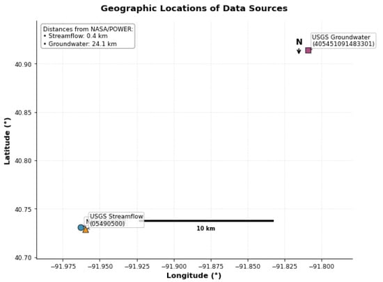
Figure 1.
Geographic locations of the data sources used in the study: NASA/POWER grid point, USGS streamflow gauge at Keosauqua (Site 05490500), and USGS groundwater well in Jefferson County (Site 405451091483301).
3.2. The Kolmogorov–Zurbenko (KZ) Filter
The Kolmogorov–Zurbenko (KZ) filter is a smoothing technique used to decompose time series data into distinct components. It separates short-term noise from longer-term patterns, highlighting underlying trends by repeatedly applying a simple moving average. The filter is defined by two main parameters: the window size, m, which determines the number of neighboring points included in the average, and the number of iterations, k, which specifies how many times the averaging is applied. By adjusting these parameters, one can reduce the influence of short-term fluctuations while isolating specific components of interest, such as seasonal cycles or long-term trends. This capability is instrumental in environmental time series, where multiple sources of variation often overlap, making it crucial for accurate analysis.
Formally, a time series is smoothed by applying a moving average of width m for k iterations:
where denotes the moving average operator with window size m. Figure 2 shows the decomposition of the T2M time series using the KZ filter with a window size of and iterations. The choice of m captures the full annual cycle in daily data, while provides sufficient smoothing without overfitting short-term fluctuations. This configuration removes seasonal cycles and transient variations, facilitating the identification of key long-term temperature patterns.
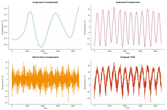
Figure 2.
KZ decomposition of the T2M time series using parameters and , separating the data into long-term, seasonal, and short-term components.
In Figure 2, the top-left plot shows the long-term trend, which smooths short-term fluctuations to highlight slow climatic changes. The top-right plot displays the seasonal component, representing the recurring annual cycle, with regular summer and winter peaks and troughs. The bottom-left plot illustrates the short-term component, capturing high-frequency variations and noise, likely due to weather disturbances or local variability. Finally, the bottom-right plot presents the original T2M time series, where long-term patterns are more complex to discern due to the combination of seasonal and short-term variations.
By separating the time series into these components, the KZ filter provides a clearer understanding of temperature dynamics across multiple time scales.
Through the application of this filter, time series data undergoes decomposition as follows:
In this context, denotes the raw (original) time series, denotes the long-term component, denotes the seasonal-term component, and denotes the short-term component.
3.3. Multicollinearity in Decomposed Feature Spaces
While temporal decomposition enhances feature representation by isolating scale-specific patterns, it can introduce multicollinearity. Decomposing multiple predictor variables using the same filter parameters generates components (long-term, seasonal, and short-term) that often exhibit strong correlations within each timescale. For example, the long-term components of different climate variables may share trends driven by overarching climate modes, while seasonal components reflect synchronized annual cycles.
This issue has been observed in other decomposition-based forecasting frameworks. For instance, multivariate variational mode decomposition (MVMD) applied to river water level forecasting revealed that intrinsic mode functions (IMFs) from different hydrological variables exhibit substantial collinearity, requiring additional feature selection to reduce redundancy [31]. Similarly, studies addressing the “curse of dimensionality and multicollinearity” in decomposition-based models have employed specialized regularization techniques to stabilize predictions [32]. Across hybrid models combining signal decomposition with machine learning, correlated components can destabilize linear models and complicate interpretability [33].
In our framework, although the KZ filter effectively isolates physically meaningful components, the resulting feature space still contains inherent correlations. This explains why Ridge and Lasso regression—with their built-in collinearity mitigation—performed exceptionally well in the decomposed feature space, often rivaling more complex tree-based ensembles.
Table 3 summarizes the most significant correlations among the meteorological and hydrological variables. Several strong relationships are evident, particularly between precipitation (PRECTOTCORR) and soil moisture (GWETROOT) in the long-term component (), reflecting their close hydrological coupling. Relative humidity (RH2M) also shows high positive correlations with both soil moisture () and precipitation (), indicating consistent moisture interactions within the system. Temperature (T2M) exhibits strong positive correlations with solar radiation across both seasonal and long-term components, while its negative correlation with wind speed () reflects typical thermodynamic dynamics. Notably, groundwater levels are inversely correlated with soil moisture (), highlighting the subsurface recharge–discharge relationships. Overall, these high correlations underscore the interconnected nature of surface–atmosphere processes in the study region.
Table 3.
High correlation pairs shown in the heatmap.
Figure 3 visually represents these relationships through a correlation heatmap, where darker shades indicate stronger positive or negative associations among the variables.
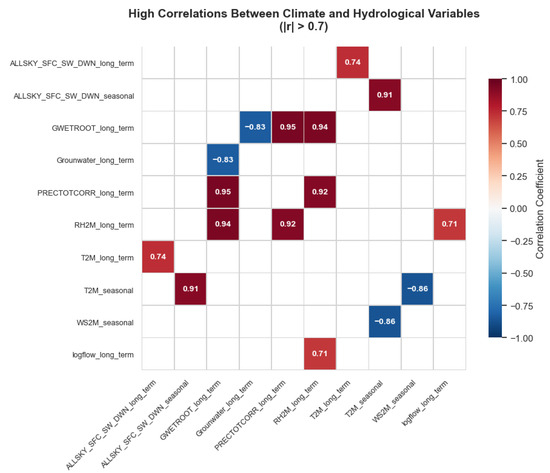
Figure 3.
High correlations between climate and hydrological variables.
4. Results
This section presents a comprehensive analysis of model performance across different temporal scales, starting with the raw data as a baseline and progressing to component-specific and integrated modeling approaches.
4.1. Analysis of Raw Data
All variables were standardized to have a mean of zero and a standard deviation of one, ensuring comparability across different scales. We first applied a multiple linear regression model, allowing the influence of each independent variable on the dependent variable to be quantified through the regression coefficients, as shown in Equation (2).
This interpretable and straightforward framework allows for the assessment of each predictor’s contribution; however, it may be too restrictive for complex real-world data. To address this, we extend the analysis using advanced methods. Ridge and Lasso regression enhance linear models by mitigating multicollinearity and selecting the most critical variables. Random Forest captures nonlinear relationships and interactions through an ensemble of decision trees. At the same time, XGBoost builds sequential trees to reduce errors and uncover subtle patterns, making it particularly effective for modeling the behavior of raw data. Model performance was evaluated using walk-forward validation, which trains on past observations and tests on future data to simulate real-world forecasting. The results (Figure 4) indicate that Random Forest and XGBoost outperform the linear models, achieving lower errors and higher predictive accuracy.
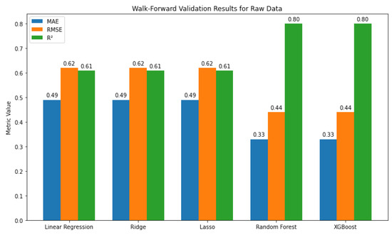
Figure 4.
Walk-forward validation results for raw data.
Moreover, as shown in Figure 5, solar radiation (ALLSKY_SFC_SW_DWN) consistently emerged as the most influential predictor across all models, while GWETROOT exhibited the most substantial adverse effect. Precipitation (PRECTOTCORR) and soil moisture gained higher importance in XGBoost, suggesting potential nonlinear effects, whereas WS2M consistently had minimal influence.
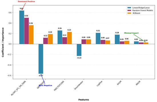
Figure 5.
Feature (Predictor) importance across models, highlighting solar radiation as dominant, GWETROOT as most negative, and the minimal impact of WS2M.
Figure 6 compares the actual time series with predictions from five models: Linear, Ridge, Lasso, Random Forest, and XGBoost. The linear, Ridge, and Lasso models each achieved a correlation coefficient of 0.78, capturing the general pattern but struggling to capture finer fluctuations. In contrast, Random Forest and XGBoost performed better, each reaching a correlation of nearly 0.90, closely following the actual values, particularly around peaks and troughs. These results suggest that ensemble methods are better suited for capturing complex or highly variable patterns in the data.
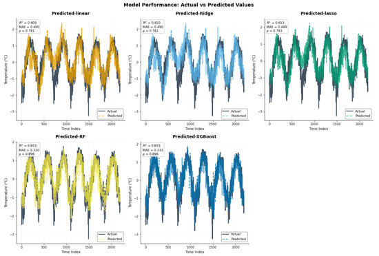
Figure 6.
Time series of actual values versus model predictions with Pearson correlation coefficients () for the raw data.
4.2. Long-Term Component Analysis
This section focuses on the long-term component of the target variable, analyzed using regression and ensemble models to capture underlying trends over time. Equation (3) presents the mathematical formulation of the linear regression model for the long-term component.
The long-term equation above uses the same notation as the raw data equation, with terms applied exclusively to the long-term component.
As can be seen in Figure 7, Tree-based models (RF, XGBoost) outperformed linear ones, achieving the lowest errors and highest R2 (0.91).
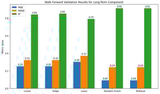
Figure 7.
Walk-forward validation results for long-term data.
Figure 8 shows ALLSKY_SFC_SW_DWN and GWETROOT as the strongest long-term drivers, while PRECTOTCORR and RH2M exert negative effects; tree-based models reduce coefficient magnitudes but confirm solar radiation as dominant and highlight RH2M’s nonlinear role.
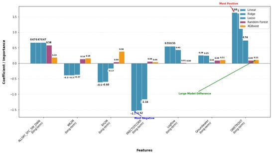
Figure 8.
Bar chart of long-term feature contributions across models, indicating ALLSKY_SFC_SW_DWN and GWETROOT as the strongest positive drivers, while PRECTOTCORR and RH2M show negative effects.
Figure 9 compares the actual long-term values with predictions from five models. Random Forest and XGBoost provide the closest match to the observed data, each achieving a correlation of 0.96, with their curves closely aligned across the time range. Linear and Ridge models also track the overall pattern well, each reaching a correlation of 0.94. Lasso performs slightly worse, with more noticeable deviations around turning points, at 0.93. Nevertheless, all models capture the main shape of the data, indicating reasonable predictive performance.
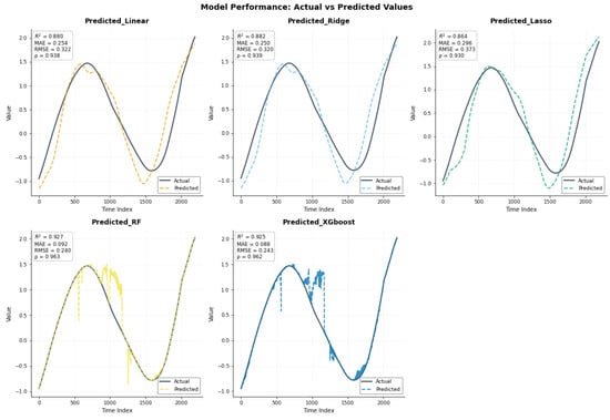
Figure 9.
Time series of actual values versus model predictions with Pearson correlation coefficients () for the long-term.
4.3. Seasonal-Term Component Analysis
This section focuses on evaluating model performance in capturing the seasonal variation of the target variable. Equation (4) presents the mathematical formulation of the linear regression model for the seasonal component.
The seasonal-term equation uses the same notation as the raw data equation, with all terms applied specifically to the seasonal component.
Figure 10 presents walk-forward cross-validation results for T2M_seasonal_term. Linear and Ridge models perform similarly ( 0.14, , ), while Lasso performs slightly worse. Random Forest and XGBoost achieve the lowest errors and , closely tracking the observed seasonal patterns.
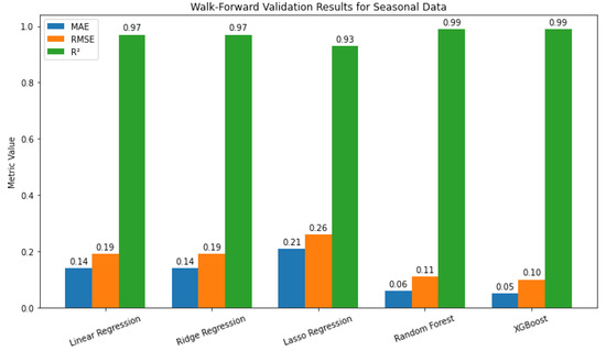
Figure 10.
Walk-forward validation results for seasonal data.
As shown in Figure 11, in the linear models, ALLSKY_SFC_SW_DWN_seasonal exhibits the most potent positive effect, WS2M_seasonal is moderately negative, and other predictors have a minor influence. In Random Forest and XGBoost, ALLSKY_SFC_SW_DWN_seasonal remains the most important predictor, WS2M_seasonal becomes positive, and the remaining variables contribute little, indicating that seasonal variation is primarily driven by solar radiation and wind speed.
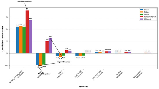
Figure 11.
Walk-forward cross-validation results for T2M_seasonal_term.
Figure 12 compares the actual seasonal values with predictions from five models. The linear models (Linear, Ridge, Lasso) show strong alignment with the observed data (), whereas Random Forest and XGBoost achieve nearly perfect fits (). The combined plot confirms that the tree-based models track the seasonal pattern most accurately, while the linear models still perform well, exhibiting only slight deviations.
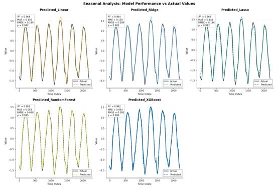
Figure 12.
Time series of actual values versus model predictions with Pearson correlation coefficients () for seasonal variations.
4.4. Short-Term Component Analysis
Given the relatively weaker performance of conventional models on short-term components, this section is divided into two parts: the first applies the same models used for the long-term and seasonal components, while the second explores alternative modeling strategies aimed at improving predictive accuracy.
4.4.1. Baseline Modeling Using Regression and ML
In this subsection, we apply the same set of standard regression and machine learning models previously used for the long-term and seasonal components to the short-term data, establishing a baseline for comparison. Equation (5) presents the mathematical formulation of the linear regression model for the short-term component.
The short-term equation above uses the same notation as the raw data equation, with terms applied exclusively to the short-term component.
Figure 13 shows that all models performed similarly on the short-term component. The linear models exhibited identical MAE (0.69) and (0.21), with Lasso showing a slightly higher RMSE. Random Forest achieved the best performance, with the lowest errors and highest (0.23), while XGBoost performed the worst, with the highest errors and lowest (0.19). Overall, Random Forest provided only a modest improvement over the linear models.
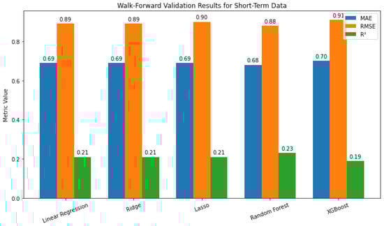
Figure 13.
Walk-forward validation results for short-term data.
Linear models generally assign positive coefficients to most predictors (Figure 14), with RH2M_short_term exhibiting the strongest effect (≈0.50). In contrast, tree-based models assign lower importance to this variable while highlighting nonlinear roles for Groundwater and GWETROOT, which have negative linear coefficients but positive importance in Random Forest and XGBoost. Overall, most predictors contribute modestly and consistently across models, with notable differences in how linear and tree-based methods capture their effects.
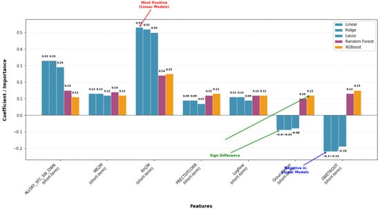
Figure 14.
Walk-forward cross-validation results for T2M short-term.
Figure 15 illustrates how the models capture the short-term component of the data. The linear models (Linear, Ridge, and Lasso) exhibit similar performance, each achieving a correlation of approximately 0.46 with the actual values, indicating only a modest ability to explain short-term fluctuations. Random Forest shows a slightly higher correlation of 0.48, but the improvement is minimal, while XGBoost performs similarly to the linear models. Overall, the combined plot demonstrates that none of the models fully capture the irregular short-term variations, as all predictions remain close to the mean relative to the more volatile actual series. These results suggest that short-term dynamics are more challenging to model with these methods and may require more advanced approaches or additional features.
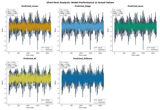
Figure 15.
Time series of actual values versus model predictions for the short term.
4.4.2. Modeling Using Specialized Techniques
To improve upon the baseline results, this subsection explores a range of specialized modeling techniques designed to better capture the dynamics of short-term components, with the goal of enhancing predictive accuracy.
The short-term component captures high-frequency, irregular fluctuations, which are more volatile and less predictable than trend or seasonal patterns [34,35,36]. Figure 16 shows that the Univariate LSTM and AutoReg models performed best (), with low errors, effectively capturing short-term dependencies. Moderate performance was observed for the Ensemble Voting Regressor and Exponential Smoothing (), while SVR and PLS Regression exhibited limited predictive power. Harmonic Regression performed poorly (), and the Multivariate LSTM underperformed (), suggesting overfitting or difficulty in handling multivariate inputs. Default Python 3.10 (64 bit) settings were used for consistency, although further hyperparameter tuning could improve performance. These results indicate that the external explanatory variables in the multivariate models may have limited relevance for short-term fluctuations, which appear to be better captured through temporal dependencies within the target variable itself.
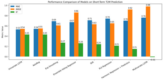
Figure 16.
Performance evaluation of specialized models for short-term data.
4.5. Additive Model Analysis
In this section, we present an additive framework for representing the surface air temperature series by integrating its short-term variations, seasonal pattern, and long-term trend. Equation (6) provides the mathematical formulation for linear regression; a similar approach can be applied to Ridge and Lasso regression, with their respective regularization constraints taken into account. Unlike Ridge and Lasso, which extend linear regression through explicit regularization terms, Random Forest and XGBoost do not rely on a single analytical equation. Instead, they generate predictions through ensembles of decision trees, governed by algorithmic rules and hyperparameter settings.
Here, represents the raw dependent variable; are the long-term component variables with corresponding coefficients ; represent the seasonal-term component with coefficients ; and represent the short-term component variables with coefficients . The term denotes the error at time t.
Tree-based ensembles clearly outperform linear methods. XGBoost shows the best performance (MAE = 0.22, RMSE = 0.29, ), closely followed by Random Forest (MAE = 0.23, RMSE = 0.30, ) (Figure 17), highlighting the effectiveness of ensemble models in capturing complex nonlinear relationships. Among linear models, Ridge Regression performs best, slightly outperforming Lasso and matching the accuracy of Linear Regression, while Random Forest and XGBoost achieve the highest overall accuracy. In summary, tree-based ensembles excel at modeling complex, nonlinear dependencies, whereas Ridge offers a more straightforward and more interpretable alternative.
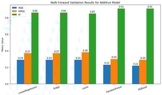
Figure 17.
Walk-forward validation results for additive model.
The feature importance analysis (Figure 18) provides key insights into how different predictors contribute to model performance across temporal scales, physical categories, and learning algorithms. At the individual-feature level (top-left panel), solar radiation-related variables, particularly the seasonal component of ALLSKY_SFCS_DWN, consistently emerge as the most influential across all models. This dominance reflects the primary role of radiative forcing in driving temperature variability, especially at seasonal frequencies. Wind speed and groundwater-related predictors also show moderate contributions, whereas short-term flow-related variables display relatively minor influence.
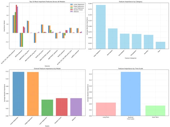
Figure 18.
Walk-forward cross-validation results for additive model.
When aggregated by physical category (top-right panel), solar radiation exhibits the highest mean importance, followed by wind speed and groundwater indices, reaffirming their strong explanatory power in the additive framework. Precipitation and humidity yield lower contributions, suggesting that their effects on temperature may be more indirect or scale-dependent.
The bottom-left panel compares overall feature importance across model families. Ridge and Linear Regression demonstrate the highest average importance, indicating a strong reliance on key predictors and suggesting that regularization enhances the interpretive stability of linear models. Tree-based models (Random Forest and XGBoost), while effective in performance, distribute importance more diffusely due to their ability to model interactions and nonlinearities.
Finally, the time-scale analysis (bottom-right panel) reveals that seasonal components contribute substantially more than long-term and short-term features, highlighting the comparatively high predictability and signal strength at seasonal scales. Long-term predictors retain a moderate influence, likely reflecting broad climatic trends, whereas short-term components show the lowest importance, consistent with their lower predictability and higher stochasticity observed in model evaluation.
Overall, these findings validate the decomposition-based approach by demonstrating that model learning is strongly weighted toward physically interpretable seasonal drivers and that regularized linear models effectively capture dominant relationships while retaining parsimony.
Figure 19 summarizes the numerical results, illustrating how each component contributes to the model’s output across different methods. In the top row, the three linear models—Linear Regression, Ridge, and Lasso—exhibit very similar behaviors, each achieving a correlation coefficient of 0.93 with the observed values. All three models capture the overall wave-like pattern of the data well, but tend to miss sharper turning points, particularly during steep rises and drops, where predictions either lag slightly or fail to reach the full peaks and troughs of the actual series.
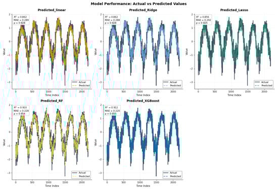
Figure 19.
Time series of actual values versus model predictions for additive models.
In the lower row, Random Forest and XGBoost provide a noticeably closer fit to the observed data, with correlation coefficients of 0.95 and 0.96, respectively. Their prediction lines nearly overlap the actual series throughout the entire period. XGBoost, in particular, captures the full amplitude and direction of variation, even at the extremes, demonstrating a superior ability to learn the underlying structure, especially in regions where the signal exhibits rapid shifts or nonlinear changes.
5. Residuals and Prediction Analysis
This section provides a comprehensive diagnostic evaluation of model residuals for all methods, along with an analysis of prediction uncertainty specifically for linear models. Detailed assessments are presented for Models 2 and 6. A comprehensive residual analysis and prediction interval analysis were performed to evaluate key statistical assumptions and to quantify and compare the predictive uncertainty for Models 2 and 6. Graphical diagnostics illustrate the residual patterns using a linear regression model as a representative case. The results for the residual and prediction interval analyses of Model 2 are presented in Table 4 and Table 5. The same analyses were performed for Model 6, and the corresponding results are shown in Table 6 and Table 7.
Table 4.
Comparative diagnostics of different regression and machine learning models for the raw data.
Table 5.
Coverage, average confidence interval width, and practical uncertainty for model 2.
Table 6.
Comparative diagnostics of different regression and machine learning models for the decomposed data.
Table 7.
Coverage, average confidence interval (CI) width, and practical uncertainty for model 6.
While this study provides comprehensive uncertainty quantification for linear models, the computational demands of our walk-forward validation scheme made extensive uncertainty analysis for machine learning models prohibitive. Methods such as conformal prediction or Bayesian deep learning would require substantial additional computation time. Future work could focus on developing efficient uncertainty quantification methods designed explicitly for component-wise forecasting frameworks with complex machine learning models.
5.1. Residual Diagnostics and Prediction Analysis for Model 2 (Raw Data)
This subsection presents the residual analysis and confidence interval evaluation for Model 2, assessing both statistical assumptions and prediction uncertainty calibration.
5.1.1. Residual Diagnostics for Model 2
The residual diagnostics presented in Figure 20a–d provide insights into the adequacy of the linear regression model. Panel (a) shows the residuals versus fitted values, where the residuals are centered around zero, indicating that the model is generally unbiased. However, the uneven spread of points suggests the presence of heteroscedasticity, implying non-constant variance across fitted values. Panel (b) displays the histogram of residuals, which approximately follows a bell-shaped distribution, supporting the assumption of normality, although slight deviations from perfect symmetry can be observed. Panel (c), the Q–Q plot, further confirms this pattern, as the residual points closely follow the reference line, indicating that the residuals are approximately normally distributed, with minor deviations at the tails. Finally, panel (d) plots the residuals over index/time, revealing noticeable patterns and clustering around zero, which indicates the presence of autocorrelation and suggests that the residuals are not entirely independent.
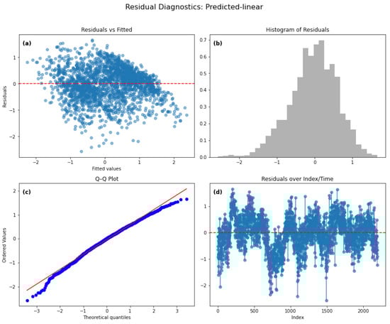
Figure 20.
Residual diagnostics for the Linear Regression model for the Raw Data. Diagnostic plots for the regression model: (a) Residuals versus fitted values; (b) Histogram of residuals; (c) Q–Q plot showing approximate normality; (d) Residuals versus index/time.
Table 4 presents the diagnostic statistics for all tested models for the raw data. The Residual Mean indicates that the Random Forest and XGBoost models achieved the smallest average residuals, suggesting superior predictive accuracy compared to the Linear, Ridge, and Lasso models. The Durbin–Watson statistic values below 2 for the linear-based models indicate positive autocorrelation in residuals, whereas values closer to 2 for Random Forest and slightly above 1 for XGBoost suggest reduced autocorrelation. The Breusch–Pagan LM test p-values are extremely small across all models, indicating significant heteroscedasticity in residuals. Similarly, the Shapiro–Wilk test p-values are far below the typical significance threshold, implying that residuals deviate from normality for all models. Overall, while Random Forest and XGBoost demonstrate lower residuals and improved autocorrelation behavior, none of the models fully satisfy the assumptions of homoscedasticity and normality. As can be seen, traditional residual diagnostics are reported for all models, enabling direct comparison. It should be noted that while violations of normality, independence, and homoscedasticity compromise the statistical inference capabilities of linear models, machine learning methods are primarily evaluated on predictive accuracy. These diagnostics nonetheless reveal systematic patterns in model errors across different approaches.
5.1.2. Prediction Interval and Uncertainty Analysis for Model 2
The model comparison metrics in Table 5 indicate that all three models—Linear Regression, Ridge, and Lasso—demonstrate similar predictive performance in terms of uncertainty quantification. The coverage values are consistently around 0.93, suggesting that approximately 93% of the actual observations fall within the estimated prediction intervals. This indicates that the models provide reliable probabilistic forecasts, which are slightly conservative compared to the standard 95% nominal confidence level commonly used in predictive modeling. The average confidence interval (CI) width ranges from 2.25 to 2.26, representing the typical span within which predictions are expected to fall at the stated confidence level. This relatively narrow range indicates that the models yield precise estimates with moderate uncertainty. The practical uncertainty, defined as the ratio of the average CI width to the standard deviation of the target variable, remains consistently at 1.13. This suggests that predictive uncertainty slightly exceeds the inherent variability of the data, reflecting a moderate yet stable level of predictive precision across models.
5.2. Residual Diagnostics and Prediction Analysis for Model 6 (Decomposed Data)
The residual diagnostics and confidence interval evaluation for Model 6 are examined.
5.2.1. Residual Diagnostics for Model 6
The residual diagnostics for the combined model constructed using decomposed data are presented in Figure 21a–d. Panel (a) displays the residuals versus fitted values, where the residuals are well-centered around zero with no clear systematic pattern, indicating that the model is generally unbiased and the variance appears more homogeneous compared to the linear model. Panel (b) shows the histogram of residuals, which closely resembles a normal distribution, supporting the assumption of normality with minimal skewness. Panel (c), the Q–Q plot, further reinforces this observation as the residual points closely follow the reference line across most quantiles, with only slight deviations at the extreme tails, indicating that the residuals are approximately normally distributed. Finally, panel (d) illustrates the residuals over index/time, showing that the residuals fluctuate randomly around zero without distinct patterns or strong clustering, suggesting a reduction in autocorrelation compared to the non-decomposed model. Overall, these diagnostics indicate that the combined model provides a better fit, with improved adherence to the assumptions of linear regression.
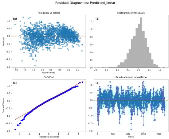
Figure 21.
Residual diagnostics for the linear regression model for the decomposed data. Diagnostic plots for the regression model: (a) Residuals versus fitted values; (b) Histogram of residuals; (c) Q–Q plot showing approximate normality; (d) Residuals versus index/time.
Table 6 presents the diagnostic statistics for all tested models for the decomposed data. The Residual Mean indicates that the Random Forest and XGBoost models achieved the smallest average residuals, suggesting superior predictive accuracy compared to the linear, Ridge, and Lasso models. The Durbin–Watson statistic values below 2 for the linear-based models indicate positive autocorrelation in residuals, whereas values closer to 2 for Random Forest and slightly above 1 for XGBoost suggest reduced autocorrelation. The Breusch–Pagan LM test p-values are extremely small across all models, indicating significant heteroscedasticity in residuals. Similarly, the Shapiro–Wilk test p-values are far below the typical significance threshold, implying that residuals deviate from normality for all models. Overall, while Random Forest and XGBoost demonstrate lower residuals and improved autocorrelation behavior, none of the models fully satisfy the assumptions of homoscedasticity and normality.
5.2.2. Prediction Interval and Uncertainty Analysis for Model 6
To complement the residual diagnostics, a prediction interval and uncertainty analysis were conducted for the linear methods. Table 7 reports the empirical coverage, average confidence interval (CI) width, and practical uncertainty. All three linear models achieved coverage rates close to the nominal 95% level, indicating well-calibrated prediction intervals. Ridge regression exhibited the highest coverage (0.9498) with an interval width comparable to Linear Regression, while Lasso produced slightly wider intervals and marginally lower coverage. These results suggest that the predictive uncertainty of the linear methods is relatively narrow and consistent, with Ridge offering the most favorable balance between calibration and interval sharpness. This analysis is presented here for linear models to illustrate the procedure; in future work, similar uncertainty evaluations will be extended to machine learning methods for a more comprehensive comparison.
6. Discussion and Conclusions
The walk-forward validation results across the three temporal components—long-term, seasonal, and short-term—reveal fundamental differences in model behavior and predictive skill, providing new insights into the structure of temperature variability. These findings highlight the central contribution of this study: the development and benchmarking of a dual forecasting architecture that combines component-wise and additive multi-scale modeling within a unified KZ-decomposition framework. By systematically evaluating both independent component models and a unified additive model, we demonstrate how temporal decomposition can expose scale-dependent predictability while simultaneously enhancing overall forecasting accuracy.
By decomposing the original series using the Kolmogorov–Zurbenko (KZ) filter and modeling each component independently, our approach isolates scale-specific dynamics that are typically obscured when modeling the raw signal. A comparative analysis across components confirms that optimal forecasting strategies vary by temporal scale, thereby validating the rationale for decomposition-based modeling. The unified additive model, which integrates all decomposed predictors to forecast the original T2M, further demonstrates that learning directly from multi-scale features enables the discovery of interactions across temporal domains—a key advantage over strictly separate component modeling.
6.1. Performance Across Temporal Components
For the long-term component, tree-based ensemble models (Random Forest and XGBoost) achieved the highest accuracy (), indicating their practical ability to capture complex, nonlinear patterns. Ridge regression, however, delivered highly competitive results, substantially outperforming ordinary linear regression. This underscores the effectiveness of regularization in handling multicollinearity inherent in decomposed environmental predictors—a novel and practically relevant finding.
The seasonal component exhibited the strongest predictability across all algorithms. Tree-based ensembles achieved near-perfect accuracy (), while Linear and Ridge regression also performed exceptionally well (). These results confirm that seasonal temperature variability is dominated by stable, quasi-linear relationships with its predictors, indicating that regularized linear models can serve as both accurate and interpretable alternatives to complex ensembles for seasonal forecasting within the KZ framework.
In contrast, the short-term component remained challenging for all models (), suggesting that this scale is strongly influenced by stochastic atmospheric processes or unresolved local variability. Specialized time-series models, such as univariate LSTM and AutoReg, yielded moderate improvements (), suggesting that high-frequency dynamics may necessitate explicitly temporal architectures rather than regression-based approaches.
6.2. Framework Comparison and Model Insights
The comparison between the raw (non-decomposed) and the component-wise additive unified frameworks demonstrates that temporal decomposition fundamentally enhances both model performance and interpretability. Modeling the original series directly forced algorithms to approximate multiple physical processes operating on different time scales within a single functional relationship, limiting accuracy and generalizability. In contrast, the component-wise additive framework—where each predictor was first decomposed into long-term, seasonal, and short-term components before unified model training—enabled models to learn scale-specific relationships while maintaining a single, interpretable prediction structure.
Across all model classes, the additive KZ-based framework yielded substantial improvements. Ridge regression benefited most, with increasing from 0.61 (raw) to 0.86 (additive) and MAE decreasing from 0.49 to 0.29. This confirms that combining regularization with decomposition effectively mitigates multicollinearity and enhances stability. Lasso regression exhibited similar trends, highlighting the robustness of regularized linear models in decomposed feature spaces. Tree-based ensembles, particularly XGBoost, also achieved higher accuracy within the additive framework ( up to 0.91), demonstrating that even nonlinear learners benefit from structured decomposition.
Residual and uncertainty analyses further supported these gains: models trained on additive decomposed features exhibited narrower confidence intervals and improved coverage, indicating more accurate and better-calibrated predictions. The unified additive approach thus preserves physical interpretability—each feature corresponds to a known temporal process—while delivering accuracy comparable to, or exceeding, more complex nonlinear alternatives.
6.3. Limitations and Future Research
This study is limited to a single geographic location and time span, and the short-term component remains challenging to predict. Future research should extend the framework to multiple locations and investigate more specialized models for capturing short-term dynamics. The promising performance of regularized linear models, particularly Ridge regression, suggests their inclusion as benchmark methods in future multi-scale forecasting studies, offering a practical compromise between complex ensembles and simple linear models.
Author Contributions
Conceptualization, D.Z.; Methodology, K.A.-S. and D.Z.; Software, K.A.-S. and A.M.; Validation, K.A.-S.; Formal analysis, K.A.-S., D.Z. and A.M.; Investigation, K.A.-S., D.Z. and K.T.; Resources, K.A.-S. and K.T.; Data curation, K.A.-S.; Writing—original draft, K.A.-S.; Writing—review and editing, A.F.; Visualization, A.F.; Supervision, A.F., K.T. and A.M.; Project administration, A.F. and A.M. All authors have read and agreed to the published version of the manuscript.
Funding
This research received no external funding.
Data Availability Statement
The data presented in this study are openly available in NASA/POWER [POWER Project] [https://power.larc.nasa.gov/data-access-viewer/ 6 March 2025)] [nasa 2024].
Acknowledgments
The authors would like to acknowledge the anonymous reviewers for their careful reading of the manuscript.
Conflicts of Interest
The authors declare no conflicts of interest.
References
- Wu, L.X.; An, J.L.; Jin, D. Predictive Model for O3 in Shanghai Based on the KZ Filtering Technique and LSTM. Huan Jing Ke Xue 2024, 45, 5729–5739. [Google Scholar] [CrossRef]
- Nafarrate, A.; Petisco-Ferrero, S.; Idoeta, R.; Herranz, M.; Sáenz, J.; Ulazia, A.; Ibarra-Berastegui, G. Applying the Kolmogorov–Zurbenko Filter Followed by Random Forest Models to 7Be Observations in Spain (2006–2021). Heliyon 2024, 10, e30820. [Google Scholar] [CrossRef]
- Kumar, V.; Sur, S.; Senarathna, D.; Gurajala, S.; Dhaniyala, S.; Mondal, S. Quantifying Impact of Correlated Predictors on Low-Cost Sensor PM2.5 Data Using KZ Filter. Front. Appl. Math. Stat. 2024, 10, 1368147. [Google Scholar] [CrossRef]
- Ajuji, M.; Dawaki, M.; Mohammed, A.; Ahmad, A. Estimating Residential Natural Gas Demand and Consumption: A Hybrid Ensemble Machine Learning Approach. Vokasi Unesa Bull. Eng. Technol. Appl. Sci. 2025, 2, 549–557. [Google Scholar] [CrossRef]
- Andrianarisoa, S.H.; Ravelonjara, H.M.; Suddul, G.; Foogooa, R.; Armoogum, S.; Sookarah, D. A Deep Learning Approach to Fake News Classification Using LSTM. Vokasi Unesa Bull. Eng. Technol. Appl. Sci. 2025, 2, 593–601. [Google Scholar] [CrossRef]
- Yang, W.; Zurbenko, I. Kolmogorov–Zurbenko Filters. Wiley Interdiscip. Rev. Comput. Stat. 2010, 2, 340–351. [Google Scholar] [CrossRef]
- Zurbenko, I.G.; Cyr, D.D. Climate Fluctuations in Time and Space. Clim. Res. 2011, 46, 67–76. [Google Scholar] [CrossRef][Green Version]
- Zurbenko, I.G.; Luo, M. Restoration of Time-Spatial Scales in Global Temperature Data. Am. J. Clim. Change 2012, 1, 154–163. [Google Scholar] [CrossRef][Green Version]
- Zurbenko, I.G.; Smith, D. Kolmogorov–Zurbenko Filters in Spatiotemporal Analysis. Wiley Interdiscip. Rev. Comput. Stat. 2018, 10, e1419. [Google Scholar] [CrossRef]
- Agbehadji, I.E.; Obagbuwa, I.C. Systematic Review of Machine Learning and Deep Learning Techniques for Spatiotemporal Air Quality Prediction. Atmosphere 2024, 15, 1352. [Google Scholar] [CrossRef]
- Yao, T.; Ye, H.; Wang, Y.; Zhang, J.; Guo, J.; Li, J. Kolmogorov–Zurbenko Filter Coupled with Machine Learning to Reveal Multiple Drivers of Surface Ozone Pollution in China from 2015 to 2022. Sci. Total Environ. 2024, 949, 175093. [Google Scholar] [CrossRef]
- Mahmood, K.K. Statistical Analysis for Decomposed Multivariate Time Series Data with an Application to Water Discharge Forecasting. Ph.D. Thesis, University of Brighton, Brighton, UK, 2019. [Google Scholar]
- Kişmiroğlu, C.; Isik, O. Temperature Prediction Using Transformer–LSTM Deep Learning Models and SARIMAX from a Signal Processing Perspective. Appl. Sci. 2025, 15, 9372. [Google Scholar] [CrossRef]
- Chen, Q.; Cai, C.; Chen, Y.; Zhou, X.; Zhang, D.; Peng, Y. TemproNet: A Transformer-Based Deep Learning Model for Seawater Temperature Prediction. Ocean Eng. 2024, 293, 116651. [Google Scholar] [CrossRef]
- Huang, X.; Zhuang, X.; Tian, F.; Niu, Z.; Chen, Y.; Zhou, Q.; Yuan, C. A Hybrid ARIMA–LSTM–XGBoost Model with Linear Regression Stacking for Transformer Oil Temperature Prediction. Energies 2025, 18, 1432. [Google Scholar] [CrossRef]
- Çınarer, G. Hybrid Deep Learning and Stacking Ensemble Model for Time Series-Based Global Temperature Forecasting. Electronics 2025, 14, 3213. [Google Scholar] [CrossRef]
- Luo, Z.; Hou, C.; Wang, H. Research on Temperature Prediction Model Based on DNN–LSTM and Multi-Head Attention. In Proceedings of the 2025 5th International Symposium on Computer Technology and Information Science (ISCTIS), Xi’an, China, 16–18 May 2025; pp. 88–91. [Google Scholar] [CrossRef]
- Cao, Y.; Zhai, J.; Zhang, W.; Zhou, X.; Zhang, F. MTTF: A Multimodal Transformer for Temperature Forecasting. Int. J. Comput. Appl. 2024, 46, 122–135. [Google Scholar] [CrossRef]
- Krivoguz, D.; Ioshpa, A.; Chernyi, S.; Zhilenkov, A.; Kustov, A.; Zinchenko, A.; Podelenyuk, P.; Tsareva, P. Enhancing long-term air temperature forecasting with deep learning architectures. J. Robot. Control 2024, 5, 706–716. [Google Scholar] [CrossRef]
- Wang, H. Weather Temperature Prediction Based on LSTM and Transformer. SPIE Conf. Proc. 2024, 13445, 134450R. [Google Scholar] [CrossRef]
- Tarunkumar, K.; Umesh, A.; Humbarwadi, M.; Sohan, B.; Bhargavi, M.S. Exploring the Efficacy of Deep Learning and Statistical Approaches in Temperature Forecasting. In Proceedings of the 2024 International Conference on Emerging Technologies and Innovation for Sustainability (EmergIN), Greater Noida, India, 20–21 December 2024. [Google Scholar] [CrossRef]
- Huang, X.; Zhuang, X.; Tian, F.; Niu, Z.; Chen, Y.; Zhou, Q. Transformer Top Oil Temperature Prediction Using Deep Learning Time Series Model. In Proceedings of the 2024 IEEE International Symposium on New Energy and Electrical Technology (ISNEET), Hangzhou, China, 27–29 December 2024. [Google Scholar] [CrossRef]
- Mu, Z.; Chen, Y.; Pan, H.; Jiang, Y. Novel Transformer-Like Predictive Model for Improving the Accuracy of Indoor-Temperature Prediction. Appl. Therm. Eng. 2025, 252, 127120. [Google Scholar] [CrossRef]
- Şevgin, F. Machine Learning-Based Temperature Forecasting for Sustainable Climate Change Adaptation and Mitigation. Sustainability 2025, 17, 1812. [Google Scholar] [CrossRef]
- Zhang, W.; Li, Z.; Tian, Y. Research on Temperature Prediction Based on RF–LSTM Modeling. IEEE TechRxiv 2025. [Google Scholar] [CrossRef]
- Toama, H.J.; Hussein, K.Q. Review of Techniques and Algorithms of Temperature Prediction Using Artificial Intelligence. Iraqi J. Intell. Comput. Inform. (IJICI) 2025, 4, 182–193. [Google Scholar] [CrossRef]
- Mutinda, J.K.; Langat, A.K.; Mwalili, S.M. Forecasting Temperature Time Series Data Using Combined Statistical and Deep Learning Methods: A Case Study of Nairobi County Daily Temperature. Int. J. Math. Math. Sci. 2025, 2025, 4795841. [Google Scholar] [CrossRef]
- Ganesan Kruthika, S.; Rajasekaran, U.; Alagarsamy, M.; Sharma, V. Analysis of Statistical and Deep Learning Techniques for Temperature Forecasting. Recent Adv. Comput. Sci. Commun. 2024, 17, 49–65. [Google Scholar] [CrossRef]
- Liu, S.; Liu, K.; Wang, Z.; Liu, Y.; Bai, B.; Zhao, R. Investigation of a Transformer-Based Hybrid Artificial Neural Networks for Climate Data Prediction and Analysis. Front. Environ. Sci. 2025, 12, 1464241. [Google Scholar] [CrossRef]
- Fu, Y.; Song, J.; Guo, J.; Fu, Y.; Cai, Y. Prediction and Analysis of Sea Surface Temperature Based on LSTM–Transformer Model. Reg. Stud. Mar. Sci. 2024, 78, 103726. [Google Scholar] [CrossRef]
- Ahmadianfar, I.; Farooque, A.A.; Ali, M.; Jamei, M.; Jamei, M.; Yaseen, Z.M. A hybrid framework: Singular value decomposition and kernel ridge regression optimized using mathematical-based fine-tuning for enhancing river water level forecasting. Sci. Rep. 2025, 15, 7596. [Google Scholar] [CrossRef]
- Kordani, M.; Bagheritabar, M.; Ahmadianfar, I.; Samadi-Koucheksaraee, A. Forecasting water quality indices using generalized ridge model, regularized weighted kernel ridge model, and optimized multivariate variational mode decomposition. Sci. Rep. 2025, 15, 16313. [Google Scholar] [CrossRef] [PubMed]
- Jamei, M.; Ali, M.; Malik, A.; Prasad, R.; Abdulla, S.; Yaseen, Z.M. Forecasting daily flood water level using hybrid advanced machine learning based time-varying filtered empirical mode decomposition approach. Water Resour. Manag. 2022, 36, 4637–4676. [Google Scholar] [CrossRef]
- Hyndman, R.J.; Athanasopoulos, G. Forecasting: Principles and Practice; OTexts: Melbourne, Australia, 2018. [Google Scholar]
- Chatfield, C.; Xing, H. The Analysis of Time Series: An Introduction with R; Chapman and Hall/CRC: Boca Raton, FL, USA, 2019. [Google Scholar]
- Shumway, R.H.; Stoffer, D.S. Time Series Analysis and Its Applications: With R Examples; Springer: New York, NY, USA, 2006. [Google Scholar]
Disclaimer/Publisher’s Note: The statements, opinions and data contained in all publications are solely those of the individual author(s) and contributor(s) and not of MDPI and/or the editor(s). MDPI and/or the editor(s) disclaim responsibility for any injury to people or property resulting from any ideas, methods, instructions or products referred to in the content. |
© 2025 by the authors. Licensee MDPI, Basel, Switzerland. This article is an open access article distributed under the terms and conditions of the Creative Commons Attribution (CC BY) license (https://creativecommons.org/licenses/by/4.0/).