Qualitative Analysis of Delay Stochastic Systems with Generalized Memory Effects

Abstract

Fractional stochastic differential equations (FSDEs) are powerful tools for modeling real-world phenomena, as they incorporate both memory effects and stochastic noise. A central focus in their analysis is establishing the well-posedness and regularity of solutions. Moreover, the averaging principle offers a systematic approach to simplify complex dynamical systems by approximating their behavior through time-averaged models. In this paper, we develop a theoretical framework for a class of FSDEs involving the Hilfer–Katugampola derivative. Our main contributions include proving the well-posedness and regularity of solutions, establishing a generalized averaging principle, and demonstrating real-life applications solved via the Euler–Maruyama method. All numerical simulations were conducted using the Python programming language (version 3.11). These results are formulated for the $\tilde{\mathcal{P}}$th moment, providing a unified analysis that extends existing findings.

1. Introduction

The literature includes discussions on various types of fractional operators [1,2,3,4,5]. In recent years, many researchers have adopted the Hilfer–Katugampola fractional derivative (HKFD) in their work, as it serves as an interpolation between several fractional operators, including the Riemann–Liouville (R-L), Caputo, Hadamard, Hilfer, Caputo–Hadamard, Hilfer–Hadamard, Weyl, and Liouville derivatives. The authors in [6] established the existence and uniqueness (Ex-Un) of a fractional model involving the HKFD. In [7], several theoretical results were derived for fractional-order systems involving the HKFD. The study in [8] presented important findings concerning solutions to fractional-order models with the HKFD. The authors of [9] derived solutions for the fractional radial diffusion model with respect to the HKFD. Additionally, in [10], the authors obtained solutions to space-time fractional models using the Mellin transform.

Before introducing the HKFD, we first need to define the Katugampola fractional integral and derivative. The Katugampola fractional integral of order $0<\vartheta <1$ and $\kappa >0$ for the function ℷ is given as follows [11]:

$${}^{\kappa }\mathcal{I}_{{\mathrm{u}}^{\mathrm{+}}}^{\vartheta }\gimel \left(\mathfrak{b}\right)={\displaystyle \frac{{\kappa }^{1-\vartheta }}{\Gamma \left(\vartheta \right)}}{\int }_{\mathrm{u}}^{\mathfrak{b}}{\mathfrak{c}}^{\kappa -1}{\left({\mathfrak{b}}^{\kappa }-{\mathfrak{c}}^{\kappa }\right)}^{\vartheta -1}\gimel \left(\mathfrak{c}\right)\mathrm{d}\mathfrak{c}.$$

(1)

The Katugampola fractional derivative is given as follows [11]:

$$\begin{array}{c}\hfill {}^{\kappa }\mathcal{T}_{{\mathrm{u}}^{\mathrm{+}}}^{\vartheta }\gimel \left(\mathfrak{b}\right)={\displaystyle \frac{{\kappa }^{\vartheta }}{\Gamma (1-\vartheta )}}\left({\mathfrak{b}}^{1-\kappa }{\displaystyle \frac{\mathrm{d}}{\mathrm{d}\mathfrak{b}}}\right){\int }_{\mathrm{u}}^{\mathfrak{b}}{\displaystyle \frac{{\mathfrak{c}}^{\kappa -1}}{{\left({\mathfrak{b}}^{\kappa }-{\mathfrak{c}}^{\kappa }\right)}^{\vartheta }}}\gimel \left(\mathfrak{c}\right)\mathrm{d}\mathfrak{c}.\end{array}$$

The HKFD of order $0<\vartheta <1$ and $0\le \varpi \le 1$ with $\kappa >0$, with respect to $\mathfrak{b}$, is defined as follows [12]:

$$\begin{array}{c}\hfill {}^{\kappa }\mathcal{T}_{{\mathrm{u}}^{\mathrm{+}}}^{\vartheta ,\varpi }\gimel \left(\mathfrak{b}\right)={}^{\kappa }\mathcal{I}_{{\mathrm{u}}^{\mathrm{+}}}^{\varpi (1-\vartheta )}{}^{\kappa }\mathcal{T}_{{\mathrm{u}}^{\mathrm{+}}}^{\lambda }\gimel \left(\mathfrak{b}\right),\lambda =\vartheta +\varpi -\vartheta \varpi .\end{array}$$

(2)

The subsequent fractional derivatives can be interpolated using the HKFD: Caputo–Hadamard ($\varpi =1,\kappa \to 0^{+}$) [13], Caputo-kind ($\varpi =1$) [14], Hilfer–Hadamard ($\kappa \to 0^{+}$) [15], generalized ($\varpi =0$) [16], Hilfer ($\kappa \to 1$) [17], R-L ($\varpi =0,\kappa \to 1$) [18], Hadamard ($\varpi =1,\kappa \to 0^{+}$) [18], Caputo ($\varpi \to 1,\kappa \to 1$) [18], Liouville ($\varpi =0,\kappa \to 1,\mathrm{u}=0$) [18], and Weyl ($\varpi =0,\kappa \to 1,\mathrm{u}=-\infty$) [19].

Implementing HKFD in large-scale systems poses significant computational challenges due to the memory effect, where the current state relies on all previous states. This reliance leads to a considerable increase in computational costs and memory usage as both the system size and simulation time expand. The complicated interactions among subsystems further complicate matters, resulting in more complex equations that are challenging to solve. Additionally, numerical methods for HKFD necessitate small time steps to effectively manage singularities, which exacerbates the computational burden. The nonlocal and high-dimensional characteristics of fractional models also complicate the identification of system parameters and the development of appropriate controllers.

Fractional delay stochastic differential equations (FDSDEs) are mathematical models that incorporate fractional derivatives to account for memory effects, time delays in dynamic interactions, and stochastic processes to represent random or noisy events. These equations are particularly well-suited for systems in which past states, delay effects, and random fluctuations significantly influence the system’s dynamics. FDSDEs find applications in various real-world scenarios, such as finance (e.g., asset pricing with time-lagged market responses) and physics (e.g., viscoelastic materials with delayed stress-strain relationships). By integrating these complex factors, FDSDEs provide a robust framework for analyzing and predicting the behavior of time-dependent and unstable systems.

Numerous scholars have contributed diverse findings to the field of FSDEs. For instance, Kahouli et al. [20] established stability criteria for such systems. Subsequent work has focused on various analytical and practical aspects: the Ex-Un of solutions was confirmed for coupled systems using Picard’s iteration method [21], and controllability was examined for FSDEs with Hilfer fractional derivatives via sectorial operators [22]. Further foundational results in this area were established in [23,24].

Building on this, the authors of [25] proved various qualitative results for FSDEs, while studies concerning specific derivatives, such as the CHFD, have also been explored [26]. Moualkia and Xu [27] extended the analysis to variable-order FSDEs, deriving novel sufficient conditions and obtaining solutions via Picard’s method. Applications of FSDEs are also emerging; for example, a financial chaotic model incorporating an Atangana–Baleanu operator was investigated in [28], complete with numerical solutions and graphical interpretations. Finally, the theory for more complex systems has been advanced by research into Ex-Un for impulsive FSDEs [29] and into the finite-time stability of specific FSDE categories [30].

This research provides substantial new findings for FDSDEs involving the HKFD. The Banach contraction principle (BCP) is utilized to confirm the Ex-Un of solutions. The work further derives the continuous dependence and regularity properties of the solutions to FDSDEs. Interval translation and inequality techniques are employed to validate the averaging principle (Av-Pr).

The validation of our theoretical findings is contingent upon the pivotal application of fundamental inequalities, most notably Jensen’s (Jen-Ineq), the Burkholder–Davis–Gundy (Bu-Da-Gu-Ineq), and Hölder’s (Höl-Ineq). The Bu-Da-Gu-Ineq mostly affects the system’s stochastic part, and it becomes more sensitive as higher moments are used. On the other hand, the Höl-Ineq affects how product terms are separated and can create wider boundaries if the exponents are not set carefully. The Jen-Ineq may also make the bound less strict when expectations are changed between nonlinear terms. Therefore, the overall error bound depends on how these inequalities interact with each other. To obtain more accurate and tighter predictions, one needs to choose the right moment orders and exponents very carefully.

The main contributions of this work are summarized as follows:

• We present a novel analysis of FDSDEs, establishing, for the first time, the existence of unique solutions that depend continuously on initial conditions and the fractional derivative order, alongside the Av-Pr for the HKFD in the $\tilde{\mathcal{P}}$th moment sense.
• Our findings are broadly applicable due to the HKFD’s generality, which incorporates many specific fractional derivatives as special cases.
• A key advancement of our work is the generalization of standard well-posedness and regularity results from the conventional ${\mathrm{L}}^2$ setting to the more comprehensive ${\mathrm{L}}^{\tilde{\mathcal{P}}}$ space.

We consider the following Hilfer–Katugampola FDSDEs:

$$\{\begin{array}{cc}{}^{\kappa }\mathcal{T}_{0^{\mathrm{+}}}^{\vartheta ,\varpi }\gimel \left(\mathfrak{b}\right)=\mathfrak{g}(\mathfrak{b},\gimel \left(\mathfrak{b}\right),\gimel \left(\mathfrak{b}-\varrho \right))+\mathfrak{r}(\mathfrak{b},\gimel \left(\mathfrak{b}\right),\gimel \left(\mathfrak{b}-\varrho \right)){\displaystyle \frac{\mathrm{d}\mathcal{W}\left(\mathfrak{b}\right)}{\mathrm{d}\mathfrak{b}}},\hfill & \\ \gimel \left(0\right)=\nu ,\hfill \end{array}$$

(3)

where ${}^{\kappa }\mathcal{T}_{0^{\mathrm{+}}}^{\vartheta ,\varpi }$ is the HKFD, with its parameters defined by $\vartheta \in \left({\displaystyle \frac{1}{2}},1\right)$, $0<\kappa \le 1$, and $0\le \varpi \le 1$. The term $\varrho \in \mathbb{R}$ represents a constant delay. The functions $\mathfrak{g}:[0,\varsigma ]\times {\mathbb{R}}^{\mathfrak{e}}\times {\mathbb{R}}^{\mathfrak{e}}\to {\mathbb{R}}^{\mathfrak{e}}$ and $\mathfrak{r}:[0,\varsigma ]\times {\mathbb{R}}^{\mathfrak{e}}\times {\mathbb{R}}^{\mathfrak{e}}\to {\mathbb{R}}^{\mathfrak{e}\times \sigma }$ are measurable and continuous. All these elements are defined with respect to a $\sigma$-dimensional Brownian motion $\left({\mathcal{W}}_{\mathfrak{b}}\right)\mathfrak{b}\ge 0$, which itself is defined on a complete filtered probability space $(\Omega ,\mathrm{F},\mathbb{F}={\left({\mathrm{F}}_{\mathfrak{b}}\right)}_{\mathfrak{b}\ge 0},\mathrm{P})$.

The following Section 2 introduces key definitions and outlines the assumptions underpinning the analysis of Hilfer–Katugampola FDSDEs. Section 3.1 establishes the well-posedness of the Hilfer–Katugampola FDSDEs, while Section 3.2 addresses their regularity properties. Section 4 presents results related to Av-Pr. Section 5 illustrates the theoretical findings through two examples. Section 6 summarizes the main conclusions of the study. Finally, we outline directions for future work.

2. Preliminaries

This section presents lemmas, definitions, and assumptions essential for deriving key results.

 Lemma 1 

([31]). Assume that $0<\vartheta <1$, $0\le \varpi \le$1, $\kappa >0$. Then, for a continuously differentiable function $\gimel \left(\mathfrak{b}\right)$, we have the following:

$$\begin{array}{c}\hfill \left({}^{\kappa }\mathcal{I}_{{\mathrm{u}}^{\mathrm{+}}}^{\vartheta }{}^{\kappa }\mathcal{T}_{{\mathrm{u}}^{\mathrm{+}}}^{\vartheta }\gimel \right)\left(\mathfrak{b}\right)=\gimel \left(\mathfrak{b}\right)-{\displaystyle \frac{{}^{\kappa }\mathcal{I}_{{\mathrm{u}}^{\mathrm{+}}}^{1-\vartheta }\gimel \left(0\right)}{\Gamma \left(\vartheta \right)}}{\displaystyle \frac{{({\mathfrak{b}}^{\kappa }-{\mathfrak{c}}^{\kappa })}^{\vartheta -1}}{{\kappa }^{\vartheta -1}}},\end{array}$$

where ${}^{\kappa }\mathcal{I}_{{\mathrm{u}}^{\mathrm{+}}}^{\vartheta }$ and ${}^{\kappa }\mathcal{T}_{{\mathrm{u}}^{\mathrm{+}}}^{\vartheta }$ are the Katugampola fractional integral and derivative, respectively.

 Lemma 2 

([31]). Suppose $0<\vartheta <1$, $0\le \varpi \le 1$, $\kappa >0$, and $\lambda =\vartheta +\varpi -\vartheta \varpi$, then

$$\begin{array}{c}\hfill \left({}^{\kappa }\mathcal{I}_{{\mathrm{u}}^{\mathrm{+}}}^{\lambda }{}^{\kappa }\mathcal{T}_{{\mathrm{u}}^{\mathrm{+}}}^{\lambda }\gimel \right)\left(\mathfrak{b}\right)=\left({}^{\kappa }\mathcal{I}_{{\mathrm{u}}^{\mathrm{+}}}^{\vartheta }{}^{\kappa }\mathcal{T}_{{\mathrm{u}}^{\mathrm{+}}}^{\vartheta ,\varpi }\gimel \right)\left(\mathfrak{b}\right),\end{array}$$

and

$$\begin{array}{c}\hfill \left({}^{\kappa }\mathcal{T}_{{\mathrm{u}}^{\mathrm{+}}}^{\vartheta ,\varpi }{}^{\kappa }\mathcal{I}_{{\mathrm{u}}^{\mathrm{+}}}^{\vartheta }\gimel \right)\left(\mathfrak{b}\right)=\gimel \left(\mathfrak{b}\right).\end{array}$$

The following semigroup property holds:

$$\begin{array}{c}\hfill \left({}^{\kappa }\mathcal{I}_{{\mathrm{u}}^{\mathrm{+}}}^{\vartheta }{}^{\kappa }\mathcal{I}_{{\mathrm{u}}^{\mathrm{+}}}^{\varpi }\gimel \right)\left(\mathfrak{b}\right)=\left({}^{\kappa }\mathcal{I}_{{\mathrm{u}}^{\mathrm{+}}}^{\vartheta +\varpi }\gimel \right)\mathfrak{b},\end{array}$$

and

$$\begin{array}{c}\hfill \left({}^{\kappa }\mathcal{T}_{{\mathrm{u}}^{\mathrm{+}}}^{\vartheta }{}^{\kappa }\mathcal{I}_{{\mathrm{u}}^{\mathrm{+}}}^{\vartheta }\right)\gimel \left(\mathfrak{b}\right)=\gimel \left(\mathfrak{b}\right).\end{array}$$

 Lemma 3. 

Assume that ${\gimel }_1\left(\mathfrak{b}\right)\in {\mathrm{L}}^{\tilde{\mathcal{P}}}$ and ${\gimel }_2\left(\mathfrak{b}\right)\in {\mathrm{L}}^{\mathrm{q}}$. Thus, Höl-Ineq is given below:

$$\parallel {\gimel }_1{\gimel }_2{\parallel }_1\le \parallel {\gimel }_1{\parallel }_{\tilde{\mathcal{P}}}{\parallel {\gimel }_2\parallel }_{\mathrm{q}},$$

where ${\displaystyle \frac{1}{\tilde{\mathcal{P}}}}+{\displaystyle \frac{1}{\mathrm{q}}}=1$.

 Definition 1. 

Let ${\mathcal{Z}}_{\mathfrak{b}}^{\tilde{\mathcal{P}}}={\mathrm{L}}^{\tilde{\mathcal{P}}}(\Omega ,{\mathrm{F}}_{\mathfrak{b}},\mathrm{P})$ be the space of ${\mathrm{F}}_{\mathfrak{b}}$-measurable and $\tilde{\mathcal{P}}$th-integrable functions $\gimel ={({\gimel }_1,{\gimel }_2,\dots ,{\gimel }_{\mathfrak{e}})}^{\mathbb{T}}$: $\Omega \to {\mathbb{R}}^{\mathfrak{e}}$, which satisfy

$${\parallel \gimel \parallel }_{\tilde{\mathcal{P}}}={\left({\sum }_{ı=1}^{\mathfrak{e}}\tilde{\Xi }{\left|{\gimel }_{ı}\right|}^{\tilde{\mathcal{P}}}\right)}^{{\displaystyle \frac{1}{\tilde{\mathcal{P}}}}}.$$

A stochastic process $\gimel :[0,\varsigma ]\to {\mathrm{L}}^{\tilde{\mathcal{P}}}(\Omega ,{\mathrm{F}}_{\mathfrak{b}},\mathrm{P})$ satisfying the requisite measurability conditions is said to be $\mathbb{F}$-adapted provided that $\gimel \left(\mathfrak{b}\right)\in {\mathcal{Z}}_{\mathfrak{b}}^{\tilde{\mathcal{P}}}$ for every $\mathfrak{b}\ge 0$. For any initial value $\nu \in {\mathcal{Z}}_0^{\tilde{\mathcal{P}}}$, such an $\mathbb{F}$-adapted process ℷ constitutes a solution to Equation (3) under the initial condition $\gimel \left(0\right)=\nu$ whenever condition (4) is satisfied. The derivation of this solution proceeds by applying the fractional integral operator ${}^{\kappa }\mathcal{I}_{0^{\mathrm{+}}}^{\vartheta }$ to (3) and subsequently leveraging the results of Lemmas 1 and 2

$$\begin{array}{cc}\hfill \gimel \left(\mathfrak{b}\right)& ={\displaystyle \frac{\nu }{\Gamma (\aleph )\Gamma (2-\aleph )}}+{\displaystyle \frac{{\kappa }^{1-\vartheta }}{\Gamma \left(\vartheta \right)}}{\int }_0^{\mathfrak{b}}{({\mathfrak{b}}^{\kappa }-{\mathfrak{c}}^{\kappa })}^{\vartheta -1}{\mathfrak{c}}^{\kappa -1}\mathfrak{g}\left(\mathfrak{c},\gimel \left(\mathfrak{c}\right),\gimel (\mathfrak{c}-\varrho )\right)\mathrm{d}\mathfrak{c}\hfill \\ & +{\displaystyle \frac{{\kappa }^{1-\vartheta }}{\Gamma \left(\vartheta \right)}}{\int }_0^{\mathfrak{b}}{({\mathfrak{b}}^{\kappa }-{\mathfrak{c}}^{\kappa })}^{\vartheta -1}{\mathfrak{c}}^{\kappa -1}\mathfrak{r}\left(\mathfrak{c},\gimel \left(\mathfrak{c}\right),\gimel (\mathfrak{c}-\varrho )\right)\mathrm{d}\mathcal{W}\left(\mathfrak{c}\right).\hfill \end{array}$$

(4)

For $\mathfrak{g} \mathrm{and} \mathfrak{r}$, assume the following:

• $\left({\daleth }_1\right)$$\forall {\Lambda }_1,{\Lambda }_2,{{\rm Y}}_1,{{\rm Y}}_2\in {\mathbb{R}}^{\mathfrak{e}}$. There are ${\delta }_1$ and ${\delta }_2$, such as

  $$\parallel \mathfrak{g}(\mathfrak{b},{\Lambda }_1,{\Lambda }_2)-\mathfrak{g}(\mathfrak{b},{{\rm Y}}_1,{{\rm Y}}_2){\parallel }_{\tilde{\mathcal{P}}}\le {\delta }_1\left(\parallel {\Lambda }_1-{{\rm Y}}_1{\parallel }_{\tilde{\mathcal{P}}}+{\parallel {\Lambda }_2-{{\rm Y}}_2\parallel }_{\tilde{\mathcal{P}}}\right).$$

  $$\parallel \mathfrak{r}(\mathfrak{b},{\Lambda }_1,{\Lambda }_2)-\mathfrak{r}(\mathfrak{b},{{\rm Y}}_1,{{\rm Y}}_2){\parallel }_{\tilde{\mathcal{P}}}\le {\delta }_2\left(\parallel {\Lambda }_1-{{\rm Y}}_1{\parallel }_{\tilde{\mathcal{P}}}+{\parallel {\Lambda }_2-{{\rm Y}}_2\parallel }_{\tilde{\mathcal{P}}}\right).$$
• $\left({\daleth }_2\right)$$\mathfrak{g}(\mathfrak{b},0,0)$ and $\mathfrak{r}(\mathfrak{b},0,0)$ are essential-bounded, so

  $$\underset{\mathfrak{b}\in [0,\varsigma ]}{\mathrm{ess}\sup }{\parallel \mathfrak{g}(\mathfrak{b},0,0)\parallel }_{\tilde{\mathcal{P}}}<\mathfrak{a},\underset{\mathfrak{b}\in [0,\varsigma ]}{\mathrm{ess}\sup }{\parallel \mathfrak{r}(\mathfrak{b},0,0)\parallel }_{\tilde{\mathcal{P}}}<\mathfrak{a}.$$

  (5)

Now assume the following:

• $\left({\daleth }_3\right):$$\forall {\Lambda }_1,{\Lambda }_2,{{\rm Y}}_1,{{\rm Y}}_2,\Lambda ,{\rm Y}\in {\mathbb{R}}^{\mathfrak{e}}$, $\mathfrak{b}\in [0,\varsigma ]$; there exists a ${\delta }_3>0$, ensuring that

  $$\begin{array}{cc}\hfill \parallel \mathfrak{g}(\mathfrak{b},{\Lambda }_1,{\Lambda }_2)-& \mathfrak{g}(\mathfrak{b},{{\rm Y}}_1,{{\rm Y}}_2)\parallel \vee \parallel \mathfrak{r}(\mathfrak{b},{\Lambda }_1,{\Lambda }_2)-\mathfrak{r}(\mathfrak{b},{{\rm Y}}_1,{{\rm Y}}_2)\parallel \hfill \\ & \le {\delta }_3\left(\parallel {\Lambda }_1-{{\rm Y}}_1\parallel +\parallel {\Lambda }_2-{{\rm Y}}_2\parallel \right).\hfill \end{array}$$
• $\left({\daleth }_4\right):$$\forall {\Lambda }_1,{\Lambda }_2$,${{\rm Y}}_1$,${{\rm Y}}_2$,$\Lambda ,$${\rm Y}\in {\mathbb{R}}^{\mathfrak{e}}$, $\mathfrak{b}\in [0,\varsigma ]$; there is ${\delta }_4>0$, satisfying the following:

  $$\begin{array}{c}\hfill \parallel \mathfrak{g}(\mathfrak{b},\Lambda ,{\rm Y})\parallel \vee \parallel \mathfrak{r}(\mathfrak{b},\Lambda ,{\rm Y})\parallel \le {\delta }_4\left(1+\parallel \Lambda \parallel +\parallel {\rm Y}\parallel \right).\end{array}$$
• $\left({\daleth }_5\right):$ For ${\varsigma }_1\in [0,\varsigma ]$, $\mathfrak{b}\in [0,\varsigma ]$, and $\tilde{\mathcal{P}}\ge 2$, we have

  $$\begin{array}{cc}\hfill {\displaystyle \frac{1}{{\varsigma }_1}}{\int }_0^{{\varsigma }_1}\parallel \mathfrak{g}(\mathfrak{b},\Lambda ,{\rm Y})& - \tilde{\mathfrak{g}}{(\mathfrak{b},\Lambda )\parallel }^{\tilde{\mathcal{P}}}\mathrm{d}\mathfrak{b}\le {\xi }_1\left({\varsigma }_1\right)\left(1+{\parallel \Lambda \parallel }^{\tilde{\mathcal{P}}}+{\parallel {\rm Y}\parallel }^{\tilde{\mathcal{P}}}\right),\hfill \end{array}$$
  $$\begin{array}{cc}\hfill {\displaystyle \frac{1}{{\varsigma }_1}}{\int }_0^{{\varsigma }_1}\parallel \mathfrak{r}(\mathfrak{b},\Lambda ,{\rm Y})& - \tilde{\mathfrak{r}}{(\mathfrak{b},\Lambda )\parallel }^{\tilde{\mathcal{P}}}\mathrm{d}\mathfrak{b}\le {\xi }_2\left({\varsigma }_1\right)\left(1+{\parallel \Lambda \parallel }^{\tilde{\mathcal{P}}}+{\parallel {\rm Y}\parallel }^{\tilde{\mathcal{P}}}\right),\hfill \end{array}$$

where ${lim}_{{\varsigma }_1\to \infty }{\xi }_1\left({\varsigma }_1\right)=0$ and ${lim}_{{\varsigma }_1\to \infty }{\xi }_2\left({\varsigma }_1\right)=0$.

3. Generalized Results

This section contains generalized results for the Hilfer–Katugampola FDSDEs.

3.1. Well-Posedness

Within the ${\mathrm{L}}^{\tilde{\mathcal{P}}}$ space, we derive generalized results regarding the Ex-Un and the continuous dependence of solutions to Hilfer–Katugampola FDSDEs.

By applying the BCP, we initially derive the Ex-Un results for the solutions of Hilfer–Katugampola FDSDEs.

The space ${\mathcal{H}}^{\tilde{\mathcal{P}}}\left([0,\varsigma ]\right)$ is defined as the collection of all measurable and $\mathbb{F}\left(\mathfrak{b}\right)$-adapted processes ℷ with ${\parallel \gimel \parallel }_{{\mathcal{H}}^{\tilde{\mathcal{P}}}}=\underset{\mathfrak{b}\in [0,\varsigma ]}{\mathrm{ess}\sup }{\parallel \gimel \left(\mathfrak{b}\right)\parallel }_{\tilde{\mathcal{P}}}$ finite.

It is easy to verify that $\left({\mathcal{H}}^{\tilde{\mathcal{P}}}\left([0,\varsigma ]\right),{\parallel ·\parallel }_{{\mathcal{H}}^{\tilde{\mathcal{P}}}}\right)$ forms a Banach space.

The next step is to establish an operator ${\psi }_{\nu }:{\mathcal{H}}^{\tilde{\mathcal{P}}}\left([0,\varsigma ]\right)\to {\mathcal{H}}^{\tilde{\mathcal{P}}}\left([0,\varsigma ]\right)$ where ${\psi }_{\nu }(\gimel \left(0\right))=\nu$ and

$$\begin{array}{cc}\hfill {\psi }_{\nu }(\gimel \left(\mathfrak{b}\right))& ={\displaystyle \frac{\nu }{\Gamma (\aleph )\Gamma (2-\aleph )}}+{\displaystyle \frac{{\kappa }^{1-\vartheta }}{\Gamma \left(\vartheta \right)}}{\int }_0^{\mathfrak{b}}{({\mathfrak{b}}^{\kappa }-{\mathfrak{c}}^{\kappa })}^{\vartheta -1}{\mathfrak{c}}^{\kappa -1}\mathfrak{g}\left(\mathfrak{c},\gimel \left(\mathfrak{c}\right),\gimel (\mathfrak{c}-\varrho )\right)\mathrm{d}\mathfrak{c}\hfill \\ & +{\displaystyle \frac{{\kappa }^{1-\vartheta }}{\Gamma \left(\vartheta \right)}}{\int }_0^{\mathfrak{b}}{({\mathfrak{b}}^{\kappa }-{\mathfrak{c}}^{\kappa })}^{\vartheta -1}{\mathfrak{c}}^{\kappa -1}\mathfrak{r}\left(\mathfrak{c},\gimel \left(\mathfrak{c}\right),\gimel (\mathfrak{c}-\varrho )\right)\mathrm{d}\mathcal{W}\left(\mathfrak{c}\right).\hfill \end{array}$$

(6)

The following lemma is essential for proving the main results of this paper.

$$\parallel {\gimel }_1+{\gimel }_2{\parallel }_{\tilde{\mathcal{P}}}^{\tilde{\mathcal{P}}}\le 2^{\tilde{\mathcal{P}}-1}({\parallel {\gimel }_1\parallel }_{\tilde{\mathcal{P}}}^{\tilde{\mathcal{P}}}+(\parallel {\gimel }_2{\parallel }_{\tilde{\mathcal{P}}}^{\tilde{\mathcal{P}}}),\forall {\gimel }_1,{\gimel }_2\in {\mathbb{R}}^{\mathfrak{e}}.$$

(7)

 Lemma 4. 

Let ${\daleth }_1$ and ${\daleth }_2$ hold. Then, ${\psi }_{\nu }$ is well-defined.

Proof. 

Suppose $\gimel \left(\mathfrak{b}\right)\in {\mathcal{H}}^{\tilde{\mathcal{P}}}[0,\varsigma ]$ and $\forall \mathfrak{b}\in [0,\varsigma ]$. From (6) and (7), we have

$$\begin{array}{cc}\hfill & \parallel {\psi }_{\nu }(\gimel \left(\mathfrak{b}\right)){\parallel }_{\tilde{\mathcal{P}}}^{\tilde{\mathcal{P}}}\le 2^{\tilde{\mathcal{P}}-1}\parallel {\displaystyle \frac{\nu }{\Gamma (\aleph )\Gamma (2-\aleph )}}{\parallel }_{\tilde{\mathcal{P}}}^{\tilde{\mathcal{P}}}\hfill \\ \hfill +& {\displaystyle \frac{2^{2\tilde{\mathcal{P}}-2}{\left({\kappa }^{1-\vartheta }\right)}^{\tilde{\mathcal{P}}}}{{(\Gamma \left(\vartheta \right))}^{\tilde{\mathcal{P}}}}}\parallel {\int }_0^{\mathfrak{b}}{({\mathfrak{b}}^{\kappa }-{\mathfrak{c}}^{\kappa })}^{\vartheta -1}\mathfrak{g}\left(\mathfrak{c},\gimel \left(\mathfrak{c}\right),\gimel (\mathfrak{c}-\varrho )\right){\mathfrak{c}}^{\kappa -1}\mathrm{d}\mathfrak{c}{\parallel }_{\tilde{\mathcal{P}}}^{\tilde{\mathcal{P}}}\hfill \\ \hfill +& {\displaystyle \frac{2^{2\tilde{\mathcal{P}}-2}{\left({\kappa }^{1-\vartheta }\right)}^{\tilde{\mathcal{P}}}}{{(\Gamma \left(\vartheta \right))}^{\tilde{\mathcal{P}}}}}\parallel {\int }_0^{\mathfrak{b}}{({\mathfrak{b}}^{\kappa }-{\mathfrak{c}}^{\kappa })}^{\vartheta -1}\mathfrak{r}\left(\mathfrak{c},\gimel \left(\mathfrak{c}\right),\gimel (\mathfrak{c}-\varrho )\right){\mathfrak{c}}^{\kappa -1}\mathrm{d}\mathcal{W}\left(\mathfrak{c}\right){\parallel }_{\tilde{\mathcal{P}}}^{\tilde{\mathcal{P}}}.\hfill \end{array}$$

(8)

Using Höl-Ineq, we have

$$\begin{array}{cc}\hfill & {∥{\int }_0^{\mathfrak{b}}{({\mathfrak{b}}^{\kappa }-{\mathfrak{c}}^{\kappa })}^{\vartheta -1}\mathfrak{g}\left(\mathfrak{c},\gimel \left(\mathfrak{c}\right),\gimel (\mathfrak{c}-\varrho )\right){\mathfrak{c}}^{\kappa -1}\mathrm{d}\mathfrak{c}∥}_{\tilde{\mathcal{P}}}^{\tilde{\mathcal{P}}}=\hfill \\ & {\sum }_{ı=1}^{\mathfrak{e}}\tilde{\Xi }|{\int }_0^{\mathfrak{b}}{({\mathfrak{b}}^{\kappa }-{\mathfrak{c}}^{\kappa })}^{\vartheta -1}|{\mathfrak{g}}_{ı}\left(\mathfrak{c},\gimel \left(\mathfrak{c}\right),\gimel (\mathfrak{c}-\varrho )\right)|{\mathfrak{c}}^{\kappa -1}\mathrm{d}\mathfrak{c}{|}^{\tilde{\mathcal{P}}}\hfill \\ & \le {\sum }_{ı=1}^{\mathfrak{e}}\tilde{\Xi }\left({\left({\int }_0^{\mathfrak{b}}{({\mathfrak{b}}^{\kappa }-{\mathfrak{c}}^{\kappa })}^{{\displaystyle \frac{(\vartheta -1)\tilde{\mathcal{P}}}{(\tilde{\mathcal{P}}-1)}}}{\left({\mathfrak{c}}^{\kappa -1}\right)}^{{\displaystyle \frac{\tilde{\mathcal{P}}}{\tilde{\mathcal{P}}-1}}}\mathrm{d}\mathfrak{c}\right)}^{\tilde{\mathcal{P}}-1}{\int }_0^{\mathfrak{b}}\right|{\mathfrak{g}}_{ı}\left(\mathfrak{c},\gimel \left(\mathfrak{c}\right),\gimel (\mathfrak{c}-\varrho )\right){|}^{\tilde{\mathcal{P}}}\mathrm{d}\mathfrak{c})\hfill \\ & \le {\sum }_{ı=1}^{\mathfrak{e}}\tilde{\Xi }\left({\left\{\left(\underset{0<\mathfrak{c}\le \mathfrak{b}}{sup}{\left({\mathfrak{c}}^{\kappa -1}\right)}^{{\displaystyle \frac{1}{\tilde{\mathcal{P}}-1}}}\right)\left({\int }_0^{\mathfrak{b}}{({\mathfrak{b}}^{\kappa }-{\mathfrak{c}}^{\kappa })}^{{\displaystyle \frac{(\vartheta -1)\tilde{\mathcal{P}}}{(\tilde{\mathcal{P}}-1)}}}{\mathfrak{c}}^{\kappa -1}\mathrm{d}\mathfrak{c}\right)\right\}}^{\tilde{\mathcal{P}}-1}{\int }_0^{\mathfrak{b}}\right|{\mathfrak{g}}_{ı}\left(\mathfrak{c},\gimel \left(\mathfrak{c}\right),\gimel (\mathfrak{c}-\varrho )\right){|}^{\tilde{\mathcal{P}}}\mathrm{d}\mathfrak{c})\hfill \\ & \le {\mathfrak{M}}^{\tilde{\mathcal{P}}-1}{\left({\left({\varsigma }^{\kappa }\right)}^{{\displaystyle \frac{\vartheta \tilde{\mathcal{P}}-1}{\tilde{\mathcal{P}}-1}}}\right)}^{\tilde{\mathcal{P}}-1}\mathfrak{U}{\int }_0^{\mathfrak{b}}{\left(\parallel \mathfrak{g}\left(\mathfrak{c},\gimel \left(\mathfrak{c}\right),\gimel (\mathfrak{c}-\varrho )\right){\parallel }_{\tilde{\mathcal{P}}}\right)}^{\tilde{\mathcal{P}}}\mathrm{d}\mathfrak{c},\hfill \end{array}$$

(9)

where $\mathfrak{M}=\underset{0<\mathfrak{c}\le \mathfrak{b}}{sup}{\left({\mathfrak{c}}^{\kappa -1}\right)}^{{\displaystyle \frac{1}{\tilde{\mathcal{P}}-1}}}$ and $\mathfrak{U}={\left({\displaystyle \frac{\tilde{\mathcal{P}}-1}{\vartheta \tilde{\mathcal{P}}-1}}\right)}^{\tilde{\mathcal{P}}-1}$.

Now from $\left({\daleth }_1\right)$, we have

$$\begin{array}{cc}\hfill \parallel \mathfrak{g}\left(\mathfrak{c},\gimel \left(\mathfrak{c}\right),\gimel (\mathfrak{c}-\varrho )\right){\parallel }_{\tilde{\mathcal{P}}}^{\tilde{\mathcal{P}}}\le & 2^{\tilde{\mathcal{P}}-1}\left(\parallel \mathfrak{g}\left(\mathfrak{c},\gimel \left(\mathfrak{c}\right),\gimel (\mathfrak{c}-\varrho )\right)-\mathfrak{g}(\mathfrak{c},0,0){\parallel }_{\tilde{\mathcal{P}}}^{\tilde{\mathcal{P}}}+\parallel \mathfrak{g}(\mathfrak{c},0,0){\parallel }_{\tilde{\mathcal{P}}}^{\tilde{\mathcal{P}}}\right)\hfill \\ \hfill \le & 2^{\tilde{\mathcal{P}}-1}(2^{\tilde{\mathcal{P}}-1}{\delta }_1^{\tilde{\mathcal{P}}}\left(\parallel \gimel \left(\mathfrak{c}\right){\parallel }_{\tilde{\mathcal{P}}}^{\tilde{\mathcal{P}}}+\parallel \gimel (\mathfrak{c}-\varrho ){\parallel }_{\tilde{\mathcal{P}}}^{\tilde{\mathcal{P}}}\right)+\parallel \mathfrak{g}(\mathfrak{c},0,0){\parallel }_{\tilde{\mathcal{P}}}^{\tilde{\mathcal{P}}}).\hfill \end{array}$$

(10)

Therefore, we obtain

$$\begin{array}{cc}\hfill {\int }_0^{\mathfrak{b}}\parallel \mathfrak{g}\left(\mathfrak{c},\gimel \left(\mathfrak{c}\right),\gimel (\mathfrak{c}-\varrho )\right){\parallel }_{\tilde{\mathcal{P}}}^{\tilde{\mathcal{P}}}\mathrm{d}\mathfrak{c}& \le 2^{2\tilde{\mathcal{P}}-2}{\delta }_1^{\tilde{\mathcal{P}}}({\left(\underset{\mathfrak{c}\in [0,\varsigma ]}{\mathrm{ess}\sup }{\parallel \gimel \left(\mathfrak{c}\right)\parallel }_{\tilde{\mathcal{P}}}\right)}^{\tilde{\mathcal{P}}}+{\left(\underset{\mathfrak{c}\in [0,\varsigma ]}{\mathrm{ess}\sup }\parallel \gimel \left(\mathfrak{c}-\varrho \right){\parallel }_{\tilde{\mathcal{P}}}\right)}^{\tilde{\mathcal{P}}})\hfill \\ & {\int }_0^{\mathfrak{b}}1\mathrm{d}\mathfrak{c}+2^{\tilde{\mathcal{P}}-1}{\int }_0^{\mathfrak{b}}\parallel \mathfrak{g}(\mathfrak{c},0,0){\parallel }_{\tilde{\mathcal{P}}}^{\tilde{\mathcal{P}}}\mathrm{d}\mathfrak{c}\hfill \\ & \le 2^{2\tilde{\mathcal{P}}-2}\varsigma {\delta }_1^{\tilde{\mathcal{P}}}(\parallel \gimel \left(\mathfrak{c}\right){\parallel }_{{\mathcal{H}}^{\tilde{\mathcal{P}}}}^{\tilde{\mathcal{P}}}+\parallel \gimel (\mathfrak{c}-\varrho ){\parallel }_{{\mathcal{H}}^{\tilde{\mathcal{P}}}}^{\tilde{\mathcal{P}}})\hfill \\ & +2^{\tilde{\mathcal{P}}-1}{\int }_0^{\mathfrak{b}}\parallel \mathfrak{g}(\mathfrak{c},0,0){\parallel }_{\tilde{\mathcal{P}}}^{\tilde{\mathcal{P}}}\mathrm{d}\mathfrak{c}.\hfill \end{array}$$

(11)

From (9) and (11), we obtain

$$\begin{array}{cc}\hfill & {∥{\int }_0^{\mathfrak{b}}{({\mathfrak{b}}^{\kappa }-{\mathfrak{c}}^{\kappa })}^{\vartheta -1}\mathfrak{g}\left(\mathfrak{c},\gimel \left(\mathfrak{c}\right),\gimel (\mathfrak{c}-\varrho )\right){\mathfrak{c}}^{\kappa -1}\mathrm{d}\mathfrak{c}∥}_{\tilde{\mathcal{P}}}^{\tilde{\mathcal{P}}}\le {\mathfrak{M}}^{\tilde{\mathcal{P}}-1}{\left({\left({\varsigma }^{\kappa }\right)}^{{\displaystyle \frac{(\vartheta \tilde{\mathcal{P}}-1)}{\tilde{\mathcal{P}}-1}}}\right)}^{\tilde{\mathcal{P}}-1}\hfill \\ & \mathfrak{U}{2}^{\tilde{\mathcal{P}}-1}\left(2^{\tilde{\mathcal{P}}-1}{\delta }_1^{\tilde{\mathcal{P}}}\varsigma \right(\parallel \gimel \left(\mathfrak{c}\right){\parallel }_{{\mathcal{H}}^{\tilde{\mathcal{P}}}}^{\tilde{\mathcal{P}}}+\parallel \gimel (\mathfrak{c}-\varrho ){\parallel }_{{\mathcal{H}}^{\tilde{\mathcal{P}}}}^{\tilde{\mathcal{P}}})+{\int }_0^{\mathfrak{b}}\parallel \mathfrak{g}(\mathfrak{c},0,0){\parallel }_{\tilde{\mathcal{P}}}^{\tilde{\mathcal{P}}}\mathrm{d}\mathfrak{c}).\hfill \end{array}$$

(12)

Using $\left({\daleth }_2\right)$, we obtain the following from (12):

$$\begin{array}{cc}\hfill & {∥{\int }_0^{\mathfrak{b}}{({\mathfrak{b}}^{\kappa }-{\mathfrak{c}}^{\kappa })}^{\vartheta -1}\mathfrak{g}\left(\mathfrak{c},\gimel \left(\mathfrak{c}\right),\gimel (\mathfrak{c}-\varrho )\right){\mathfrak{c}}^{\kappa -1}\mathrm{d}\mathfrak{c}∥}_{\tilde{\mathcal{P}}}^{\tilde{\mathcal{P}}}\le {\mathfrak{M}}^{\tilde{\mathcal{P}}-1}\hfill \\ & {\left({\left({\varsigma }^{\kappa }\right)}^{{\displaystyle \frac{(\vartheta \tilde{\mathcal{P}}-1)}{\tilde{\mathcal{P}}-1}}}\right)}^{\tilde{\mathcal{P}}-1}{2}^{\tilde{\mathcal{P}}-1}\mathfrak{U}\left(2^{\tilde{\mathcal{P}}-1}{\delta }_1^{\tilde{\mathcal{P}}}\varsigma \right(\parallel \gimel \left(\mathfrak{c}\right){\parallel }_{{\mathcal{H}}^{\tilde{\mathcal{P}}}}^{\tilde{\mathcal{P}}}+\parallel \gimel (\mathfrak{c}-\varrho ){\parallel }_{{\mathcal{H}}^{\tilde{\mathcal{P}}}}^{\tilde{\mathcal{P}}})+\varsigma {\mathfrak{a}}^{\tilde{\mathcal{P}}}).\hfill \end{array}$$

(13)

Using Bu-Da-Gu-Ineq, we obtain

$$\begin{array}{cc}\hfill & \parallel {\int }_0^{\mathfrak{b}}{({\mathfrak{b}}^{\kappa }-{\mathfrak{c}}^{\kappa })}^{\vartheta -1}\mathfrak{r}\left(\mathfrak{c},\gimel \left(\mathfrak{c}\right),\gimel (\mathfrak{c}-\varrho )\right){\mathfrak{c}}^{\kappa -1}\mathrm{d}\mathcal{W}\left(\mathfrak{c}\right){\parallel }_{\tilde{\mathcal{P}}}^{\tilde{\mathcal{P}}}\hfill \\ & ={\sum }_{ı=1}^{\mathfrak{e}}\tilde{\Xi }|{\int }_0^{\mathfrak{b}}{({\mathfrak{b}}^{\kappa }-{\mathfrak{c}}^{\kappa })}^{\vartheta -1}\left({\mathfrak{r}}_{ı}(\mathfrak{c},\gimel \left(\mathfrak{c}\right),\gimel (\mathfrak{c}-\varrho )\right){\mathfrak{c}}^{\kappa -1}\mathrm{d}\mathcal{W}\left(\mathfrak{c}\right){|}^{\tilde{\mathcal{P}}}\hfill \\ & \le {\sum }_{ı=1}^{\mathfrak{e}}{\mathcal{C}}_{\tilde{\mathcal{P}}}\tilde{\Xi }\left|{\int }_0^{\mathfrak{b}}{({\mathfrak{b}}^{\kappa }-{\mathfrak{c}}^{\kappa })}^{2\vartheta -2}\right|{\mathfrak{r}}_{ı}\left(\mathfrak{c},\gimel \left(\mathfrak{c}\right),\gimel (\mathfrak{c}-\varrho )\right){|}^2{\left({\mathfrak{c}}^{\kappa -1}\right)}^2\mathrm{d}\mathfrak{c}{|}^{{\displaystyle \frac{\tilde{\mathcal{P}}}{2}}}\hfill \\ & \le {\sum }_{ı=1}^{\mathfrak{e}}{\mathcal{C}}_{\tilde{\mathcal{P}}}\tilde{\Xi }{\int }_0^{\mathfrak{b}}{({\mathfrak{b}}^{\kappa }-{\mathfrak{c}}^{\kappa })}^{2\vartheta -2}|{\mathfrak{r}}_{ı}\left(\mathfrak{c},\gimel \left(\mathfrak{c}\right),\gimel (\mathfrak{c}-\varrho )\right){|}^{\tilde{\mathcal{P}}}{\left({\mathfrak{c}}^{\kappa -1}\right)}^2\mathrm{d}\mathfrak{c}\hfill \\ & {\left({\int }_0^{\mathfrak{b}}{({\mathfrak{b}}^{\kappa }-{\mathfrak{c}}^{\kappa })}^{2\vartheta -2}{\left({\mathfrak{c}}^{\kappa -1}\right)}^2\mathrm{d}\mathfrak{c}\right)}^{{\displaystyle \frac{\tilde{\mathcal{P}}-2}{2}}}\hfill \\ & \le {\sum }_{ı=1}^{\mathfrak{e}}{\mathcal{C}}_{\tilde{\mathcal{P}}}\tilde{\Xi }{\int }_0^{\mathfrak{b}}{({\mathfrak{b}}^{\kappa }-{\mathfrak{c}}^{\kappa })}^{2\vartheta -2}|{\mathfrak{r}}_{ı}\left(\mathfrak{c},\gimel \left(\mathfrak{c}\right),\gimel (\mathfrak{c}-\varrho )\right){|}^{\tilde{\mathcal{P}}}{\left({\mathfrak{c}}^{\kappa -1}\right)}^2\mathrm{d}\mathfrak{c}\hfill \\ & {\left(\underset{0<\mathfrak{c}\le \mathfrak{b}}{sup}{\mathfrak{c}}^{\kappa -1}{\int }_0^{\mathfrak{b}}{({\mathfrak{b}}^{\kappa }-{\mathfrak{c}}^{\kappa })}^{2\vartheta -2}{\mathfrak{c}}^{\kappa -1}\mathrm{d}\mathfrak{c}\right)}^{{\displaystyle \frac{\tilde{\mathcal{P}}-2}{2}}}\hfill \\ & \le {\mathbf{G}}^{{\displaystyle \frac{\tilde{\mathcal{P}}-2}{2}}}{\mathcal{C}}_{\tilde{\mathcal{P}}}{\left({\displaystyle \frac{{\left({\varsigma }^{\kappa }\right)}^{2\vartheta -1}}{2\vartheta -1}}\right)}^{{\displaystyle \frac{\tilde{\mathcal{P}}-2}{2}}}\hfill \\ & {\int }_0^{\mathfrak{b}}{({\mathfrak{b}}^{\kappa }-{\mathfrak{c}}^{\kappa })}^{2\vartheta -2}\parallel \mathfrak{r}\left(\mathfrak{c},\gimel (\mathfrak{c},\gimel (\mathfrak{c}-\varrho )\right){\parallel }_{\tilde{\mathcal{P}}}^{\tilde{\mathcal{P}}}{\left({\mathfrak{c}}^{\kappa -1}\right)}^2\mathrm{d}\mathfrak{c},\hfill \end{array}$$

(14)

where $\mathbf{G}=\underset{0<\mathfrak{c}\le \mathfrak{b}}{sup}{\mathfrak{c}}^{\kappa -1}$ and ${\mathcal{C}}_{\tilde{\mathcal{P}}}={\left({\displaystyle \frac{{\tilde{\mathcal{P}}}^{\tilde{\mathcal{P}}+1}}{2{(\tilde{\mathcal{P}}-1)}^{\tilde{\mathcal{P}}-1}}}\right)}^{{\displaystyle \frac{\tilde{\mathcal{P}}}{2}}}$.

Using $\left({\daleth }_1\right)$ and $\left({\daleth }_2\right)$, we have

$$\begin{array}{cc}\hfill \parallel \mathfrak{r}\left(\mathfrak{c},\gimel \left(\mathfrak{c}\right),\gimel (\mathfrak{c}-\varrho )\right){\parallel }_{\tilde{\mathcal{P}}}^{\tilde{\mathcal{P}}}\le & 2^{2\tilde{\mathcal{P}}-2}{\delta }_2^{\tilde{\mathcal{P}}}\left(\parallel \gimel \left(\mathfrak{c}\right){\parallel }_{\tilde{\mathcal{P}}}^{\tilde{\mathcal{P}}}+\parallel \gimel (\mathfrak{c}-\varrho ){\parallel }_{\tilde{\mathcal{P}}}^{\tilde{\mathcal{P}}}\right)+2^{\tilde{\mathcal{P}}-1}\parallel \mathfrak{r}(\mathfrak{c},0,0){\parallel }_{\tilde{\mathcal{P}}}^{\tilde{\mathcal{P}}}\hfill \\ \hfill \le & 2^{2\tilde{\mathcal{P}}-2}{\delta }_2^{\tilde{\mathcal{P}}}\left(\parallel \gimel \left(\mathfrak{c}\right){\parallel }_{\tilde{\mathcal{P}}}^{\tilde{\mathcal{P}}}+\parallel \gimel (\mathfrak{c}-\varrho ){\parallel }_{\tilde{\mathcal{P}}}^{\tilde{\mathcal{P}}}\right)+2^{\tilde{\mathcal{P}}-1}{\mathfrak{a}}^{\tilde{\mathcal{P}}}.\hfill \end{array}$$

(15)

So with $\forall \mathfrak{b}\in [0,\varsigma ]$, we have

$$\begin{array}{cc}\hfill & {\int }_0^{\mathfrak{b}}{({\mathfrak{b}}^{\kappa }-{\mathfrak{c}}^{\kappa })}^{2\vartheta -2}\parallel \mathfrak{r}\left(\mathfrak{c},\gimel \left(\mathfrak{c}\right),\gimel (\mathfrak{c}-\varrho )\right){\parallel }_{\tilde{\mathcal{P}}}^{\tilde{\mathcal{P}}}{\left({\mathfrak{c}}^{\kappa -1}\right)}^2\mathrm{d}\mathfrak{c}\le 2^{2\tilde{\mathcal{P}}-2}{\delta }_2^{\tilde{\mathcal{P}}}\hfill \\ & {\int }_0^{\mathfrak{b}}{({\mathfrak{b}}^{\kappa }-{\mathfrak{c}}^{\kappa })}^{2\vartheta -2}({\left(\underset{\mathfrak{c}\in [0,\varsigma ]}{\mathrm{ess}\sup }\parallel \gimel \left(\mathfrak{c}\right){\parallel }_{\tilde{\mathcal{P}}}\right)}^{\tilde{\mathcal{P}}}+{\left(\underset{\mathfrak{c}\in [0,\varsigma ]}{\mathrm{ess}\sup }\parallel \gimel (\mathfrak{c}-\varrho ){\parallel }_{\tilde{\mathcal{P}}}\right)}^{\tilde{\mathcal{P}}}){\left({\mathfrak{c}}^{\kappa -1}\right)}^2\mathrm{d}\mathfrak{c}\hfill \\ \hfill +& 2^{\tilde{\mathcal{P}}-1}{\mathfrak{a}}^{\tilde{\mathcal{P}}}{\int }_0^{\mathfrak{b}}{({\mathfrak{b}}^{\kappa }-{\mathfrak{c}}^{\kappa })}^{2\vartheta -2}{\left({\mathfrak{c}}^{\kappa -1}\right)}^2\mathrm{d}\mathfrak{c}\hfill \\ \hfill \le & 2^{2\tilde{\mathcal{P}}-2}{\delta }_2^{\tilde{\mathcal{P}}}\underset{0<\mathfrak{c}\le \mathfrak{b}}{sup}{\mathfrak{c}}^{\kappa -1}{\int }_0^{\mathfrak{b}}{({\mathfrak{b}}^{\kappa }-{\mathfrak{c}}^{\kappa })}^{2\vartheta -2}({\left(\underset{\mathfrak{c}\in [0,\varsigma ]}{\mathrm{ess}\sup }\parallel \gimel \left(\mathfrak{c}\right){\parallel }_{\tilde{\mathcal{P}}}\right)}^{\tilde{\mathcal{P}}}\hfill \\ \hfill +& {\left(\underset{\mathfrak{c}\in [0,\varsigma ]}{\mathrm{ess}\sup }\parallel \gimel (\mathfrak{c}-\varrho ){\parallel }_{\tilde{\mathcal{P}}}\right)}^{\tilde{\mathcal{P}}}){\mathfrak{c}}^{\kappa -1}\mathrm{d}\mathfrak{c}+2^{\tilde{\mathcal{P}}-1}{\mathfrak{a}}^{\tilde{\mathcal{P}}}\underset{0<\mathfrak{c}\le \mathfrak{b}}{sup}{\mathfrak{c}}^{\kappa -1}{\int }_0^{\mathfrak{b}}{({\mathfrak{b}}^{\kappa }-{\mathfrak{c}}^{\kappa })}^{2\vartheta -2}{\mathfrak{c}}^{\kappa -1}\mathrm{d}\mathfrak{c}\hfill \\ \hfill =& \mathbf{G}{\displaystyle \frac{2^{\tilde{\mathcal{P}}-1}{\left({\varsigma }^{\kappa }\right)}^{(2\vartheta -1)}}{(2\vartheta -1)}}(2^{\tilde{\mathcal{P}}-1}{\delta }_2^{\tilde{\mathcal{P}}}\left({\parallel \gimel \left(\mathfrak{c}\right)\parallel }_{{\mathcal{H}}_{\tilde{\mathcal{P}}}}^{\tilde{\mathcal{P}}}+{\parallel \gimel (\mathfrak{c}-\varrho )\parallel }_{{\mathcal{H}}_{\tilde{\mathcal{P}}}}^{\tilde{\mathcal{P}}}\right)+{\mathfrak{a}}^{\tilde{\mathcal{P}}}).\hfill \end{array}$$

(16)

Now the above yields

$$\begin{array}{cc}\hfill {\int }_0^{\mathfrak{b}}{({\mathfrak{b}}^{\kappa }-{\mathfrak{c}}^{\kappa })}^{2\vartheta -2}& {∥\mathfrak{r}\left(\mathfrak{c},\gimel \left(\mathfrak{c}\right),\gimel (\mathfrak{c}-\varrho )\right)∥}_{\tilde{\mathcal{P}}}^{\tilde{\mathcal{P}}}{\left({\mathfrak{c}}^{\kappa -1}\right)}^2\mathrm{d}\mathfrak{c}\le {\displaystyle \frac{2^{\tilde{\mathcal{P}}-1}{\left({\varsigma }^{\kappa }\right)}^{(2\vartheta -1)}}{(2\vartheta -1)}}\mathbf{G}\hfill \\ & (2^{\tilde{\mathcal{P}}-1}{\delta }_2^{\tilde{\mathcal{P}}}\left({\parallel \gimel \left(\mathfrak{c}\right)\parallel }_{{\mathcal{H}}_{\tilde{\mathcal{P}}}}^{\tilde{\mathcal{P}}}+{\parallel \gimel (\mathfrak{c}-\varrho )\parallel }_{{\mathcal{H}}_{\tilde{\mathcal{P}}}}^{\tilde{\mathcal{P}}}\right)+{\mathfrak{a}}^{\tilde{\mathcal{P}}}).\hfill \end{array}$$

(17)

Using (17) in (14), we obtain

$$\begin{array}{cc}\hfill & {∥{\int }_0^{\mathfrak{b}}{({\mathfrak{b}}^{\kappa }-{\mathfrak{c}}^{\kappa })}^{\vartheta -1}\mathfrak{r}\left(\mathfrak{c},\gimel \left(\mathfrak{c}\right),\gimel (\mathfrak{c}-\varrho )\right){\mathfrak{c}}^{\kappa -1}\mathrm{d}\mathcal{W}\left(\mathfrak{c}\right)∥}_{\tilde{\mathcal{P}}}^{\tilde{\mathcal{P}}}\le {\mathbf{G}}^{{\displaystyle \frac{\tilde{\mathcal{P}}-2}{2}}}\hfill \\ & {\mathcal{C}}_{\tilde{\mathcal{P}}}{\left({\displaystyle \frac{{\left({\varsigma }^{\kappa }\right)}^{(2\vartheta -1)}}{(2\vartheta -1)}}\right)}^{{\displaystyle \frac{\tilde{\mathcal{P}}-2}{2}}}{\displaystyle \frac{2^{\tilde{\mathcal{P}}-1}{\left({\varsigma }^{\kappa }\right)}^{(2\vartheta -1)}}{(2\vartheta -1)}}\hfill \\ & \mathbf{G}(2^{\tilde{\mathcal{P}}-1}{\delta }_2^{\tilde{\mathcal{P}}}\left({\parallel \gimel \left(\mathfrak{c}\right)\parallel }_{{\mathcal{H}}_{\tilde{\mathcal{P}}}}^{\tilde{\mathcal{P}}}+{\parallel \gimel (\mathfrak{c}-\varrho )\parallel }_{{\mathcal{H}}_{\tilde{\mathcal{P}}}}^{\tilde{\mathcal{P}}}\right)+{\mathfrak{a}}^{\tilde{\mathcal{P}}}).\hfill \end{array}$$

(18)

Hence, ${\parallel \psi (\gimel \left(\mathfrak{b}\right))\parallel }_{\mathcal{H}\tilde{\mathcal{P}}}$ is finite. □

The next lemma is important for proving the Ex-Un of the solution to Hilfer–Katugampola FDSDEs.

 Lemma 5. 

Let $\vartheta ,\mathfrak{B}>0$, and $\forall \mathfrak{b}\in [0,\varsigma ]$; thus,

$${}^{\kappa }\mathcal{I}_{0^{\mathrm{+}}}^{\vartheta }{\mathfrak{e}}^{\left(\mathfrak{B}{\mathfrak{b}}^{\kappa }\right)}\le {\displaystyle \frac{{\mathfrak{e}}^{\left(\mathfrak{B}{\mathfrak{b}}^{\kappa }\right)}}{{\mathfrak{B}}^{\vartheta }}}.$$

Proof. 

From (1), we obtain the following:

$$\begin{array}{cc}\hfill {}^{\kappa }\mathcal{I}_{0^{\mathrm{+}}}^{\vartheta }exp\left(\mathfrak{B}{\mathfrak{b}}^{\kappa }\right)& ={\displaystyle \frac{{\kappa }^{\vartheta -1}}{\Gamma \left(\vartheta \right)}}{\int }_0^{\mathfrak{b}}{({\mathfrak{b}}^{\kappa }-{\mathfrak{c}}^{\kappa })}^{\vartheta -1}exp\left(\mathfrak{B}\left({\mathfrak{c}}^{\kappa }\right)\right){\mathfrak{c}}^{\kappa -1}\mathrm{d}\mathfrak{c}.\hfill \end{array}$$

Using $\mathbb{K}={\mathfrak{b}}^{\kappa }-{\mathfrak{c}}^{\kappa }$, we have

$${}^{\kappa }\mathcal{I}_{0^{\mathrm{+}}}^{\vartheta }exp\left(\mathfrak{B}{\mathfrak{b}}^{\kappa }\right)={\kappa }^{\vartheta }{\displaystyle \frac{exp\left(\mathfrak{B}{\mathfrak{b}}^{\kappa }\right)}{\Gamma \left(\vartheta \right)}}{\int }_0^{{\mathfrak{b}}^{\kappa }}{\mathbb{K}}^{\vartheta -1}exp(-\mathfrak{B}\mathbb{K})\mathrm{d}\mathbb{K}.$$

(19)

Applying $\mathcal{W}=\mathfrak{B}\mathbb{K}$ in (19), we obtain

$$\begin{array}{cc}\hfill {}^{\kappa }\mathcal{I}_{0^{\mathrm{+}}}^{\vartheta }exp\left(\mathfrak{B}{\mathfrak{b}}^{\kappa }\right)& ={\kappa }^{\vartheta }{\displaystyle \frac{exp\left(\mathfrak{B}{\mathfrak{b}}^{\kappa }\right)}{{\mathfrak{B}}^{\vartheta }\Gamma \left(\vartheta \right)}}{\int }_0^{\mathfrak{B}\left({\mathfrak{b}}^{\kappa }\right)}{\mathcal{W}}^{\vartheta -1}exp(-\mathcal{W})\mathrm{d}\mathcal{W}\hfill \\ & \le {\kappa }^{\vartheta }{\displaystyle \frac{exp\left(\mathfrak{B}{\mathfrak{b}}^{\kappa }\right)}{{\mathfrak{B}}^{\vartheta }\Gamma \left(\vartheta \right)}}{\int }_0^{\infty }{\mathcal{W}}^{\vartheta -1}exp(-\mathcal{W})\mathrm{d}\mathcal{W}\hfill \\ & ={\kappa }^{\vartheta }{\displaystyle \frac{exp\left(\mathfrak{B}{\mathfrak{b}}^{\kappa }\right)}{{\mathfrak{B}}^{\vartheta }}}.\hfill \end{array}$$

Thus, we have

$${\int }_0^{\mathfrak{b}}{({\mathfrak{b}}^{\kappa }-{\mathfrak{c}}^{\kappa })}^{\vartheta -1}exp\left(\mathfrak{B}{\mathfrak{b}}^{\kappa }\right){\mathfrak{c}}^{\kappa -1}\mathrm{d}\mathfrak{c}\le {\displaystyle \frac{\Gamma \left(\vartheta \right)}{\kappa }}{\displaystyle \frac{exp\left(\mathfrak{B}{\mathfrak{b}}^{\kappa }\right)}{{\mathfrak{B}}^{\vartheta }}}.$$

(20)

□

The following lemma concerns the Ex-Un of solutions to the Hilfer–Katugampola FDSDEs.

 Theorem 1. 

 Let $\left({\daleth }_1\right)$ and $\left({\daleth }_2\right)$ be valid; afterward, Hilfer–Katugampola FDSDEs (3) ensures a unique solution. 

Proof. 

Considering $\mathfrak{B}$ under the condition that

$${\mathfrak{B}}^{2\vartheta -1}>{\displaystyle \frac{2\mathbb{Z}\Gamma (2\vartheta -1)}{\kappa }},$$

(21)

where

$$\begin{array}{cc}\hfill \mathbb{Z}& ={\displaystyle \frac{2^{\tilde{\mathcal{P}}-1}{\left({\kappa }^{\vartheta -1}\right)}^{\tilde{\mathcal{P}}}}{{(\Gamma \left(\vartheta \right))}^{\tilde{\mathcal{P}}}}}\left(2^{\tilde{\mathcal{P}}-1}{\mathfrak{f}}^{\tilde{\mathcal{P}}-1}{\displaystyle \frac{{\delta }_1^{\tilde{\mathcal{P}}}{\left({\varsigma }^{\kappa }\right)}^{(\tilde{\mathcal{P}}\vartheta -2\vartheta +1)}{(\tilde{\mathcal{P}}-1)}^{\tilde{\mathcal{P}}-1}}{{\left(\tilde{\mathcal{P}}\vartheta -2\vartheta +1\right)}^{\tilde{\mathcal{P}}-1}}}\mathbf{G}+2^{\tilde{\mathcal{P}}-1}{\mathbf{G}}^{{\displaystyle \frac{\tilde{\mathcal{P}}-2}{2}}}{\left({\displaystyle \frac{{\left({\varsigma }^{\kappa }\right)}^{(2\vartheta -1)}}{(2\vartheta -1)}}\right)}^{{\displaystyle \frac{\tilde{\mathcal{P}}-2}{2}}}{\delta }_2^{\tilde{\mathcal{P}}}{\mathcal{C}}_{\tilde{\mathcal{P}}}\mathbf{G}\right).\hfill \end{array}$$

(22)

${\parallel ·\parallel }_{\mathfrak{B}}$ is

$${\parallel \gimel \left(\mathfrak{b}\right)\parallel }_{\mathfrak{B}}=\underset{\mathfrak{b}\in [0,\varsigma ]}{\mathrm{ess}\sup }{\left({\displaystyle \frac{{\parallel \gimel \left(\mathfrak{b}\right)\parallel }_{\tilde{\mathcal{P}}}^{\tilde{\mathcal{P}}}}{exp\left(\mathfrak{B}{\mathfrak{b}}^{\kappa }\right)}}\right)}^{{\displaystyle \frac{1}{\tilde{\mathcal{P}}}}},\forall \gimel \left(\mathfrak{b}\right)\in {\mathcal{H}}^{\tilde{\mathcal{P}}}\left([0,\varsigma ]\right),$$

(23)

where $\mu \left(\mathfrak{b}\right)=exp\left(\mathfrak{B}{\mathfrak{b}}^{\kappa }\right)$.

First we will prove that ${\parallel ·\parallel }_{{\mathcal{H}}^{\tilde{\mathcal{P}}}}$ and ${\parallel ·\parallel }_{\mathfrak{B}}$ are equivalent norms.

Let ${\mathcal{H}}^{\tilde{\mathcal{P}}}\left([0,\varsigma ]\right)$ be a space of functions $\gimel \left(\mathfrak{b}\right):[0,\varsigma ]\to {\mathbb{R}}^{\mathfrak{e}}$ with the following norms:

$${\parallel \gimel \left(\mathfrak{b}\right)\parallel }_{{\mathcal{H}}^{\tilde{\mathcal{P}}}}=\underset{\mathfrak{b}\in [0,\varsigma ]}{\mathrm{ess}\sup }{\parallel \gimel \left(\mathfrak{b}\right)\parallel }_{\tilde{\mathcal{P}}},$$

$${\parallel \gimel \left(\mathfrak{b}\right)\parallel }_{\mathfrak{B}}={\left[\underset{\mathfrak{b}\in [0,\varsigma ]}{\mathrm{ess}\sup }\left({\displaystyle \frac{{\parallel \gimel \left(\mathfrak{b}\right)\parallel }_{\tilde{\mathcal{P}}}^{\tilde{\mathcal{P}}}}{{\mathfrak{e}}^{\mathfrak{B}{\mathfrak{b}}^{\kappa }}}}\right)\right]}^{{\displaystyle \frac{1}{\tilde{\mathcal{P}}}}}.$$

Since $\mathfrak{b}\in [0,\varsigma ]$, we have ${\mathfrak{b}}^{\kappa }\in [0,{\varsigma }^{\kappa }]$ and

$$1\le \mu \left(\mathfrak{b}\right)\le {\mathfrak{e}}^{\mathfrak{B}{\varsigma }^{\kappa }}.$$

Define $\mathrm{M}={\mathfrak{e}}^{\mathfrak{B}{\varsigma }^{\kappa }}\ge 1$.

First inequality ${\parallel \gimel \left(\mathfrak{b}\right)\parallel }_{\mathfrak{B}}\le {\parallel \gimel \left(\mathfrak{b}\right)\parallel }_{{\mathcal{H}}^{\tilde{\mathcal{P}}}}$.

Assume $\mathrm{U}={\parallel \gimel \left(\mathfrak{b}\right)\parallel }_{{\mathcal{H}}^{\tilde{\mathcal{P}}}}$, then for $\mathfrak{b}\in [0,\varsigma ]$, we have

$${\parallel \gimel \left(\mathfrak{b}\right)\parallel }_{\tilde{\mathcal{P}}}\le \mathrm{U}.$$

Taking $\tilde{\mathcal{P}}$,

$${\parallel \gimel \left(\mathfrak{b}\right)\parallel }_{\tilde{\mathcal{P}}}^{\tilde{\mathcal{P}}}\le {\mathrm{U}}^{\tilde{\mathcal{P}}}.$$

Since $\mu \left(\mathfrak{b}\right)\ge 1$, we obtain the following:

$${\displaystyle \frac{{\parallel \gimel \left(\mathfrak{b}\right)\parallel }_{\tilde{\mathcal{P}}}^{\tilde{\mathcal{P}}}}{\mu \left(\mathfrak{b}\right)}}\le {\mathrm{U}}^{\tilde{\mathcal{P}}}.$$

Taking the essential supremum over $\mathfrak{b}$,

$$\underset{\mathfrak{b}\in [0,\varsigma ]}{\mathrm{ess}\sup }{\displaystyle \frac{{\parallel \gimel \left(\mathfrak{b}\right)\parallel }_{\tilde{\mathcal{P}}}^{\tilde{\mathcal{P}}}}{\mu \left(\mathfrak{b}\right)}}\le {\mathrm{U}}^{\tilde{\mathcal{P}}}.$$

By taking $1/\tilde{\mathcal{P}}$, we obtain

$${\parallel \gimel \left(\mathfrak{b}\right)\parallel }_{\mathfrak{B}}\le \mathrm{U}={\parallel \gimel \left(\mathfrak{b}\right)\parallel }_{{\mathcal{H}}^{\tilde{\mathcal{P}}}}.$$

By considering the second inequality ${\parallel \gimel \left(\mathfrak{b}\right)\parallel }_{{\mathcal{H}}^{\tilde{\mathcal{P}}}}\le {\mathrm{M}}^{1/\tilde{\mathcal{P}}}{\parallel \gimel \left(\mathfrak{b}\right)\parallel }_{\mathfrak{B}}$.

Let $\mathrm{V}={\parallel \gimel \left(\mathfrak{b}\right)\parallel }_{\mathfrak{B}}$; then, we have

$${\mathrm{V}}^{\tilde{\mathcal{P}}}=\underset{\mathfrak{b}\in [0,\varsigma ]}{\mathrm{ess}\sup }{\displaystyle \frac{{\parallel \gimel \left(\mathfrak{b}\right)\parallel }_{\tilde{\mathcal{P}}}^{\tilde{\mathcal{P}}}}{\mu \left(\mathfrak{b}\right)}}.$$

Hence, for $\mathfrak{b}$

$${\displaystyle \frac{{\parallel \gimel \left(\mathfrak{b}\right)\parallel }_{\tilde{\mathcal{P}}}^{\tilde{\mathcal{P}}}}{\mu \left(\mathfrak{b}\right)}}\le {\mathrm{V}}^{\tilde{\mathcal{P}}}.$$

Multiplying by $\mu \left(\mathfrak{b}\right)$,

$${\parallel \gimel \left(\mathfrak{b}\right)\parallel }_{\tilde{\mathcal{P}}}^{\tilde{\mathcal{P}}}\le {\mathrm{V}}^{\tilde{\mathcal{P}}}·\mu \left(\mathfrak{b}\right)\le {\mathrm{V}}^{\tilde{\mathcal{P}}}·\mathrm{M}.$$

Taking $1/\tilde{\mathcal{P}}$ power,

$${\parallel \gimel \left(\mathfrak{b}\right)\parallel }_{\tilde{\mathcal{P}}}\le \mathrm{V}·{\mathrm{M}}^{1/\tilde{\mathcal{P}}}.$$

Taking essential supremum over $\mathfrak{b}$,

$${\parallel \gimel \left(\mathfrak{b}\right)\parallel }_{{\mathcal{H}}^{\tilde{\mathcal{P}}}}\le {\mathrm{M}}^{1/\tilde{\mathcal{P}}}\mathrm{V}={\mathfrak{e}}^{{\displaystyle \frac{\mathfrak{B}{\varsigma }^{\kappa }}{\tilde{\mathcal{P}}}}}{\parallel \gimel \left(\mathfrak{b}\right)\parallel }_{\mathfrak{B}}.$$

We have shown

$${\parallel \gimel \left(\mathfrak{b}\right)\parallel }_{\mathfrak{B}}\le {\parallel \gimel \left(\mathfrak{b}\right)\parallel }_{{\mathcal{H}}^{\tilde{\mathcal{P}}}}\le {\mathfrak{e}}^{{\displaystyle \frac{\mathfrak{B}{\varsigma }^{\kappa }}{\tilde{\mathcal{P}}}}}{\parallel \gimel \left(\mathfrak{b}\right)\parallel }_{\mathfrak{B}},$$

which proves that the norms ${\parallel ·\parallel }_{{\mathcal{H}}^{\tilde{\mathcal{P}}}}$ and ${\parallel ·\parallel }_{\mathfrak{B}}$ are equivalent. Thus, the space $\left({\mathcal{H}}^{\tilde{\mathcal{P}}}\left([0,\varsigma ]\right),{\parallel ·\parallel }_{\mathfrak{B}}\right)$ remains complete and normed.

For $\gimel \left(\mathfrak{b}\right)$, $\tilde{\gimel }\left(\mathfrak{b}\right)\in {\mathcal{H}}^{\tilde{\mathcal{P}}}\left([0,\varsigma ]\right)$, we obtain

$$\begin{array}{cc}\hfill & {∥{\psi }_{\nu }(\gimel \left(\mathfrak{b}\right))-{\psi }_{\nu }(\tilde{\gimel }\left(\mathfrak{b}\right))∥}_{\tilde{\mathcal{P}}}^{\tilde{\mathcal{P}}}\le \hfill \\ & {\displaystyle \frac{{\left({\kappa }^{\vartheta -1}\right)}^{\tilde{\mathcal{P}}}}{2^{1-\tilde{\mathcal{P}}}{(\Gamma \left(\vartheta \right))}^{\tilde{\mathcal{P}}}}}{∥{\int }_0^{\mathfrak{b}}{({\mathfrak{b}}^{\kappa }-{\mathfrak{c}}^{\kappa })}^{\vartheta -1}\left(\mathfrak{g}\left(\mathfrak{c},\gimel \left(\mathfrak{c}\right),\gimel (\mathfrak{c}-\varrho )\right)-\mathfrak{g}\left(\mathfrak{c},\tilde{\gimel }\left(\mathfrak{c}\right),\tilde{\gimel }(\mathfrak{c}-\varrho )\right)\right){\mathfrak{c}}^{\kappa -1}\mathrm{d}\mathfrak{c}∥}_{\tilde{\mathcal{P}}}^{\tilde{\mathcal{P}}}+\hfill \\ & {\displaystyle \frac{{\left({\kappa }^{\vartheta -1}\right)}^{\tilde{\mathcal{P}}}}{2^{1-\tilde{\mathcal{P}}}{(\Gamma \left(\vartheta \right))}^{\tilde{\mathcal{P}}}}}{∥{\int }_0^{\mathfrak{b}}{({\mathfrak{b}}^{\kappa }-{\mathfrak{c}}^{\kappa })}^{\vartheta -1}\left(\mathfrak{r}\left(\mathfrak{c},\gimel \left(\mathfrak{c}\right),\gimel (\mathfrak{c}-\varrho )\right)-\mathfrak{r}\left(\mathfrak{c},\tilde{\gimel }\left(\mathfrak{c}\right),\tilde{\gimel }(\mathfrak{c}-\varrho )\right)\right){\mathfrak{c}}^{\kappa -1}\mathrm{d}\mathcal{W}\left(\mathfrak{c}\right)∥}_{\tilde{\mathcal{P}}}^{\tilde{\mathcal{P}}}.\hfill \end{array}$$

(24)

Applying Höl-Ineq and $\left({\daleth }_1\right)$, we achieve

$$\begin{array}{cc}\hfill & \parallel {\int }_0^{\mathfrak{b}}{({\mathfrak{b}}^{\kappa }-{\mathfrak{c}}^{\kappa })}^{\vartheta -1}\left(\mathfrak{g}\left(\mathfrak{c},\gimel \left(\mathfrak{c}\right),\gimel (\mathfrak{c}-\varrho )\right)-\mathfrak{g}\left(\mathfrak{c},\tilde{\gimel }\left(\mathfrak{c}\right),\tilde{\gimel }(\mathfrak{c}-\varrho )\right)\right){\mathfrak{c}}^{\kappa -1}\mathrm{d}\mathfrak{c}{\parallel }_{\tilde{\mathcal{P}}}^{\tilde{\mathcal{P}}}\hfill \\ \hfill =& {\sum }_{ı=1}^{\mathfrak{e}}\tilde{\Xi }|{\int }_0^{\mathfrak{b}}{({\mathfrak{b}}^{\kappa }-{\mathfrak{c}}^{\kappa })}^{\vartheta -1}\left({\mathfrak{g}}_{ı}\left(\mathfrak{c},\gimel \left(\mathfrak{c}\right),\gimel (\mathfrak{c}-\varrho )\right)-{\mathfrak{g}}_{ı}\left(\mathfrak{c},\tilde{\gimel }\left(\mathfrak{c}\right),\tilde{\gimel }(\mathfrak{c}-\varrho )\right)\right){\mathfrak{c}}^{\kappa -1}\mathrm{d}\mathfrak{c}{|}^{\tilde{\mathcal{P}}}\hfill \\ \hfill \le & {\sum }_{ı=1}^{\mathfrak{e}}\tilde{\Xi }({\left({\int }_0^{\mathfrak{b}}{({\mathfrak{b}}^{\kappa }-{\mathfrak{c}}^{\kappa })}^{{\displaystyle \frac{(\vartheta -1)(\tilde{\mathcal{P}}-2)}{\tilde{\mathcal{P}}-1}}}{\left({\mathfrak{c}}^{\kappa -1}\right)}^{{\displaystyle \frac{\tilde{\mathcal{P}}-2}{\tilde{\mathcal{P}}-1}}}\mathrm{d}\mathfrak{c}\right)}^{\tilde{\mathcal{P}}-1}\hfill \\ & \left({\int }_0^{\mathfrak{b}}{({\mathfrak{b}}^{\kappa }-{\mathfrak{c}}^{\kappa })}^{2\vartheta -2}\right|{\mathfrak{g}}_{ı}\left(\mathfrak{c},\gimel \left(\mathfrak{c}\right),\gimel (\mathfrak{c}-\varrho )\right)-{\mathfrak{g}}_{ı}\left(\mathfrak{c},\tilde{\gimel }\left(\mathfrak{c}\right),\tilde{\gimel }(\mathfrak{c}-\varrho )\left)\right|{\mathfrak{c}}^{\kappa -1}\mathrm{d}\mathfrak{c}\right))\hfill \\ \hfill \le & {\sum }_{ı=1}^{\mathfrak{e}}\tilde{\Xi }({\left(\underset{0<\mathfrak{c}\le \mathfrak{b}}{sup}{\left({\mathfrak{c}}^{\kappa -1}\right)}^{{\displaystyle \frac{1}{1-\tilde{\mathcal{P}}}}}{\int }_0^{\mathfrak{b}}{({\mathfrak{b}}^{\kappa }-{\mathfrak{c}}^{\kappa })}^{{\displaystyle \frac{(\vartheta -1)(\tilde{\mathcal{P}}-2)}{\tilde{\mathcal{P}}-1}}}{\mathfrak{c}}^{\kappa -1}\mathrm{d}\mathfrak{c}\right)}^{\tilde{\mathcal{P}}-1}\hfill \\ & \left({\int }_0^{\mathfrak{b}}{({\mathfrak{b}}^{\kappa }-{\mathfrak{c}}^{\kappa })}^{2\vartheta -2}\right|{\mathfrak{g}}_{ı}\left(\mathfrak{c},\gimel \left(\mathfrak{c}\right),\gimel (\mathfrak{c}-\varrho )\right)-{\mathfrak{g}}_{ı}\left(\mathfrak{c},\tilde{\gimel }\left(\mathfrak{c}\right),\tilde{\gimel }(\mathfrak{c}-\varrho )\left)\right|{\left({\mathfrak{c}}^{\kappa -1}\right)}^2\mathrm{d}\mathfrak{c}\right))\hfill \\ \hfill \le & 2^{\tilde{\mathcal{P}}-1}{\mathfrak{f}}^{\tilde{\mathcal{P}}-1}{\displaystyle \frac{{\delta }_1^{\tilde{\mathcal{P}}}{\left({\varsigma }^{\kappa }\right)}^{(\tilde{\mathcal{P}}\vartheta -2\vartheta +1)}{(\tilde{\mathcal{P}}-1)}^{\tilde{\mathcal{P}}-1}}{{\left(\tilde{\mathcal{P}}\vartheta -2\vartheta +1\right)}^{\tilde{\mathcal{P}}-1}}}\hfill \\ & \underset{0<\mathfrak{c}\le \mathfrak{b}}{sup}{\mathfrak{c}}^{\kappa -1}{\int }_0^{\mathfrak{b}}{({\mathfrak{b}}^{\kappa }-{\mathfrak{c}}^{\kappa })}^{2\vartheta -2}\left(\parallel \gimel \left(\mathfrak{c}\right)-\tilde{\gimel }\left(\mathfrak{c}\right)){\parallel }_{\tilde{\mathcal{P}}}^{\tilde{\mathcal{P}}}+\parallel \gimel (\mathfrak{c}-\varrho )-\tilde{\gimel }(\mathfrak{c}-\varrho )){\parallel }_{\tilde{\mathcal{P}}}^{\tilde{\mathcal{P}}}\right){\mathfrak{c}}^{\kappa -1}\mathrm{d}\mathfrak{c},\hfill \end{array}$$

(25)

here, $\mathfrak{f}=\underset{0<\mathfrak{c}\le \mathfrak{b}}{sup}{\left({\mathfrak{c}}^{\kappa -1}\right)}^{{\displaystyle \frac{1}{1-\tilde{\mathcal{P}}}}}$.

Therefore, we have

$$\begin{array}{cc}\hfill & \parallel {\int }_0^{\mathfrak{b}}{({\mathfrak{b}}^{\kappa }-{\mathfrak{c}}^{\kappa })}^{\vartheta -1}\left(\mathfrak{g}\left(\mathfrak{c},\gimel \left(\mathfrak{c}\right),\gimel (\mathfrak{c}-\varrho )\right)-\mathfrak{g}\left(\mathfrak{c},\tilde{\gimel }\left(\mathfrak{c}\right),\tilde{\gimel }(\mathfrak{c}-\varrho )\right)\right){\mathfrak{c}}^{\kappa -1}\mathrm{d}\mathfrak{c}{\parallel }_{\tilde{\mathcal{P}}}^{\tilde{\mathcal{P}}}\hfill \\ \hfill \le & 2^{\tilde{\mathcal{P}}-1}\mathbf{G}{\mathfrak{f}}^{\tilde{\mathcal{P}}-1}{\displaystyle \frac{{\delta }_1^{\tilde{\mathcal{P}}}{\left({\varsigma }^{\kappa }\right)}^{(\tilde{\mathcal{P}}\vartheta -2\vartheta +1)}{(\tilde{\mathcal{P}}-1)}^{\tilde{\mathcal{P}}-1}}{{\left(\tilde{\mathcal{P}}\vartheta -2\vartheta +1\right)}^{\tilde{\mathcal{P}}-1}}}\hfill \\ & {\int }_0^{\mathfrak{b}}{({\mathfrak{b}}^{\kappa }-{\mathfrak{c}}^{\kappa })}^{2\vartheta -2}\left(\parallel \gimel \left(\mathfrak{c}\right)-\tilde{\gimel }\left(\mathfrak{c}\right)){\parallel }_{\tilde{\mathcal{P}}}^{\tilde{\mathcal{P}}}+\parallel \gimel (\mathfrak{c}-\varrho )-\tilde{\gimel }(\mathfrak{c}-\varrho )){\parallel }_{\tilde{\mathcal{P}}}^{\tilde{\mathcal{P}}}\right){\mathfrak{c}}^{\kappa -1}\mathrm{d}\mathfrak{c}.\hfill \end{array}$$

(26)

Now, using $\left({\daleth }_1\right)$ and the Bu-Da-Gu-Ineq, we have

$$\begin{array}{cc}\hfill & \parallel {\int }_0^{\mathfrak{b}}{({\mathfrak{b}}^{\kappa }-{\mathfrak{c}}^{\kappa })}^{\vartheta -1}\left(\mathfrak{r}\left(\mathfrak{c},\gimel \left(\mathfrak{c}\right),\gimel (\mathfrak{c}-\varrho )\right)-\mathfrak{r}\left(\mathfrak{c},\tilde{\gimel }\left(\mathfrak{c}\right),\tilde{\gimel }(\mathfrak{c}-\varrho )\right)\right){\mathfrak{c}}^{\kappa -1}\mathrm{d}\mathcal{W}\left(\mathfrak{c}\right){\parallel }_{\tilde{\mathcal{P}}}^{\tilde{\mathcal{P}}}\hfill \\ \hfill =& {\sum }_{ı=1}^{\mathfrak{e}}\tilde{\Xi }|{\int }_0^{\mathfrak{b}}{({\mathfrak{b}}^{\kappa }-{\mathfrak{c}}^{\kappa })}^{\vartheta -1}\left({\mathfrak{r}}_{ı}\left(\mathfrak{c},\gimel \left(\mathfrak{c}\right),\gimel (\mathfrak{c}-\varrho )\right)-{\mathfrak{r}}_{ı}\left(\mathfrak{c},\tilde{\gimel }\left(\mathfrak{c}\right),\tilde{\gimel }(\mathfrak{c}-\varrho )\right)\right){\mathfrak{c}}^{\kappa -1}\mathrm{d}\mathcal{W}\left(\mathfrak{c}\right){|}^{\tilde{\mathcal{P}}}\hfill \\ \hfill \le & {\sum }_{ı=1}^{\mathfrak{e}}{\mathcal{C}}_{\tilde{\mathcal{P}}}\tilde{\Xi }\left|{\int }_0^{\mathfrak{b}}{({\mathfrak{b}}^{\kappa }-{\mathfrak{c}}^{\kappa })}^{2\vartheta -2}\right|{\mathfrak{r}}_{ı}\left(\mathfrak{c},\gimel \left(\mathfrak{c}\right),\gimel (\mathfrak{c}-\varrho )\right)-{\mathfrak{r}}_{ı}\left(\mathfrak{c},\tilde{\gimel }\left(\mathfrak{c}\right),\tilde{\gimel }(\mathfrak{c}-\varrho )\right){|}^2{\left({\mathfrak{c}}^{\kappa -1}\right)}^2\mathrm{d}\mathfrak{c}{|}^{{\displaystyle \frac{\tilde{\mathcal{P}}}{2}}}\hfill \\ \hfill \le & {\sum }_{ı=1}^{\mathfrak{e}}{\mathcal{C}}_{\tilde{\mathcal{P}}}\tilde{\Xi }{\int }_0^{\mathfrak{b}}{({\mathfrak{b}}^{\kappa }-{\mathfrak{c}}^{\kappa })}^{2\vartheta -2}|{\mathfrak{r}}_{ı}\left(\mathfrak{c},\gimel \left(\mathfrak{c}\right),\gimel (\mathfrak{c}-\varrho )\right)-{\mathfrak{r}}_{ı}\left(\mathfrak{c},\tilde{\gimel }\left(\mathfrak{c}\right),\tilde{\gimel }(\mathfrak{c}-\varrho )\right){|}^{\tilde{\mathcal{P}}}{\left({\mathfrak{c}}^{\kappa -1}\right)}^2\mathrm{d}\mathfrak{c}\hfill \\ & {\left({\int }_0^{\mathfrak{b}}{({\mathfrak{b}}^{\kappa }-{\mathfrak{c}}^{\kappa })}^{2\vartheta -2}{\left({\mathfrak{c}}^{\kappa -1}\right)}^2\mathrm{d}\mathfrak{c}\right)}^{{\displaystyle \frac{\tilde{\mathcal{P}}-2}{2}}}\hfill \\ \hfill \le & {\sum }_{ı=1}^{\mathfrak{e}}{\mathcal{C}}_{\tilde{\mathcal{P}}}\tilde{\Xi }{\int }_0^{\mathfrak{b}}{({\mathfrak{b}}^{\kappa }-{\mathfrak{c}}^{\kappa })}^{2\vartheta -2}|{\mathfrak{r}}_{ı}\left(\mathfrak{c},\gimel \left(\mathfrak{c}\right),\gimel (\mathfrak{c}-\varrho )\right)-{\mathfrak{r}}_{ı}\left(\mathfrak{c},\tilde{\gimel }\left(\mathfrak{c}\right),\tilde{\gimel }(\mathfrak{c}-\varrho )\right){|}^{\tilde{\mathcal{P}}}{\left({\mathfrak{c}}^{\kappa -1}\right)}^2\mathrm{d}\mathfrak{c}\hfill \\ & {\left(\underset{0<\mathfrak{c}\le \mathfrak{b}}{sup}\left({\mathfrak{c}}^{\kappa -1}\right){\int }_0^{\mathfrak{b}}{({\mathfrak{b}}^{\kappa }-{\mathfrak{c}}^{\kappa })}^{2\vartheta -2}{\mathfrak{c}}^{\kappa -1}\mathrm{d}\mathfrak{c}\right)}^{{\displaystyle \frac{\tilde{\mathcal{P}}-2}{2}}}\hfill \\ \hfill \le & 2^{\tilde{\mathcal{P}}-1}{\mathbf{G}}^{{\displaystyle \frac{\tilde{\mathcal{P}}-2}{2}}}{\left({\displaystyle \frac{{\left({\varsigma }^{\kappa }\right)}^{(2\vartheta -1)}}{(2\vartheta -1)}}\right)}^{{\displaystyle \frac{\tilde{\mathcal{P}}-2}{2}}}{\delta }_2^{\tilde{\mathcal{P}}}{\mathcal{C}}_{\tilde{\mathcal{P}}}{\int }_0^{\mathfrak{b}}{({\mathfrak{b}}^{\kappa }-{\mathfrak{c}}^{\kappa })}^{2\vartheta -2}\left(\parallel \gimel \left(\mathfrak{c}\right)-\tilde{\gimel }\left(\mathfrak{c}\right){{\parallel }_{\tilde{\mathcal{P}}}^{\tilde{\mathcal{P}}}+\parallel \gimel (\mathfrak{c}-\varrho )-\tilde{\gimel }(\mathfrak{c}-\varrho )\parallel }_{\tilde{\mathcal{P}}}^{\tilde{\mathcal{P}}}\right){\left({\mathfrak{c}}^{\kappa -1}\right)}^2\mathrm{d}\mathfrak{c}.\hfill \\ \hfill \le & 2^{\tilde{\mathcal{P}}-1}{\mathbf{G}}^{{\displaystyle \frac{\tilde{\mathcal{P}}-2}{2}}}{\left({\displaystyle \frac{({\varsigma }^{\kappa }{)}^{(2\vartheta -1)}}{(2\vartheta -1)}}\right)}^{{\displaystyle \frac{\tilde{\mathcal{P}}-2}{2}}}{\delta }_2^{\tilde{\mathcal{P}}}{\mathcal{C}}_{\tilde{\mathcal{P}}}\underset{0<\mathfrak{c}\le \mathfrak{b}}{sup}{\mathfrak{c}}^{\kappa -1}{\int }_0^{\mathfrak{b}}{({\mathfrak{b}}^{\kappa }-{\mathfrak{c}}^{\kappa })}^{2\vartheta -2}\hfill \\ \hfill & \left(\parallel \gimel \left(\mathfrak{c}\right)-\tilde{\gimel }\left(\mathfrak{c}\right){{\parallel }_{\tilde{\mathcal{P}}}^{\tilde{\mathcal{P}}}+\parallel \gimel (\mathfrak{c}-\varrho )-\tilde{\gimel }(\mathfrak{c}-\varrho )\parallel }_{\tilde{\mathcal{P}}}^{\tilde{\mathcal{P}}}\right){\mathfrak{c}}^{\kappa -1}\mathrm{d}\mathfrak{c}.\hfill \end{array}$$

From the above, we have

$$\begin{array}{cc}\hfill & \parallel {\int }_0^{\mathfrak{b}}{({\mathfrak{b}}^{\kappa }-{\mathfrak{c}}^{\kappa })}^{\vartheta -1}\left(\mathfrak{r}\left(\mathfrak{c},\gimel \left(\mathfrak{c}\right),\gimel (\mathfrak{c}-\varrho )\right)-\mathfrak{r}\left(\mathfrak{c},\tilde{\gimel }\left(\mathfrak{c}\right),\tilde{\gimel }(\mathfrak{c}-\varrho )\right)\right){\mathfrak{c}}^{\kappa -1}\mathrm{d}\mathcal{W}\left(\mathfrak{c}\right){\parallel }_{\tilde{\mathcal{P}}}^{\tilde{\mathcal{P}}}\hfill \\ \hfill \le & 2^{\tilde{\mathcal{P}}-1}{\mathbf{G}}^{{\displaystyle \frac{\tilde{\mathcal{P}}-2}{2}}}{\left({\displaystyle \frac{{\left({\varsigma }^{\kappa }\right)}^{(2\vartheta -1)}}{(2\vartheta -1)}}\right)}^{{\displaystyle \frac{\tilde{\mathcal{P}}-2}{2}}}{\delta }_2^{\tilde{\mathcal{P}}}{\mathcal{C}}_{\tilde{\mathcal{P}}}\mathbf{G}{\int }_0^{\mathfrak{b}}{({\mathfrak{b}}^{\kappa }-{\mathfrak{c}}^{\kappa })}^{2\vartheta -2}\left(\parallel \gimel \left(\mathfrak{c}\right)-\tilde{\gimel }{\left(\mathfrak{c}\right)\parallel }_{\tilde{\mathcal{P}}}^{\tilde{\mathcal{P}}}+{\parallel \gimel (\mathfrak{c}-\varrho )-\tilde{\gimel }(\mathfrak{c}-\varrho )\parallel }_{\tilde{\mathcal{P}}}^{\tilde{\mathcal{P}}}\right){\mathfrak{c}}^{\kappa -1}\mathrm{d}\mathfrak{c}.\hfill \end{array}$$

(27)

Thus, with $\forall \mathfrak{b}\in [0,\varsigma ]$, we have

$$\begin{array}{c}\hfill \parallel {\psi }_{\nu }\left(\gimel \left(\mathfrak{b}\right)\right)-{\psi }_{\nu }\left(\tilde{\gimel }\left(\mathfrak{b}\right)\right){\parallel }_{\tilde{\mathcal{P}}}^{\tilde{\mathcal{P}}}\le \mathbb{Z}{\int }_0^{\mathfrak{b}}\left(\parallel \gimel \left(\mathfrak{c}\right)-\tilde{\gimel }{\left(\mathfrak{c}\right)\parallel }_{\tilde{\mathcal{P}}}^{\tilde{\mathcal{P}}}+{\parallel \gimel (\mathfrak{c}-\varrho )-\tilde{\gimel }(\mathfrak{c}-\varrho )\parallel }_{\tilde{\mathcal{P}}}^{\tilde{\mathcal{P}}}\right){({\mathfrak{b}}^{\kappa }-{\mathfrak{c}}^{\kappa })}^{2\vartheta -2}{\mathfrak{c}}^{\kappa -1}\mathrm{d}\mathfrak{c}.\end{array}$$

(28)

Therefore, we acquire

$$\begin{array}{cc}\hfill & {\displaystyle \frac{\parallel {\psi }_{\nu }(\gimel \left(\mathfrak{b}\right))-{\psi }_{\nu }\left(\tilde{\gimel }\left(\mathfrak{b}\right)\right){\parallel }_{\tilde{\mathcal{P}}}^{\tilde{\mathcal{P}}}}{\mu \left(\mathfrak{b}\right)}}\le {\displaystyle \frac{1}{\mu \left(\mathfrak{b}\right)}}\mathbb{Z}{\int }_0^{\mathfrak{b}}{({\mathfrak{b}}^{\kappa }-{\mathfrak{c}}^{\kappa })}^{2\vartheta -2}\hfill \\ & \left(\mu \left(\mathfrak{c}\right){\displaystyle \frac{\parallel \gimel \left(\mathfrak{c}\right)-\tilde{\gimel }{\left(\mathfrak{c}\right)\parallel }_{\tilde{\mathcal{P}}}^{\tilde{\mathcal{P}}}}{\mu \left(\mathfrak{c}\right)}}+\mu (\mathfrak{c}-\varrho ){\displaystyle \frac{\parallel \gimel (\mathfrak{c}-\varrho )-\tilde{\gimel }{(\mathfrak{c}-\varrho )\parallel }_{\tilde{\mathcal{P}}}^{\tilde{\mathcal{P}}}}{\mu (\mathfrak{c}-\varrho )}}\right){\mathfrak{c}}^{\kappa -1}\mathrm{d}\mathfrak{c}\hfill \\ \hfill \le & {\displaystyle \frac{1}{\mu \left(\mathfrak{b}\right)}}\mathbb{Z}{\int }_0^{\mathfrak{b}}{({\mathfrak{b}}^{\kappa }-{\mathfrak{c}}^{\kappa })}^{2\vartheta -2}(\mu \left(\mathfrak{c}\right)\underset{\mathfrak{c}\in [0,\varsigma ]}{\mathrm{ess}\sup }\left({\displaystyle \frac{\parallel \gimel \left(\mathfrak{c}\right)-\tilde{\gimel }{\left(\mathfrak{c}\right)\parallel }_{\tilde{\mathcal{P}}}^{\tilde{\mathcal{P}}}}{\mu \left(\mathfrak{c}\right)}}\right)\hfill \\ \hfill +& \mu (\mathfrak{c}-\varrho )\underset{\mathfrak{c}\in [0,\varsigma ]}{\mathrm{ess}\sup }\left({\displaystyle \frac{\parallel \gimel (\mathfrak{c}-\varrho )-\tilde{\gimel }{(\mathfrak{c}-\varrho )\parallel }_{\tilde{\mathcal{P}}}^{\tilde{\mathcal{P}}}}{\mu (\mathfrak{c}-\varrho )}}\right)){\mathfrak{c}}^{\kappa -1}\mathrm{d}\mathfrak{c}\hfill \\ \hfill \le & {\displaystyle \frac{\parallel \gimel \left(\mathfrak{c}\right)-\tilde{\gimel }{\left(\mathfrak{c}\right)\parallel }_{\mathfrak{B}}^{\tilde{\mathcal{P}}}}{\mu \left(\mathfrak{b}\right)}}\mathbb{Z}{\int }_0^{\mathfrak{b}}{({\mathfrak{b}}^{\kappa }-{\mathfrak{c}}^{\kappa })}^{2\vartheta -2}\left(\mu \left(\mathfrak{c}\right)+\mu (\mathfrak{c}-\varrho )\right){\mathfrak{c}}^{\kappa -1}\mathrm{d}\mathfrak{c}\hfill \\ \hfill \le & {\displaystyle \frac{2\parallel \gimel \left(\mathfrak{c}\right)-\tilde{\gimel }{\left(\mathfrak{c}\right)\parallel }_{\mathfrak{B}}^{\tilde{\mathcal{P}}}}{\mu \left(\mathfrak{b}\right)}}\mathbb{Z}{\int }_0^{\mathfrak{b}}{({\mathfrak{b}}^{\kappa }-{\mathfrak{c}}^{\kappa })}^{2\vartheta -2}\mu \left(\mathfrak{c}\right){\mathfrak{c}}^{\kappa -1}\mathrm{d}\mathfrak{c}.\hfill \end{array}$$

(29)

Now, replace $\vartheta$ by $2\vartheta -1$ in (20).

$${\int }_0^{\mathfrak{b}}{({\mathfrak{b}}^{\kappa }-{\mathfrak{c}}^{\kappa })}^{2\vartheta -2}\mu \left(\mathfrak{c}\right){\mathfrak{c}}^{\kappa -1}\mathrm{d}\mathfrak{c}\le {\displaystyle \frac{\Gamma (2\vartheta -1)}{\kappa }}{\displaystyle \frac{\mu \left(\mathfrak{b}\right)}{{\mathfrak{B}}^{2\vartheta -1}}}.$$

As a result, we obtain

$$\begin{array}{c}\hfill {\parallel {\psi }_{\nu }\left(\gimel \left(\mathfrak{b}\right)\right)-{\psi }_{\nu }\left(\tilde{\gimel }\left(\mathfrak{b}\right)\right){\parallel }_{\mathfrak{B}}\le {\left({\displaystyle \frac{2\mathbb{Z}\Gamma (2\vartheta -1)}{\kappa {\mathfrak{B}}^{2\vartheta -1}}}\right)}^{{\displaystyle \frac{1}{\tilde{\mathcal{P}}}}}\parallel \gimel \left(\mathfrak{c}\right)-\tilde{\gimel }\left(\mathfrak{c}\right)\parallel }_{\mathfrak{B}}.\end{array}$$

(30)

From (21), we have ${\displaystyle \frac{2\mathbb{Z}\Gamma (2\vartheta -1)}{\kappa {\mathfrak{B}}^{2\vartheta -1}}}<1$. Accordingly, the desired outcome is achieved. □

 Theorem 2. 

 Suppose ${\daleth }_1$ and ${\daleth }_2$ hold; then, 

$$\underset{\vartheta \to \tilde{\vartheta }}{lim}\underset{\mathfrak{b}\in [0,\varsigma ]}{\mathrm{ess}\sup }{\parallel {\varkappa }_{\vartheta }(\mathfrak{b},\nu )-{\varkappa }_{\tilde{\vartheta }}(\mathfrak{b},\nu )\parallel }_{\tilde{\mathcal{P}}}=0,$$

(31)

where ${\varkappa }_{\vartheta }(\mathfrak{b},\nu )$ is the solution.

Proof. 

For $\vartheta$, $\tilde{\vartheta }\in ({\displaystyle \frac{1}{2}},1)$, we have

$$\begin{array}{cc}\hfill & {\varkappa }_{\vartheta }(\mathfrak{b},\nu )-{\varkappa }_{\tilde{\vartheta }}(\nu ,\mathfrak{b})={\displaystyle \frac{{\kappa }^{\vartheta -1}}{\Gamma \left(\vartheta \right)}}{\int }_0^{\mathfrak{b}}{({\mathfrak{b}}^{\kappa }-{\mathfrak{c}}^{\kappa })}^{\vartheta -1}\left(\mathfrak{g}(\mathfrak{c},{\varkappa }_{\vartheta }(\mathfrak{c},\nu ),{\varkappa }_{\vartheta }(\mathfrak{c}-\varrho ,\nu ))-\mathfrak{g}(\mathfrak{c},{\varkappa }_{\tilde{\vartheta }}(\mathfrak{c},\nu ),{\varkappa }_{\tilde{\vartheta }}(\mathfrak{c}-\varrho ,\nu ))\right){\mathfrak{c}}^{\kappa -1}\mathrm{d}\mathfrak{c}\hfill \\ \hfill +& {\int }_0^{\mathfrak{b}}\left({\displaystyle \frac{{\kappa }^{\vartheta -1}{({\mathfrak{b}}^{\kappa }-{\mathfrak{c}}^{\kappa })}^{\vartheta -1}}{\Gamma \left(\vartheta \right)}}-{\displaystyle \frac{{\kappa }^{\tilde{\vartheta }-1}{({\mathfrak{b}}^{\kappa }-{\mathfrak{c}}^{\kappa })}^{\tilde{\vartheta }-1}}{\Gamma \left(\tilde{\vartheta }\right)}}\right)\mathfrak{g}(\mathfrak{c},{\varkappa }_{\tilde{\vartheta }}(\mathfrak{c},\nu ),{\varkappa }_{\tilde{\vartheta }}(\mathfrak{c}-\varrho ,\nu )){\mathfrak{c}}^{\kappa -1}\mathrm{d}\mathfrak{c}\hfill \\ \hfill +& {\displaystyle \frac{{\kappa }^{\vartheta -1}}{\Gamma \left(\vartheta \right)}}{\int }_0^{\mathfrak{b}}{({\mathfrak{b}}^{\kappa }-{\mathfrak{c}}^{\kappa })}^{\vartheta -1}\left(\mathfrak{r}(\mathfrak{c},{\varkappa }_{\vartheta }(\mathfrak{c},\nu ),{\varkappa }_{\vartheta }(\mathfrak{c}-\varrho ,\nu ))-\mathfrak{r}(\mathfrak{c},{\varkappa }_{\tilde{\vartheta }}(\mathfrak{c},\nu ),{\varkappa }_{\tilde{\vartheta }}(\mathfrak{c}-\varrho ,\nu ))\right){\mathfrak{c}}^{\kappa -1}\mathrm{d}\mathcal{W}\left(\mathfrak{c}\right)\hfill \\ \hfill +& {\int }_0^{\mathfrak{b}}\left({\displaystyle \frac{{\kappa }^{\vartheta -1}{({\mathfrak{b}}^{\kappa }-{\mathfrak{c}}^{\kappa })}^{\vartheta -1}}{\Gamma \left(\vartheta \right)}}-{\displaystyle \frac{{\kappa }^{\tilde{\vartheta }-1}{({\mathfrak{b}}^{\kappa }-{\mathfrak{c}}^{\kappa })}^{\tilde{\vartheta }-1}}{\Gamma \left(\tilde{\vartheta }\right)}}\right)\mathfrak{r}(\mathfrak{c},{\varkappa }_{\tilde{\vartheta }}(\mathfrak{c},\nu ),{\varkappa }_{\tilde{\vartheta }}(\mathfrak{c}-\varrho ,\nu )){\mathfrak{c}}^{\kappa -1}\mathrm{d}\mathcal{W}\left(\mathfrak{c}\right).\hfill \end{array}$$

(32)

The subsequent result is inferred from (32) with the aid of (7):

$$\begin{array}{cc}\hfill & {∥{\varkappa }_{\vartheta }(\mathfrak{b},\nu )-{\varkappa }_{\tilde{\vartheta }}(\mathfrak{b},\nu )∥}_{\tilde{\mathcal{P}}}^{\tilde{\mathcal{P}}}\le 2^{\tilde{\mathcal{P}}}\mathbb{Z}{\int }_0^{\mathfrak{b}}{({\mathfrak{b}}^{\kappa }-{\mathfrak{c}}^{\kappa })}^{2\vartheta -2}{∥{\varkappa }_{\vartheta }(\mathfrak{b},\nu )-{\varkappa }_{\tilde{\vartheta }}(\nu ,\mathfrak{b})∥}_{\tilde{\mathcal{P}}}^{\tilde{\mathcal{P}}}\mathrm{d}\mathfrak{c}\hfill \\ \hfill +& 2^{2\tilde{\mathcal{P}}-2}{∥{\int }_0^{\mathfrak{b}}\left({\displaystyle \frac{{\kappa }^{\vartheta -1}{({\mathfrak{b}}^{\kappa }-{\mathfrak{c}}^{\kappa })}^{\vartheta -1}}{\Gamma \left(\vartheta \right)}}-{\displaystyle \frac{{\kappa }^{\tilde{\vartheta }-1}{({\mathfrak{b}}^{\kappa }-{\mathfrak{c}}^{\kappa })}^{\tilde{\vartheta }-1}}{\Gamma \left(\tilde{\vartheta }\right)}}\right)\mathfrak{g}(\mathfrak{c},{\varkappa }_{\tilde{\vartheta }}(\mathfrak{c},\nu ),{\varkappa }_{\tilde{\vartheta }}(\mathfrak{c}-\varrho ,\nu )){\mathfrak{c}}^{\kappa -1}\mathrm{d}\mathfrak{c}∥}_{\tilde{\mathcal{P}}}^{\tilde{\mathcal{P}}}\hfill \\ \hfill +& 2^{2\tilde{\mathcal{P}}-2}{∥{\int }_0^{\mathfrak{b}}\left({\displaystyle \frac{{\kappa }^{\vartheta -1}{({\mathfrak{b}}^{\kappa }-{\mathfrak{c}}^{\kappa })}^{\vartheta -1}}{\Gamma \left(\vartheta \right)}}-{\displaystyle \frac{{\kappa }^{\tilde{\vartheta }-1}{({\mathfrak{b}}^{\kappa }-{\mathfrak{c}}^{\kappa })}^{\tilde{\vartheta }-1}}{\Gamma \left(\tilde{\vartheta }\right)}}\right)\mathfrak{r}(\mathfrak{c},{\varkappa }_{\tilde{\vartheta }}(\mathfrak{c},\nu ),{\varkappa }_{\tilde{\vartheta }}(\mathfrak{c}-\varrho ,\nu )){\mathfrak{c}}^{\kappa -1}\mathrm{d}\mathcal{W}\left(\mathfrak{c}\right)∥}_{\tilde{\mathcal{P}}}^{\tilde{\mathcal{P}}}.\hfill \end{array}$$

(33)

Assume the following:

$$\zeta (\mathfrak{b},\mathfrak{c},\vartheta ,\tilde{\vartheta },\kappa )=|{\displaystyle \frac{{\kappa }^{\vartheta -1}{({\mathfrak{b}}^{\kappa }-{\mathfrak{c}}^{\kappa })}^{\vartheta -1}}{\Gamma \left(\vartheta \right)}}-{\displaystyle \frac{{\kappa }^{\tilde{\vartheta }-1}{({\mathfrak{b}}^{\kappa }-{\mathfrak{c}}^{\kappa })}^{\tilde{\vartheta }-1}}{\Gamma \left(\tilde{\vartheta }\right)}}|{\mathfrak{c}}^{\kappa -1}.$$

(34)

Using Höl-Ineq, $\left({\daleth }_1\right)$, $\left({\daleth }_2\right)$, and (7), we have

$$\begin{array}{cc}\hfill & \parallel {\int }_0^{\mathfrak{b}}\left({\displaystyle \frac{{\kappa }^{\vartheta -1}{({\mathfrak{b}}^{\kappa }-{\mathfrak{c}}^{\kappa })}^{\vartheta -1}}{\Gamma \left(\vartheta \right)}}-{\displaystyle \frac{{\kappa }^{\tilde{\vartheta }-1}{({\mathfrak{b}}^{\kappa }-{\mathfrak{c}}^{\kappa })}^{\tilde{\vartheta }-1}}{\Gamma \left(\tilde{\vartheta }\right)}}\right)\mathfrak{g}(\mathfrak{c},{\varkappa }_{\tilde{\vartheta }}(\mathfrak{c},\nu ),{\varkappa }_{\tilde{\vartheta }}(\mathfrak{c}-\varrho ,\nu )){\mathfrak{c}}^{\kappa -1}\mathrm{d}\mathfrak{c}{\parallel }_{\tilde{\mathcal{P}}}^{\tilde{\mathcal{P}}}\hfill \\ \hfill =& {\sum }_{\iota =1}^m\tilde{\Xi }|{\int }_0^{\mathfrak{b}}\zeta (\mathfrak{b},\mathfrak{c},\vartheta ,\tilde{\vartheta },\kappa ){\mathfrak{g}}_{ı}(\mathfrak{c},{\varkappa }_{\tilde{\vartheta }}(\mathfrak{c},\nu ),{\varkappa }_{\tilde{\vartheta }}(\mathfrak{c}-\varrho ,\nu ))\mathrm{d}\mathfrak{c}{|}^{\tilde{\mathcal{P}}}\hfill \\ \hfill \le & {\sum }_{\iota =1}^m\tilde{\Xi }({\left({\int }_0^{\mathfrak{b}}{\left(\zeta (\mathfrak{b},\mathfrak{c},\vartheta ,\tilde{\vartheta })\right)}^{{\displaystyle \frac{\tilde{\mathcal{P}}}{\tilde{\mathcal{P}}-1}}}\right)}^{\tilde{\mathcal{P}}-1}{\int }_0^{\mathfrak{b}}\left|{\mathfrak{g}}_{ı}(\mathfrak{c},{\varkappa }_{\tilde{\vartheta }}(\mathfrak{c},\nu ),{\varkappa }_{\tilde{\vartheta }}(\mathfrak{c}-\varrho ,\nu )){|}^{\tilde{\mathcal{P}}}\mathrm{d}\mathfrak{c}\right)\hfill \\ \hfill \le & {\left({\int }_0^{\mathfrak{b}}{\left(\zeta (\mathfrak{b},\mathfrak{c},\vartheta ,\tilde{\vartheta },\kappa )\right)}^2\right)}^{{\displaystyle \frac{\tilde{\mathcal{P}}}{2}}}{\left({\int }_0^{\mathfrak{b}}1\mathrm{d}\mathfrak{c}\right)}^{{\displaystyle \frac{\tilde{\mathcal{P}}-2}{2}}}{\int }_0^{\mathfrak{b}}{\parallel \mathfrak{g}(\mathfrak{c},{\varkappa }_{\tilde{\vartheta }}(\mathfrak{c},\nu ),{\varkappa }_{\tilde{\vartheta }}(\mathfrak{c}-\varrho ,\nu ))\parallel }_{\tilde{\mathcal{P}}}^{\tilde{\mathcal{P}}}\mathrm{d}\mathfrak{c}\hfill \\ \hfill \le & {\left({\int }_0^{\mathfrak{b}}{\left(\zeta (\mathfrak{b},\mathfrak{c},\vartheta ,\tilde{\vartheta },\kappa )\right)}^2\right)}^{{\displaystyle \frac{\tilde{\mathcal{P}}}{2}}}{\varsigma }^{{\displaystyle \frac{\tilde{\mathcal{P}}-2}{2}}}{\int }_0^{\mathfrak{b}}{2}^{\tilde{\mathcal{P}}-1}\left(2^{\tilde{\mathcal{P}}-1}{\delta }_1^{\tilde{\mathcal{P}}}(\parallel {\varkappa }_{\tilde{\vartheta }}{(\mathfrak{c},\nu )\parallel }_{\tilde{\mathcal{P}}}^{\tilde{\mathcal{P}}}+\parallel {\varkappa }_{\tilde{\vartheta }}{(\mathfrak{c}-\varrho ,\nu )\parallel }_{\tilde{\mathcal{P}}}^{\tilde{\mathcal{P}}}{)+\parallel \mathfrak{g}(\mathfrak{c},0,0)\parallel }_{\tilde{\mathcal{P}}}^{\tilde{\mathcal{P}}}\right)\hfill \\ \hfill \le & {\left({\int }_0^{\mathfrak{b}}{\left(\zeta (\mathfrak{b},\mathfrak{c},\vartheta ,\tilde{\vartheta },\kappa )\right)}^2\right)}^{{\displaystyle \frac{\tilde{\mathcal{P}}}{2}}}{\varsigma }^{{\displaystyle \frac{\tilde{\mathcal{P}}}{2}}}{2}^{\tilde{\mathcal{P}}-1}\left(2^{\tilde{\mathcal{P}}-1}{\delta }_1^{\tilde{\mathcal{P}}}(\underset{\mathfrak{b}\in [0,\varsigma ]}{\mathrm{ess}\sup }\parallel {\varkappa }_{\tilde{\vartheta }}{(\mathfrak{c},\nu )\parallel }_{\tilde{\mathcal{P}}}^{\tilde{\mathcal{P}}}+\underset{\mathfrak{b}\in [0,\varsigma ]}{\mathrm{ess}\sup }\parallel {\varkappa }_{\tilde{\vartheta }}(\mathfrak{c}-\varrho ,\nu ){\parallel }_{\tilde{\mathcal{P}}}^{\tilde{\mathcal{P}}})+{\mathfrak{a}}^{\tilde{\mathcal{P}}}\right).\hfill \end{array}$$

(35)

Utilizing (34), $\left({\daleth }_1\right)$, and $\left({\daleth }_2\right)$ in (33),

$$\begin{array}{cc}\hfill & \parallel {\int }_0^{\mathfrak{b}}\left({\displaystyle \frac{{({\mathfrak{b}}^{\kappa }-{\mathfrak{c}}^{\kappa })}^{\vartheta -1}}{\Gamma \left(\vartheta \right)}}-{\displaystyle \frac{{({\mathfrak{b}}^{\kappa }-{\mathfrak{c}}^{\kappa })}^{\tilde{\vartheta }-1}}{\Gamma \left(\tilde{\vartheta }\right)}}\right)\mathfrak{r}(\mathfrak{c},{\varkappa }_{\tilde{\vartheta }}(\mathfrak{c},\nu ),{\varkappa }_{\tilde{\vartheta }}(\mathfrak{c}-\varrho ,\nu )){\mathfrak{c}}^{\kappa -1}\mathrm{d}\mathcal{W}\left(\mathfrak{c}\right){\parallel }_{\tilde{\mathcal{P}}}^{\tilde{\mathcal{P}}}\hfill \\ \hfill =& {\sum }_{\iota =1}^m\tilde{\Xi }|{\int }_0^{\mathfrak{b}}\zeta (\mathfrak{b},\mathfrak{c},\vartheta ,\tilde{\vartheta },\kappa ){\mathfrak{r}}_{ı}(\mathfrak{c},{\varkappa }_{\tilde{\vartheta }}(\mathfrak{c},\nu ),{\varkappa }_{\tilde{\vartheta }}(\mathfrak{c}-\varrho ,\nu ))\mathrm{d}\mathcal{W}\left(\mathfrak{c}\right){|}^{\tilde{\mathcal{P}}}\hfill \\ \hfill \le & {\sum }_{\iota =1}^m{\mathcal{C}}_{\tilde{\mathcal{P}}}\tilde{\Xi }\left|{\int }_0^{\mathfrak{b}}\zeta {(\mathfrak{b},\mathfrak{c},\vartheta ,\tilde{\vartheta },\kappa )}^2\right|{\mathfrak{r}}_{ı}(\mathfrak{c},{\varkappa }_{\tilde{\vartheta }}(\mathfrak{c},\nu ),{\varkappa }_{\tilde{\vartheta }}(\mathfrak{c}-\varrho ,\nu )){|}^2\mathrm{d}\mathcal{W}\left(\mathfrak{c}\right){|}^{{\displaystyle \frac{\tilde{\mathcal{P}}}{2}}}\hfill \\ \hfill \le & {\sum }_{\iota =1}^m{\mathcal{C}}_{\tilde{\mathcal{P}}}\tilde{\Xi }{\left[{\left({\int }_0^{\mathfrak{b}}\zeta {(\mathfrak{b},\mathfrak{c},\vartheta ,\tilde{\vartheta },\kappa )}^2|{\mathfrak{r}}_{ı}(\mathfrak{c},{\varkappa }_{\tilde{\vartheta }}(\mathfrak{c},\nu ),{\varkappa }_{\tilde{\vartheta }}(\mathfrak{c}-\varrho ,\nu )){|}^{\tilde{\mathcal{P}}}\mathrm{d}\mathfrak{c}\right)}^{{\displaystyle \frac{2}{\tilde{\mathcal{P}}}}}{\left({\int }_0^{\mathfrak{b}}{\left(\zeta (\mathfrak{b},\mathfrak{c},\vartheta ,\tilde{\vartheta },\kappa )\right)}^2\mathrm{d}\mathfrak{c}\right)}^{{\displaystyle \frac{\tilde{\mathcal{P}}-2}{\tilde{\mathcal{P}}}}}\right]}^{{\displaystyle \frac{\tilde{\mathcal{P}}}{2}}}\hfill \\ \hfill =& {\mathcal{C}}_{\tilde{\mathcal{P}}}{\int }_0^{\mathfrak{b}}\zeta {(\mathfrak{b},\mathfrak{c},\vartheta ,\tilde{\vartheta },\kappa )}^2{\parallel \mathfrak{r}(\mathfrak{c},{\varkappa }_{\tilde{\vartheta }}(\mathfrak{c},\nu ),{\varkappa }_{\tilde{\vartheta }}(\mathfrak{c}-\varrho ,\nu ))\parallel }_{\tilde{\mathcal{P}}}^{\tilde{\mathcal{P}}}\mathrm{d}\mathfrak{c}{\left({\int }_0^{\mathfrak{b}}{\left(\zeta (\mathfrak{b},\mathfrak{c},\vartheta ,\tilde{\vartheta },\kappa )\right)}^2\mathrm{d}\mathfrak{c}\right)}^{{\displaystyle \frac{\tilde{\mathcal{P}}-2}{\tilde{\mathcal{P}}}}}\hfill \\ \hfill \le & {\mathcal{C}}_{\tilde{\mathcal{P}}}{\left({\int }_0^{\mathfrak{b}}\zeta {(\mathfrak{b},\mathfrak{c},\vartheta ,\tilde{\vartheta },\kappa )}^2\mathrm{d}\mathfrak{c}\right)}^{{\displaystyle \frac{\tilde{\mathcal{P}}}{2}}}{2}^{\tilde{\mathcal{P}}-1}\left(2^{\tilde{\mathcal{P}}-1}{\delta }_2^{\tilde{\mathcal{P}}}(\underset{\mathfrak{b}\in [0,\varsigma ]}{\mathrm{ess}\sup }\parallel {\varkappa }_{\tilde{\vartheta }}{(\mathfrak{c},\nu )\parallel }_{\tilde{\mathcal{P}}}^{\tilde{\mathcal{P}}}+\underset{\mathfrak{b}\in [0,\varsigma ]}{\mathrm{ess}\sup }\parallel {\varkappa }_{\tilde{\vartheta }}(\mathfrak{c}-\varrho ,\nu ){\parallel }_{\tilde{\mathcal{P}}}^{\tilde{\mathcal{P}}})+{\mathfrak{a}}^{\tilde{\mathcal{P}}}\right).\hfill \end{array}$$

(36)

Thus, we obtain

$$\begin{array}{cc}\hfill & {\displaystyle \frac{{∥{\varkappa }_{\vartheta }(\mathfrak{b},\nu )-{\varkappa }_{\tilde{\vartheta }}(\mathfrak{b},\nu )∥}_{\tilde{\mathcal{P}}}^{\tilde{\mathcal{P}}}}{\mu \left(\mathfrak{b}\right)}}\hfill \\ \hfill \le & {\displaystyle \frac{\mathbb{Z}{2}^{\tilde{\mathcal{P}}}{\int }_0^{\mathfrak{b}}{({\mathfrak{b}}^{\kappa }-{\mathfrak{c}}^{\kappa })}^{2\vartheta -2}\frac{{∥{\varkappa }_{\vartheta }(\mathfrak{c},\nu )-{\varkappa }_{\tilde{\vartheta }}(\mathfrak{c},\nu )\parallel ∥}_{\tilde{\mathcal{P}}}^{\tilde{\mathcal{P}}}}{\mu \left(\mathfrak{c}\right)}\mu \left(\mathfrak{c}\right){\mathfrak{c}}^{\kappa -1}\mathrm{d}\mathfrak{c}}{\mu \left(\mathfrak{b}\right)}}\hfill \\ \hfill +& 2^{3\tilde{\mathcal{P}}-3}\left(2^{\tilde{\mathcal{P}}-1}{\delta }_1^{\tilde{\mathcal{P}}}(\underset{\mathfrak{b}\in [0,\varsigma ]}{\mathrm{ess}\sup }\parallel {\varkappa }_{\tilde{\vartheta }}{(\mathfrak{c},\nu )\parallel }_{\tilde{\mathcal{P}}}^{\tilde{\mathcal{P}}}+\underset{\mathfrak{b}\in [0,\varsigma ]}{\mathrm{ess}\sup }\parallel {\varkappa }_{\tilde{\vartheta }}(\mathfrak{c}-\varrho ,\nu ){\parallel }_{\tilde{\mathcal{P}}}^{\tilde{\mathcal{P}}})+{\mathfrak{a}}^{\tilde{\mathcal{P}}}\right){\left({\int }_0^{\mathfrak{b}}{\left(\zeta (\mathfrak{b},\mathfrak{c},\vartheta ,\tilde{\vartheta },\kappa )\right)}^2\mathrm{d}\mathfrak{c}\right)}^{{\displaystyle \frac{\tilde{\mathcal{P}}}{2}}}{\varsigma }^{{\displaystyle \frac{\tilde{\mathcal{P}}}{2}}}\hfill \\ \hfill +& 2^{3\tilde{\mathcal{P}}-3}\left(2^{\tilde{\mathcal{P}}-1}{\delta }_2^{\tilde{\mathcal{P}}}(\underset{\mathfrak{b}\in [0,\varsigma ]}{\mathrm{ess}\sup }\parallel {\varkappa }_{\tilde{\vartheta }}{(\mathfrak{c},\nu )\parallel }_{\tilde{\mathcal{P}}}^{\tilde{\mathcal{P}}}+\underset{\mathfrak{b}\in [0,\varsigma ]}{\mathrm{ess}\sup }\parallel {\varkappa }_{\tilde{\vartheta }}(\mathfrak{c}-\varrho ,\nu ){\parallel }_{\tilde{\mathcal{P}}}^{\tilde{\mathcal{P}}})+{\mathfrak{a}}^{\tilde{\mathcal{P}}}\right){\mathcal{C}}_{\tilde{\mathcal{P}}}{\left({\int }_0^{\mathfrak{b}}{\left(\zeta (\mathfrak{b},\mathfrak{c},\vartheta ,\tilde{\vartheta },\kappa )\right)}^2\mathrm{d}\mathfrak{c}\right)}^{{\displaystyle \frac{\tilde{\mathcal{P}}}{2}}}\hfill \\ \hfill \le & {\displaystyle \frac{\mathbb{Z}{2}^{\tilde{\mathcal{P}}}\Gamma (2\vartheta -1)}{\kappa {\mathfrak{B}}^{2\vartheta -1}}}{∥{\varkappa }_{\vartheta }(\mathfrak{b},\nu )-{\varkappa }_{\tilde{\vartheta }}(\mathfrak{b},\nu )∥}_{\mathfrak{B}}^{\tilde{\mathcal{P}}}\hfill \\ \hfill +& 2^{3\tilde{\mathcal{P}}-3}\left(2^{\tilde{\mathcal{P}}-1}{\delta }_1^{\tilde{\mathcal{P}}}(\underset{\mathfrak{b}\in [0,\varsigma ]}{\mathrm{ess}\sup }\parallel {\varkappa }_{\tilde{\vartheta }}{(\mathfrak{c},\nu )\parallel }_{\tilde{\mathcal{P}}}^{\tilde{\mathcal{P}}}+\underset{\mathfrak{b}\in [0,\varsigma ]}{\mathrm{ess}\sup }\parallel {\varkappa }_{\tilde{\vartheta }}(\mathfrak{c}-\varrho ,\nu ){\parallel }_{\tilde{\mathcal{P}}}^{\tilde{\mathcal{P}}})+{\mathfrak{a}}^{\tilde{\mathcal{P}}}\right){\left({\int }_0^{\mathfrak{b}}{\left(\zeta (\mathfrak{b},\mathfrak{c},\vartheta ,\tilde{\vartheta },\kappa )\right)}^2\mathrm{d}\mathfrak{c}\right)}^{{\displaystyle \frac{\tilde{\mathcal{P}}}{2}}}{\varsigma }^{{\displaystyle \frac{\tilde{\mathcal{P}}}{2}}}\hfill \\ \hfill +& 2^{3\tilde{\mathcal{P}}-3}\left(2^{\tilde{\mathcal{P}}-1}{\delta }_2^{\tilde{\mathcal{P}}}(\underset{\mathfrak{b}\in [0,\varsigma ]}{\mathrm{ess}\sup }\parallel {\varkappa }_{\tilde{\vartheta }}{(\mathfrak{c},\nu )\parallel }_{\tilde{\mathcal{P}}}^{\tilde{\mathcal{P}}}+\underset{\mathfrak{b}\in [0,\varsigma ]}{\mathrm{ess}\sup }\parallel {\varkappa }_{\tilde{\vartheta }}(\mathfrak{c}-\varrho ,\nu ){\parallel }_{\tilde{\mathcal{P}}}^{\tilde{\mathcal{P}}})+{\mathfrak{a}}^{\tilde{\mathcal{P}}}\right){\mathcal{C}}_{\tilde{\mathcal{P}}}{\left({\int }_0^{\mathfrak{b}}{\left(\zeta (\mathfrak{b},\mathfrak{c},\vartheta ,\tilde{\vartheta },\kappa )\right)}^2\mathrm{d}\mathfrak{c}\right)}^{{\displaystyle \frac{\tilde{\mathcal{P}}}{2}}}.\hfill \end{array}$$

(37)

Hence, we derive

$$\begin{array}{cc}\hfill & \left(1-{\displaystyle \frac{\mathbb{Z}{2}^{\tilde{\mathcal{P}}-1}\Gamma (2\vartheta -1)}{\kappa {\mathfrak{B}}^{2\vartheta -1}}}\right)\parallel {\varkappa }_{\vartheta }(\mathfrak{b},\nu )-{\varkappa }_{\tilde{\vartheta }}(\mathfrak{b},\nu ){\parallel }_{\mathfrak{B}}^{\tilde{\mathcal{P}}}\le 2^{3\tilde{\mathcal{P}}-3}\hfill \\ \hfill & \left(2^{\tilde{\mathcal{P}}-1}{\delta }_1^{\tilde{\mathcal{P}}}(\underset{\mathfrak{b}\in [0,\varsigma ]}{\mathrm{ess}\sup }\parallel {\varkappa }_{\tilde{\vartheta }}{(\mathfrak{c},\nu )\parallel }_{\tilde{\mathcal{P}}}^{\tilde{\mathcal{P}}}+\underset{\mathfrak{b}\in [0,\varsigma ]}{\mathrm{ess}\sup }\parallel {\varkappa }_{\tilde{\vartheta }}(\mathfrak{c}-\varrho ,\nu ){\parallel }_{\tilde{\mathcal{P}}}^{\tilde{\mathcal{P}}})+{\mathfrak{a}}^{\tilde{\mathcal{P}}}\right)\hfill \\ & {\left({\int }_0^{\mathfrak{b}}{\left(\zeta (\mathfrak{b},\mathfrak{c},\vartheta ,\tilde{\vartheta },\kappa )\right)}^2\mathrm{d}\mathfrak{c}\right)}^{{\displaystyle \frac{\tilde{\mathcal{P}}}{2}}}{\varsigma }^{{\displaystyle \frac{\tilde{\mathcal{P}}}{2}}}+2^{3\tilde{\mathcal{P}}-3}\left(2^{\tilde{\mathcal{P}}-1}{\delta }_2^{\tilde{\mathcal{P}}}(\underset{\mathfrak{b}\in [0,\varsigma ]}{\mathrm{ess}\sup }\parallel {\varkappa }_{\tilde{\vartheta }}{(\mathfrak{c},\nu )\parallel }_{\tilde{\mathcal{P}}}^{\tilde{\mathcal{P}}}+\underset{\mathfrak{b}\in [0,\varsigma ]}{\mathrm{ess}\sup }\parallel {\varkappa }_{\tilde{\vartheta }}(\mathfrak{c}-\varrho ,\nu ){\parallel }_{\tilde{\mathcal{P}}}^{\tilde{\mathcal{P}}})+{\mathfrak{a}}^{\tilde{\mathcal{P}}}\right)\hfill \\ & {\mathcal{C}}_{\tilde{\mathcal{P}}}{\left({\int }_0^{\mathfrak{b}}{\left(\zeta (\mathfrak{b},\mathfrak{c},\vartheta ,\tilde{\vartheta },\kappa )\right)}^2\mathrm{d}\mathfrak{c}\right)}^{{\displaystyle \frac{\tilde{\mathcal{P}}}{2}}}.\hfill \end{array}$$

(38)

Next, we demonstrate

$$\underset{\tilde{\vartheta }\to \vartheta }{lim}\underset{\mathfrak{b}\in [0,\varsigma ]}{s\mathfrak{u}p}{\int }_0^{\mathfrak{b}}{\left(\zeta (\mathfrak{b},\mathfrak{c},\vartheta ,\tilde{\vartheta },\kappa )\right)}^2\mathrm{d}\mathfrak{c}=0.$$

To see this note,

$$\begin{array}{cc}\hfill & {\int }_0^{\mathfrak{b}}{\left(\zeta (\mathfrak{b},\mathfrak{c},\vartheta ,\tilde{\vartheta },\kappa )\right)}^2\mathrm{d}\mathfrak{c}={\int }_0^{\mathfrak{b}}{\displaystyle \frac{{({\mathfrak{b}}^{\kappa }-{\mathfrak{c}}^{\kappa })}^{2\vartheta -2}}{{\Gamma }^2\left(\vartheta \right)}}{\left({\mathfrak{c}}^{\kappa -1}\right)}^2\mathrm{d}\mathfrak{c}+{\int }_0^{\mathfrak{b}}{\displaystyle \frac{{({\mathfrak{b}}^{\kappa }-{\mathfrak{c}}^{\kappa })}^{2\tilde{\vartheta }-2}}{{\Gamma }^2\left(\tilde{\vartheta }\right)}}{\left({\mathfrak{c}}^{\kappa -1}\right)}^2\mathrm{d}\mathfrak{c}\hfill \\ \hfill -& 2{\int }_0^{\mathfrak{b}}{\displaystyle \frac{{({\mathfrak{b}}^{\kappa }-{\mathfrak{c}}^{\kappa })}^{\vartheta +\tilde{\vartheta }-2}}{\Gamma \left(\vartheta \right)\Gamma \left(\tilde{\vartheta }\right)}}{\left({\mathfrak{c}}^{\kappa -1}\right)}^2\mathrm{d}\mathfrak{c}\hfill \\ \hfill \le & \underset{0<\mathfrak{c}\le \mathfrak{b}}{sup}{\mathfrak{c}}^{\kappa -1}{\int }_0^{\mathfrak{b}}{\displaystyle \frac{{({\mathfrak{b}}^{\kappa }-{\mathfrak{c}}^{\kappa })}^{2\vartheta -2}}{{\Gamma }^2\left(\vartheta \right)}}{\mathfrak{c}}^{\kappa -1}\mathrm{d}\mathfrak{c}+\underset{0<\mathfrak{c}\le \mathfrak{b}}{sup}{\mathfrak{c}}^{\kappa -1}{\int }_0^{\mathfrak{b}}{\displaystyle \frac{{({\mathfrak{b}}^{\kappa }-{\mathfrak{c}}^{\kappa })}^{2\tilde{\vartheta }-2}}{{\Gamma }^2\left(\tilde{\vartheta }\right)}}{\mathfrak{c}}^{\kappa -1}\mathrm{d}\mathfrak{c}\hfill \\ \hfill -& 2\underset{0<\mathfrak{c}\le \mathfrak{b}}{sup}{\mathfrak{c}}^{\kappa -1}{\int }_0^{\mathfrak{b}}{\displaystyle \frac{{({\mathfrak{b}}^{\kappa }-{\mathfrak{c}}^{\kappa })}^{\vartheta +\tilde{\vartheta }-2}}{\Gamma \left(\vartheta \right)\Gamma \left(\tilde{\vartheta }\right)}}{\mathfrak{c}}^{\kappa -1}\mathrm{d}\mathfrak{c}\hfill \\ \hfill =& \mathbf{G}\left({\displaystyle \frac{{\left({\mathfrak{b}}^{\kappa }\right)}^{(2\vartheta -1)}}{(2\vartheta -1)}}\right){\displaystyle \frac{1}{{\Gamma }^2\left(\vartheta \right)}}+\mathbf{G}\left({\displaystyle \frac{{\left({\mathfrak{b}}^{\kappa }\right)}^{(2\tilde{\vartheta }-1)}}{(2\tilde{\vartheta }-1)}}\right){\displaystyle \frac{1}{{\Gamma }^2\left(\tilde{\vartheta }\right)}}-\mathbf{G}{\displaystyle \frac{2{\left({\mathfrak{b}}^{\kappa }\right)}^{(\vartheta +\tilde{\vartheta }-1)}}{(\vartheta +\tilde{\vartheta }-1)\Gamma \left(\vartheta \right)\Gamma \left(\tilde{\vartheta }\right)}}.\hfill \end{array}$$

(39)

Hence, the proof is complete. □

 Theorem 3. 

Assume $\nu ,\mathfrak{u}$, then

$${∥{\varkappa }_{\vartheta }(\mathfrak{b},\nu )-{\varkappa }_{\vartheta }{(\mathfrak{b},\mathfrak{u})|}_{\tilde{\mathcal{P}}}\le \delta \parallel \nu -\mathfrak{u}∥}_{\tilde{\mathcal{P}}},\forall \mathfrak{b}\in [0,\varsigma ],$$

(40)

where ${\varkappa }_{\vartheta }(\mathfrak{b},\nu )$ is the solution.

Proof. 

We have

$$\begin{array}{cc}\hfill & {\varkappa }_{\vartheta }(\mathfrak{b},\nu )-{\varkappa }_{\vartheta }(\mathfrak{b},\mathfrak{u})={\displaystyle \frac{\nu }{\Gamma (\aleph )\Gamma (2-\aleph )}}-{\displaystyle \frac{\mathfrak{u}}{\Gamma (\aleph )\Gamma (2-\aleph )}}\hfill \\ & +{\displaystyle \frac{{\kappa }^{\vartheta -1}}{\Gamma \left(\vartheta \right)}}{\int }_0^{\mathfrak{b}}{({\mathfrak{b}}^{\kappa }-{\mathfrak{c}}^{\kappa })}^{\vartheta -1}\left(\mathfrak{g}(\mathfrak{c},{\varkappa }_{\vartheta }(\mathfrak{c},\nu ),{\varkappa }_{\vartheta }(\mathfrak{c}-\varrho ,\nu ))-\mathfrak{g}(\mathfrak{c},{\varkappa }_{\vartheta }(\mathfrak{c},\mathfrak{u}),{\varkappa }_{\vartheta }(\mathfrak{c}-\varrho ,\mathfrak{u}))\right){\mathfrak{c}}^{\kappa -1}\mathrm{d}\mathfrak{c}\hfill \\ & +{\displaystyle \frac{{\kappa }^{\vartheta -1}}{\Gamma \left(\vartheta \right)}}{\int }_0^{\mathfrak{b}}{({\mathfrak{b}}^{\kappa }-{\mathfrak{c}}^{\kappa })}^{\vartheta -1}\left(\mathfrak{r}(\mathfrak{c},{\varkappa }_{\vartheta }(\mathfrak{c},\nu ),{\varkappa }_{\vartheta }(\mathfrak{c}-\varrho ,\nu ))-\mathfrak{r}(\mathfrak{c},{\varkappa }_{\vartheta }(\mathfrak{c},\mathfrak{u}),{\varkappa }_{\vartheta }(\mathfrak{c}-\varrho ,\mathfrak{u}))\right){\mathfrak{c}}^{\kappa -1}\mathrm{d}\mathcal{W}\left(\mathfrak{c}\right).\hfill \end{array}$$

(41)

Utilizing (7) in the above, we obtain

$$\begin{array}{cc}\hfill & \parallel {\varkappa }_{\vartheta }(\mathfrak{b},\nu )-{\varkappa }_{\vartheta }(\mathfrak{b},\mathfrak{u}){\parallel }_{\tilde{\mathcal{P}}}^{\tilde{\mathcal{P}}}\le 2^{\tilde{\mathcal{P}}-1}\parallel {\displaystyle \frac{\nu }{\Gamma (\aleph )\Gamma (2-\aleph )}}-{\displaystyle \frac{\mathfrak{u}}{\Gamma (\aleph )\Gamma (2-\aleph )}}{\parallel }_{\tilde{\mathcal{P}}}^{\tilde{\mathcal{P}}}\hfill \\ \hfill +& {\displaystyle \frac{2^{2\tilde{\mathcal{P}}-2}{\left({\kappa }^{\vartheta -1}\right)}^{\tilde{\mathcal{P}}}}{{(\Gamma \left(\vartheta \right))}^{\tilde{\mathcal{P}}}}}{∥{\int }_0^{\mathfrak{b}}{({\mathfrak{b}}^{\kappa }-{\mathfrak{c}}^{\kappa })}^{\vartheta -1}\left(\mathfrak{g}\right(\mathfrak{c},{\varkappa }_{\vartheta }(\mathfrak{c},\nu ),{\varkappa }_{\vartheta }(\mathfrak{c}-\varrho ,\nu ))-\mathfrak{g}\left(\mathfrak{c},{\varkappa }_{\vartheta }(\mathfrak{c},\mathfrak{u}),{\varkappa }_{\vartheta }(\mathfrak{c}-\varrho ,\mathfrak{u}))\right){\mathfrak{c}}^{\kappa -1}\mathrm{d}\mathfrak{c}∥}_{\tilde{\mathcal{P}}}^{\tilde{\mathcal{P}}}\hfill \\ \hfill +& {\displaystyle \frac{2^{2\tilde{\mathcal{P}}-2}{\left({\kappa }^{\vartheta -1}\right)}^{\tilde{\mathcal{P}}}}{{(\Gamma \left(\vartheta \right))}^{\tilde{\mathcal{P}}}}}{∥{\int }_0^{\mathfrak{b}}{({\mathfrak{b}}^{\kappa }-{\mathfrak{c}}^{\kappa })}^{\vartheta -1}(\mathfrak{r}\left(\mathfrak{c},{\varkappa }_{\vartheta }(\mathfrak{c},\nu ),{\varkappa }_{\vartheta }(\mathfrak{c}-\varrho ,\nu ))\right)-\mathfrak{r}\left(\mathfrak{c},{\varkappa }_{\vartheta }(\mathfrak{c},\nu ),{\varkappa }_{\vartheta }(\mathfrak{c}-\varrho ,\nu ))\right){\mathfrak{c}}^{\kappa -1}\mathrm{d}\mathcal{W}\left(\mathfrak{c}\right)∥}_{\tilde{\mathcal{P}}}^{\tilde{\mathcal{P}}}.\hfill \end{array}$$

(42)

Using Höl-Ineq and $\left({\daleth }_1\right)$, we extract

$$\begin{array}{cc}\hfill & \parallel {\int }_0^{\mathfrak{b}}{({\mathfrak{b}}^{\kappa }-{\mathfrak{c}}^{\kappa })}^{\vartheta -1}\left(\mathfrak{g}\right(\mathfrak{c},{\varkappa }_{\vartheta }(\mathfrak{c},\nu ),{\varkappa }_{\vartheta }(\mathfrak{c}-\varrho ,\nu ))-\mathfrak{g}\left(\mathfrak{c},{\varkappa }_{\vartheta }(\mathfrak{c},\mathfrak{u}),{\varkappa }_{\vartheta }(\mathfrak{c}-\varrho ,\mathfrak{u}))\right){\mathfrak{c}}^{\kappa -1}\mathrm{d}\mathfrak{c}{\parallel }_{\tilde{\mathcal{P}}}^{\tilde{\mathcal{P}}}\hfill \\ \hfill =& {\sum }_{ı=1}^{\mathfrak{e}}\tilde{\Xi }\left|{\int }_0^{\mathfrak{b}}{({\mathfrak{b}}^{\kappa }-{\mathfrak{c}}^{\kappa })}^{\vartheta -1}\right({\mathfrak{g}}_{ı}(\mathfrak{c},{\varkappa }_{\vartheta }(\mathfrak{c},\nu ),{\varkappa }_{\vartheta }(\mathfrak{c}-\varrho ,\nu ))-{\mathfrak{g}}_{ı}\left(\mathfrak{c},{\varkappa }_{\vartheta }(\mathfrak{c},\mathfrak{u}),{\varkappa }_{\vartheta }(\mathfrak{c}-\varrho ,\mathfrak{u}))\right){\mathfrak{c}}^{\kappa -1}\mathrm{d}\mathfrak{c}{|}^{\tilde{\mathcal{P}}}\hfill \\ \hfill \le & {\sum }_{ı=1}^{\mathfrak{e}}\tilde{\Xi }({\left({\int }_0^{\mathfrak{b}}{({\mathfrak{b}}^{\kappa }-{\mathfrak{c}}^{\kappa })}^{{\displaystyle \frac{(\vartheta -1)(\tilde{\mathcal{P}}-2)}{\tilde{\mathcal{P}}-1}}}{\left({\mathfrak{c}}^{\kappa -1}\right)}^{{\displaystyle \frac{\tilde{\mathcal{P}}-2}{\tilde{\mathcal{P}}-1}}}\mathrm{d}\mathfrak{c}\right)}^{\tilde{\mathcal{P}}-1}\hfill \\ & \left({\int }_0^{\mathfrak{b}}{({\mathfrak{b}}^{\kappa }-{\mathfrak{c}}^{\kappa })}^{2\vartheta -2}\right|{\mathfrak{g}}_{ı}(\mathfrak{c},{\varkappa }_{\vartheta }(\mathfrak{c},\nu ),{\varkappa }_{\vartheta }(\mathfrak{c}-\varrho ,\nu ))-{\mathfrak{g}}_{ı}\left(\mathfrak{c},{\varkappa }_{\vartheta }(\mathfrak{c},\mathfrak{u}),{\varkappa }_{\vartheta }(\mathfrak{c}-\varrho ,\mathfrak{u})\left)\right|{\left({\mathfrak{c}}^{\kappa -1}\right)}^2\mathrm{d}\mathfrak{c}\right))\hfill \\ \hfill \le & {\sum }_{ı=1}^{\mathfrak{e}}\tilde{\Xi }({\left(\underset{0<\mathfrak{c}\le \mathfrak{b}}{sup}{\left({\mathfrak{c}}^{\kappa -1}\right)}^{{\displaystyle \frac{1}{1-\tilde{\mathcal{P}}}}}{\int }_0^{\mathfrak{b}}{({\mathfrak{b}}^{\kappa }-{\mathfrak{c}}^{\kappa })}^{{\displaystyle \frac{(\vartheta -1)(\tilde{\mathcal{P}}-2)}{\tilde{\mathcal{P}}-1}}}{\mathfrak{c}}^{\kappa -1}\mathrm{d}\mathfrak{c}\right)}^{\tilde{\mathcal{P}}-1}\hfill \\ \hfill & \left({\int }_0^{\mathfrak{b}}{({\mathfrak{b}}^{\kappa }-{\mathfrak{c}}^{\kappa })}^{2\vartheta -2}\right|{\mathfrak{g}}_{ı}(\mathfrak{c},{\varkappa }_{\vartheta }(\mathfrak{c},\nu ),{\varkappa }_{\vartheta }(\mathfrak{c}-\varrho ,\nu ))-{\mathfrak{g}}_{ı}\left(\mathfrak{c},{\varkappa }_{\vartheta }(\mathfrak{c},\mathfrak{u}),{\varkappa }_{\vartheta }(\mathfrak{c}-\varrho ,\mathfrak{u})\left)\right|{\left({\mathfrak{c}}^{\kappa -1}\right)}^2\mathrm{d}\mathfrak{c}\right))\hfill \\ \hfill \le & 2^{\tilde{\mathcal{P}}-1}{\mathfrak{f}}^{\tilde{\mathcal{P}}-1}\left({\displaystyle \frac{{\delta }_1^{\tilde{\mathcal{P}}}{\left({\varsigma }^{\kappa }\right)}^{(\tilde{\mathcal{P}}\vartheta -2\vartheta +1)}{(\tilde{\mathcal{P}}-1)}^{\tilde{\mathcal{P}}-1}}{{\left(\tilde{\mathcal{P}}\vartheta -2\vartheta +1\right)}^{\tilde{\mathcal{P}}-1}}}\right){\int }_0^{\mathfrak{b}}{({\mathfrak{b}}^{\kappa }-{\mathfrak{c}}^{\kappa })}^{2\vartheta -2}\hfill \\ & \left(\parallel {\varkappa }_{\vartheta }(\mathfrak{c},\nu )-{\varkappa }_{\vartheta }(\mathfrak{c},\mathfrak{u}){\parallel }_{\tilde{\mathcal{P}}}^{\tilde{\mathcal{P}}}+\parallel {\varkappa }_{\vartheta }(\mathfrak{c}-\varrho ,\nu )-{\varkappa }_{\vartheta }(\mathfrak{c}-\varrho ,\mathfrak{u}){\parallel }_{\tilde{\mathcal{P}}}^{\tilde{\mathcal{P}}}\right){\left({\mathfrak{c}}^{\kappa -1}\right)}^2\mathrm{d}\mathfrak{c}.\hfill \\ \hfill \le & 2^{\tilde{\mathcal{P}}-1}{\mathfrak{f}}^{\tilde{\mathcal{P}}-1}\left({\displaystyle \frac{{\delta }_1^{\tilde{\mathcal{P}}}{\left({\varsigma }^{\kappa }\right)}^{(\tilde{\mathcal{P}}\vartheta -2\vartheta +1)}{(\tilde{\mathcal{P}}-1)}^{\tilde{\mathcal{P}}-1}}{{\left(\tilde{\mathcal{P}}\vartheta -2\vartheta +1\right)}^{\tilde{\mathcal{P}}-1}}}\right)\hfill \\ & \underset{0<\mathfrak{c}\le \mathfrak{b}}{sup}{\mathfrak{c}}^{\kappa -1}{\int }_0^{\mathfrak{b}}{({\mathfrak{b}}^{\kappa }-{\mathfrak{c}}^{\kappa })}^{2\vartheta -2}\left(\parallel {\varkappa }_{\vartheta }(\mathfrak{c},\nu )-{\varkappa }_{\vartheta }(\mathfrak{c},\mathfrak{u}){\parallel }_{\tilde{\mathcal{P}}}^{\tilde{\mathcal{P}}}+\parallel {\varkappa }_{\vartheta }(\mathfrak{c}-\varrho ,\nu )-{\varkappa }_{\vartheta }(\mathfrak{c}-\varrho ,\mathfrak{u}){\parallel }_{\tilde{\mathcal{P}}}^{\tilde{\mathcal{P}}}\right){\mathfrak{c}}^{\kappa -1}\mathrm{d}\mathfrak{c}\hfill \\ \hfill =& 2^{\tilde{\mathcal{P}}-1}{\mathfrak{f}}^{\tilde{\mathcal{P}}-1}\left({\displaystyle \frac{{\delta }_1^{\tilde{\mathcal{P}}}{\left({\varsigma }^{\kappa }\right)}^{(\tilde{\mathcal{P}}\vartheta -2\vartheta +1)}{(\tilde{\mathcal{P}}-1)}^{\tilde{\mathcal{P}}-1}}{{\left(\tilde{\mathcal{P}}\vartheta -2\vartheta +1\right)}^{\tilde{\mathcal{P}}-1}}}\right)\mathbf{G}\hfill \\ & {\int }_0^{\mathfrak{b}}{({\mathfrak{b}}^{\kappa }-{\mathfrak{c}}^{\kappa })}^{2\vartheta -2}\left(\parallel {\varkappa }_{\vartheta }(\mathfrak{c},\nu )-{\varkappa }_{\vartheta }(\mathfrak{c},\mathfrak{u}){\parallel }_{\tilde{\mathcal{P}}}^{\tilde{\mathcal{P}}}+\parallel {\varkappa }_{\vartheta }(\mathfrak{c}-\varrho ,\nu )-{\varkappa }_{\vartheta }(\mathfrak{c}-\varrho ,\mathfrak{u}){\parallel }_{\tilde{\mathcal{P}}}^{\tilde{\mathcal{P}}}\right){\mathfrak{c}}^{\kappa -1}\mathrm{d}\mathfrak{c}.\hfill \end{array}$$

(43)

Through $\left({\daleth }_1\right)$, Höl-Ineq, and Bu-Da-Gu-Ineq, we have

$$\begin{array}{cc}\hfill & \parallel {\int }_0^{\mathfrak{b}}{({\mathfrak{b}}^{\kappa }-{\mathfrak{c}}^{\kappa })}^{\vartheta -1}\left(\mathfrak{r}\right(\mathfrak{c},{\varkappa }_{\vartheta }(\mathfrak{c},\nu ),{\varkappa }_{\vartheta }(\mathfrak{c}-\varrho ,\nu ))-\mathfrak{r}\left(\mathfrak{c},{\varkappa }_{\vartheta }(\mathfrak{c},\mathfrak{u}),{\varkappa }_{\vartheta }(\mathfrak{c}-\varrho ,\mathfrak{u}))\right){\mathfrak{c}}^{\kappa -1}\mathrm{d}\mathcal{W}\left(\mathfrak{c}\right){\parallel }_{\tilde{\mathcal{P}}}^{\tilde{\mathcal{P}}}\hfill \\ \hfill =& {\sum }_{ı=1}^{\mathfrak{e}}\tilde{\Xi }\left|{\int }_0^{\mathfrak{b}}{({\mathfrak{b}}^{\kappa }-{\mathfrak{c}}^{\kappa })}^{\vartheta -1}\right({\mathfrak{r}}_{ı}(\mathfrak{c},{\varkappa }_{\vartheta }(\mathfrak{c},\nu ),{\varkappa }_{\vartheta }(\mathfrak{c}-\varrho ,\nu ))-{\mathfrak{r}}_{ı}\left(\mathfrak{c},{\varkappa }_{\vartheta }(\mathfrak{c},\mathfrak{u}),{\varkappa }_{\vartheta }(\mathfrak{c}-\varrho ,\mathfrak{u}))\right){\mathfrak{c}}^{\kappa -1}\mathrm{d}\mathcal{W}\left(\mathfrak{c}\right){|}^{\tilde{\mathcal{P}}}\hfill \\ \hfill \le & {\sum }_{ı=1}^{\mathfrak{e}}{\mathcal{C}}_{\tilde{\mathcal{P}}}\tilde{\Xi }\left|{\int }_0^{\mathfrak{b}}{({\mathfrak{b}}^{\kappa }-{\mathfrak{c}}^{\kappa })}^{2\vartheta -2}\right|{\mathfrak{r}}_{ı}(\mathfrak{c},{\varkappa }_{\vartheta }(\mathfrak{c},\nu ),{\varkappa }_{\vartheta }(\mathfrak{c}-\varrho ,\nu ))-{\mathfrak{r}}_{ı}(\mathfrak{c},{\varkappa }_{\vartheta }(\mathfrak{c},\mathfrak{u}),{\varkappa }_{\vartheta }(\mathfrak{c}-\varrho ,\mathfrak{u})){|}^2{\left({\mathfrak{c}}^{\kappa -1}\right)}^2\mathrm{d}\mathfrak{c}{|}^{{\displaystyle \frac{\tilde{\mathcal{P}}}{2}}}\hfill \\ \hfill \le & {\sum }_{ı=1}^{\mathfrak{e}}{\mathcal{C}}_{\tilde{\mathcal{P}}}\tilde{\Xi }{\int }_0^{\mathfrak{b}}{({\mathfrak{b}}^{\kappa }-{\mathfrak{c}}^{\kappa })}^{2\vartheta -2}\left|{\mathfrak{r}}_{ı}\right(\mathfrak{c},{\varkappa }_{\vartheta }(\mathfrak{c},\nu ),{\varkappa }_{\vartheta }(\mathfrak{c}-\varrho ,\nu ))-{\mathfrak{r}}_{ı}(\mathfrak{c},{\varkappa }_{\vartheta }(\mathfrak{c},\mathfrak{u}),{\varkappa }_{\vartheta }(\mathfrak{c}-\varrho ,\mathfrak{u})){|}^{\tilde{\mathcal{P}}}{\left({\mathfrak{c}}^{\kappa -1}\right)}^2\mathrm{d}\mathfrak{c}\hfill \\ & {\left({\int }_0^{\mathfrak{b}}{({\mathfrak{b}}^{\kappa }-{\mathfrak{c}}^{\kappa })}^{2\vartheta -2}{\left({\mathfrak{c}}^{\kappa -1}\right)}^2\mathrm{d}\mathfrak{c}\right)}^{{\displaystyle \frac{\tilde{\mathcal{P}}-2}{2}}}\hfill \\ \hfill \le & {\sum }_{ı=1}^{\mathfrak{e}}{\mathcal{C}}_{\tilde{\mathcal{P}}}\tilde{\Xi }{\int }_0^{\mathfrak{b}}{({\mathfrak{b}}^{\kappa }-{\mathfrak{c}}^{\kappa })}^{2\vartheta -2}\left|{\mathfrak{r}}_{ı}\right(\mathfrak{c},{\varkappa }_{\vartheta }(\mathfrak{c},\nu ),{\varkappa }_{\vartheta }(\mathfrak{c}-\varrho ,\nu ))-{\mathfrak{r}}_{ı}(\mathfrak{c},{\varkappa }_{\vartheta }(\mathfrak{c},\mathfrak{u}),{\varkappa }_{\vartheta }(\mathfrak{c}-\varrho ,\mathfrak{u})){|}^{\tilde{\mathcal{P}}}{\left({\mathfrak{c}}^{\kappa -1}\right)}^2\mathrm{d}\mathfrak{c}\hfill \\ & {\left(\underset{0<\mathfrak{c}\le \mathfrak{b}}{sup}{\mathfrak{c}}^{\kappa -1}{\int }_0^{\mathfrak{b}}{({\mathfrak{b}}^{\kappa }-{\mathfrak{c}}^{\kappa })}^{2\vartheta -2}{\mathfrak{c}}^{\kappa -1}\mathrm{d}\mathfrak{c}\right)}^{{\displaystyle \frac{\tilde{\mathcal{P}}-2}{2}}}\hfill \\ \hfill \le & 2^{\tilde{\mathcal{P}}-1}{\mathbf{G}}^{{\displaystyle \frac{\tilde{\mathcal{P}}-2}{2}}}{\delta }_2^{\tilde{\mathcal{P}}}{\mathcal{C}}_{\tilde{\mathcal{P}}}{\left({\displaystyle \frac{{\left({\varsigma }^{\kappa }\right)}^{(2\vartheta -1)}}{(2\vartheta -1)}}\right)}^{{\displaystyle \frac{\tilde{\mathcal{P}}-2}{2}}}\hfill \\ \hfill & {\int }_0^{\mathfrak{b}}{({\mathfrak{b}}^{\kappa }-{\mathfrak{c}}^{\kappa })}^{2\vartheta -2}\left(\parallel {\varkappa }_{\vartheta }(\mathfrak{c},\nu )-{\varkappa }_{\vartheta }(\mathfrak{c},\mathfrak{u}){\parallel }_{\tilde{\mathcal{P}}}^{\tilde{\mathcal{P}}}+\parallel {\varkappa }_{\vartheta }(\mathfrak{c}-\varrho ,\nu )-{\varkappa }_{\vartheta }(\mathfrak{c}-\varrho ,\mathfrak{u}){\parallel }_{\tilde{\mathcal{P}}}^{\tilde{\mathcal{P}}}\right){\left({\mathfrak{c}}^{\kappa -1}\right)}^2\mathrm{d}\mathfrak{c}.\hfill \\ \hfill \le & 2^{\tilde{\mathcal{P}}-1}{\mathbf{G}}^{{\displaystyle \frac{\tilde{\mathcal{P}}-2}{2}}}{\delta }_2^{\tilde{\mathcal{P}}}{\mathcal{C}}_{\tilde{\mathcal{P}}}{\left({\displaystyle \frac{{\left({\varsigma }^{\kappa }\right)}^{(2\vartheta -1)}}{(2\vartheta -1)}}\right)}^{{\displaystyle \frac{\tilde{\mathcal{P}}-2}{2}}}\hfill \\ \hfill & \underset{0<\mathfrak{c}\le \mathfrak{b}}{sup}{\mathfrak{c}}^{\kappa -1}{\int }_0^{\mathfrak{b}}{({\mathfrak{b}}^{\kappa }-{\mathfrak{c}}^{\kappa })}^{2\vartheta -2}\left(\parallel {\varkappa }_{\vartheta }(\mathfrak{c},\nu )-{\varkappa }_{\vartheta }(\mathfrak{c},\mathfrak{u}){\parallel }_{\tilde{\mathcal{P}}}^{\tilde{\mathcal{P}}}+\parallel {\varkappa }_{\vartheta }(\mathfrak{c}-\varrho ,\nu )-{\varkappa }_{\vartheta }(\mathfrak{c}-\varrho ,\mathfrak{u}){\parallel }_{\tilde{\mathcal{P}}}^{\tilde{\mathcal{P}}}\right){\mathfrak{c}}^{\kappa -1}\mathrm{d}\mathfrak{c}.\hfill \\ \hfill =& 2^{\tilde{\mathcal{P}}-1}{\mathbf{G}}^{{\displaystyle \frac{\tilde{\mathcal{P}}-2}{2}}}{\delta }_2^{\tilde{\mathcal{P}}}{\mathcal{C}}_{\tilde{\mathcal{P}}}{\left({\displaystyle \frac{{\left({\varsigma }^{\kappa }\right)}^{(2\vartheta -1)}}{(2\vartheta -1)}}\right)}^{{\displaystyle \frac{\tilde{\mathcal{P}}-2}{2}}}\mathbf{G}\hfill \\ & {\int }_0^{\mathfrak{b}}{({\mathfrak{b}}^{\kappa }-{\mathfrak{c}}^{\kappa })}^{2\vartheta -2}\left(\parallel {\varkappa }_{\vartheta }(\mathfrak{c},\nu )-{\varkappa }_{\vartheta }(\mathfrak{c},\mathfrak{u}){\parallel }_{\tilde{\mathcal{P}}}^{\tilde{\mathcal{P}}}+\parallel {\varkappa }_{\vartheta }(\mathfrak{c}-\varrho ,\nu )-{\varkappa }_{\vartheta }(\mathfrak{c}-\varrho ,\mathfrak{u}){\parallel }_{\tilde{\mathcal{P}}}^{\tilde{\mathcal{P}}}\right){\mathfrak{c}}^{\kappa -1}\mathrm{d}\mathfrak{c}.\hfill \end{array}$$

(44)

From (42), using (43) and (44), we obtain

$$\begin{array}{cc}\hfill \parallel {\varkappa }_{\vartheta }(\mathfrak{b},\nu )& -{\varkappa }_{\vartheta }(\mathfrak{b},\mathfrak{u}){\parallel }_{\tilde{\mathcal{P}}}^{\tilde{\mathcal{P}}}\le 2^{\tilde{\mathcal{P}}-1}{∥{\displaystyle \frac{\nu }{\Gamma (\aleph )\Gamma (2-\aleph )}}-{\displaystyle \frac{\mathfrak{u}}{\Gamma (\aleph )\Gamma (2-\aleph )}}∥}_{\tilde{\mathcal{P}}}^{\tilde{\mathcal{P}}}\hfill \\ & +2^{\tilde{\mathcal{P}}}\mathbb{Z}{\int }_0^{\mathfrak{b}}{({\mathfrak{b}}^{\kappa }-{\mathfrak{c}}^{\kappa })}^{2\vartheta -2}\left(\parallel {\varkappa }_{\vartheta }(\mathfrak{c},\nu )-{\varkappa }_{\vartheta }(\mathfrak{c},\mathfrak{u}){\parallel }_{\tilde{\mathcal{P}}}^{\tilde{\mathcal{P}}}\right){\mathfrak{c}}^{\kappa -1}\mathrm{d}\mathfrak{c}.\hfill \end{array}$$

(45)

With the Grönwall inequality, we achieve

$$\begin{array}{cc}\hfill \parallel {\varkappa }_{\vartheta }(\mathfrak{b},\nu )& -{\varkappa }_{\vartheta }(\mathfrak{b},\mathfrak{u}){\parallel }_{\tilde{\mathcal{P}}}^{\tilde{\mathcal{P}}}\le 2^{\tilde{\mathcal{P}}-1}exp\left(2^{\tilde{\mathcal{P}}-1}\mathbb{Z}{\int }_0^{\mathfrak{b}}{({\mathfrak{b}}^{\kappa }-{\mathfrak{c}}^{\kappa })}^{2\vartheta -2}{\mathfrak{c}}^{\kappa -1}\mathrm{d}\mathfrak{c}\right)\hfill \\ & {∥{\displaystyle \frac{\nu }{\Gamma (\aleph )\Gamma (2-\aleph )}}-{\displaystyle \frac{\mathfrak{u}}{\Gamma (\aleph )\Gamma (2-\aleph )}}∥}_{\tilde{\mathcal{P}}}^{\tilde{\mathcal{P}}}.\hfill \end{array}$$

From above

$$\begin{array}{cc}\hfill \parallel {\varkappa }_{\vartheta }(\mathfrak{b},\nu )& -{\varkappa }_{\vartheta }(\mathfrak{b},\mathfrak{u}){\parallel }_{\tilde{\mathcal{P}}}^{\tilde{\mathcal{P}}}\le 2^{\tilde{\mathcal{P}}-1}{\mathbb{E}}_{2\vartheta -1}\left(2^{\tilde{\mathcal{P}}-1}\mathbb{Z}\Gamma (2\vartheta -1){\left({\mathfrak{b}}^{\kappa }\right)}^{(2\vartheta -1)}\right)\hfill \\ & {∥{\displaystyle \frac{\nu }{\Gamma (\aleph )\Gamma (2-\aleph )}}-{\displaystyle \frac{\mathfrak{u}}{\Gamma (\aleph )\Gamma (2-\aleph )}}∥}_{\tilde{\mathcal{P}}}^{\tilde{\mathcal{P}}}.\hfill \end{array}$$

Hence,

$$\begin{array}{c}\hfill \underset{\nu \to \mathfrak{u}}{lim}\parallel {\varkappa }_{\vartheta }(\mathfrak{b},\nu )-{\varkappa }_{\vartheta }(\mathfrak{b},\mathfrak{u}){\parallel }_{\tilde{\mathcal{P}}}=0.\end{array}$$

□

3.2. Regularity

Next, we prove the most important characteristic of the solution of Hilfer–Katugampola FDSDEs, known as regularity.

 Theorem 4. 

Assume $\left({\daleth }_1\right)$ and $\left({\daleth }_2\right)$ are valid. Afterward, for $\mathcal{U}>0$, which relies on $\vartheta ,\delta ,\mathfrak{a},\tilde{\mathcal{P}},$ and ς, we obtain

$${∥{\varkappa }_{\vartheta }(\nu ,\mathfrak{b})-{\varkappa }_{\vartheta }(\nu ,{\mathfrak{b}}_1)∥}_{\tilde{\mathcal{P}}}\le \mathcal{U}{|\mathfrak{b}-{\mathfrak{b}}_1|}^{\vartheta -{\displaystyle \frac{1}{2}}},\forall \mathfrak{b},{\mathfrak{b}}_1\in [0,\varsigma ].$$

(46)

Proof. 

For $\mathfrak{b}>{\mathfrak{b}}_1$, we achieve

$$\begin{array}{cc}\hfill & {∥{\varkappa }_{\vartheta }(\mathfrak{b},\nu )-{\varkappa }_{\vartheta }({\mathfrak{b}}_1,\nu )∥}_{\tilde{\mathcal{P}}}^{\tilde{\mathcal{P}}}\le {\displaystyle \frac{{\left({\kappa }^{\vartheta -1}\right)}^{\tilde{\mathcal{P}}}}{{\Gamma }^{\tilde{\mathcal{P}}}\left(\vartheta \right)2^{2-2\tilde{\mathcal{P}}}}}{∥{\int }_{{\mathfrak{b}}_1}^{\mathfrak{b}}{({\mathfrak{b}}^{\kappa }-{\mathfrak{c}}^{\kappa })}^{\vartheta -1}\mathfrak{g}(\mathfrak{c},{\varkappa }_{\vartheta }(\mathfrak{c},\nu ),{\varkappa }_{\vartheta }(\mathfrak{c}-\varrho ,\nu )){\mathfrak{c}}^{\kappa -1}\mathrm{d}\mathfrak{c}∥}_{\tilde{\mathcal{P}}}^{\tilde{\mathcal{P}}}\hfill \\ & +{\displaystyle \frac{{\left({\kappa }^{\vartheta -1}\right)}^{\tilde{\mathcal{P}}}}{{\Gamma }^{\tilde{\mathcal{P}}}\left(\vartheta \right)2^{2-2\tilde{\mathcal{P}}}}}{∥{\int }_{{\mathfrak{b}}_1}^{\mathfrak{b}}{({\mathfrak{b}}^{\kappa }-{\mathfrak{c}}^{\kappa })}^{\vartheta -1}\mathfrak{r}(\mathfrak{c},{\varkappa }_{\vartheta }(\mathfrak{c},\nu ),{\varkappa }_{\vartheta }(\mathfrak{c}-\varrho ,\nu )){\mathfrak{c}}^{\kappa -1}\mathrm{d}\mathcal{W}\left(\mathfrak{c}\right)∥}_{\tilde{\mathcal{P}}}^{\tilde{\mathcal{P}}}\hfill \\ & +{\displaystyle \frac{{\left({\kappa }^{\vartheta -1}\right)}^{\tilde{\mathcal{P}}}}{{\Gamma }^{\tilde{\mathcal{P}}}\left(\vartheta \right)2^{2-2\tilde{\mathcal{P}}}}}{∥{\int }_0^{{\mathfrak{b}}_1}|{({\mathfrak{b}}^{\kappa }-{\mathfrak{c}}^{\kappa })}^{\vartheta -1}-{({\mathfrak{b}}_1^{\kappa }-{\mathfrak{c}}^{\kappa })}^{\vartheta -1}|\mathfrak{g}(\mathfrak{c},{\varkappa }_{\vartheta }(\mathfrak{c},\nu ),{\varkappa }_{\vartheta }(\mathfrak{c}-\varrho ,\nu )){\mathfrak{c}}^{\kappa -1}\mathrm{d}\mathfrak{c}∥}_{\tilde{\mathcal{P}}}^{\tilde{\mathcal{P}}}\hfill \\ & +{\displaystyle \frac{{\left({\kappa }^{\vartheta -1}\right)}^{\tilde{\mathcal{P}}}}{{\Gamma }^{\tilde{\mathcal{P}}}\left(\vartheta \right)2^{2-2\tilde{\mathcal{P}}}}}{∥{\int }_0^{{\mathfrak{b}}_1}|{({\mathfrak{b}}^{\kappa }-{\mathfrak{c}}^{\kappa })}^{\vartheta -1}-{({\mathfrak{b}}_1^{\kappa }-{\mathfrak{c}}^{\kappa })}^{\vartheta -1}|\mathfrak{r}(\mathfrak{c},{\varkappa }_{\vartheta }(\mathfrak{c},\nu ),{\varkappa }_{\vartheta }(\mathfrak{c}-\varrho ,\nu )){\mathfrak{c}}^{\kappa -1}\mathrm{d}\mathcal{W}\left(\mathfrak{c}\right)∥}_{\tilde{\mathcal{P}}}^{\tilde{\mathcal{P}}}.\hfill \end{array}$$

(47)

Through Höl-Ineq and Bu-Da-Gu-Ineq,

$$\begin{array}{cc}\hfill & {\displaystyle \frac{{\Gamma }^{\tilde{\mathcal{P}}}\left(\vartheta \right)2^{2-2\tilde{\mathcal{P}}}}{{\left({\kappa }^{\vartheta -1}\right)}^{\tilde{\mathcal{P}}}}}\parallel {\varkappa }_{\vartheta }(\mathfrak{b},\nu )-{\varkappa }_{\vartheta }({\mathfrak{b}}_1,\nu ){\parallel }_{\tilde{\mathcal{P}}}^{\tilde{\mathcal{P}}}\le {\displaystyle \frac{{(\tilde{\mathcal{P}}-1)}^{\tilde{\mathcal{P}}-1}}{{(\tilde{\mathcal{P}}\vartheta -1)}^{\tilde{\mathcal{P}}-1}{({\mathfrak{b}}^{\kappa }-{\mathfrak{b}}_1^{\kappa })}^{1-\vartheta \tilde{\mathcal{P}}}}}{\int }_{{\mathfrak{b}}_1}^{\mathfrak{b}}\parallel \mathfrak{g}(\mathfrak{c},{\varkappa }_{\vartheta }(\mathfrak{c},\nu ),{\varkappa }_{\vartheta }(\mathfrak{c}-\varrho ,\nu )){\parallel }_{\tilde{\mathcal{P}}}^{\tilde{\mathcal{P}}}\mathrm{d}\mathfrak{c}\hfill \\ \hfill +& {\mathcal{C}}_{\tilde{\mathcal{P}}}\left({\int }_{{\mathfrak{b}}_1}^{\mathfrak{b}}\parallel \mathfrak{r}(\mathfrak{c},{\varkappa }_{\vartheta }(\mathfrak{c},\nu ),{\varkappa }_{\vartheta }(\mathfrak{c}-\varrho ,\nu )){\parallel }_{\tilde{\mathcal{P}}}^{\tilde{\mathcal{P}}}{({\mathfrak{b}}^{\kappa }-{\mathfrak{c}}^{\kappa })}^{2\vartheta -2}{\left({\mathfrak{c}}^{\kappa -1}\right)}^2\mathrm{d}\mathfrak{c}\right){\left({\int }_{{\mathfrak{b}}_1}^{\mathfrak{b}}{({\mathfrak{b}}^{\kappa }-{\mathfrak{c}}^{\kappa })}^{2\vartheta -2}{\left({\mathfrak{c}}^{\kappa -1}\right)}^2\mathrm{d}\mathfrak{c}\right)}^{{\displaystyle \frac{\tilde{\mathcal{P}}-2}{2}}}\hfill \\ \hfill +& {\displaystyle \frac{1}{{\left({\varsigma }^{\kappa }\right)}^{\frac{2-\tilde{\mathcal{P}}}{2}}}}{\int }_0^{{\mathfrak{b}}_1}{\parallel \mathfrak{g}(\mathfrak{c},{\varkappa }_{\vartheta }(\mathfrak{c},\nu ),{\varkappa }_{\vartheta }(\mathfrak{c}-\varrho ,\nu ))\parallel }_{\tilde{\mathcal{P}}}^{\tilde{\mathcal{P}}}\mathrm{d}\mathfrak{c}{\left({\int }_0^{{\mathfrak{b}}_1}|{({\mathfrak{b}}^{\kappa }-{\mathfrak{c}}^{\kappa })}^{\vartheta -1}-{({\mathfrak{b}}_1^{\kappa }-{\mathfrak{c}}^{\kappa })}^{\vartheta -1}{|}^2{\left({\mathfrak{c}}^{\kappa -1}\right)}^2\mathrm{d}\mathfrak{c}\right)}^{{\displaystyle \frac{\tilde{\mathcal{P}}}{2}}}\hfill \\ \hfill +& {\mathcal{C}}_{\tilde{\mathcal{P}}}{\int }_0^{{\mathfrak{b}}_1}{\left({({\mathfrak{b}}^{\kappa }-{\mathfrak{c}}^{\kappa })}^{\vartheta -1}-{({\mathfrak{b}}_1^{\kappa }-{\mathfrak{c}}^{\kappa })}^{\vartheta -1}\right)}^2{\parallel \mathfrak{r}(\mathfrak{c},{\varkappa }_{\vartheta }(\mathfrak{c},\nu ),{\varkappa }_{\vartheta }(\mathfrak{c}-\varrho ,\nu ))\parallel }_{\tilde{\mathcal{P}}}^{\tilde{\mathcal{P}}}{\left({\mathfrak{c}}^{\kappa -1}\right)}^2\mathrm{d}\mathfrak{c}\hfill \\ \hfill \times & {\left({\int }_0^{{\mathfrak{b}}_1}{\left({({\mathfrak{b}}^{\kappa }-{\mathfrak{c}}^{\kappa })}^{\vartheta -1}-{({\mathfrak{b}}_1^{\kappa }-{\mathfrak{c}}^{\kappa })}^{\vartheta -1}\right)}^2{\left({\mathfrak{c}}^{\kappa -1}\right)}^2\mathrm{d}\mathfrak{c}\right)}^{{\displaystyle \frac{\tilde{\mathcal{P}}-2}{2}}}.\hfill \end{array}$$

We obtain the following:

$${∥\mathfrak{g}(\mathfrak{c},{\varkappa }_{\vartheta }(\mathfrak{c},\nu ))∥}_{\tilde{\mathcal{P}}}^{\tilde{\mathcal{P}}}\le 2^{\tilde{\mathcal{P}}-1}\left(2^{\tilde{\mathcal{P}}-1}{\delta }_1^{\tilde{\mathcal{P}}}(\parallel {\varkappa }_{\vartheta }(\mathfrak{c},\nu )){\parallel }_{\tilde{\mathcal{P}}}^{\tilde{\mathcal{P}}}+\parallel {\varkappa }_{\vartheta }{(\mathfrak{c}-\varrho ,\nu ))\parallel }_{\tilde{\mathcal{P}}}^{\tilde{\mathcal{P}}}{)+\parallel \mathfrak{g}(\mathfrak{c},0)\parallel }_{\tilde{\mathcal{P}}}^{\tilde{\mathcal{P}}}\right)\le 2^{\tilde{\mathcal{P}}-1}\left(2^{\tilde{\mathcal{P}}}{\delta }_1^{\tilde{\mathcal{P}}}{\mathfrak{a}}_1+{\mathfrak{a}}^{\tilde{\mathcal{P}}}\right).$$

$${∥\mathfrak{r}(\mathfrak{c},{\varkappa }_{\vartheta }(\mathfrak{c},\nu ))∥}_{\tilde{\mathcal{P}}}^{\tilde{\mathcal{P}}}\le 2^{\tilde{\mathcal{P}}-1}\left(2^{\tilde{\mathcal{P}}-1}{\delta }_2^{\tilde{\mathcal{P}}}(\parallel {\varkappa }_{\vartheta }{(\mathfrak{c},\nu )\parallel }_{\tilde{\mathcal{P}}}^{\tilde{\mathcal{P}}}+\parallel {\varkappa }_{\vartheta }{(\mathfrak{c}-\varrho ,\nu )\parallel }_{\tilde{\mathcal{P}}}^{\tilde{\mathcal{P}}}{)+\parallel \mathfrak{r}(\mathfrak{c},0)\parallel }_{\tilde{\mathcal{P}}}^{\tilde{\mathcal{P}}}\right)\le 2^{\tilde{\mathcal{P}}-1}\left(2^{\tilde{\mathcal{P}}}{\delta }_2^{\tilde{\mathcal{P}}}{\mathfrak{a}}_1+{\mathfrak{a}}^{\tilde{\mathcal{P}}}\right).$$

Furthermore, we have

$$\begin{array}{ll}\hfill {\int }_0^{{\mathfrak{b}}_1}& {\left({({\mathfrak{b}}^{\kappa }-{\mathfrak{c}}^{\kappa })}^{\vartheta -1}-{({\mathfrak{b}}_1^{\kappa }-{\mathfrak{c}}^{\kappa })}^{\vartheta -1}\right)}^2{\left({\mathfrak{c}}^{\kappa -1}\right)}^2\mathrm{d}\mathfrak{c}\hfill \\ \hfill & \le \underset{0<\mathfrak{c}\le \mathfrak{b}}{sup}{\mathfrak{c}}^{\kappa -1}{\int }_0^{{\mathfrak{b}}_1}{\left({({\mathfrak{b}}^{\kappa }-{\mathfrak{c}}^{\kappa })}^{\vartheta -1}-{\left({\mathfrak{b}}_1^{\kappa }-{\mathfrak{c}}^{\kappa }\right)}^{\vartheta -1}\right)}^2{\mathfrak{c}}^{\kappa -1}\mathrm{d}\mathfrak{c}\hfill \\ \hfill & \le \mathbf{G}{\int }_0^{{\mathfrak{b}}_1}\left({({\mathfrak{b}}_1^{\kappa }-{\mathfrak{c}}^{\kappa })}^{2\vartheta -2}-{({\mathfrak{b}}^{\kappa }-{\mathfrak{c}}^{\kappa })}^{2\vartheta -2}\right){\mathfrak{c}}^{\kappa -1}\mathrm{d}\mathfrak{c}\hfill \\ \hfill & ={\displaystyle \frac{{({\mathfrak{b}}^{\kappa }-{\mathfrak{b}}_1^{\kappa })}^{(2\vartheta -1)}}{(2\vartheta -1)}}+{\displaystyle \frac{{\left({\mathfrak{b}}_1^{\kappa }\right)}^{(2\vartheta -1)}-{\left({\mathfrak{b}}^{\kappa }\right)}^{(2\vartheta -1)}}{(2\vartheta -1)}}\hfill \\ \hfill & \le {\displaystyle \frac{{({\mathfrak{b}}^{\kappa }-{\mathfrak{b}}_1^{\kappa })}^{(2\vartheta -1)}}{(2\vartheta -1)}}.\hfill \end{array}$$

(48)

So, we extract

$$\begin{array}{cc}\hfill {\displaystyle \frac{{\Gamma }^{\tilde{\mathcal{P}}}\left(\vartheta \right)2^{2-2\tilde{\mathcal{P}}}}{{\left({\kappa }^{\vartheta -1}\right)}^{\tilde{\mathcal{P}}}}}\parallel {\varkappa }_{\vartheta }(\mathfrak{b},\nu )-& {\varkappa }_{\vartheta }({\mathfrak{b}}_1,\nu ){\parallel }_{\tilde{\mathcal{P}}}^{\tilde{\mathcal{P}}}\le {\displaystyle \frac{{(2\tilde{\mathcal{P}}-2)}^{\tilde{\mathcal{P}}-1}}{{(\tilde{\mathcal{P}}\vartheta -1)}^{\tilde{\mathcal{P}}-1}}}{\left({\mathfrak{b}}^{\kappa }-{\mathfrak{b}}_1^{\kappa }\right)}^{{\displaystyle \frac{(2\vartheta -1)\tilde{\mathcal{P}}}{2}}}\left(2^{\tilde{\mathcal{P}}}{\delta }_1^{\tilde{\mathcal{P}}}{\mathfrak{a}}_1+{\mathfrak{a}}^{\tilde{\mathcal{P}}}\right){\left({\varsigma }^{\kappa }\right)}^{{\displaystyle \frac{\tilde{\mathcal{P}}}{2}}}\hfill \\ \hfill +& {\displaystyle \frac{1}{{(2\vartheta -1)}^{\frac{\tilde{\mathcal{P}}}{2}}}}{\left({\mathfrak{b}}^{\kappa }-{\mathfrak{b}}_1^{\kappa }\right)}^{{\displaystyle \frac{(2\vartheta -1)\tilde{\mathcal{P}}}{2}}}\left(2^{\tilde{\mathcal{P}}}{\delta }_2^{\tilde{\mathcal{P}}}{\mathfrak{a}}_1+{\mathfrak{a}}^{\tilde{\mathcal{P}}}\right)2^{\tilde{\mathcal{P}}-1}{\mathcal{C}}_{\tilde{\mathcal{P}}}\hfill \\ \hfill +& {\displaystyle \frac{2^{\tilde{\mathcal{P}}-1}}{{(2\vartheta -1)}^{\tilde{\mathcal{P}}-1}}}{\left({\mathfrak{b}}^{\kappa }-{\mathfrak{b}}_1^{\kappa }\right)}^{{\displaystyle \frac{(2\vartheta -1)\tilde{\mathcal{P}}}{2}}}\left(2^{\tilde{\mathcal{P}}}{\delta }_1^{\tilde{\mathcal{P}}}{\mathfrak{a}}_1+{\mathfrak{a}}^{\tilde{\mathcal{P}}}\right){\left({\varsigma }^{\kappa }\right)}^{{\displaystyle \frac{\tilde{\mathcal{P}}}{2}}}\hfill \\ \hfill +& {\displaystyle \frac{1}{{(2\vartheta -1)}^{\frac{\tilde{\mathcal{P}}}{2}}}}{\left({\mathfrak{b}}^{\kappa }-{\mathfrak{b}}_1^{\kappa }\right)}^{{\displaystyle \frac{(2\vartheta -1)\tilde{\mathcal{P}}}{2}}}\left(2^{\tilde{\mathcal{P}}}{\delta }_2^{\tilde{\mathcal{P}}}{\mathfrak{a}}_1+{\mathfrak{a}}^{\tilde{\mathcal{P}}}\right)2^{\tilde{\mathcal{P}}-1}{\mathcal{C}}_{\tilde{\mathcal{P}}}.\hfill \end{array}$$

It follows from the above that

$$\begin{array}{cc}\hfill {\displaystyle \frac{{\Gamma }^{\tilde{\mathcal{P}}}\left(\vartheta \right)2^{2-2\tilde{\mathcal{P}}}}{{\left({\kappa }^{\vartheta -1}\right)}^{\tilde{\mathcal{P}}}}}\parallel {\varkappa }_{\vartheta }(\mathfrak{b},\nu )-& {\varkappa }_{\vartheta }({\mathfrak{b}}_1,\nu ){\parallel }_{\tilde{\mathcal{P}}}^{\tilde{\mathcal{P}}}\le ({\displaystyle \frac{{(2\tilde{\mathcal{P}}-2)}^{\tilde{\mathcal{P}}-1}}{{(\tilde{\mathcal{P}}\vartheta -1)}^{\tilde{\mathcal{P}}-1}}}\left(2^{\tilde{\mathcal{P}}}{\delta }_1^{\tilde{\mathcal{P}}}{\mathfrak{a}}_1+{\mathfrak{a}}^{\tilde{\mathcal{P}}}\right){\left({\varsigma }^{\kappa }\right)}^{{\displaystyle \frac{\tilde{\mathcal{P}}}{2}}}\hfill \\ \hfill +& {\displaystyle \frac{1}{{(2\vartheta -1)}^{\frac{\tilde{\mathcal{P}}}{2}}}}\left(2^{\tilde{\mathcal{P}}}{\delta }_2^{\tilde{\mathcal{P}}}{\mathfrak{a}}_1+{\mathfrak{a}}^{\tilde{\mathcal{P}}}\right)2^{\tilde{\mathcal{P}}-1}{\mathcal{C}}_{\tilde{\mathcal{P}}}\hfill \\ \hfill +& {\displaystyle \frac{2^{\tilde{\mathcal{P}}-1}}{{(2\vartheta -1)}^{\tilde{\mathcal{P}}-1}}}\left(2^{\tilde{\mathcal{P}}}{\delta }_1^{\tilde{\mathcal{P}}}{\mathfrak{a}}_1+{\mathfrak{a}}^{\tilde{\mathcal{P}}}\right){\left({\varsigma }^{\kappa }\right)}^{{\displaystyle \frac{\tilde{\mathcal{P}}}{2}}}\hfill \\ \hfill +& {\displaystyle \frac{1}{{(2\vartheta -1)}^{\frac{\tilde{\mathcal{P}}}{2}}}}\left(2^{\tilde{\mathcal{P}}}{\delta }_2^{\tilde{\mathcal{P}}}{\mathfrak{a}}_1+{\mathfrak{a}}^{\tilde{\mathcal{P}}}\right)2^{\tilde{\mathcal{P}}-1}{\mathcal{C}}_{\tilde{\mathcal{P}}}){\left({\mathfrak{b}}^{\kappa }-{\mathfrak{b}}_1^{\kappa }\right)}^{{\displaystyle \frac{(2\vartheta -1)\tilde{\mathcal{P}}}{2}}}.\hfill \end{array}$$

Therefore, we obtain

$${∥{\varkappa }_{\vartheta }(\mathfrak{b},\nu )-{\varkappa }_{\vartheta }({\mathfrak{b}}_1,\nu )∥}_{\tilde{\mathcal{P}}}\le \mathcal{U}{\left({\mathfrak{b}}^{\kappa }-{\mathfrak{b}}_1^{\kappa }\right)}^{\tilde{\mathcal{P}}\vartheta -{\displaystyle \frac{1}{2}}\tilde{\mathcal{P}}}.$$

where,

$$\begin{array}{cc}\hfill \mathcal{U}=& {\displaystyle \frac{{(2\tilde{\mathcal{P}}-2)}^{\tilde{\mathcal{P}}-1}}{{(\tilde{\mathcal{P}}\vartheta -1)}^{\tilde{\mathcal{P}}-1}}}\left(2^{\tilde{\mathcal{P}}}{\delta }_1^{\tilde{\mathcal{P}}}{\mathfrak{a}}_1+{\mathfrak{a}}^{\tilde{\mathcal{P}}}\right){\left({\varsigma }^{\kappa }\right)}^{{\displaystyle \frac{\tilde{\mathcal{P}}}{2}}}+{\displaystyle \frac{1}{{(2\vartheta -1)}^{\frac{\tilde{\mathcal{P}}}{2}}}}\left(2^{\tilde{\mathcal{P}}}{\delta }_2^{\tilde{\mathcal{P}}}{\mathfrak{a}}_1+{\mathfrak{a}}^{\tilde{\mathcal{P}}}\right)2^{\tilde{\mathcal{P}}-1}{\mathcal{C}}_{\tilde{\mathcal{P}}}\hfill \\ \hfill +& {\displaystyle \frac{2^{\tilde{\mathcal{P}}-1}}{{(2\vartheta -1)}^{\tilde{\mathcal{P}}-1}}}\left(2^{\tilde{\mathcal{P}}}{\delta }_1^{\tilde{\mathcal{P}}}{\mathfrak{a}}_1+{\mathfrak{a}}^{\tilde{\mathcal{P}}}\right){\left({\varsigma }^{\kappa }\right)}^{{\displaystyle \frac{\tilde{\mathcal{P}}}{2}}}+{\displaystyle \frac{1}{{(2\vartheta -1)}^{\frac{\tilde{\mathcal{P}}}{2}}}}\left(2^{\tilde{\mathcal{P}}}{\delta }_2^{\tilde{\mathcal{P}}}{\mathfrak{a}}_1+{\mathfrak{a}}^{\tilde{\mathcal{P}}}\right)2^{\tilde{\mathcal{P}}-1}{\mathcal{C}}_{\tilde{\mathcal{P}}}.\hfill \end{array}$$

Thus, we obtain the following:

$$\underset{{\mathfrak{b}}_1\to \mathfrak{b}}{lim}\parallel {\varkappa }_{\vartheta }(\mathfrak{b},\nu )-{\varkappa }_{\vartheta }({\mathfrak{b}}_1,\nu ){\parallel }_{\tilde{\mathcal{P}}}=0.$$

□

4. Averaging Principle

This section includes the Av-Pr.

 Lemma 6. 

With $\left({\daleth }_4\right)$ and $\left({\daleth }_5\right)$, we obtain

$${∥\tilde{\mathfrak{r}}(\Lambda ,{\rm Y})∥}^{\tilde{\mathcal{P}}}\le {\delta }_6\left(1+{\parallel \Lambda \parallel }^{\tilde{\mathcal{P}}}+{\parallel {\rm Y}\parallel }^{\tilde{\mathcal{P}}}\right),$$

where ${\delta }_6=\left(2^{\tilde{\mathcal{P}}-1}{\xi }_2\left({\varsigma }_1\right)+6^{\tilde{\mathcal{P}}-1}{\delta }_4^{\tilde{\mathcal{P}}}\right)$.

Proof. 

With $\left({\daleth }_4\right),\left({\daleth }_5\right)$ and (7), we obtain

$$\begin{array}{cc}\hfill {∥\tilde{\mathfrak{r}}(\Lambda ,{\rm Y})∥}^{\tilde{\mathcal{P}}}& \le \parallel \mathfrak{r}(\mathfrak{b},\Lambda ,{\rm Y})-\tilde{\mathfrak{r}}{(\Lambda ,{\rm Y})\parallel }^{\tilde{\mathcal{P}}}+2^{\tilde{\mathcal{P}}-1}{\parallel \mathfrak{r}(\mathfrak{b},\Lambda ,{\rm Y})\parallel }^{\tilde{\mathcal{P}}}{2}^{\tilde{\mathcal{P}}-1}\hfill \\ & \le 2^{\tilde{\mathcal{P}}-1}{\xi }_2\left({\varsigma }_1\right)\left(1+{\parallel \Lambda \parallel }^{\tilde{\mathcal{P}}}+{\parallel {\rm Y}\parallel }^{\tilde{\mathcal{P}}}\right)+2^{\tilde{\mathcal{P}}-1}{\delta }_4^{\tilde{\mathcal{P}}}{(1+\parallel \Lambda \parallel +\parallel {\rm Y}\parallel )}^{\tilde{\mathcal{P}}}\hfill \\ & \le \left({\xi }_2\left({\varsigma }_1{2}^{\tilde{\mathcal{P}}-1}\right)+6^{\tilde{\mathcal{P}}-1}{\delta }_4^{\tilde{\mathcal{P}}}\right)\left(1+{\parallel \Lambda \parallel }^{\tilde{\mathcal{P}}}+{\parallel {\rm Y}\parallel }^{\tilde{\mathcal{P}}}\right).\hfill \end{array}$$

Now, we deal with the important lemma, which is useful for proving Av-Pr. □

 Lemma 7. 

Suppose $\mathfrak{b}=\phi \hslash$. Afterward,

$${}^{\kappa }\mathcal{T}_{0^{\mathrm{+}}}^{\vartheta ,\varpi }\gimel (\phi \hslash )={\phi }^{\kappa \vartheta }{}^{\kappa }\mathcal{T}_{0^{\mathrm{+}}}^{\vartheta ,\varpi }\gimel \left(\mathfrak{b}\right).$$

Proof. 

From (2), we have

$$\begin{array}{c}\hfill {}^{\kappa }\mathcal{T}_{0^{\mathrm{+}}}^{\vartheta ,\varpi }\gimel \left(\mathfrak{b}\right)={}^{\kappa }\mathcal{I}_{0^{\mathrm{+}}}^{\varpi (1-\vartheta )}{}^{\kappa }\mathcal{T}_{0^{\mathrm{+}}}^{\lambda }\gimel \left(\mathfrak{b}\right),\lambda =\vartheta +\varpi -\vartheta \varpi .\end{array}$$

From the above, we have

$$\begin{array}{cc}\hfill {}^{\kappa }\mathcal{T}_{0^{\mathrm{+}}}^{\vartheta ,\varpi }\gimel (\phi \hslash )& ={\displaystyle \frac{{\kappa }^{1-\varpi (1-\vartheta )}}{\Gamma \left(\varpi \right(1-\vartheta \left)\right)}}{\int }_{\mathfrak{a}}^{\hslash }{({\hslash }^{\kappa }-{\mathfrak{c}}^{\kappa })}^{\varpi (1-\vartheta )-1}{\mathfrak{c}}^{\kappa -1}\hfill \\ & {\displaystyle \frac{{\kappa }^{\lambda }}{\Gamma (1-\lambda )}}\left({\hslash }^{1-\kappa }{\displaystyle \frac{\mathrm{d}}{\mathrm{d}\hslash }}\right){\int }_0^{\hslash }{\displaystyle \frac{{\mathfrak{c}}^{\kappa -1}}{{({\hslash }^{\kappa }-{\mathfrak{c}}^{\kappa })}^{\lambda }}}\gimel (\phi \mathfrak{c})\mathrm{d}\mathfrak{c}\mathrm{d}\mathfrak{c}.\hfill \end{array}$$

Let $\phi \mathfrak{c}=\theta$ and $\mathfrak{c}={\displaystyle \frac{\theta }{\phi }}$.

$$\begin{array}{cc}\hfill {}^{\kappa }\mathcal{T}_{0^{\mathrm{+}}}^{\vartheta ,\varpi }\gimel (\phi \hslash )& ={\displaystyle \frac{{\kappa }^{1-\varpi (1-\vartheta )}}{\Gamma \left(\varpi \right(1-\vartheta \left)\right)}}{\int }_0^{\phi \hslash }{\left({\hslash }^{\kappa }-{\left({\displaystyle \frac{\theta }{\phi }}\right)}^{\kappa }\right)}^{\varpi (1-\vartheta )-1}{\left({\displaystyle \frac{\theta }{\phi }}\right)}^{\kappa -1}\hfill \\ & {\displaystyle \frac{{\kappa }^{\lambda }}{\Gamma (1-\lambda )}}\left({\hslash }^{1-\kappa }{\displaystyle \frac{\mathrm{d}}{\mathrm{d}\hslash }}\right){\int }_{\mathfrak{a}}^{\phi \hslash }{\displaystyle \frac{{\left(\frac{\theta }{\phi }\right)}^{\kappa -1}}{{\left({\hslash }^{\kappa }-{\left(\frac{\theta }{\phi }\right)}^{\kappa }\right)}^{\lambda }}}\gimel \left(\theta \right){\displaystyle \frac{\mathrm{d}\theta }{\phi }}{\displaystyle \frac{\mathrm{d}\theta }{\phi }},\hfill \end{array}$$

or

$$\begin{array}{cc}\hfill {}^{\kappa }\mathcal{T}_{0^{\mathrm{+}}}^{\vartheta ,\varpi }\gimel (\phi \hslash )& ={\displaystyle \frac{{\kappa }^{1-\varpi (1-\vartheta )}}{\Gamma \left(\varpi \right(1-\vartheta \left)\right)}}{\int }_0^{\phi \hslash }{\left({\displaystyle \frac{{\phi }^{\kappa }{\hslash }^{\kappa }-{\theta }^{\kappa }}{{\phi }^{\kappa }}}\right)}^{\varpi (1-\vartheta )-1}{\left({\displaystyle \frac{\theta }{\phi }}\right)}^{\kappa -1}\hfill \\ & {\displaystyle \frac{{\kappa }^{\lambda }}{\Gamma (1-\lambda )}}\left({\hslash }^{1-\kappa }{\displaystyle \frac{\mathrm{d}}{\mathrm{d}\hslash }}\right){\int }_{\mathfrak{a}}^{\phi \hslash }{\phi }^{\kappa \lambda }{\displaystyle \frac{{\left(\frac{\theta }{\phi }\right)}^{\kappa -1}}{{\left({\phi }^{\kappa }{\hslash }^{\kappa }-{\theta }^{\kappa }\right)}^{\lambda }}}\gimel \left(\theta \right){\displaystyle \frac{\mathrm{d}\theta }{\phi }}{\displaystyle \frac{\mathrm{d}\theta }{\phi }}.\hfill \end{array}$$

Taking $\phi \hslash =\mathfrak{b}$, $\hslash ={\displaystyle \frac{\mathfrak{b}}{\phi }}$, and ${\displaystyle \frac{d}{d\hslash }}={\displaystyle \frac{d}{\mathrm{d}\mathfrak{b}}}.{\displaystyle \frac{\mathrm{d}\mathfrak{b}}{d\hslash }}=\phi {\displaystyle \frac{d}{\mathrm{d}\mathfrak{b}}}$, we have

$$\begin{array}{cc}\hfill {}^{\kappa }\mathcal{T}_{0^{\mathrm{+}}}^{\vartheta ,\varpi }\gimel (\phi \hslash )& ={\displaystyle \frac{{\kappa }^{1-\varpi (1-\vartheta )}}{\Gamma \left(\varpi \right(1-\vartheta \left)\right)}}{\int }_0^{\phi \hslash }{\left({\displaystyle \frac{{\mathfrak{b}}^{\kappa }-{\theta }^{\kappa }}{{\phi }^{\kappa }}}\right)}^{\varpi (1-\vartheta )-1}{\left({\displaystyle \frac{\theta }{\phi }}\right)}^{\kappa -1}\hfill \\ & {\displaystyle \frac{\phi {\kappa }^{\lambda }}{\Gamma (1-\lambda )}}\left({\displaystyle \frac{{\mathfrak{b}}^{1-\kappa }}{{\phi }^{1-\kappa }}}{\displaystyle \frac{\mathrm{d}}{\mathrm{d}\mathfrak{b}}}\right){\int }_{\mathfrak{a}}^{\phi \hslash }{\phi }^{\kappa \lambda }{\displaystyle \frac{{\left(\frac{\theta }{\phi }\right)}^{\kappa -1}}{{\left({\mathfrak{b}}^{\kappa }-{\theta }^{\kappa }\right)}^{\lambda }}}\gimel \left(\theta \right){\displaystyle \frac{\mathrm{d}\theta }{\phi }}{\displaystyle \frac{\mathrm{d}\theta }{\phi }}\hfill \end{array}$$

So, we have the following result:

$${}^{\kappa }\mathcal{T}_{0^{\mathrm{+}}}^{\vartheta ,\varpi }\gimel (\phi \hslash )={\phi }^{\kappa \vartheta }{}^{\kappa }\mathcal{T}_{\mathrm{a+}}^{\vartheta ,\varpi }\gimel \left(\mathfrak{b}\right).$$

Now, consider the following system for the Av-Pr:

$$\{\begin{array}{cc}{}^{\kappa }\mathcal{T}_{0^{\mathrm{+}}}^{\vartheta ,\varpi }\gimel \left(\mathfrak{b}\right)=\mathfrak{g}({\displaystyle \frac{\mathfrak{b}}{\epsilon }},\gimel \left(\mathfrak{b}\right),\gimel (\mathfrak{b}-\varrho ))+\mathfrak{r}({\displaystyle \frac{\mathfrak{b}}{\epsilon }},\gimel \left(\mathfrak{b}\right),\gimel \left(\mathfrak{b}-\varrho \right)){\displaystyle \frac{\mathrm{d}\mathcal{W}\left(\mathfrak{b}\right)}{d\mathfrak{b}}},\hfill & \\ \gimel \left(0\right)=\nu .\hfill \end{array}$$

(49)

Utilizing ${\displaystyle \frac{\mathfrak{b}}{\epsilon }}=\Theta$, Lemma 7 in (49),

$$\begin{array}{cc}\hfill & {}^{\kappa }\mathcal{T}_{0^{\mathrm{+}}}^{\vartheta ,\varpi }\gimel \left(\epsilon \Theta \right)=\mathfrak{g}(\Theta ,\gimel (\epsilon \Theta ),\gimel \left(\epsilon (\Theta -\varrho )\right))+\mathfrak{r}(\Theta ,\gimel \left(\epsilon \Theta \right),\gimel \left(\epsilon (\Theta -\varrho )\right)){\displaystyle \frac{\mathrm{d}\mathcal{W}(\epsilon \Theta )}{\epsilon d\Theta }}.\hfill \end{array}$$

Hence,

$$\begin{array}{cc}\hfill & {\epsilon }^{-\kappa \vartheta }{}^{\kappa }\mathcal{T}_{0^{\mathrm{+}}}^{\vartheta ,\varpi }{\gimel }_{\epsilon }(\Theta )=\mathfrak{g}(\Theta ,{\gimel }_{\epsilon }(\Theta ),{\gimel }_{\epsilon }(\varrho \Theta ))+{\epsilon }^{-{\displaystyle \frac{1}{2}}}\mathfrak{r}(\Theta ,{\gimel }_{\epsilon }(\Theta ),{\gimel }_{\epsilon }\left(\varrho \Theta \right)){\displaystyle \frac{\mathrm{d}\mathcal{W}(\Theta )}{d\Theta }}.\hfill \end{array}$$

Therefore, we obtain

$$\left\{\begin{array}{cc}\hfill & {}^{\kappa }\mathcal{T}_{0^{\mathrm{+}}}^{\vartheta ,\varpi }{\gimel }_{\epsilon }\left(\mathfrak{b}\right)={\epsilon }^{\kappa \vartheta }\mathfrak{g}\left(\mathfrak{b},{\gimel }_{\epsilon }\left(\mathfrak{b}\right),{\gimel }_{\epsilon }(\mathfrak{b}-\varrho )\right)+{\epsilon }^{\kappa \vartheta -{\displaystyle \frac{1}{2}}}\mathfrak{r}\left(\mathfrak{b},{\gimel }_{\epsilon }\left(\mathfrak{b}\right),{\gimel }_{\epsilon }(\mathfrak{b}-\varrho )\right){\displaystyle \frac{\mathrm{d}\mathcal{W}\left(\mathfrak{b}\right)}{\mathrm{d}\mathfrak{b}}},\hfill \\ & {\gimel }_{\epsilon }\left(0\right)=\nu .\hfill \end{array}\right.$$

(50)

Thus, (50) can be expressed integrally as

$$\begin{array}{cc}\hfill {\gimel }_{\epsilon }\left(\mathfrak{b}\right)& ={\displaystyle \frac{\nu }{\Gamma (\aleph )\Gamma (2-\aleph )}}\hfill \\ & +{\epsilon }^{\vartheta \kappa }{\displaystyle \frac{1}{\Gamma \left(\vartheta \right)}}{\int }_0^{\mathfrak{b}}{\mathfrak{c}}^{\kappa -1}{({\mathfrak{b}}^{\kappa }-{\mathfrak{c}}^{\kappa })}^{1-\vartheta }\mathfrak{g}\left(\mathfrak{c},{\gimel }_{\epsilon }\left(\mathfrak{c}\right),{\gimel }_{\epsilon }(\mathfrak{c}-\varrho )\right)\mathrm{d}\mathfrak{c}\hfill \\ & +{\epsilon }^{\vartheta \kappa -{\displaystyle \frac{1}{2}}}{\displaystyle \frac{1}{\Gamma \left(\vartheta \right)}}{\int }_0^{\mathfrak{b}}{\mathfrak{c}}^{\kappa -1}{({\mathfrak{b}}^{\kappa }-{\mathfrak{c}}^{\kappa })}^{1-\vartheta }\mathfrak{r}\left(\mathfrak{c},{\gimel }_{\epsilon }\left(\mathfrak{c}\right),{\gimel }_{\epsilon }(\mathfrak{c}-\varrho )\right)\mathrm{d}\mathcal{W}\left(\mathfrak{c}\right),\hfill \end{array}$$

(51)

and as $\epsilon \in (0,{\epsilon }_0]$ possessing a stationary point ${\epsilon }_0$. As a consequence of (51), we find

$$\begin{array}{cc}\hfill {\gimel }_{\epsilon }^{*}\left(\mathfrak{b}\right)& ={\displaystyle \frac{\nu }{\Gamma (\aleph )\Gamma (2-\aleph )}}\hfill \\ & +{\epsilon }^{\vartheta \kappa }{\displaystyle \frac{1}{\Gamma \left(\vartheta \right)}}{\int }_0^{\mathfrak{b}}{\mathfrak{c}}^{\kappa -1}{({\mathfrak{b}}^{\kappa }-{\mathfrak{c}}^{\kappa })}^{1-\vartheta }\tilde{\mathfrak{g}}\left({\gimel }_{\epsilon }^{*}\left(\mathfrak{c}\right),{\gimel }_{\epsilon }^{*}(\mathfrak{c}-\varrho )\right)\mathrm{d}\mathfrak{c}\hfill \\ & +{\epsilon }^{\vartheta \kappa -{\displaystyle \frac{1}{2}}}{\displaystyle \frac{1}{\Gamma \left(\vartheta \right)}}{\int }_0^{\mathfrak{b}}{\mathfrak{c}}^{\kappa -1}{({\mathfrak{b}}^{\kappa }-{\mathfrak{c}}^{\kappa })}^{1-\vartheta }\tilde{\mathfrak{r}}\left({\gimel }_{\epsilon }^{*}\left(\mathfrak{c}\right),{\gimel }_{\epsilon }^{*}(\mathfrak{c}-\varrho )\right)\mathrm{d}\mathcal{W}\left(\mathfrak{c}\right),\hfill \end{array}$$

(52)

here, $\tilde{\mathfrak{g}}:{\mathbb{R}}^{\mathfrak{e}}\times {\mathbb{R}}^{\mathfrak{e}}\to {\mathbb{R}}^{\mathfrak{e}},\tilde{\mathfrak{r}}:{\mathbb{R}}^{\mathfrak{e}}\times {\mathbb{R}}^{\mathfrak{e}}\to {\mathbb{R}}^{\mathfrak{e}\times \sigma }$. □

 Theorem 5. 

When $\left({\daleth }_3\right)$ to $\left({\daleth }_5\right)$ are valid, for $\mho >0$, $\alpha >0$, and ${\epsilon }_1\in \left(0,{\epsilon }_0\right]$ accompanied by $\upsilon \in (0,\vartheta \tilde{\mathcal{P}}-{\displaystyle \frac{\tilde{\mathcal{P}}}{2}})$, we have the following

$$\tilde{\Xi }\left[\underset{\mathfrak{b}\in [0,\alpha {\epsilon }^{-\upsilon }]}{sup}\parallel {\gimel }_{\epsilon }\left(\mathfrak{b}\right)-{\gimel }_{\epsilon }^{*}\left(\mathfrak{b}\right){\parallel }^{\tilde{\mathcal{P}}}\right]\le \mho ,\epsilon \in (0,{\epsilon }_1].$$

(53)

Proof. 

Using (51) and (52), we obtain

$$\begin{array}{cc}\hfill & {\gimel }_{\epsilon }\left(\mathfrak{b}\right)-{\gimel }_{\epsilon }^{*}\left(\mathfrak{b}\right)\hfill \\ & ={\displaystyle \frac{\nu }{\Gamma (\aleph )\Gamma (2-\aleph )}}-{\displaystyle \frac{\nu }{\Gamma (\aleph )\Gamma (2-\aleph )}}\hfill \\ & +{\epsilon }^{\vartheta \kappa }{\displaystyle \frac{{\kappa }^{\vartheta -1}}{\Gamma \left(\vartheta \right)}}{\int }_0^{\mathfrak{b}}{({\mathfrak{b}}^{\kappa }-{\mathfrak{c}}^{\kappa })}^{\vartheta -1}\left(\mathfrak{g}\left(\mathfrak{c},{\gimel }_{\epsilon }\left(\mathfrak{c}\right),{\gimel }_{\epsilon }(\mathfrak{c}-\varrho )\right)-\tilde{\mathfrak{g}}\left({\gimel }_{\epsilon }^{*}\left(\mathfrak{c}\right),{\gimel }_{\epsilon }^{*}(\mathfrak{c}-\varrho )\right)\right){\mathfrak{c}}^{\kappa -1}\mathrm{d}\mathfrak{c}\hfill \\ & +{\epsilon }^{\vartheta \kappa -{\displaystyle \frac{1}{2}}}{\displaystyle \frac{{\kappa }^{\vartheta -1}}{\Gamma \left(\vartheta \right)}}{\int }_0^{\mathfrak{b}}{({\mathfrak{b}}^{\kappa }-{\mathfrak{c}}^{\kappa })}^{\vartheta -1}\left(\mathfrak{r}\left(\mathfrak{c},{\gimel }_{\epsilon }\left(\mathfrak{c}\right),{\gimel }_{\epsilon }(\mathfrak{c}-\varrho )\right)-\tilde{\mathfrak{r}}\left({\gimel }_{\epsilon }^{*}\left(\mathfrak{c}\right),{\gimel }_{\epsilon }^{*}(\mathfrak{c}-\varrho )\right)\right)\hfill \\ & {\mathfrak{c}}^{\kappa -1}\mathrm{d}\mathcal{W}\left(\mathfrak{c}\right).\hfill \end{array}$$

(54)

Via Jen-Ineq, we have

$$\begin{array}{cc}\hfill & {∥{\gimel }_{\epsilon }\left(\mathfrak{b}\right)-{\gimel }_{\epsilon }^{*}\left(\mathfrak{b}\right)∥}^{\tilde{\mathcal{P}}}\le 2^{\tilde{\mathcal{P}}-1}\hfill \\ & \parallel {\epsilon }^{\vartheta \kappa }{\displaystyle \frac{{\kappa }^{\vartheta -1}}{\Gamma \left(\vartheta \right)}}{\int }_0^{\mathfrak{b}}{({\mathfrak{b}}^{\kappa }-{\mathfrak{c}}^{\kappa })}^{\vartheta -1}\left(\mathfrak{g}\left(\mathfrak{c},{\gimel }_{\epsilon }\left(\mathfrak{c}\right),{\gimel }_{\epsilon }(\mathfrak{c}-\varrho )\right)-\tilde{\mathfrak{g}}\left({\gimel }_{\epsilon }^{*}\left(\mathfrak{c}\right),{\gimel }_{\epsilon }^{*}(\mathfrak{c}-\varrho )\right)\right){\mathfrak{c}}^{\kappa -1}\mathrm{d}\mathfrak{c}{\parallel }^{\tilde{\mathcal{P}}}\hfill \\ & +2^{\tilde{\mathcal{P}}-1}\hfill \\ & \parallel {\epsilon }^{\vartheta \kappa -{\displaystyle \frac{1}{2}}}{\displaystyle \frac{{\kappa }^{\vartheta -1}}{\Gamma \left(\vartheta \right)}}{\int }_0^{\mathfrak{b}}{({\mathfrak{b}}^{\kappa }-{\mathfrak{c}}^{\kappa })}^{\vartheta -1}\left(\mathfrak{r}\left(\mathfrak{c},{\gimel }_{\epsilon }\left(\mathfrak{c}\right),{\gimel }_{\epsilon }(\mathfrak{c}-\varrho )\right)-\tilde{\mathfrak{r}}\left({\gimel }_{\epsilon }^{*}\left(\mathfrak{c}\right),{\gimel }_{\epsilon }^{*}(\mathfrak{c}-\varrho )\right)\right){\mathfrak{c}}^{\kappa -1}\mathrm{d}\mathcal{W}\left(\mathfrak{c}\right){\parallel }^{\tilde{\mathcal{P}}}\hfill \\ & \le {\left({\epsilon }^{\vartheta \kappa }\right)}^{\tilde{\mathcal{P}}}{\displaystyle \frac{{\left({\kappa }^{\vartheta -1}\right)}^{\tilde{\mathcal{P}}}}{{\Gamma }^{\tilde{\mathcal{P}}}\left(\vartheta \right)}}{2}^{\tilde{\mathcal{P}}-1}\hfill \\ & \parallel {\int }_0^{\mathfrak{b}}{({\mathfrak{b}}^{\kappa }-{\mathfrak{c}}^{\kappa })}^{\vartheta -1}\left(\mathfrak{g}\left(\mathfrak{c},{\gimel }_{\epsilon }\left(\mathfrak{c}\right),{\gimel }_{\epsilon }(\mathfrak{c}-\varrho )\right)-\tilde{\mathfrak{g}}\left({\gimel }_{\epsilon }^{*}\left(\mathfrak{c}\right),{\gimel }_{\epsilon }^{*}(\mathfrak{c}-\varrho )\right)\right){\mathfrak{c}}^{\kappa -1}\mathrm{d}\mathfrak{c}{\parallel }^{\tilde{\mathcal{P}}}\hfill \\ & +{\displaystyle \frac{{\left({\kappa }^{\vartheta -1}\right)}^{\tilde{\mathcal{P}}}}{{\Gamma }^{\tilde{\mathcal{P}}}\left(\vartheta \right)}}{2}^{\tilde{\mathcal{P}}-1}{\epsilon }^{\tilde{\mathcal{P}}(\vartheta \kappa -{\displaystyle \frac{1}{2}})}\hfill \\ & {∥{\int }_0^{\mathfrak{b}}{({\mathfrak{b}}^{\kappa }-{\mathfrak{c}}^{\kappa })}^{\vartheta -1}\left(\mathfrak{r}\left(\mathfrak{c},{\gimel }_{\epsilon }\left(\mathfrak{c}\right),{\gimel }_{\epsilon }(\mathfrak{c}-\varrho )\right)-\tilde{\mathfrak{r}}\left({\gimel }_{\epsilon }^{*}\left(\mathfrak{c}\right),{\gimel }_{\epsilon }^{*}(\mathfrak{c}-\varrho )\right)\right){\mathfrak{c}}^{\kappa -1}\mathrm{d}\mathcal{W}\left(\mathfrak{c}\right)∥}^{\tilde{\mathcal{P}}}.\hfill \end{array}$$

(55)

Utilizing (55) in (53),

$$\begin{array}{cc}\hfill \tilde{\Xi }[\underset{0\le \mathfrak{b}\le \mathfrak{n}}{sup}& {∥{\gimel }_{\epsilon }\left(\mathfrak{b}\right)-{\gimel }_{\epsilon }^{*}\left(\mathfrak{b}\right)∥}^{\tilde{\mathcal{P}}}]\hfill \\ & \le {\displaystyle \frac{{\left({\kappa }^{\vartheta -1}\right)}^{\tilde{\mathcal{P}}}}{{\Gamma }^{\tilde{\mathcal{P}}}\left(\vartheta \right)}}{2}^{\tilde{\mathcal{P}}-1}{\left({\epsilon }^{\vartheta \kappa }\right)}^{\tilde{\mathcal{P}}}\hfill \\ & \tilde{\Xi }\left[\underset{0\le \mathfrak{b}\le \mathfrak{n}}{sup}\parallel {\int }_0^{\mathfrak{b}}{({\mathfrak{b}}^{\kappa }-{\mathfrak{c}}^{\kappa })}^{\vartheta -1}\left(\mathfrak{g}\left(\mathfrak{c},{\gimel }_{\epsilon }\left(\mathfrak{c}\right),{\gimel }_{\epsilon }(\mathfrak{c}-\varrho )\right)-\tilde{\mathfrak{g}}\left({\gimel }_{\epsilon }^{*}\left(\mathfrak{c}\right),{\gimel }_{\epsilon }^{*}(\mathfrak{c}-\varrho )\right)\right){\mathfrak{c}}^{\kappa -1}\mathrm{d}\mathfrak{c}{\parallel }^{\tilde{\mathcal{P}}}\right]\hfill \\ & +{\displaystyle \frac{{\left({\kappa }^{\vartheta -1}\right)}^{\tilde{\mathcal{P}}}}{{\Gamma }^{\tilde{\mathcal{P}}}\left(\vartheta \right)}}{2}^{\tilde{\mathcal{P}}-1}{\epsilon }^{\tilde{\mathcal{P}}(\vartheta \kappa -{\displaystyle \frac{1}{2}})}\hfill \\ & \tilde{\Xi }\left[\underset{0\le \mathfrak{b}\le \mathfrak{n}}{sup}\parallel {\int }_0^{\mathfrak{b}}{({\mathfrak{b}}^{\kappa }-{\mathfrak{c}}^{\kappa })}^{\vartheta -1}\left(\mathfrak{r}\left(\mathfrak{c},{\gimel }_{\epsilon }\left(\mathfrak{c}\right),{\gimel }_{\epsilon }(\mathfrak{c}-\varrho )\right)-\tilde{\mathfrak{r}}\left({\gimel }_{\epsilon }^{*}\left(\mathfrak{c}\right),{\gimel }_{\epsilon }^{*}(\mathfrak{c}-\varrho )\right)\right){\mathfrak{c}}^{\kappa -1}\mathrm{d}\mathcal{W}\left(\mathfrak{c}\right){\parallel }^{\tilde{\mathcal{P}}}\right]\hfill \\ & ={\chi }_1+{\chi }_2.\hfill \end{array}$$

(56)

From ${\chi }_1$, we extract

$$\begin{array}{cc}\hfill {\chi }_1\le & {\displaystyle \frac{{\left({\kappa }^{\vartheta -1}\right)}^{\tilde{\mathcal{P}}}}{{\Gamma }^{\tilde{\mathcal{P}}}\left(\vartheta \right)}}{2}^{2\tilde{\mathcal{P}}-2}{\left({\epsilon }^{\vartheta \kappa }\right)}^{\tilde{\mathcal{P}}}\hfill \\ & \tilde{\Xi }\left[\underset{0\le \mathfrak{b}\le \mathfrak{n}}{sup}\parallel {\int }_0^{\mathfrak{b}}{({\mathfrak{b}}^{\kappa }-{\mathfrak{c}}^{\kappa })}^{\vartheta -1}\left(\mathfrak{g}\left(\mathfrak{c},{\gimel }_{\epsilon }\left(\mathfrak{c}\right),{\gimel }_{\epsilon }(\mathfrak{c}-\varrho )\right)-\mathfrak{g}\left(\mathfrak{c},{\gimel }_{\epsilon }^{*}\left(\mathfrak{c}\right),{\gimel }_{\epsilon }^{*}(\mathfrak{c}-\varrho )\right)\right){\mathfrak{c}}^{\kappa -1}\mathrm{d}\mathfrak{c}{\parallel }^{\tilde{\mathcal{P}}}\right]\hfill \\ & +{\displaystyle \frac{{\left({\kappa }^{\vartheta -1}\right)}^{\tilde{\mathcal{P}}}}{{\Gamma }^{\tilde{\mathcal{P}}}\left(\vartheta \right)}}{2}^{2\tilde{\mathcal{P}}-2}{\left({\epsilon }^{\vartheta \kappa }\right)}^{\tilde{\mathcal{P}}}\hfill \\ & \tilde{\Xi }\left[\underset{0\le \mathfrak{b}\le \mathfrak{n}}{sup}\parallel {\int }_0^{\mathfrak{b}}{({\mathfrak{b}}^{\kappa }-{\mathfrak{c}}^{\kappa })}^{\vartheta -1}\left(\mathfrak{g}\left(\mathfrak{c},{\gimel }_{\epsilon }^{*}\left(\mathfrak{c}\right),{\gimel }_{\epsilon }^{*}(\mathfrak{c}-\varrho )\right)-\tilde{\mathfrak{g}}\left({\gimel }_{\epsilon }^{*}\left(\mathfrak{c}\right),{\gimel }_{\epsilon }^{*}(\mathfrak{c}-\varrho )\right)\right){\mathfrak{c}}^{\kappa -1}\mathrm{d}\mathfrak{c}{\parallel }^{\tilde{\mathcal{P}}}\right]\hfill \\ & ={\chi }_{11}+{\chi }_{12}.\hfill \end{array}$$

(57)

By utilizing Höl-Ineq, Jen-Ineq, and $\left({\daleth }_3\right)$ on ${\chi }_{11}$,

$$\begin{array}{cc}\hfill & {\chi }_{11}\le {\left({\epsilon }^{\vartheta \kappa }\right)}^{\tilde{\mathcal{P}}}{\displaystyle \frac{{\left({\kappa }^{\vartheta -1}\right)}^{\tilde{\mathcal{P}}}}{{\Gamma }^{\tilde{\mathcal{P}}}\left(\vartheta \right)}}{2}^{2\tilde{\mathcal{P}}-2}{\left({\int }_0^{\mathfrak{n}}{({\mathfrak{n}}^{\kappa }-{\mathfrak{c}}^{\kappa })}^{{\displaystyle \frac{(\vartheta -1)\tilde{\mathcal{P}}}{\tilde{\mathcal{P}}-1}}}{\left({\mathfrak{c}}^{\kappa -1}\right)}^{{\displaystyle \frac{\tilde{\mathcal{P}}}{\tilde{\mathcal{P}}-1}}}\mathrm{d}\mathfrak{c}\right)}^{\tilde{\mathcal{P}}-1}\hfill \\ & \tilde{\Xi }\left[\underset{0\le \mathfrak{b}\le \mathfrak{n}}{sup}{\int }_0^{\mathfrak{b}}{∥\mathfrak{g}\left(\mathfrak{c},{\gimel }_{\epsilon }\left(\mathfrak{c}\right),{\gimel }_{\epsilon }(\mathfrak{c}-\varrho )\right)-\mathfrak{g}\left(\mathfrak{c},{\gimel }_{\epsilon }^{*}\left(\mathfrak{c}\right),{\gimel }_{\epsilon }^{*}(\mathfrak{c}-\varrho )\right)∥}^{\tilde{\mathcal{P}}}\mathrm{d}\mathfrak{c}\right]\hfill \\ \hfill \le & {\left({\epsilon }^{\vartheta \kappa }\right)}^{\tilde{\mathcal{P}}}{\displaystyle \frac{{\left({\kappa }^{\vartheta -1}\right)}^{\tilde{\mathcal{P}}}}{{\Gamma }^{\tilde{\mathcal{P}}}\left(\vartheta \right)}}{2}^{2\tilde{\mathcal{P}}-2}{\left(\underset{0<\mathfrak{c}\le \mathfrak{n}}{sup}{\left({\mathfrak{c}}^{\kappa -1}\right)}^{{\displaystyle \frac{1}{\tilde{\mathcal{P}}-1}}}{\int }_0^{\mathfrak{n}}{({\mathfrak{n}}^{\kappa }-{\mathfrak{c}}^{\kappa })}^{{\displaystyle \frac{(\vartheta -1)\tilde{\mathcal{P}}}{\tilde{\mathcal{P}}-1}}}{\mathfrak{c}}^{\kappa -1}\mathrm{d}\mathfrak{c}\right)}^{\tilde{\mathcal{P}}-1}\hfill \\ & \tilde{\Xi }\left[\underset{0\le \mathfrak{b}\le \mathfrak{n}}{sup}{\int }_0^{\mathfrak{b}}{∥\mathfrak{g}\left(\mathfrak{c},{\gimel }_{\epsilon }\left(\mathfrak{c}\right),{\gimel }_{\epsilon }(\mathfrak{c}-\varrho )\right)-\mathfrak{g}\left(\mathfrak{c},{\gimel }_{\epsilon }^{*}\left(\mathfrak{c}\right),{\gimel }_{\epsilon }^{*}(\mathfrak{c}-\varrho )\right)∥}^{\tilde{\mathcal{P}}}\mathrm{d}\mathfrak{c}\right]\hfill \\ \hfill \le & {\left({\epsilon }^{\vartheta \kappa }\right)}^{\tilde{\mathcal{P}}}{\displaystyle \frac{{\left({\kappa }^{\vartheta -1}\right)}^{\tilde{\mathcal{P}}}}{{\Gamma }^{\tilde{\mathcal{P}}}\left(\vartheta \right)}}{2}^{3\tilde{\mathcal{P}}-3}{\mathfrak{M}}^{\tilde{\mathcal{P}}-1}{\delta }_3^{\tilde{\mathcal{P}}}{\left({\left({\mathfrak{n}}^{\kappa }\right)}^{{\displaystyle \frac{(\vartheta \tilde{\mathcal{P}}-1)}{\tilde{\mathcal{P}}-1}}}\right)}^{\tilde{\mathcal{P}}-1}\mathfrak{U}\hfill \\ & \left(\tilde{\Xi }\left[\underset{0\le \mathfrak{b}\le \mathfrak{n}}{sup}{\int }_0^{\mathfrak{b}}{∥{\gimel }_{\epsilon }\left(\mathfrak{c}\right)-{\gimel }_{\epsilon }^{*}\left(\mathfrak{c}\right)∥}^{\tilde{\mathcal{P}}}\mathrm{d}\mathfrak{c}\right]+\tilde{\Xi }\left[\underset{0\le \mathfrak{b}\le \mathfrak{n}}{sup}{\int }_0^{\mathfrak{b}}{∥{\gimel }_{\epsilon }(\mathfrak{c}-\varrho )-{\gimel }_{\epsilon }^{*}(\mathfrak{c}-\varrho )∥}^{\tilde{\mathcal{P}}}\mathrm{d}\mathfrak{c}\right]\right)\hfill \\ \hfill =& {\left({\epsilon }^{\vartheta \kappa }\right)}^{\tilde{\mathcal{P}}}{\Psi }_{11}{\left({\mathfrak{n}}^{\kappa }\right)}^{(\vartheta \tilde{\mathcal{P}}-1)}({\int }_0^{\mathfrak{n}}\tilde{\Xi }\left[\underset{0\le \Phi \le \mathfrak{c}}{sup}{∥{\gimel }_{\epsilon }(\Phi )-{\gimel }_{\epsilon }^{*}(\Phi )∥}^{\tilde{\mathcal{P}}}\right]\mathrm{d}\mathfrak{c}\hfill \\ & +{\int }_0^{\mathfrak{n}}\tilde{\Xi }\left[\underset{0\le \Phi \le \mathfrak{c}}{sup}{\parallel {\gimel }_{\epsilon }(\Phi -\varrho )-{\gimel }_{\epsilon }^{*}(\Phi -\varrho )\parallel }^{\tilde{\mathcal{P}}}\right]\mathrm{d}\mathfrak{c}),\hfill \end{array}$$

(58)

where ${\Psi }_{11}={\displaystyle \frac{1}{{\Gamma }^{\tilde{\mathcal{P}}}\left(\vartheta \right)}}{2}^{3\tilde{\mathcal{P}}-3}{\delta }_3^{\tilde{\mathcal{P}}}\mathfrak{U}{\mathfrak{M}}^{\tilde{\mathcal{P}}-1}$.

From ${\chi }_{12}$, by applying Höl-Ineq, Jen-Ineq, and $\left({\daleth }_5\right)$,

$$\begin{array}{cc}\hfill & {\chi }_{12}\le {\left({\epsilon }^{\vartheta \kappa }\right)}^{\tilde{\mathcal{P}}}{\displaystyle \frac{{\left({\kappa }^{\vartheta -1}\right)}^{\tilde{\mathcal{P}}}}{{\Gamma }^{\tilde{\mathcal{P}}}\left(\vartheta \right)}}{2}^{2\tilde{\mathcal{P}}-2}{\left({\int }_0^{\mathfrak{n}}{({\mathfrak{n}}^{\kappa }-{\mathfrak{c}}^{\kappa })}^{{\displaystyle \frac{(\vartheta -1)\tilde{\mathcal{P}}}{\tilde{\mathcal{P}}-1}}}{\left({\mathfrak{c}}^{\kappa -1}\right)}^{{\displaystyle \frac{\tilde{\mathcal{P}}}{\tilde{\mathcal{P}}-1}}}\mathrm{d}\mathfrak{c}\right)}^{\tilde{\mathcal{P}}-1}\hfill \\ & \tilde{\Xi }\left[\underset{0\le \mathfrak{b}\le \mathfrak{n}}{sup}{\int }_0^{\mathfrak{b}}\parallel \mathfrak{g}\left(\mathfrak{c},{\gimel }_{\epsilon }^{*}\left(\mathfrak{c}\right),{\gimel }_{\epsilon }^{*}(\mathfrak{c}-\varrho )\right)-\tilde{\mathfrak{g}}\left({\gimel }_{\epsilon }^{*}\left(\mathfrak{c}\right),{\gimel }_{\epsilon }^{*}(\mathfrak{c}-\varrho )\right){\parallel }^{\tilde{\mathcal{P}}}\mathrm{d}\mathfrak{c}\right]\hfill \\ \hfill \le & {\left({\epsilon }^{\vartheta \kappa }\right)}^{\tilde{\mathcal{P}}}{\displaystyle \frac{{\left({\kappa }^{\vartheta -1}\right)}^{\tilde{\mathcal{P}}}}{{\Gamma }^{\tilde{\mathcal{P}}}\left(\vartheta \right)}}{2}^{2\tilde{\mathcal{P}}-2}{\left(\underset{0<\mathfrak{c}\le \mathfrak{b}}{sup}{\left({\mathfrak{c}}^{\kappa -1}\right)}^{{\displaystyle \frac{1}{\tilde{\mathcal{P}}-1}}}{\int }_0^{\mathfrak{n}}{({\mathfrak{n}}^{\kappa }-{\mathfrak{c}}^{\kappa })}^{{\displaystyle \frac{(\vartheta -1)\tilde{\mathcal{P}}}{\tilde{\mathcal{P}}-1}}}{\mathfrak{c}}^{\kappa -1}\mathrm{d}\mathfrak{c}\right)}^{\tilde{\mathcal{P}}-1}\hfill \\ & \tilde{\Xi }\left[\underset{0\le \mathfrak{b}\le \mathfrak{n}}{sup}{\int }_0^{\mathfrak{b}}\parallel \mathfrak{g}\left(\mathfrak{c},{\gimel }_{\epsilon }^{*}\left(\mathfrak{c}\right),{\gimel }_{\epsilon }^{*}(\mathfrak{c}-\varrho )\right)-\tilde{\mathfrak{g}}\left({\gimel }_{\epsilon }^{*}\left(\mathfrak{c}\right),{\gimel }_{\epsilon }^{*}(\mathfrak{c}-\varrho )\right){\parallel }^{\tilde{\mathcal{P}}}\mathrm{d}\mathfrak{c}\right]\hfill \\ \hfill \le & {\left({\epsilon }^{\vartheta \kappa }\right)}^{\tilde{\mathcal{P}}}{\mathfrak{M}}^{\tilde{\mathcal{P}}-1}{\displaystyle \frac{{\left({\kappa }^{\vartheta -1}\right)}^{\tilde{\mathcal{P}}}}{{\Gamma }^{\tilde{\mathcal{P}}}\left(\vartheta \right)}}{2}^{2\tilde{\mathcal{P}}-2}{\left({\left({\mathfrak{n}}^{\kappa }\right)}^{{\displaystyle \frac{(\vartheta \tilde{\mathcal{P}}-1)}{\tilde{\mathcal{P}}-1}}}\right)}^{\tilde{\mathcal{P}}-1}\mathfrak{U}{\xi }_1\left(\mathfrak{n}\right)\hfill \\ & \mathfrak{n}\left(1+\tilde{\Xi }\parallel {\gimel }_{\epsilon }^{*}\left(\mathfrak{c}\right){\parallel }^{\tilde{\mathcal{P}}}+\tilde{\Xi }\parallel {\gimel }_{\epsilon }^{*}(\mathfrak{c}-\varrho ){\parallel }^{\tilde{\mathcal{P}}}\right)\hfill \\ \hfill =& {\left({\epsilon }^{\vartheta \kappa }\right)}^{\tilde{\mathcal{P}}}{\Psi }_{12}{\left({\mathfrak{n}}^{\kappa }\right)}^{(\vartheta \tilde{\mathcal{P}}-1)},\hfill \end{array}$$

(59)

Here, ${\Psi }_{12}=\mathfrak{n}{\mathfrak{M}}^{\tilde{\mathcal{P}}-1}{\displaystyle \frac{{\left({\kappa }^{\vartheta -1}\right)}^{\tilde{\mathcal{P}}}}{{\Gamma }^{\tilde{\mathcal{P}}}\left(\vartheta \right)}}{2}^{2\tilde{\mathcal{P}}-2}\mathfrak{U}{\xi }_1\left(\mathfrak{n}\right)\left(1+\tilde{\Xi }\parallel {\gimel }_{\epsilon }^{*}\left(\mathfrak{c}\right){\parallel }^{\tilde{\mathcal{P}}}+\tilde{\Xi }\parallel {\gimel }_{\epsilon }^{*}(\mathfrak{c}-\varrho ){\parallel }^{\tilde{\mathcal{P}}}\right)$.

From ${\chi }_2$ via Jen-Ineq, we have

$$\begin{array}{cc}\hfill & {\chi }_2\le {\displaystyle \frac{{\left({\kappa }^{\vartheta -1}\right)}^{\tilde{\mathcal{P}}}}{{\Gamma }^{\tilde{\mathcal{P}}}\left(\vartheta \right)}}{2}^{2\tilde{\mathcal{P}}-2}{\epsilon }^{\tilde{\mathcal{P}}(\vartheta \kappa -{\displaystyle \frac{1}{2}})}\hfill \\ & \left(\tilde{\Xi }\left[\underset{0\le \mathfrak{b}\le \mathfrak{n}}{sup}\parallel {\int }_0^{\mathfrak{b}}{({\mathfrak{b}}^{\kappa }-{\mathfrak{c}}^{\kappa })}^{\vartheta -1}\left[\mathfrak{r}\left(\mathfrak{c},{\gimel }_{\epsilon }\left(\mathfrak{c}\right),{\gimel }_{\epsilon }(\mathfrak{c}-\varrho )\right)-\mathfrak{r}\left(\mathfrak{c},{\gimel }_{\epsilon }^{*}\left(\mathfrak{c}\right),{\gimel }_{\epsilon }^{*}(\mathfrak{c}-\varrho )\right)\right]{\mathfrak{c}}^{\kappa -1}\mathrm{d}\mathcal{W}\left(\mathfrak{c}\right){\parallel }^{\tilde{\mathcal{P}}}\right]\right)\hfill \\ \hfill +& {\displaystyle \frac{{\left({\kappa }^{\vartheta -1}\right)}^{\tilde{\mathcal{P}}}}{{\Gamma }^{\tilde{\mathcal{P}}}\left(\vartheta \right)}}{2}^{2\tilde{\mathcal{P}}-2}{\epsilon }^{\tilde{\mathcal{P}}(\vartheta \kappa -{\displaystyle \frac{1}{2}})}\hfill \\ & \left(\tilde{\Xi }\left[\underset{0\le \mathfrak{b}\le \mathfrak{n}}{sup}\parallel {\int }_0^{\mathfrak{b}}{({\mathfrak{b}}^{\kappa }-{\mathfrak{c}}^{\kappa })}^{\vartheta -1}\left[\mathfrak{r}\left(\mathfrak{c},{\gimel }_{\epsilon }^{*}\left(\mathfrak{c}\right),{\gimel }_{\epsilon }^{*}(\mathfrak{c}-\varrho )\right)-\tilde{\mathfrak{r}}\left({\gimel }_{\epsilon }^{*}\left(\mathfrak{c}\right),{\gimel }_{\epsilon }^{*}(\mathfrak{c}-\varrho )\right)\right]{\mathfrak{c}}^{\kappa -1}\mathrm{d}\mathcal{W}\left(\mathfrak{c}\right){\parallel }^{\tilde{\mathcal{P}}}\right]\right)\hfill \\ \hfill =& {\chi }_{21}+{\chi }_{22}.\hfill \end{array}$$

(60)

By employing $\left({\daleth }_3\right)$, Höl-Ineq, and Bu-Da-Gu-Ineq on ${\chi }_{21}$,

$$\begin{array}{cc}\hfill & {\chi }_{21}\le {\displaystyle \frac{{\left({\kappa }^{\vartheta -1}\right)}^{\tilde{\mathcal{P}}}}{{\Gamma }^{\tilde{\mathcal{P}}}\left(\vartheta \right)}}{2}^{2\tilde{\mathcal{P}}-2}{\epsilon }^{\tilde{\mathcal{P}}(\vartheta \kappa -{\displaystyle \frac{1}{2}})}{\mathcal{C}}_{\tilde{\mathcal{P}}}\hfill \\ & \tilde{\Xi }{\left[{\int }_0^{\mathfrak{n}}{\left({\mathfrak{n}}^{\kappa }-{\mathfrak{c}}^{\kappa }\right)}^{2\vartheta -2}{∥\mathfrak{r}\left(\mathfrak{c},{\gimel }_{\epsilon }\left(\mathfrak{c}\right),{\gimel }_{\epsilon }(\mathfrak{c}-\varrho )\right)-\mathfrak{r}\left(\mathfrak{c},{\gimel }_{\epsilon }^{*}\left(\mathfrak{c}\right),{\gimel }_{\epsilon }^{*}(\mathfrak{c}-\varrho )\right)∥}^2{\left({\mathfrak{c}}^{\kappa -1}\right)}^2\mathrm{d}\mathfrak{c}\right]}^{{\displaystyle \frac{\tilde{\mathcal{P}}}{2}}}\hfill \\ & \le {\displaystyle \frac{{\left({\kappa }^{\vartheta -1}\right)}^{\tilde{\mathcal{P}}}}{{\Gamma }^{\tilde{\mathcal{P}}}\left(\vartheta \right)}}{2}^{2\tilde{\mathcal{P}}-2}{\epsilon }^{\tilde{\mathcal{P}}(\vartheta \kappa -{\displaystyle \frac{1}{2}})}{\left({\mathfrak{n}}^{\kappa }\right)}^{{\displaystyle \frac{\tilde{\mathcal{P}}}{2}}-1}{\mathcal{C}}_{\tilde{\mathcal{P}}}\hfill \\ & \tilde{\Xi }\left[{\int }_0^{\mathfrak{n}}{\left({\mathfrak{n}}^{\kappa }-{\mathfrak{c}}^{\kappa }\right)}^{(\vartheta -1)\tilde{\mathcal{P}}}{∥\mathfrak{r}\left(\mathfrak{c},{\gimel }_{\epsilon }\left(\mathfrak{c}\right),{\gimel }_{\epsilon }(\mathfrak{c}-\varrho )\right)-\mathfrak{r}\left(\mathfrak{c},{\gimel }_{\epsilon }^{*}\left(\mathfrak{c}\right),{\gimel }_{\epsilon }^{*}(\mathfrak{c}-\varrho )\right)∥}^{\tilde{\mathcal{P}}}{\left({\mathfrak{c}}^{\kappa -1}\right)}^{\tilde{\mathcal{P}}}\mathrm{d}\mathfrak{c}\right]\hfill \\ & \le {\displaystyle \frac{{\left({\kappa }^{\vartheta -1}\right)}^{\tilde{\mathcal{P}}}}{{\Gamma }^{\tilde{\mathcal{P}}}\left(\vartheta \right)}}{2}^{3\tilde{\mathcal{P}}-3}{\epsilon }^{\tilde{\mathcal{P}}(\vartheta \kappa -{\displaystyle \frac{1}{2}})}{\left({\mathfrak{n}}^{\kappa }\right)}^{{\displaystyle \frac{\tilde{\mathcal{P}}}{2}}-1}{\delta }_3^{\tilde{\mathcal{P}}}{\mathcal{C}}_{\tilde{\mathcal{P}}}{\int }_0^{\mathfrak{n}}{({\mathfrak{n}}^{\kappa }-{\mathfrak{c}}^{\kappa })}^{(\vartheta -1)\tilde{\mathcal{P}}}\hfill \\ & \tilde{\Xi }\left[\underset{0\le \Phi \le \mathfrak{c}}{sup}\left[{∥{\gimel }_{\epsilon }(\Phi )-{\gimel }_{\epsilon }^{*}(\Phi )∥}^{\tilde{\mathcal{P}}}+{∥{\gimel }_{\epsilon }(\Phi -\varrho )-{\gimel }_{\epsilon }^{*}(\Phi -\varrho )∥}^{\tilde{\mathcal{P}}}\right]{\left({\mathfrak{c}}^{\kappa -1}\right)}^{\tilde{\mathcal{P}}}\mathrm{d}\mathfrak{c}\right]\hfill \\ & \le {\displaystyle \frac{{\left({\kappa }^{\vartheta -1}\right)}^{\tilde{\mathcal{P}}}}{{\Gamma }^{\tilde{\mathcal{P}}}\left(\vartheta \right)}}{2}^{3\tilde{\mathcal{P}}-3}{\epsilon }^{\tilde{\mathcal{P}}(\vartheta \kappa -{\displaystyle \frac{1}{2}})}{\left({\mathfrak{n}}^{\kappa }\right)}^{{\displaystyle \frac{\tilde{\mathcal{P}}}{2}}-1}{\delta }_3^{\tilde{\mathcal{P}}}{\mathcal{C}}_{\tilde{\mathcal{P}}}\underset{0<\mathfrak{c}\le \mathfrak{n}}{sup}{\left({\mathfrak{c}}^{\kappa -1}\right)}^{\tilde{\mathcal{P}}-1}{\int }_0^{\mathfrak{n}}{\left({\mathfrak{n}}^{\kappa }-{\mathfrak{c}}^{\kappa }\right)}^{(\vartheta -1)\tilde{\mathcal{P}}}\hfill \\ & \tilde{\Xi }\left[\underset{0\le \Phi \le \mathfrak{c}}{sup}\left[{∥{\gimel }_{\epsilon }(\Phi )-{\gimel }_{\epsilon }^{*}(\Phi )∥}^{\tilde{\mathcal{P}}}+{∥{\gimel }_{\epsilon }(\Phi -\varrho )-{\gimel }_{\epsilon }^{*}(\Phi -\varrho )∥}^{\tilde{\mathcal{P}}}\right]{\mathfrak{c}}^{\kappa -1}\mathrm{d}\mathfrak{c}\right]\hfill \\ & ={\Psi }_{21}{\epsilon }^{\tilde{\mathcal{P}}(\vartheta \kappa -{\displaystyle \frac{1}{2}})}{\left({\mathfrak{n}}^{\kappa }\right)}^{{\displaystyle \frac{\tilde{\mathcal{P}}}{2}}-1}\left({\int }_0^{\mathfrak{n}}\right({\mathfrak{n}}^{\kappa }-{\mathfrak{c}}^{\kappa }{)}^{(\vartheta -1)\tilde{\mathcal{P}}}\tilde{\Xi }\left[\underset{0\le \Phi \le \mathfrak{c}}{sup}{∥{\gimel }_{\epsilon }(\Phi )-{\gimel }_{\epsilon }^{*}(\Phi )∥}^{\tilde{\mathcal{P}}}\right]{\mathfrak{c}}^{\kappa -1}\mathrm{d}\mathfrak{c}\hfill \\ & +{\int }_0^{\mathfrak{n}}\left({\mathfrak{n}}^{\kappa }-{\mathfrak{c}}^{\kappa }{)}^{(\vartheta -1)\tilde{\mathcal{P}}}\tilde{\Xi }\left[\underset{0\le \Phi \le \mathfrak{c}}{sup}{∥{\gimel }_{\epsilon }(\Phi -\varrho )-{\gimel }_{\epsilon }^{*}(\Phi -\varrho )∥}^{\tilde{\mathcal{P}}}\right]{\mathfrak{c}}^{\kappa -1}\mathrm{d}\mathfrak{c}\right),\hfill \end{array}$$

(61)

where ${\Psi }_{21}=2^{3\tilde{\mathcal{P}}-3}{\delta }_3^{\tilde{\mathcal{P}}}{\mathcal{C}}_{\tilde{\mathcal{P}}}{\displaystyle \frac{{\left({\kappa }^{\vartheta -1}\right)}^{\tilde{\mathcal{P}}}}{{\Gamma }^{\tilde{\mathcal{P}}}\left(\vartheta \right)}}\mathcal{Y}$ and $\mathcal{Y}=\underset{0<\mathfrak{c}\le \mathfrak{n}}{sup}{\left({\mathfrak{c}}^{\kappa -1}\right)}^{(\tilde{\mathcal{P}}-1)}$.

By utilizing Höl-Ineq and Bu-Da-Gu-Ineq on ${\chi }_{22}$,

$$\begin{array}{cc}\hfill & {\chi }_{22}\le {\displaystyle \frac{{\left({\kappa }^{\vartheta -1}\right)}^{\tilde{\mathcal{P}}}}{{\Gamma }^{\tilde{\mathcal{P}}}\left(\vartheta \right)}}{\epsilon }^{\tilde{\mathcal{P}}(\vartheta \kappa -{\displaystyle \frac{1}{2}})}{2}^{2\tilde{\mathcal{P}}-2}{\mathcal{C}}_{\tilde{\mathcal{P}}}\hfill \\ & \tilde{\Xi }{\left[{\int }_0^{\mathfrak{n}}{∥\mathfrak{g}\left(\mathfrak{c},{\gimel }_{\epsilon }^{*}\left(\mathfrak{c}\right),{\gimel }_{\epsilon }^{*}(\mathfrak{c}-\varrho )\right)-\tilde{\mathfrak{r}}\left(\mathfrak{c},{\gimel }_{\epsilon }^{*}\left(\mathfrak{c}\right),{\gimel }_{\epsilon }^{*}(\mathfrak{c}-\varrho )\right)∥}^2{\left({\mathfrak{n}}^{\kappa }-{\mathfrak{c}}^{\kappa }\right)}^{2\vartheta -2}{\left({\mathfrak{c}}^{\kappa -1}\right)}^2\mathrm{d}\mathfrak{c}\right]}^{{\displaystyle \frac{\tilde{\mathcal{P}}}{2}}}\hfill \\ \hfill \le & {\displaystyle \frac{{\left({\kappa }^{\vartheta -1}\right)}^{\tilde{\mathcal{P}}}}{{\Gamma }^{\tilde{\mathcal{P}}}\left(\vartheta \right)}}{2}^{2\tilde{\mathcal{P}}-2}{\epsilon }^{\tilde{\mathcal{P}}(\vartheta \kappa -{\displaystyle \frac{1}{2}})}{\left({\mathfrak{n}}^{\kappa }\right)}^{{\displaystyle \frac{\tilde{\mathcal{P}}}{2}}-1}{\mathcal{C}}_{\tilde{\mathcal{P}}}\tilde{\Xi }\left[{\int }_0^{\mathfrak{n}}\right({\mathfrak{n}}^{\kappa }-{\mathfrak{c}}^{\kappa }{)}^{(\vartheta -1)\tilde{\mathcal{P}}}\hfill \\ & \left({∥\mathfrak{r}\left(\mathfrak{c},{\gimel }_{\epsilon }^{*}\left(\mathfrak{c}\right),{\gimel }_{\epsilon }^{*}(\mathfrak{c}-\varrho )\right)∥}^{\tilde{\mathcal{P}}}+\parallel \tilde{\mathfrak{r}}\left({\gimel }_{\epsilon }^{*}\left(\mathfrak{c}\right),{\gimel }_{\epsilon }^{*}(\mathfrak{c}-\varrho )\right){\parallel }^{\tilde{\mathcal{P}}}\right){\left({\mathfrak{c}}^{\kappa -1}\right)}^{\tilde{\mathcal{P}}}\mathrm{d}\mathfrak{c}]\hfill \\ \hfill \le & {\displaystyle \frac{{\left({\kappa }^{\vartheta -1}\right)}^{\tilde{\mathcal{P}}}}{{\Gamma }^{\tilde{\mathcal{P}}}\left(\vartheta \right)}}{2}^{2\tilde{\mathcal{P}}-2}{\epsilon }^{\tilde{\mathcal{P}}(\vartheta \kappa -{\displaystyle \frac{1}{2}})}{\left({\mathfrak{n}}^{\kappa }\right)}^{{\displaystyle \frac{\tilde{\mathcal{P}}}{2}}-1}{\mathcal{C}}_{\tilde{\mathcal{P}}}\tilde{\Xi }[\underset{0<\mathfrak{c}\le \mathfrak{n}}{sup}{\left({\mathfrak{c}}^{\kappa -1}\right)}^{(\tilde{\mathcal{P}}-1)}\hfill \\ & {\int }_0^{\mathfrak{n}}\left({\mathfrak{n}}^{\kappa }-{\mathfrak{c}}^{\kappa }{)}^{(\vartheta -1)\tilde{\mathcal{P}}}\left({∥\mathfrak{r}\left(\mathfrak{c},{\gimel }_{\epsilon }^{*}\left(\mathfrak{c}\right),{\gimel }_{\epsilon }^{*}(\mathfrak{c}-\varrho )\right)∥}^{\tilde{\mathcal{P}}}+\parallel \tilde{\mathfrak{r}}\left({\gimel }_{\epsilon }^{*}\left(\mathfrak{c}\right),{\gimel }_{\epsilon }^{*}(\mathfrak{c}-\varrho )\right){\parallel }^{\tilde{\mathcal{P}}}\right){\mathfrak{c}}^{\kappa -1}\mathrm{d}\mathfrak{c}\right]\hfill \\ \hfill \le & {\displaystyle \frac{{\left({\kappa }^{\vartheta -1}\right)}^{\tilde{\mathcal{P}}}}{{\Gamma }^{\tilde{\mathcal{P}}}\left(\vartheta \right)}}{\displaystyle \frac{2^{3\tilde{\mathcal{P}}-3}{3}^{\tilde{\mathcal{P}}-1}{\epsilon }^{\tilde{\mathcal{P}}(\vartheta \kappa -\frac{1}{2})}{\left({\mathfrak{n}}^{\kappa }\right)}^{((\vartheta -1)\tilde{\mathcal{P}}+1)+\frac{\tilde{\mathcal{P}}}{2}-1}{\delta }_4^{\tilde{\mathcal{P}}}{\left({\delta }_4^{\tilde{\mathcal{P}}}+{\delta }_6\right)}^{\tilde{\mathcal{P}}}}{((\vartheta -1)\tilde{\mathcal{P}}+1)}}\hfill \\ & \mathcal{Y}{\mathcal{C}}_{\tilde{\mathcal{P}}}\left(1+\tilde{\Xi }\left[{∥{\gimel }_{\epsilon }^{*}\left(\mathfrak{c}\right)∥}^{\tilde{\mathcal{P}}}\right]+\tilde{\Xi }\left[{∥{\gimel }_{\epsilon }^{*}(\mathfrak{c}-\varrho )∥}^{\tilde{\mathcal{P}}}\right]\right)\hfill \\ \hfill =& {\Psi }_{22}{\epsilon }^{\tilde{\mathcal{P}}(\vartheta \kappa -{\displaystyle \frac{1}{2}})}{\left({\mathfrak{n}}^{\kappa }\right)}^{((\vartheta -1)\tilde{\mathcal{P}}+1)+{\displaystyle \frac{\tilde{\mathcal{P}}}{2}}-1},\hfill \end{array}$$

(62)

here,

$$\begin{array}{cc}\hfill & {\Psi }_{22}=2^{3\tilde{\mathcal{P}}-3}{3}^{\tilde{\mathcal{P}}-1}{\delta }_4^{\tilde{\mathcal{P}}}{\left({\delta }_4^{\tilde{\mathcal{P}}}+{\delta }_6\right)}^{\tilde{\mathcal{P}}}{\displaystyle \frac{1}{((\vartheta -1)\tilde{\mathcal{P}}+1)}}\mathcal{Y}{\mathcal{C}}_{\tilde{\mathcal{P}}}\left(1+\tilde{\Xi }\left[{∥{\gimel }_{\epsilon }^{*}\left(\mathfrak{c}\right)∥}^{\tilde{\mathcal{P}}}\right]+\tilde{\Xi }\left[{∥{\gimel }_{\epsilon }^{*}(\mathfrak{c}-\varrho )∥}^{\tilde{\mathcal{P}}}\right]\right){\displaystyle \frac{{\left({\kappa }^{\vartheta -1}\right)}^{\tilde{\mathcal{P}}}}{{\Gamma }^{\tilde{\mathcal{P}}}\left(\vartheta \right)}}.\hfill \end{array}$$

From (57), (62), and (56),

$$\begin{array}{cc}\hfill & \tilde{\Xi }\left[\underset{0\le \mathfrak{b}\le \mathfrak{n}}{sup}{∥{\gimel }_{\epsilon }\left(\mathfrak{b}\right)-{\gimel }_{\epsilon }^{*}\left(\mathfrak{b}\right)∥}^{\tilde{\mathcal{P}}}\right]\le {\left({\epsilon }^{\vartheta \kappa }\right)}^{\tilde{\mathcal{P}}}{\Psi }_{12}{\left({\mathfrak{n}}^{\kappa }\right)}^{(\vartheta \tilde{\mathcal{P}}-1)}+{\Psi }_{22}{\epsilon }^{\tilde{\mathcal{P}}(\vartheta \kappa -{\displaystyle \frac{1}{2}})}{\left({\mathfrak{n}}^{\kappa }\right)}^{((\vartheta -1)\tilde{\mathcal{P}}+1)+{\displaystyle \frac{\tilde{\mathcal{P}}}{2}}-1}\hfill \\ \hfill & +{\int }_0^{\mathfrak{n}}({\left({\epsilon }^{\vartheta \kappa }\right)}^{\tilde{\mathcal{P}}}{\Psi }_{11}{\left({\mathfrak{n}}^{\kappa }\right)}^{(\vartheta \tilde{\mathcal{P}}-1)}+{\Psi }_{21}{\epsilon }^{\tilde{\mathcal{P}}(\vartheta \kappa -{\displaystyle \frac{1}{2}})}{\left({\mathfrak{n}}^{\kappa }\right)}^{{\displaystyle \frac{\tilde{\mathcal{P}}}{2}}-1}\left({\mathfrak{n}}^{\kappa }-{\mathfrak{c}}^{\kappa }{)}^{(\vartheta -1)\tilde{\mathcal{P}}}{\mathfrak{c}}^{\kappa -1}\right)\hfill \\ \hfill & \tilde{\Xi }\left[\underset{0\le \Phi \le \mathfrak{c}}{sup}{∥{\gimel }_{\epsilon }(\Phi )-{\gimel }_{\epsilon }^{*}(\Phi )∥}^{\tilde{\mathcal{P}}}\right]\mathrm{d}\mathfrak{c}+{\int }_0^{\mathfrak{n}}({\left({\epsilon }^{\vartheta \kappa }\right)}^{\tilde{\mathcal{P}}}{\Psi }_{11}{\left({\mathfrak{n}}^{\kappa }\right)}^{(\vartheta \tilde{\mathcal{P}}-1)}+{\Psi }_{21}{\epsilon }^{\tilde{\mathcal{P}}(\vartheta \kappa -{\displaystyle \frac{1}{2}})}{\left({\mathfrak{n}}^{\kappa }\right)}^{{\displaystyle \frac{\tilde{\mathcal{P}}}{2}}-1}\hfill \\ & \left({\mathfrak{n}}^{\kappa }-{\mathfrak{c}}^{\kappa }{)}^{(\vartheta -1)\tilde{\mathcal{P}}}{\mathfrak{c}}^{\kappa -1}\right)\tilde{\Xi }\left[\underset{0\le \Phi \le \mathfrak{c}}{sup}{∥{\gimel }_{\epsilon }(\Phi -\varrho )-{\gimel }_{\epsilon }^{*}(\Phi -\varrho )∥}^{\tilde{\mathcal{P}}}\right]\mathrm{d}\mathfrak{c}.\hfill \end{array}$$

(63)

From (63), we have

$$\begin{array}{cc}\hfill & \tilde{\Xi }\left[\underset{0\le \mathfrak{b}\le \mathfrak{n}}{sup}\parallel {\gimel }_{\epsilon }\left(\mathfrak{b}\right)-{\gimel }_{\epsilon }^{*}\left(\mathfrak{b}\right){\parallel }^{\tilde{\mathcal{P}}}\right]\le \left({\left({\epsilon }^{\vartheta \kappa }\right)}^{\tilde{\mathcal{P}}}{\Psi }_{12}{\left({\mathfrak{n}}^{\kappa }\right)}^{(\vartheta \tilde{\mathcal{P}}-1)}+{\Psi }_{22}{\epsilon }^{\tilde{\mathcal{P}}(\vartheta \kappa -{\displaystyle \frac{1}{2}})}{\left({\mathfrak{n}}^{\kappa }\right)}^{((\vartheta -1)\tilde{\mathcal{P}}+1)+{\displaystyle \frac{\tilde{\mathcal{P}}}{2}}-1}\right)\hfill \\ & exp\left(2{\left({\epsilon }^{\vartheta \kappa }\right)}^{\tilde{\mathcal{P}}}{\Psi }_{11}{\left({\mathfrak{n}}^{\kappa }\right)}^{(\vartheta \tilde{\mathcal{P}}-1)}\mathfrak{n}+{\displaystyle \frac{2{\Psi }_{21}}{((\vartheta -1)\tilde{\mathcal{P}}+1)}}{\epsilon }^{\tilde{\mathcal{P}}(\vartheta \kappa -{\displaystyle \frac{1}{2}})}{\left({\mathfrak{n}}^{\kappa }\right)}^{((\vartheta -1)\tilde{\mathcal{P}}+1)+{\displaystyle \frac{\tilde{\mathcal{P}}}{2}}-1}\right).\hfill \end{array}$$

Therefore, in order to reach $\alpha >0$, $\upsilon \in (0,\vartheta \tilde{\mathcal{P}}-{\displaystyle \frac{\tilde{\mathcal{P}}}{2}})$, and $\mathfrak{b}\in \left[0,\alpha {\epsilon }^{-\upsilon }\right]\subseteq [0,\varsigma ]$, we conclude that

$$\tilde{\Xi }\left[\underset{0\le \mathfrak{b}\le \alpha {\epsilon }^{-\upsilon }}{sup}{∥{\gimel }_{\epsilon }\left(\mathfrak{b}\right)-{\gimel }_{\epsilon }^{*}\left(\mathfrak{b}\right)∥}^{\tilde{\mathcal{P}}}\right]\le \mathbb{A}{\epsilon }^{1-\upsilon },$$

(64)

here,

$$\begin{array}{cc}\hfill \mathbb{A}=& {\epsilon }^{\upsilon -1}\left({\Psi }_{12}{\left({\left(\alpha {\epsilon }^{-\upsilon }\right)}^{\kappa }\right)}^{(\vartheta \tilde{\mathcal{P}}-1)}+{\Psi }_{22}{\epsilon }^{\tilde{\mathcal{P}}(\vartheta \kappa -{\displaystyle \frac{1}{2}})}{\left({\left(\alpha {\epsilon }^{-\upsilon }\right)}^{\kappa }\right)}^{((\vartheta -1)\tilde{\mathcal{P}}+1)+{\displaystyle \frac{\tilde{\mathcal{P}}}{2}}-1}\right)\hfill \\ & exp\left(2{\Psi }_{11}{\left({\left(\alpha {\epsilon }^{-\upsilon }\right)}^{\kappa }\right)}^{(\vartheta \tilde{\mathcal{P}}-1)}\alpha {\epsilon }^{-\upsilon }+{\displaystyle \frac{2{\Psi }_{21}}{((\vartheta -1)\tilde{\mathcal{P}}+1)}}{\epsilon }^{\tilde{\mathcal{P}}(\vartheta \kappa -{\displaystyle \frac{1}{2}})}{\left({\left(\alpha {\epsilon }^{-\upsilon }\right)}^{\kappa }\right)}^{((\vartheta -1)\tilde{\mathcal{P}}+1)+{\displaystyle \frac{\tilde{\mathcal{P}}}{2}}-1}\right).\hfill \end{array}$$

This concludes the proof. □

 Remark 1. 

The parameter $\upsilon \in (0,\vartheta \tilde{\mathcal{P}}-{\displaystyle \frac{\tilde{\mathcal{P}}}{2}})$ determines the time interval over which the averaged model remains a good representation of the original stochastic system. It specifies the scale $[0,\alpha {\epsilon }^{-\upsilon }]$ within which the two solutions stay close to each other. When υ is smaller, convergence is quicker but valid only for shorter periods; a larger υ extends the comparison to longer intervals, although the accuracy may gradually decrease. In essence, υ regulates the balance between precision and duration, and an appropriate choice of its value ensures that the Av-Pr yields a stable and dependable approximation for practical stochastic systems.

5. Applications

To facilitate a clearer understanding of the results presented in this study, several applications are provided along with graphical analyses comparing the original and estimated solutions. Figure 1, Figure 2, Figure 3, Figure 4 and Figure 5 illustrate these comparisons, supporting and validating the theoretical findings. All applications are solved using the Euler–Maruyama method [32].

 Application 1. 

We examine the following fractional stochastic delay logistic equation to account for the combined effects of memory, time delay, stochastic perturbations, and harvesting on population dynamics:

$${}^{\kappa }\mathcal{T}_{0^{\mathrm{+}}}^{\vartheta ,\varpi }\gimel \left(\mathfrak{b}\right)=\mathfrak{r}\gimel \left(\mathfrak{b}\right)\left(1-{\displaystyle \frac{\gimel (\mathfrak{b}-\varrho )}{K}}\right)-h\gimel \left(\mathfrak{b}\right)+\sigma \gimel \left(\mathfrak{b}\right){\displaystyle \frac{\mathrm{d}\mathcal{W}\left(\mathfrak{b}\right)}{\mathrm{d}\mathfrak{b}}},$$

(65)

The parameters are as follows: $\gimel \left(\mathfrak{b}\right)$: the population; $\mathfrak{r}>0$: the growth rate; $K>0$: the carrying capacity; $\varrho >0$: the time delay for maturation; $h>0$: the harvesting rate; and $\sigma >0$: the strength of environmental noise.

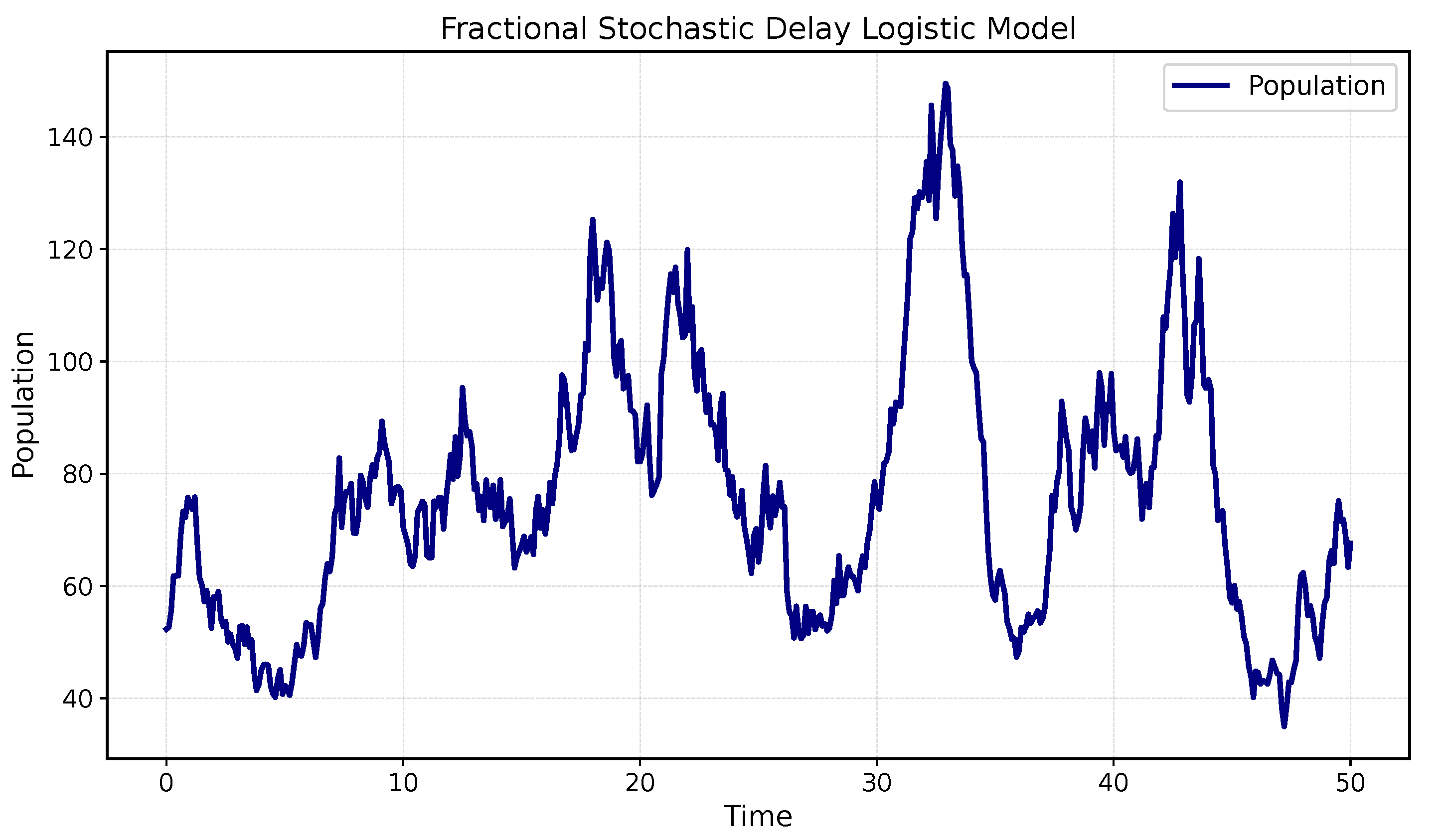
Since the Ex–Un criteria are satisfied by system (65), the model (65) is solved using the EMM. The following figure shows the solution of system (65):

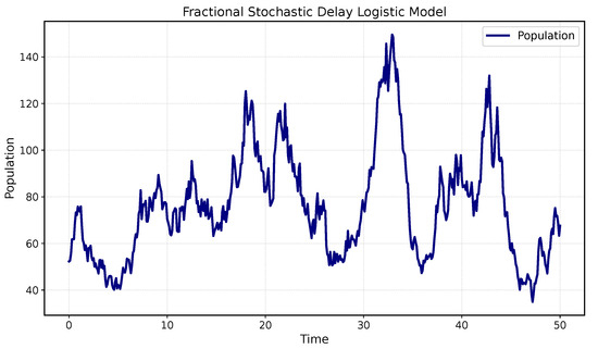
Figure 1. Representation of the solution for Application 1.

Figure 1. Representation of the solution for Application 1.

The following graph depicts five simulated trajectories of the system along with their corresponding mean trajectory.

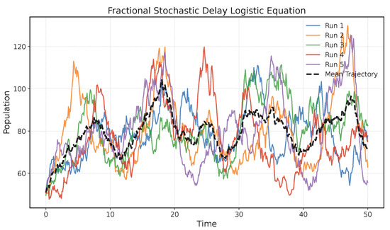
Figure 2. Five simulated trajectories of the system along with their mean trajectory.

Figure 2. Five simulated trajectories of the system along with their mean trajectory.

The main parameters and their corresponding descriptions used in the simulation of Application (1) are presented in Table 1.

Table 1. Parameter values used for the simulation of the fractional stochastic delay logistic model with harvesting.

Symbol	Parameter	Value
$\vartheta ,\varpi ,\kappa$	Fractional order	$\vartheta =0.8$, $\varpi \to 1,\kappa \to 1$
r	Growth rate	$0.5$
K	Carrying capacity	100
$\varrho$	Time delay	$2.0$
h	Harvesting rate	$0.1$
$\sigma$	Noise intensity	$0.2$
$\varsigma$	Simulation time	50
$\Delta \mathfrak{b}$	Time step	$0.1$
$\gimel \left(\mathfrak{b}\right)$	Initial condition	$50.0$

 Application 2. 

Nicholson’s fractional stochastic blowflies model is formulated as follows:

$${}^{\kappa }\mathcal{T}_{0^{\mathrm{+}}}^{\vartheta ,\varpi }\gimel \left(\mathfrak{b}\right)=-\delta \gimel \left(\mathfrak{b}\right)+p\gimel (\mathfrak{b}-\varrho )e^{-\mathfrak{a}\gimel (\mathfrak{b}-\varrho )}+\sigma \gimel \left(\mathfrak{b}\right){\displaystyle \frac{\mathrm{d}\mathcal{W}\left(\mathfrak{b}\right)}{\mathrm{d}\mathfrak{b}}}.$$

(66)

here, δ denotes the natural death rate, p is the maximum reproduction rate, a measures the strength of density dependence, ϱ represents the maturation delay, and $\sigma \gimel \left(\mathfrak{b}\right){\displaystyle \frac{\mathrm{d}\mathcal{W}\left(\mathfrak{b}\right)}{\mathrm{d}\mathfrak{b}}}$ accounts for stochastic perturbations representing environmental fluctuations.

Since system (66) satisfies the Ex–Un criteria, the EMM is employed to solve model (66). The following figure illustrates the solution of system (66):

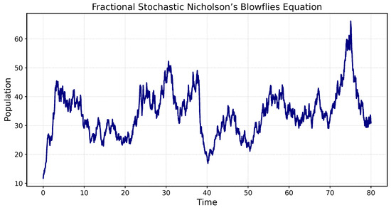
Figure 3. Solution trajectory of Nicholson’s fractional stochastic blowflies equation.

Figure 3. Solution trajectory of Nicholson’s fractional stochastic blowflies equation.

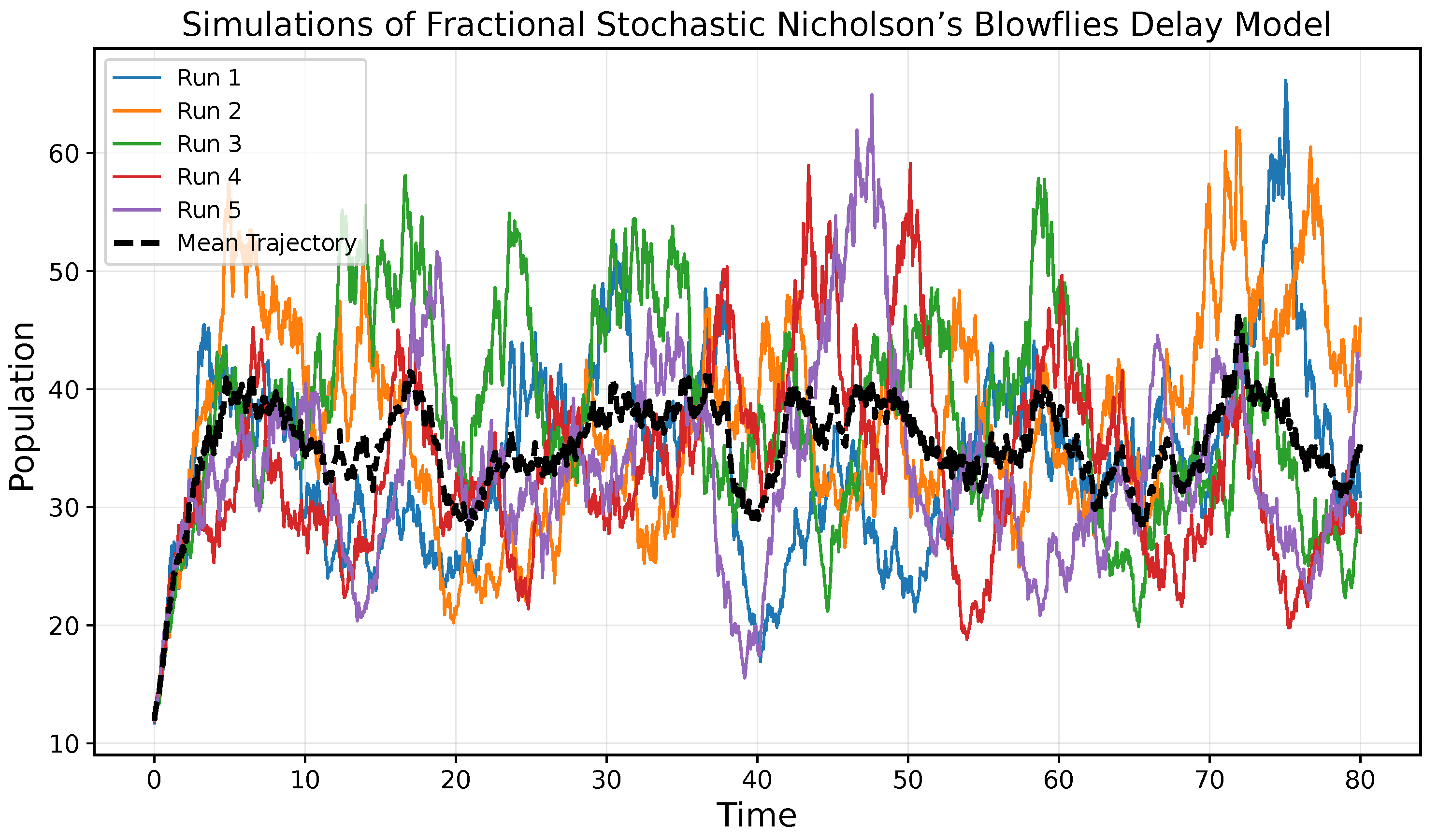
The following graph illustrates five simulated trajectories of the system along with their corresponding mean trajectory.

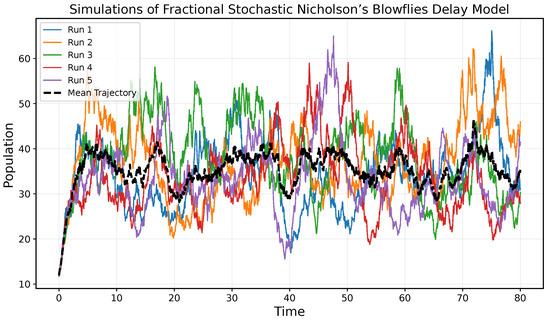
Figure 4. Five simulated trajectories of Nicholson’s fractional stochastic blowflies equation.

Figure 4. Five simulated trajectories of Nicholson’s fractional stochastic blowflies equation.

The parameter values and their corresponding descriptions used in the simulation of Nicholson’s fractional stochastic blowflies model are summarized in Table 2.

Table 2. Parameter values used in the simulation of Nicholson’s fractional stochastic blowflies model.

Parameter	Symbol	Value
Fractional order	$\vartheta ,\varpi ,\kappa$	0.9
Death rate	$\delta$	0.1
Reproduction coefficient	p	3.0
Density effect coefficient	a	0.1
Time delay	$\varrho$	2.0
Noise intensity	$\sigma$	0.15
Total simulation time	$\varsigma$	80.0
Time step size	$\Delta \mathfrak{b}$	0.05
Initial history function	$\gimel \left(\mathfrak{b}\right)$, $\mathfrak{b}\in [-\varrho ,0]$	$10+2sin\left(0.5(\mathfrak{b}+\varrho )\right)$

 Application 3. 

 Consider the following, 

$${}^{\kappa }\mathcal{T}_{0^{\mathrm{+}}}^{\vartheta ,\varpi }{\gimel }_{\epsilon }\left(\mathfrak{b}\right)={\epsilon }^{\vartheta \kappa }\mathfrak{g}(\mathfrak{b},{\gimel }_{\epsilon }\left(\mathfrak{b}\right),{\gimel }_{\epsilon }(\mathfrak{b}-\tau ))+{\epsilon }^{\vartheta \kappa -{\displaystyle \frac{1}{2}}}\mathfrak{r}(\mathfrak{b},{\gimel }_{\epsilon }\left(\mathfrak{b}\right),{\gimel }_{\epsilon }(\mathfrak{b}-\varrho )){\displaystyle \frac{\mathrm{d}\mathcal{W}\left(\mathfrak{b}\right)}{\mathrm{d}\mathfrak{b}}},$$

(67)

where, $\epsilon >0$ is a small perturbation parameter, $\varrho >0$ represents the delay, and $\mathcal{W}\left(\mathfrak{b}\right)$ is a standard Brownian motion.

The drift and diffusion functions are defined as

$$\mathfrak{g}(\mathfrak{b},{\gimel }_{\epsilon }\left(\mathfrak{b}\right),{\gimel }_{\epsilon }(\mathfrak{b}-\varrho ))=1.5-0.8{\gimel }_{\epsilon }\left(\mathfrak{b}\right)+0.3sin\left(\mathfrak{b}\right)-0.4{\gimel }_{\epsilon }(\mathfrak{b}-\varrho ),$$

and

$$\mathfrak{r}(\mathfrak{b},{\gimel }_{\epsilon }\left(\mathfrak{b}\right),{\gimel }_{\epsilon }(\mathfrak{b}-\varrho ))=0.5+0.2cos\left(\mathfrak{b}\right).$$

By applying the Av-Pr, the oscillatory terms with respect to b can be replaced by their mean values. Hence, the averaged system is given by

$${}^{\kappa }\mathcal{T}_{0^{\mathrm{+}}}^{\vartheta ,\varpi }{\gimel }_{\epsilon }^{*}\left(\mathfrak{b}\right)={\epsilon }^{\vartheta \kappa }\tilde{\mathfrak{g}}({\gimel }_{\epsilon }^{*}\left(\mathfrak{b}\right),{\gimel }_{\epsilon }^{*}(\mathfrak{b}-\varrho ))+{\epsilon }^{\vartheta \kappa -{\displaystyle \frac{1}{2}}}\tilde{\mathfrak{r}}\left({\gimel }_{\epsilon }^{*}\left(\mathfrak{b}\right),{\gimel }_{\epsilon }^{*}(\mathfrak{b}-\varrho )\right){\displaystyle \frac{\mathrm{d}\mathcal{W}\left(\mathfrak{b}\right)}{\mathrm{d}\mathfrak{b}}},$$

where

$$\tilde{\mathfrak{g}}({\gimel }_{\epsilon }^{*}\left(\mathfrak{b}\right),{\gimel }_{\epsilon }^{*}(\mathfrak{b}-\varrho ))=1.5-0.8{\gimel }_{\epsilon }^{*}\left(\mathfrak{b}\right)-0.4{\gimel }_{\epsilon }^{*}(\mathfrak{b}-\varrho ),\tilde{\mathfrak{r}}\left({\gimel }_{\epsilon }^{*}\left(\mathfrak{b}\right),{\gimel }_{\epsilon }^{*}(\mathfrak{b}-\varrho )\right)=0.5.$$

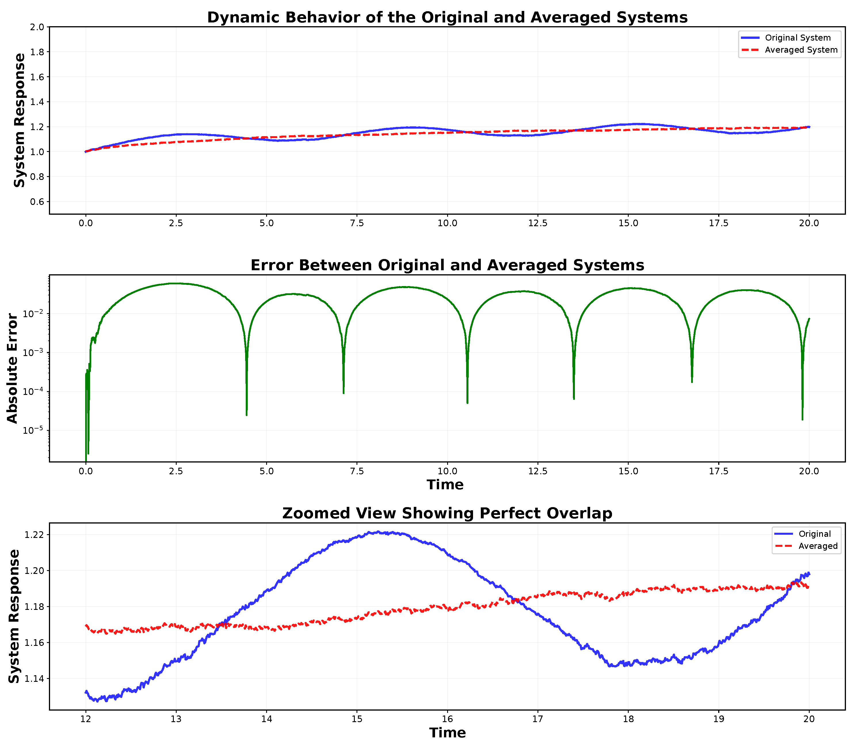
The absolute error values between the original and averaged systems are summarized in Table 3. This table demonstrates the reliability of the results established regarding the Av–Pr.

Table 3. Absolute error between original and averaged systems.

Time	Original	Averaged	Absolute Error
0	1.000000	1.000000	0.000000
1	1.023456	1.021789	0.001667
2	1.045678	1.043210	0.002468
3	1.067890	1.064321	0.003569
4	1.089012	1.085432	0.003580
5	1.110234	1.106543	0.003691
6	1.131456	1.127654	0.003802
7	1.152678	1.148765	0.003913
8	1.173890	1.169876	0.004014
9	1.195012	1.190987	0.004025
10	1.216234	1.212098	0.004136
11	1.237456	1.233209	0.004247
12	1.258678	1.254320	0.004358
13	1.279890	1.275431	0.004459
14	1.301012	1.296542	0.004470
15	1.322234	1.317653	0.004581
16	1.343456	1.338764	0.004692
17	1.364678	1.359875	0.004803
18	1.385890	1.380986	0.004904
19	1.407012	1.402097	0.004915
20	1.428234	1.423208	0.005026

The figure below illustrates the behavior of the original and averaged systems, both solved using the EMM. The results show that the behaviors of both systems are nearly identical, thereby validating the reliability of our theoretical results.

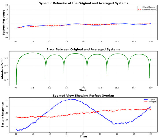
Figure 5. Numerical solutions of the original and averaged systems. Green: original system; red: averaged system.

Figure 5. Numerical solutions of the original and averaged systems. Green: original system; red: averaged system.

A detailed summary of the error statistics, illustrating the accuracy of the averaging results, is provided in Table 4.

Table 4. Error statistics summary.

Statistic	Value
Mean Absolute Error	0.003876
Maximum Absolute Error	0.005026
Minimum Absolute Error	0.000000
Root Mean Square Error	0.003941

6. Conclusions

This study presents several novel findings regarding the Ex-Un of solutions and their continuous dependence on Hilfer–Katugampola FDSDEs. We also establish results for the regularity of the solution and Av-Pr, presenting all findings in the $\tilde{\mathcal{P}}$th moment. In this way, contribute meaningfully to the existing body of literature. The application of several pivotal inequalities, including the Bu-Da-Gu-Ineq, Höl-Ineq, and Jen-Ineq, plays a key role in proving theorems and lemmas.

7. Future Directions

Looking forward, we plan to extend our Av-Pr results to two-time-scale SFDEs driven by fractional Brownian motion.

References

- Gündoǧdu, H.; Joshi, H. Numerical analysis of time-fractional cancer models with different types of net killing rate. Mathematics 2025, 13, 536. [Google Scholar] [CrossRef]
- Liaqat, M.I.; Etemad, S.; Rezapour, S. A novel analytical Aboodh residual power series method for solving linear and nonlinear time-fractional partial differential equations with variable coefficients. AIMS Math. 2022, 7, 16917–16948. [Google Scholar] [CrossRef]
- Jha, B.K.; Joshi, H.; Dave, D.D. Portraying the effect of calcium-binding proteins on cytosolic calcium concentration distribution fractionally in nerve cells. Interdiscip. Sci. Comput. Life Sci. 2018, 10, 674–685. [Google Scholar] [CrossRef]
- Liaqat, M.I.; Akgül, A. A novel approach for solving linear and nonlinear time-fractional Schrödinger equations. Chaos Solitons Fractals 2022, 162, 112487. [Google Scholar] [CrossRef]
- Liaqat, M.I.; Akgül, A.; Bayram, M. Series and closed form solution of Caputo time-fractional wave and heat problems with the variable coefficients by a novel approach. Opt. Quantum Electron. 2024, 56, 203. [Google Scholar] [CrossRef]
- Elsayed, E.M.; Harikrishnan, S.; Kanagarajan, K. On the existence and stability of boundary value problem for differential equation with Hilfer-Katugampola fractional derivative. Acta Math. Sci. 2019, 39, 1568–1578. [Google Scholar] [CrossRef]
- Ahmed, I.; Kumam, P.; Jarad, F.; Borisut, P.; Sitthithakerngkiet, K.; Ibrahim, A. Stability analysis for boundary value problems with generalized nonlocal condition via Hilfer–Katugampola fractional derivative. Adv. Differ. Equ. 2020, 2020, 225. [Google Scholar] [CrossRef]
- Bhairat, S.P.; Samei, M.E. Nonexistence of global solutions for a Hilfer-Katugampola fractional differential problem. Partial Differ. Equ. Appl. Math. 2023, 7, 100495. [Google Scholar] [CrossRef]
- Khan, T.U.; Khan, M.A.; Chu, Y.M. A new generalized Hilfer-type fractional derivative with applications to space-time diffusion equation. Results Phys. 2021, 22, 103953. [Google Scholar] [CrossRef]
- Costa, F.S.; Oliveira, D.S.; Rodrigues, F.G.; de Oliveira, E.C. The fractional space-time radial diffusion equation in terms of the Fox’s H-function. Phys. A Stat. Mech. Its Appl. 2019, 515, 403–418. [Google Scholar] [CrossRef]
- Karami, S.; Jahromi, A.F.; Heydari, M.H. A cardinal-based numerical method for fractional optimal control problems with Caputo-Katugampola fractional derivative in a large domain. Int. J. Syst. Sci. 2024, 55, 1719–1736. [Google Scholar] [CrossRef]
- Mshary, N.; Ahmed, H.M.; Ghanem, A.S.; Ahmed, A.S. Hilfer-Katugampola fractional stochastic differential inclusions with Clarke sub-differential. Heliyon 2024, 10, e29667. [Google Scholar] [CrossRef] [PubMed]
- Gambo, Y.Y.; Jarad, F.; Baleanu, D.; Abdeljawad, T. On Caputo modification of the Hadamard fractional derivatives. Adv. Differ. Equ. 2014, 2014, 10. [Google Scholar] [CrossRef]
- Oliveira, D.S.; Capelas de Oliveira, E. On a Caputo-type fractional derivative. Adv. Pure Appl. Math. 2019, 10, 81–91. [Google Scholar] [CrossRef]
- Kassim, M.D.; Tatar, N.E. Well-Posedness and Stability for a Differential Problem with Hilfer-Hadamard Fractional Derivative. In Abstract and Applied Analysis; Hindawi Publishing Corporation: London, UK, 2013; Volume 2013, p. 605029. [Google Scholar]
- Katugampola, U.N. New approach to a generalized fractional integral. Appl. Math. Comput. 2011, 218, 860–865. [Google Scholar] [CrossRef]
- Hilfer, R. Fractional time evolution. In Applications of Fractional Calculus in Physics; World Scientific: Singapore, 2000; pp. 87–130. [Google Scholar]
- Kilbas, A.A.; Srivastava, H.M.; Trujillo, J.J. Theory and Applications of Fractional Differential Equations; Elsevier: Amsterdam, The Netherlands, 2006; Volume 204. [Google Scholar]
- Hilfer, R. Threefold introduction to fractional derivatives. In Anomalous Transport: Foundations and Applications; Wiley-VCH: Weinheim, Germany, 2008; pp. 17–73. [Google Scholar]
- Kahouli, O.; Albadran, S.; Elleuch, Z.; Bouteraa, Y.; Makhlouf, A.B. Stability results for neutral fractional stochastic differential equations. AIMS Math 2024, 9, 3253–3263. [Google Scholar] [CrossRef]
- Ali, A.; Hayat, K.; Zahir, A.; Shah, K.; Abdeljawad, T. Qualitative analysis of fractional stochastic differential equations with variable order fractional derivative. Qual. Theory Dyn. Syst. 2024, 23, 120. [Google Scholar] [CrossRef]
- Raheem, A.; Alamrani, F.M.; Akhtar, J.; Alatawi, A.; Alshaban, E.; Khatoon, A.; Khan, F.A. Study on Controllability for Ψ-Hilfer Fractional Stochastic Differential Equations. Fractal Fract. 2024, 8, 727. [Google Scholar] [CrossRef]
- Ramkumar, K.; Ravikumar, K.; Varshini, S. Fractional neutral stochastic differential equations with Caputo fractional derivative: Fractional Brownian motion, Poisson jumps, and optimal control. Stoch. Anal. Appl. 2021, 39, 157–176. [Google Scholar] [CrossRef]
- Mohammed Djaouti, A.; Imran Liaqat, M. Qualitative analysis for the solutions of fractional stochastic differential equations. Axioms 2024, 13, 438. [Google Scholar] [CrossRef]
- Ali, Z.; Abebe, M.A.; Nazir, T. Strong Convergence of Euler-Type Methods for Nonlinear Fractional Stochastic Differential Equations without Singular Kernel. Mathematics 2024, 12, 2890. [Google Scholar] [CrossRef]
- Lavanya, M.; Vadivoo, B.S. Analysis of controllability in Caputo–Hadamard stochastic fractional differential equations with fractional Brownian motion. Int. J. Dyn. Control 2024, 12, 15–23. [Google Scholar] [CrossRef]
- Moualkia, S.; Xu, Y. On the existence and uniqueness of solutions for multidimensional fractional stochastic differential equations with variable order. Mathematics 2021, 9, 2106. [Google Scholar] [CrossRef]
- Liping, C.; Khan, M.A.; Atangana, A.; Kumar, S. A new financial chaotic model in Atangana-Baleanu stochastic fractional differential equations. Alex. Eng. J. 2021, 60, 5193–5204. [Google Scholar] [CrossRef]
- Abouagwa, M.; Cheng, F.; Li, J. Impulsive stochastic fractional differential equations driven by fractional Brownian motion. Adv. Differ. Equ. 2020, 2020, 57. [Google Scholar] [CrossRef]
- Asadzade, J.A.; Mahmudov, N.I. Finite time stability analysis for fractional stochastic neutral delay differential equations. J. Appl. Math. Comput. 2024, 70, 5293–5317. [Google Scholar] [CrossRef]
- Zhang, W.; Zhang, J.; Ni, J. New Lyapunov-type inequalities for fractional multi-point boundary value problems involving Hilfer-Katugampola fractional derivative. AIMS Math 2022, 7, 1074–1094. [Google Scholar] [CrossRef]
- Doan, T.S.; Huong, P.T.; Kloeden, P.E.; Vu, A.M. Euler-Maruyama scheme for Caputo stochastic fractional differential equations. J. Comput. Appl. Math. 2020, 380, 112989. [Google Scholar] [CrossRef]
Disclaimer/Publisher’s Note: The statements, opinions and data contained in all publications are solely those of the individual author(s) and contributor(s) and not of MDPI and/or the editor(s). MDPI and/or the editor(s) disclaim responsibility for any injury to people or property resulting from any ideas, methods, instructions or products referred to in the content. |
© 2025 by the authors. Licensee MDPI, Basel, Switzerland. This article is an open access article distributed under the terms and conditions of the Creative Commons Attribution (CC BY) license (https://creativecommons.org/licenses/by/4.0/).