Abstract
Mean Shift is a flexible, non-parametric clustering algorithm that identifies dense regions in data through gradient ascent on a kernel density estimate. Its ability to detect arbitrarily shaped clusters without requiring prior knowledge of the number of clusters makes it widely applicable across diverse domains. However, its quadratic computational complexity restricts its use on large or high-dimensional datasets. Numerous acceleration techniques, collectively referred to as Fast Mean Shift strategies, have been developed to address this limitation while preserving clustering quality. This paper presents a systematic theoretical analysis of these strategies, focusing on their computational impact, pairwise combinability, and mapping onto distinct stages of the Mean Shift pipeline. Acceleration methods are categorized into seed reduction, neighborhood search acceleration, adaptive bandwidth selection, kernel approximation, and parallelization, with their algorithmic roles examined in detail. A pairwise compatibility matrix is proposed to characterize synergistic and conflicting interactions among strategies. Building on this analysis, we introduce a decision framework for selecting suitable acceleration strategies based on dataset characteristics and computational constraints. This framework, together with the taxonomy, combinability analysis, and scenario-based recommendations, establishes a rigorous foundation for understanding and systematically applying Fast Mean Shift methods.
Keywords:
Mean Shift clustering; Fast Mean Shift; acceleration strategies; optimization techniques; kernel density estimation; theoretical analysis; algorithmic complexity; decision framework; high-dimensional data; neighborhood search; adaptive bandwidth selection; parallelization MSC:
62H30; 62G07; 68W40; 90C59
1. Introduction
Mean Shift [1] is a powerful, non-parametric clustering method which is widely appreciated for its flexibility in identifying modes or dense regions of a data distribution in complex and multimodal feature spaces [2]. At its core, Mean Shift is conceived as a deterministic, iterative procedure that treats the data points as an empirical probability density function and iteratively shifts each data point towards the densest area in its vicinity until it reaches a mode [3]—a point where the local density is maximized. This process can be visualized as hill climbing on a density surface, where each data point moves uphill until it reaches a peak, or a mode. All data points that converge to the same mode are then considered part of the same cluster. This methodology fundamentally reframes the objective of clustering. Rather than approaching clustering task as a problem of finding an optimal partitioning of the data according to some global cost function, Mean Shift treats it as a deterministic problem of discovering the topological features of the feature space itself, e.g., seeking to reveal the structure that is inherently present in the data’s density landscape.
A principal advantage of Mean Shift approach is its non-parametric and deterministic nature. Unlike many other popular clustering techniques such as k-means [4,5], Mean Shift does not require prior knowledge of the number of clusters, making it a valuable tool for discovering the natural underlying structure within a dataset. Its ability to identify clusters of arbitrary shapes and its robustness to outliers further enhance its utility. It is not limited to finding spherical clusters and can identify complex and elongated structures in the data. Outliers, being in low-density regions, are less likely to form their own significant clusters and have a minimal impact on the final clustering result.
The Mean Shift clustering method is widely used in image processing tasks such as segmentation and object tracking [6,7,8,9,10], as well as in pattern recognition [1,3,11,12]. The algorithm has also been applied to high-dimensional texture classification [2] and in the analysis and visualization of complex datasets [13,14]. In data science, it plays a role in feature space analysis [12], density estimation [15], and data sharpening [15]. Biomedical domains benefit from Mean Shift in applications such as disease prediction from metagenomic data [14] and brain tumor detection in MRI images [8]. It has also been incorporated into speaker and biometric verification systems through score normalization [16,17,18], and in image retrieval via feature normalization [19]. These developments, alongside theoretical advancements [1,3], have made Mean Shift as a versatile and evolving tool in modern data analysis and machine learning.
2. Standard Mean Shift Algorithm
The pseudocode presented in Algorithm 1 outlines the standard Mean Shift clustering procedure, as commonly implemented in the literature. It consists of three primary stages: mode seeking, mode consolidation, and cluster assignment. The process begins by creating a working copy Y of the original dataset , where each point represents a data instance that serves as a seed for mode discovery during the Mean Shift clustering process. An example dataset is illustrated in Figure 1a.


Figure 1.
Illustration of the Mean Shift clustering process. Subfigure (a) shows the initial distribution of data points, while subfigure (b) visualizes how each point follows a unique convergence trajectory toward a mode. The trajectory of each individual point during the iterative shifting process is shown in a distinct color, illustrating how points move along different paths toward their respective local density maxima.
| Algorithm 1: Standard Mean Shift Clustering Algorithm |
 |
The algorithm employs kernel density estimation (KDE) [1,15,20] to construct a continuous approximation of the underlying data distribution. The estimated probability density function (PDF) at any location x is given by
where is a radially symmetric kernel function, is the bandwidth, and d is the dimensionality of the feature space. KDE enables gradient-based optimization by smoothing the discrete distribution of data points, allowing for meaningful definitions of local maxima (modes). Mean Shift interprets clustering as a gradient ascent procedure on this estimated density surface [3,12]. Figure 2a shows the kernel density surface generated by Mean Shift using a standard bandwidth, based on the example dataset in Figure 1a. The algorithm iteratively performs gradient ascent on this surface to locate local maxima, which correspond to cluster modes. These modes are depicted as black points in Figure 1b.
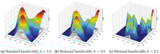
Figure 2.
Effect of varying bandwidth values on the shape of the kernel density surface for different bandwidth choices. Red indicates the maximal possible density, dark blue corresponds to the minimal possible density, and intermediate colors represent intermediate density values.
For each point , the algorithm iteratively computes the Mean Shift vector:
which indicates the direction of maximum increase in the estimated density. The update rule is simply
and the iteration continues until convergence is reached, defined by
where is a small positive threshold. At this point, is considered to have reached a mode. Mean Shift is guaranteed to converge because it performs a gradient ascent on a smooth, bounded kernel density estimate, ensuring each update increases the density until reaching a stationary point.
After all points in Y have converged, the algorithm performs mode consolidation by merging nearby modes. Specifically, any pair of converged points and satisfying
are merged into a single representative cluster center. This reduces redundancy and ensures that only distinct, well-separated modes are retained [2].
In the final cluster assignment stage, each original data point is assigned to the cluster corresponding to the mode it converged to:
where is the set of unique cluster centers obtained after mode merging.
This formulation highlights the deterministic, gradient-ascent nature of the algorithm and its reliance on kernel density estimation to uncover the topological structure of the data [1,2,3,12].
In practice, a common choice for the kernel function is the Gaussian kernel:
where . This kernel provides smooth, distance-weighted contributions from neighboring points, emphasizing closer ones. The bandwidth h governs the scale of smoothing and has a significant influence on clustering resolution. While the kernel shape is generally less critical, an appropriately chosen bandwidth is essential for meaningful results. The effect of varying bandwidth values on the shape of the kernel density surface is illustrated in Figure 2, using the example dataset shown in Figure 1a. With a standard bandwidth (Figure 2a), the surface is smooth and captures the overall structure of the data, resulting in clearly defined and well-separated modes. As the bandwidth is reduced (Figure 2b), the surface becomes more detailed, but also more sensitive to local variations, potentially introducing spurious modes. When the bandwidth is minimal (Figure 2c), the surface becomes overly fragmented, forming sharp peaks around individual points and leading to excessive, noisy clustering.
Mean Shift is widely regarded as a nonparametric clustering algorithm because it does not require the user to predefine the number of clusters, and it derives cluster structure directly from the data distribution through mode-seeking. Unlike parametric methods such as k-means or Gaussian Mixture Models (GMMs), which assume a fixed number of clusters or specific parametric forms, Mean Shift adapts to the underlying data density without making strong model assumptions. However, in practical implementations, the algorithm still depends on several important parameters that influence its behavior and outcomes. These include the choice of kernel function K, the bandwidth parameter h that controls the kernel scale, the convergence threshold used to stop iterative updates, and the merging threshold for consolidating similar modes. While these parameters do not define the number of clusters directly, they significantly affect the resolution and stability of the clustering result. Thus, although Mean Shift is nonparametric in theory, careful tuning of these parameters is essential in practice for effective and interpretable clustering.
2.1. Convergence Threshold
The convergence threshold determines when the Mean Shift updates are considered to have stabilized for a given point. A suitable value should be small enough to ensure that the algorithm accurately locates local density maxima, but not so small as to cause unnecessary computation or sensitivity to noise. In practice, is often chosen relative to the bandwidth h, such as or , depending on the scale and precision requirements of the data. Smaller values yield higher accuracy but increase the number of iterations; larger values may speed up convergence but risk premature stopping. Adaptive selection strategies based on data scale or dynamic step size control can also be employed for improved efficiency.
Comparing Mean Shift to DBSCAN [21], which is another popular density-based clustering algorithm, both methods can identify clusters of arbitrary shapes and are robust to outliers. The primary difference lies in how they handle density. DBSCAN explicitly identifies and labels noise points, whereas Mean Shift manages noise implicitly through its bandwidth parameter. Additionally, DBSCAN requires two parameters (epsilon and minimum points), while Mean Shift primarily depends on a single parameter, the bandwidth.
2.2. Preliminary Data Normalization
Preliminary data normalization is not strictly obligatory for standard Mean Shift clustering when a fixed bandwidth parameter h is used, as the algorithm can operate directly on the original data. However, it is strongly recommended in most practical applications, particularly when the dataset contains features with different units or varying scales. Without normalization, Euclidean distance computations may be dominated by features with larger variances, potentially distorting the kernel density estimation and leading to biased clustering results. A common approach is to apply standardization, where each feature is transformed to have zero mean and unit variance, , with and denoting the mean and standard deviation of feature j. Alternatively, min–max normalization can be used to rescale features to the interval, . Such normalization makes the bandwidth parameter h more interpretable and consistent across features, simplifying parameter tuning and improving the stability and reliability of the clustering process.
2.3. Computational Complexity of the Standard Mean Shift Algorithm
We analyze the computational complexity of the standard Mean Shift algorithm under the uniform-cost model when each arithmetic operation and memory access requires constant time. According to (2), in each iteration, for every point , the standard Mean Shift algorithm computes the kernel-weighted mean shift vector , which involves evaluating n kernel values and n distance computations in . Computing the squared Euclidean distance [22] between two d-dimensional vectors requires operations, and evaluating the kernel adds only constant overhead. Therefore, the cost of updating one point is
Since all n points are updated independently within each iteration, the total per-iteration computational cost is
This quadratic scaling with respect to n arises from the exhaustive pairwise computations required to evaluate the kernel density estimate exactly. The memory complexity of the standard algorithm is , as it stores the dataset and intermediate results for all n points. This analysis is consistent with classical theoretical results [1,3,12], which describe Mean Shift as an exact gradient ascent on a kernel density estimate, inherently involving all pairwise interactions at each iteration.
To mitigate these computational challenges, various acceleration strategies have been developed. These include approximate methods and spatial data structures that restrict computations to local neighborhoods within the bandwidth h, as well as parallelization and convergence acceleration techniques that reduce runtime without compromising clustering accuracy. The following sections examine these strategies in detail and analyze their theoretical impact on the efficiency of Mean Shift clustering.
3. Analysis of Optimization Strategies for Fast Mean Shift Clustering
The computational complexity of the standard Mean Shift algorithm presents significant challenges for practical applications, particularly with large-scale and high-dimensional datasets. To address these limitations, several optimization strategies have been proposed in the literature, collectively known as Fast Mean Shift methods. The primary goal of Fast Mean Shift methods is to reduce computational complexity and enhance scalability without sacrificing clustering accuracy significantly. In the following sections, we will analyze the core ideas behind these optimization strategies, focusing on their algorithmic principles. Research on Fast Mean Shift has progressed along four main axes: (i) spatial indexing and kernel approximation, (ii) adaptive bandwidth and convergence acceleration, (iii) neighborhood pruning and early stopping, and (iv) parallel implementations and hybrids.
3.1. Parallel Mean Shift Clustering
The computational cost of the standard Mean Shift algorithm was derived in Section 2.3, where Equation (9) showed that the total per-iteration complexity scales as due to the exhaustive pairwise computations required to evaluate the kernel density estimate. This quadratic growth makes the algorithm computationally expensive for large-scale and high-dimensional datasets, motivating the use of parallelization strategies to improve scalability.
Parallel processing addresses this bottleneck by distributing the workload across multiple processing units [23]. The Mean Shift algorithm is inherently parallelizable because the mode-seeking trajectory of each data point is independent of all others [6]. This property makes it particularly suitable for acceleration on modern multi-core CPUs (Central Processing Units) and many-core GPUs (Graphics Processing Units), especially when applied to large datasets [24]. In the parallel setting, the n independent update operations are partitioned across p processing units. Assuming balanced workload distribution and negligible synchronization overhead, each processor updates roughly points per iteration, with each update still incurring work, as in the sequential case. Consequently, the total per-iteration cost becomes
Under standard parallel computation models, this yields a near-linear speedup in p, substantially improving scalability on modern architectures and reducing wall-clock time while leaving the overall amount of computation unchanged. In practice, deviations from this ideal behavior may arise due to communication overhead, memory bandwidth saturation, or load imbalance [25].
Algorithm 2 presents a parallelized version of the Mean Shift clustering algorithm, in which the mode-seeking and cluster assignment steps are executed concurrently across data points to improve scalability on modern parallel hardware.
| Algorithm 2: Parallel Mean Shift Clustering |
 |
In CPU-based parallel implementations, the dataset is divided across multiple threads, each independently performing Mean Shift updates on a subset of data points. Thread-safe data structures are employed to handle mode consolidation and cluster label assignment. Performance can be further improved using efficient memory access patterns and cache-aware optimizations [23,26].
GPUs are also highly effective for accelerating Mean Shift due to their massively parallel architecture [6,23]. GPU-based implementations [27] exploit this architecture to compute kernel evaluations and update steps concurrently for thousands of points [24,28].
While parallelism significantly improves scalability, it also introduces several implementation challenges. In particular, some data points may require more iterations to converge than others, leading to load imbalance. Therefore, effective load balancing strategies are essential to maintain overall computational efficiency.
3.2. Seed Point Sampling
A fundamental characteristic of the standard Mean Shift algorithm is that each data point in the dataset acts as an initial seed for mode seeking. While this exhaustive seeding strategy ensures that all modes are detected with high fidelity [12], it also significantly contributes to the overall computational burden: n seed points are shifted over T iterations, each incurring neighborhood queries and kernel evaluations, resulting in the quadratic complexity analyzed in Section 2.3. For large datasets, especially when many points are located in dense regions and converge to the same modes, this approach leads to redundant computations [6,29].
Seed point sampling addresses this inefficiency by selecting a reduced subset of representative seed points, with , from which the Mean Shift trajectories are initiated [30,31,32,33]. Since the purpose of seeding is to identify the set of modes, rather than to individually trace every data point’s trajectory, it is often sufficient to launch gradient ascent from a carefully chosen subset that adequately covers the data distribution. After the mode locations have been determined using the sampled seeds, the remaining points can be assigned to clusters via a single nearest-mode lookup, dramatically reducing computational cost.
Seed point sampling alters the standard Mean Shift pipeline in two key ways:
- Seed selection. Instead of initializing a trajectory at every data point, a reduced set with is chosen using a suitable sampling strategy.
- Cluster assignment. After modes are found from the sampled seeds, the remaining data points are assigned to the nearest mode in the final set of cluster centers C, typically using efficient spatial indexing.
All other steps of the algorithm (i.e., mean shift updates on seeds, mode merging) remain unchanged.
This procedure preserves the structure of the Mean Shift algorithm but greatly reduces the number of gradient ascent trajectories that need to be computed. The final cluster assignments are obtained via a single nearest-mode search, typically using efficient spatial data structures such as k-d trees or ball trees to achieve query time.
3.2.1. Sampling Strategies
Several strategies have been proposed for selecting the seed subset S:
- Uniform random sampling. Randomly selecting a small subset of points can drastically reduce computational cost while maintaining accuracy, even with very few seeds per frame [31].
- Iterative re-sampling. The active point set can be dynamically updated during iterations, simplifying the dataset while preserving convergence accuracy and accelerating clustering [30].
- Structured or slice-based sampling. Seeds can be placed only in candidate regions (e.g., line segments) using slice sampling, focusing computation where it is most needed [32].
- Task-guided sparse sampling. In application-specific settings, computational cost can be controlled by applying mean shift only to a sparse subset of points guided by auxiliary information (e.g., audio cues) [33].
- Density-aware sampling. Seeds may be drawn with probabilities proportional to local density, or selected using farthest-point or k-means++ seeding, to improve mode coverage while minimizing redundancy [12].
3.2.2. Computational Impact of Seed Point Sampling
Let be the number of selected seeds. The cost of the mode-seeking stage is reduced from to , because only the s seeds undergo iterative updates, while each update still involves n reference points for kernel evaluation. When , this yields a substantial reduction in total runtime. The subsequent mode consolidation step operates on s converged points, costing , which is negligible when s is small. Finally, the cluster assignment step for all n points requires time if spatial indexing is used for nearest-mode lookup, with .
Empirical studies confirm these improvements. Leung and Gong [31] achieved real-time tracking with drastic sampling reductions. Huimin et al. [30] reported marked acceleration from iterative re-sampling. Nieto et al. [32] demonstrated that slice-based seed placement improved both accuracy and speed for line detection. Kılıç et al. [33] showed similar benefits in tracking by sparsifying particle sets.
3.2.3. Practical Considerations for Seed Point Sampling
The choice of s and the sampling strategy must balance efficiency and clustering accuracy. If s is too small or poorly distributed, some modes may be missed, leading to under-segmentation. Stratified, task-aware, or density-aware sampling mitigates this risk, especially in heterogeneous datasets. A practical heuristic is to select for small constants c and (e.g., ), ensuring that all major modes are likely to be sampled with high probability.
3.3. Early Stopping Criteria
Rather than updating every point to full convergence, it is possible to introduce density thresholding or early stopping criteria [6,27] for Mean Shift, terminating the update process when the local density or point trajectory stabilizes sufficiently. This strategy reduces unnecessary iterations for points that have effectively reached their target modes, improving computational efficiency without materially affecting clustering results. Zhao et al. [6] further demonstrate that combining early stopping with GPU acceleration yields substantial runtime improvements while maintaining clustering quality on large-scale datasets.
3.3.1. Density-Based Early Stopping
One simple criterion relies on monitoring the estimated kernel density at each point during the Mean Shift iterations. Recall that Mean Shift performs gradient ascent on the estimated kernel density surface . Once a point has reached a region where the relative increase in density between successive iterations falls below a specified tolerance , the update process can be stopped:
where denotes the position of point at iteration t. Typical choices for range from to , depending on the desired trade-off between speed and precision. This criterion prevents spending iterations on marginal density improvements that have negligible effect on final mode assignment.
3.3.2. Trajectory-Based Early Stopping
Another approach exploits the observation that, in later iterations, point trajectories become nearly stationary and move along short, repetitive paths toward their final modes. If the displacement between successive iterations falls below a threshold for several consecutive steps, the trajectory can be truncated early [6,23]. Specifically, early stopping is triggered when
for s consecutive iterations, where is typically set to a fraction of the bandwidth h (e.g., to ). The parameter s provides robustness against transient plateaus or oscillations. This criterion is particularly effective in dense regions, where points converge rapidly to modes and additional iterations yield diminishing returns.
3.3.3. Computational Benefits of Early Stopping
Early stopping criteria reduce the number of Mean Shift iterations required per point by preventing redundant updates once local convergence is effectively achieved. If T denotes the number of iterations required by the standard algorithm and the number with early stopping, then, typically, for points in dense regions, which constitute the majority in many practical datasets. As a result, the total runtime can be reduced substantially, especially when combined with neighborhood pruning or approximate neighbor search methods.
Let denote the number of active (non-stopped) points at iteration t. In the standard algorithm, for all t, whereas with early stopping, decreases monotonically as points terminate their updates at different times. Let denote the maximum number of iterations performed by any point under early stopping. The total computational work is then proportional to , which can be significantly smaller than the operations required by the standard algorithm. This effect can be summarized by replacing the standard runtime with
where represents the effective number of iterations aggregated over all points.
Empirical studies [6,27] show that early stopping can reduce runtime by 20– on large image segmentation and high-dimensional clustering tasks, with negligible impact on clustering accuracy. Moreover, multilevel early stopping strategies further enhance computational efficiency by combining different stopping thresholds across iterations. This approach is particularly effective in GPU-accelerated frameworks [6], where early-stopped points no longer consume processing cycles, thereby improving resource utilization and enabling dynamic workload balancing for additional speedups in practice.
3.3.4. Practical Considerations of Early Stopping
Early stopping parameters should be chosen carefully to balance speed and accuracy. A very large or may cause points to stop prematurely, potentially merging distinct nearby modes. Conversely, overly strict thresholds may offer little benefit. A recommended strategy is to set to approximately of the kernel bandwidth h and to , then adjust based on pilot runs. Combining trajectory-based and density-based criteria often yields the most robust and efficient performance in practice.
3.4. Blurring Mean Shift
The Blurring Mean Shift (BMS) algorithm [3,34] is a variant of the standard Mean Shift procedure in which the entire dataset is updated at each iteration, progressively “blurring” the data distribution toward its modes. BMS has been widely studied and extended in various contexts, including image segmentation [35], manifold denoising [36], and clustering of structured data [37]. In contrast to the classical Mean Shift algorithm, where only a set of query points Y is shifted while the original dataset X remains fixed, the BMS algorithm applies the mean shift update directly to all points in X at each iteration. This leads to a collective evolution of the data cloud, gradually collapsing toward the set of modes and often accelerating convergence.
Formally, starting from the original dataset , the BMS algorithm applies the Mean Shift update to each point in to obtain the next iteration :
Equivalently, this can be written as a gradient ascent on the kernel density estimate where the support points themselves are moved toward higher density regions. All data points, thus, participate in both defining and evolving the density landscape at each iteration. Over successive iterations, the distribution of points becomes progressively sharper around the modes, resembling a blurring process that concentrates mass at the maxima of the kernel density estimate.
3.4.1. Convergence Properties of BMS
Unlike the standard Mean Shift, where convergence is established pointwise along gradient ascent trajectories, BMS updates the entire dataset simultaneously and exhibits global convergence in the sense that all points eventually collapse into a finite set of distinct modes [3,34]. Rigorous convergence and consistency results for BMS were later established in [38], providing a solid theoretical foundation for its asymptotic behavior. Moreover, the BMS update is contractive for commonly used kernels such as the Gaussian, ensuring that the sequence converges monotonically in terms of density increase. The global evolution of the dataset toward modes accelerates the blurring process, often reducing the required number of iterations. Its ability to sharpen and concentrate the data distribution has also been exploited as a preprocessing step for downstream tasks such as classification and feature extraction.
3.4.2. Computational Impact of BMS
The per-iteration computational complexity of BMS remains on the same order as that of the standard Mean Shift algorithm. In its naive Mean Shift implementation, each point interacts with all others during the update step, resulting in a per-iteration complexity of , where n is the number of data points and d is the dimensionality of the feature space. However, unlike classical Mean Shift, BMS updates the entire dataset at each iteration, which induces a progressive sharpening of the underlying density landscape. This accelerated evolution toward well-defined modes often leads to a substantially reduced number of iterations required for convergence, as empirically and analytically observed in [34]. Additionally, BMS, like classical Mean Shift, is well suited for combination with other acceleration strategies: parallelization, neighborhood pruning and ANN, and early stopping [29].
3.5. Data Sharpening
Data sharpening is a preprocessing technique designed to accelerate Mean Shift by simplifying the underlying density landscape before clustering. Originally introduced by Choi and Hall [39] for kernel density estimation and later extended to interval-censored data by Becker et al. [15], it can be interpreted as a brief gradient ascent step that moves data points toward nearby density modes, effectively pre-concentrating the dataset and providing a better initialization for mode-seeking.
In standard Mean Shift, points located far from modes may require many small updates to ascend the density gradient, especially when a small bandwidth is used. Data sharpening mitigates this by applying one or two preliminary Blurring Mean Shift–like updates with a smaller bandwidth, shifting points toward high-density regions. This concentrates mass around local maxima, smooths the density landscape, and leads to faster convergence and clearer cluster boundaries during subsequent clustering. After sharpening, many points require only a few iterations to converge, making this strategy particularly effective in parallel or distributed settings.
Formally, given a dataset , each point is updated according to
where is the sharpening factor controlling the step size, and is a secondary sharpening bandwidth chosen smaller than the clustering bandwidth h. A smaller localizes the update, moving points toward nearby high-density regions without merging distinct modes.
This transformation can be applied iteratively. Letting denote the sharpening operator in (13), the sharpened points after k iterations are
where, typically, or 2 iterations are sufficient to achieve meaningful bias reduction; additional iterations provide diminishing returns.
3.5.1. Computational Benefits of Data Sharpening
The main computational benefit of data sharpening is the reduction in the number of Mean Shift iterations required for convergence. Suppose the standard Mean Shift algorithm requires T iterations on average for a point to reach its mode. After S sharpening iterations (), many points are already near their target modes, and the subsequent clustering phase requires only iterations. Although sharpening incurs an extra cost of S Blurring Mean Shift updates, this is typically negligible for and is offset by the reduced clustering effort. The total cost after sharpening is
with , resulting in a net runtime reduction, particularly for large datasets where the original iteration count dominates the computation.
3.5.2. Practical Considerations for Data Sharpening
The sharpening bandwidth is usually set to a fraction of the clustering bandwidth, e.g., –, ensuring that points move toward local peaks without collapsing distinct clusters. The sharpening factor is typically set to 1, but can be reduced for more conservative updates. Empirically, one or two sharpening iterations with these parameter choices strike a good balance between computational efficiency and clustering stability [34,39].
3.6. Tree-Based Pruned Neighborhood Search
A main source of computational cost in the standard Mean Shift algorithm is due to the repeated evaluation of pairwise distances required for kernel density estimation [2]. At each iteration, the algorithm must identify the neighbors of every data point in order to compute the kernel-weighted mean. This requires distance evaluations per point, leading to a total of operations per iteration for n data points in d dimensions. This quadratic scaling becomes prohibitive as n grows, motivating the use of more efficient neighborhood retrieval methods.
Instead of considering all n data points for the Mean Shift vector computation, a tree-based pruned neighborhood search restricts interactions to a local ball of radius r (chosen proportional to the bandwidth, e.g., with a small constant c):
which yields the updated Mean Shift vector
3.6.1. Spatial Indexing and Pruning
Efficient spatial data structures such as k-d trees [40] or ball trees [41] support fast fixed-radius range queries via hierarchical pruning. In preprocessing, the dataset is organized into a balanced hierarchy: k-d trees recursively split along coordinate axes to create axis-aligned bounding boxes, while ball trees use hyperspherical regions defined by centers and radii. This organization enables branch-and-bound pruning of large groups of points whose bounding regions are provably outside the query ball.
3.6.2. Computational Benefits of Pruned Neighborhood Search
At query time, instead of scanning all n points, the algorithm descends the tree from the root and prunes any node whose region lies completely outside the radius r. Only intersecting nodes are explored, and the neighbor set is assembled from the surviving leaves. The expected cost of a single fixed-radius query in low to moderate dimensions is
with an factor for distance/bound computations in d dimensions. Let denote the expected number of neighbors within radius r (typically bounded if and the data are not pathologically clustered). Then one Mean Shift iteration over all n queries costs
replacing the quadratic cost of the standard algorithm. Building the tree once over the (fixed) reference set X costs time and memory, and the same tree can be reused across iterations because Mean Shift queries move ( changes) while the reference set X does not. Consequently, the total runtime is
where T is the number of Mean Shift iterations. When , this simplifies to per run.
3.6.3. Practical Aspects of Pruned Mean Shift
The above average-case bounds rely on low to moderate intrinsic dimensionality and reasonably balanced trees; in very high dimensions, pruning becomes less effective (the “curse of dimensionality”), and query time can approach in the worst case. For additional speedups, Xiao and Liu [42] introduce a Gaussian k-d tree that adapts the partitioning to local density and allows approximate neighborhood aggregation. This trades a small, controllable approximation for further acceleration, achieving interactive performance on datasets with tens of millions of points while maintaining clustering accuracy in practice.
3.7. Approximate Nearest Neighbors
While tree-based pruned neighborhood search provides an exact and efficient solution in low to moderate dimensions, further speedups can be obtained by relaxing the requirement of exact neighbor retrieval and employing approximation methods for nearest neighbor search.
Approximate Nearest Neighbor (ANN) algorithms address the bottleneck of quadratic neighborhood search by replacing exact neighborhood search with a fast approximate procedure. Rather than exhaustively computing all pairwise distances, ANN methods rely on hashing or hierarchical data structures to quickly identify a subset of likely neighbors for each query point [43]. Among these methods, locality-sensitive hashing (LSH) is particularly effective in high-dimensional settings, where traditional exact methods often degrade due to the “curse of dimensionality” [2]. The key idea of LSH is to hash data points into multiple hash tables using carefully designed hash functions such that nearby points in the original space are mapped to the same buckets with high probability [44,45].
The LSH-based acceleration of Mean Shift involves two main algorithmic components. First, the data are preprocessed by constructing a Euclidean LSH index (Algorithm 3). Each data point is projected onto k randomly generated directions for each of the L hash tables, and the resulting projections are quantized into discrete buckets of width w. Concatenating these bucket indices defines the hash key for each point, and all points sharing the same key within a table are stored together. This one-time preprocessing step builds an index structure that enables sublinear-time retrieval of candidate neighbors during clustering.
Second, at each Mean Shift iteration, the neighborhood search for each point is replaced by a query to the LSH index (Algorithm 4). For a given point , hash keys are computed using the same random projections and offsets as in the construction phase, and the algorithm retrieves all points from the corresponding buckets across all L tables. These candidates are then filtered by exact distance computations within the bandwidth radius h to produce the refined candidate set . The Mean Shift update is subsequently computed based on this set.
Formally, given a query point , its approximate neighborhood is constructed by aggregating all points that share at least one hash bucket with across the L hash tables:
The Mean Shift update can then be performed using this approximate neighborhood instead of the full dataset:
This formulation preserves the structure of the standard algorithm, modifying only the neighborhood retrieval stage [25]. In practice, the Euclidean LSH index is constructed once (Algorithm 3) and then reused for all subsequent Mean Shift updates (Algorithm 4), ensuring that the acceleration is achieved without altering the underlying clustering mechanism. All other steps remain identical to the classical Algorithm 1.
| Algorithm 3: Construction of Euclidean LSH Index for Accelerated Neighbor Search |
 |
| Algorithm 4: LSH-Based Neighbor Retrieval and Mean Shift Update |
 |
3.7.1. Computational Impact of LSH-Acceleration
The per-iteration complexity of the standard Mean Shift algorithm is , which scales quadratically with the dataset size and becomes prohibitive for large n. The computational bottleneck of the standard algorithm arises from the neighborhood search performed at each iteration. For every point in the dataset, the algorithm evaluates its distance to all n points in order to compute the kernel-weighted mean. Since this operation is repeated for all n points, the per-iteration cost is on the order of distance computations, each of which involves operations for d-dimensional data.
The LSH-accelerated algorithm modifies only the neighbor search stage. Instead of scanning all n points, each query is hashed into L independent hash tables, each using k random projections. Computing the hash codes for a single query requires operations. Once the hash codes are computed, the algorithm retrieves candidate neighbors by concatenating bucket contents across all L tables. Let s denote the expected number of candidates per query (with in typical configurations). The cost of computing exact distances within this candidate set is then . Therefore, the overall per-iteration complexity becomes , which replaces the quadratic term with a linear dependence on n and a sublinear factor determined by L, k, and s.
This analysis shows that the essential gain comes from reducing the size of the neighborhood considered per query from n to s, while adding only a moderate hashing overhead. Under reasonable parameter choices, L and k scale logarithmically or remain constant with respect to n, and s grows sublinearly. As a result, the overall complexity is often empirically close to , or even for well-tuned configurations, at the cost of approximate rather than exact neighbor retrieval. Previous studies, such as Cui et al. [44], Zhang et al. [45], and Beck et al. [25], have demonstrated that using LSH for approximate neighbor search can substantially reduce computational cost while maintaining clustering quality.
3.7.2. Practical Parameter Selection for LSH-Acceleration
The performance of the LSH-accelerated Mean Shift clustering algorithm is strongly influenced by the choice of locality-sensitive hashing parameters [2,25,45]. In practice, the number of hash functions k, the number of hash tables L, and the bucket width w must be carefully balanced to achieve high neighbor recall while maintaining computational efficiency. A moderate number of hash functions (e.g., ) is typically sufficient to reduce random collisions while preserving locality. Increasing the number of hash tables L improves the probability of retrieving true neighbors, but at the cost of additional memory and query time; typical values are . The bucket width w determines the sensitivity of the hash partitioning to data scale: Smaller values yield finer partitions but may increase false negatives, whereas larger values improve recall but may enlarge candidate sets. A practical strategy, often recommended in the literature [2,25], is to perform pilot experiments on a representative data subset, varying to measure average candidate set size and neighbor recall relative to brute-force search, and then select the configuration that offers the best trade-off between accuracy and speed. Additionally, normalizing the data to zero mean and unit variance prior to hashing simplifies parameter tuning by making w and the kernel bandwidth h more interpretable and less sensitive to feature scale differences.
3.8. Adaptive Bandwidth Selection
The selection of the bandwidth parameter h is critical for the efficiency and accuracy of the Mean Shift algorithm, as it determines the neighborhood size for kernel density estimation. The algorithm is highly sensitive to this choice: An excessively small bandwidth can lead to over-segmentation by capturing noise as separate clusters, whereas an overly large bandwidth may cause under-segmentation by merging distinct structures. A single global bandwidth is often inadequate for datasets with varying local densities. To address this limitation, adaptive bandwidth strategies [46,47,48,49] adjust the bandwidth dynamically per point or region according to local data characteristics. These techniques can be applied at different levels. Sample point adaptive methods assign each data point a local bandwidth based on neighborhood properties, improving sensitivity to local density variations. Iteration adaptive approaches update bandwidths dynamically during clustering, allowing them to adapt as points converge and the density structure evolves; for example, Jiang et al. [47] optimize bandwidth by maximizing a log-likelihood lower bound derived from kernel density estimation, improving tracking accuracy. Subspace adaptive strategies modify bandwidths not only in magnitude but also in direction by estimating relevant feature subspaces, which is particularly effective in high-dimensional or noisy settings. Ren et al. [46] estimate local subspaces to improve clustering in sparse, high-dimensional data, while Meng et al. [48] propose a bidirectional strategy that leverages both forward and backward density information to help the algorithm escape local maxima and better capture complex structures. Adaptive bandwidth selection has also been effectively applied in target tracking, where anisotropic kernels and adaptive updates improve localization accuracy and real-time performance [49].
One widely used method is k-Nearest Neighbor (kNN) bandwidth estimation, where the bandwidth for point is set proportionally to the distance to its k-th nearest neighbor:
where denotes the k-th nearest neighbor of . Adaptive bandwidth selection ensures that Mean Shift effectively captures clusters of varying densities while minimizing unnecessary computational overhead. This distance acts as a local scale estimate: Points in dense regions have smaller , while points in sparse regions have larger . The method requires only one parameter, k, which controls the degree of adaptivity: Smaller k makes the bandwidth more sensitive to local variations, while larger k yields smoother, more global estimates.
3.8.1. Mean Shift Update with Adaptive Bandwidth
The kNN adaptive bandwidth modifies the standard Mean Shift update by replacing the fixed bandwidth h with a locally adaptive value associated with each point . For a query point at iteration t, the adaptive Mean Shift vector is defined as
This modification affects only the kernel evaluation step; all other parts of the Mean Shift algorithm remain unchanged. Since reflects local density, points in dense regions move more cautiously toward nearby modes, while those in sparse regions take larger steps, improving overall convergence behavior.
Preliminary data normalization is essential when applying kNN-based adaptive bandwidth selection for Mean Shift clustering. Since local bandwidths are derived from Euclidean distances to the k-th nearest neighbors, differences in feature scales can distort distance measurements and lead to inconsistent bandwidth estimates across the dataset. Normalizing each feature ensures that all dimensions contribute equally to distance computations, resulting in stable and interpretable local bandwidths. Preliminary data normalization improves the reliability of the adaptive bandwidth mechanism and ensures consistent clustering behavior across heterogeneous feature spaces.
3.8.2. Computational Benefits of Adaptive Bandwidth
Let T denote the number of standard (naive) Mean Shift iterations required for convergence. For the standard Mean Shift algorithm with a fixed bandwidth, each iteration involves computing kernel weights between all pairs of points, leading to a per-iteration complexity of . Consequently, the total complexity is , which becomes prohibitive for large datasets.
In the kNN adaptive bandwidth approach, the primary additional cost arises from the preprocessing stage, where the distance to the k-th nearest neighbor is computed for each point to determine its local bandwidth . When efficient spatial data structures such as k-d trees are used, the average cost of a single kNN query is in low to moderate dimensions [40]. Thus, the total cost of computing all local bandwidths is
which is performed once prior to the Mean Shift iterations.
Once the adaptive bandwidths are computed, each Mean Shift iteration proceeds similarly to the standard algorithm, but with point-specific bandwidths. The per-iteration complexity remains in the naive implementation, since each point still considers all others when computing kernel weights. However, adaptive bandwidth selection typically accelerates convergence: Points in dense regions take smaller steps, while points in sparse regions take larger steps, leading to faster mode convergence and a reduced number of iterations compared to the fixed-bandwidth case [3,12].
The total complexity can, thus, be expressed as
where the first term corresponds to the one-time kNN search and the second to the adaptive Mean Shift iterations. In practice, for datasets with varying densities, so the additional preprocessing cost is amortized over fewer iterations.
Further improvements are possible by replacing the exact neighbor search during Mean Shift iterations with approximate methods. For example, Zhang et al. [45] use locality-sensitive hashing (LSH) to achieve sublinear neighborhood queries, effectively reducing the per-iteration cost toward in high-dimensional settings, without significant loss in clustering accuracy.
The kNN adaptive bandwidth Mean Shift algorithm maintains the same asymptotic per-iteration complexity as the standard algorithm but often converges in fewer iterations. When combined with approximate neighbor search, the total runtime can approach near-linear scaling in n, making adaptive bandwidth selection both practical and efficient for large-scale problems.
3.8.3. Practical Parameter Selection for Adaptive Bandwidth
The kNN adaptive bandwidth method has only one key parameter: the number of neighbors k. Empirical studies suggest that k values in the range provide a good balance between adaptivity and stability for a wide variety of datasets [12]. Smaller k values yield more fine-grained bandwidth variation, potentially improving boundary resolution but increasing sensitivity to noise. Larger k values smooth bandwidth estimates and are more robust for sparse or noisy data. As a practical guideline, k can be set proportional to , where n is the number of data points, and tuned on a small validation subset.
3.9. Kernel Approximation via the Fast Gauss Transform
The central conceptual idea of the Fast Gauss Transform (FGT) [50,51] is to accelerate the evaluation of Gaussian kernel sums by exploiting the spatial structure of the data. The Gaussian kernel sum evaluated at a query point is given by
where K is the Gaussian kernel defined in Equation (7). This kernel sum appears in both the numerator and denominator of the Mean Shift update in Equation (2).
Direct evaluation of all Gaussian interactions between every pair of points, as in Equation (15), requires operations. To reduce this cost, FGT divides the data domain into a uniform grid of cells with side length proportional to the kernel bandwidth h, and treats interactions differently depending on spatial proximity. For query points within a small local neighborhood (near field), kernel contributions are computed exactly using direct summation, thereby preserving accuracy where the Gaussian kernel has significant weight. For points that are farther away (far field), where the Gaussian kernel varies smoothly, FGT uses a truncated series expansion (e.g., a Hermite expansion) to approximate the collective effect of all distant points in a cell.
This dual strategy, which combines exact computation for near interactions with approximate evaluation for far interactions, reduces the overall cost of kernel summation to nearly linear time while maintaining high accuracy. Both the numerator and denominator of the Mean Shift update can be computed using the same FGT structure. Once the Hermite expansions for all source cells are precomputed, the contributions to both sums are obtained simultaneously at negligible extra cost per query.
FGT exploits the analyticity of the Gaussian kernel to expand it into a Hermite or Taylor series around a reference point [50]. This expansion allows the contribution of a group of source points within a cell to be represented compactly by a small set of coefficients. For sufficiently distant query points, the interaction between the group and the query can then be evaluated using these precomputed coefficients without visiting each source individually. This idea is analogous to multipole expansions used in fast N-body methods [52].
3.9.1. Basic Algorithmic Structure of FGT
The classical FGT consists of three main stages:
- Space subdivision. The data domain is partitioned into a uniform grid of cells with side length proportional to the kernel bandwidth h. Each data point is assigned to a cell according to its spatial location, which allows nearby points to be grouped together.
- Computation of cell summaries. For each cell, a vector of Hermite expansion coefficients is computed, summarizing the contribution of all points inside that cell to the Gaussian kernel at distant locations. The size of this coefficient vector depends on the desired expansion order p and the dimension d: Larger p provides more accurate approximations at the cost of additional computation and storage.
- Evaluation at query points. For each query point , the algorithm distinguishes between near cells (within a fixed cutoff distance, typically proportional to h) and far cells. Contributions from near cells are computed exactly using direct kernel evaluations, while contributions from far cells are approximated using the precomputed Hermite expansions evaluated at . The total kernel sum is obtained by adding the exact and approximate contributions.
This three-stage procedure enables the Gaussian kernel sums in Equation (15) to be computed in approximately linear time with controlled error determined by the truncation order p and the cell size.
3.9.2. FGT-Based Cell Summarization
For each cell, the FGT precomputes a set of coefficients, known as Hermite coefficients, which compactly encode the cumulative effect of all data points within that cell on the Gaussian kernel evaluated at distant locations [50,51,52]. This idea originates from the classical work of Greengard and Strain on the original FGT and was later adapted to kernel density estimation and computer vision [50,51]. Let C be a cell with center c and containing data points with associated weights (in the naive Mean Shift algorithm, this simply corresponds to setting for all j).
The Gaussian kernel between a query point y and a source point can be expanded around the cell center c using a multivariate Hermite series [50]:
where is a multi-index, , and denotes the -th multivariate Hermite function.
By interchanging the summation over j and the Hermite expansion, the total contribution of the cell to the kernel sum at y can be written as [50,52]
where
are the Hermite coefficients associated with cell C. These coefficients , typically for all multi-indices with where p is the truncation order, serve as a compressed Gaussian fingerprint of the cell. Once computed, they allow the contribution of the entire cell to be evaluated at any distant query point y using the right-hand side of Equation (17), without iterating over individual points in the cell [50,52].
3.9.3. Computational Impact of FGT-Acceleration
Let p be the expansion order, the number of grid cells, and n the number of data points. The preprocessing step that computes Hermite coefficients for each cell requires work to accumulate point contributions, plus to build the expansions. For each query point , the evaluation step consists of two parts: exact interactions with nearby cells, which typically involve a constant number of points per cell on average, and approximate evaluations using precomputed coefficients for far cells, which require operations per cell.
Since both the number of nearby cells and the number of Hermite terms are bounded independently of n, the total cost of evaluating all kernel sums is approximately
where m is the number of query points (usually in Mean Shift). For fixed p and d, this cost is linear in n. The dependence on reflects the exponential growth of the number of Hermite terms with dimension, which limits the practicality of FGT to low-dimensional problems (typically ) [50]. In practice, p is chosen small (e.g., –8) to balance speed and accuracy. The expansion error decreases exponentially with p, so high accuracy can be achieved with modest expansion orders [50,53].
For Mean Shift, this translates into a per-iteration complexity of
for fixed truncation order q and low d, due to Hermite expansions and far-field approximations.
3.9.4. Practical Aspects of FGT Acceleration
In practical Mean Shift implementations, FGT offers substantial speedups when the dataset is large and the kernel bandwidth is moderate relative to the data domain size. If the bandwidth is very small, each point interacts only with a few neighbors, and spatial pruning methods may be more efficient. Conversely, for very large bandwidths or high dimensions, dual-tree variants [52] or improved fast Gauss transforms (IFGT) [50] may offer better scaling.
FGT integrates seamlessly with the Mean Shift algorithm: It replaces the direct evaluation of kernel sums while leaving the clustering logic unchanged. As a result, the accelerated algorithm produces clustering results that are indistinguishable from the exact algorithm up to a small, controllable approximation error, while achieving near-linear scaling in practice for large datasets.
3.10. Hybrid Methods
Combining Mean Shift with other clustering or optimization techniques has led to the development of hybrid algorithms that leverage complementary strengths. One such approach is Boosted Mean Shift [54], which integrates Mean Shift with DBSCAN and boosting mechanisms to reduce sensitivity to bandwidth selection and improve mode detection accuracy. Another example is Agglomerative Mean Shift [55], which applies an agglomerative framework to compress converged modes, resulting in faster convergence and improved scalability. Another strategy combines Mean Shift with k-means [8], where k-means is first used for coarse partitioning of the data, and Mean Shift is subsequently applied to refine cluster boundaries, thereby improving clustering quality while reducing computational cost. These hybrid models are especially advantageous in high-dimensional or noisy settings, where the limitations of a single method can be mitigated through combination, yielding more accurate and stable clustering outcomes.
3.11. Summary of Fast Mean Shift Strategies
Table 1 provides a consolidated overview of the principal optimization strategies for accelerating Mean Shift clustering. Each method is evaluated in terms of its computational complexity, accuracy characteristics, scalability to large or high-dimensional datasets, and parallelization potential on modern computing architectures.

Table 1.
Summary of optimization strategies for fast mean shift clustering.
The strategies can be broadly grouped into four categories:
- Bandwidth Adaptation and Preprocessing. Adaptive bandwidth selection accelerates convergence by tailoring kernel widths to local data densities, resulting in fewer iterations compared to fixed-bandwidth Mean Shift. Data sharpening and blurring serve as preprocessing steps that improve initialization near modes, thereby enhancing both efficiency and stability.
- Parallelization and Trajectory Reduction. Techniques such as parallel processing, seed point sampling, early stopping, and blurring exploit the algorithm’s inherent independence between point updates and convergence properties. Parallelization distributes computation across multiple cores or GPUs, achieving near-linear speedups with minimal changes to the algorithm. Seed point sampling and early stopping reduce the number of processed trajectories or iterations, thereby decreasing overall runtime.
- Neighborhood Pruning and Approximate Search. Tree-based data structures (e.g., k-d trees, ball trees) and approximate nearest neighbor (ANN) methods accelerate kernel density estimation by avoiding exhaustive pairwise computations. Tree-based pruning achieves per iteration in low to moderate dimensions, while ANN and LSH-based techniques provide near-linear complexity even in higher dimensions by trading exactness for controlled approximation.
- Kernel Approximation Methods. Techniques such as the Fast Gauss Transform (FGT) approximate Gaussian kernel evaluations using Hermite expansions and far-field approximations, reducing per-iteration complexity to nearly linear in low-dimensional settings.
Finally, hybrid approaches combine multiple strategies, such as pairing tree-based methods with parallelization or using k-means for coarse partitioning followed by Mean Shift refinement. These combinations allow practitioners to tailor optimization to the data scale, dimensionality, and accuracy requirements of the application. In practice, the methods in Table 1 can be applied individually or synergistically to enable efficient processing of large-scale, high-dimensional, and noise-prone datasets within modern analytical pipelines.
3.12. Accuracy–Speed Trade-Offs
Table 1 also highlights the following intrinsic trade-offs between computational efficiency and clustering accuracy across different Fast Mean Shift variants:
- Parallel and Exact Acceleration. Parallel processing achieves substantial speedups with virtually no accuracy degradation, provided that memory bandwidth and numerical precision are managed carefully. This makes it a natural first step for scaling Mean Shift on modern hardware.
- Neighborhood Pruning and Approximation. Tree-based search reduces the per-iteration cost from to while maintaining high accuracy in low to moderate dimensions. Approximate nearest neighbor methods and LSH achieve near-linear runtime even in higher dimensions, but may introduce slight boundary inaccuracies for closely spaced clusters due to probabilistic neighbor retrieval.
- Convergence Acceleration. Blurring, early stopping, adaptive bandwidth selection, and data sharpening all reduce the number of iterations by accelerating convergence toward modes. These methods generally preserve accuracy, but poorly tuned bandwidth adaptation can lead to oversmoothing in heterogeneous density regions.
- Kernel Approximation. FGT methods yield near-linear complexity for low-dimensional data while maintaining high accuracy controlled by the truncation order. However, their effectiveness decreases in higher dimensions as the number of expansion terms grows exponentially.
- Hybrid Strategies. Hybrid approaches allow fine-grained control of accuracy–efficiency trade-offs. For instance, combining ANN-based search with early stopping and GPU acceleration can deliver significant speedups with only minimal accuracy loss, making such methods attractive for large-scale, high-dimensional tasks.
3.13. Combinability of Acceleration Strategies
In practical implementations, multiple acceleration strategies are often combined to achieve maximal speedups while maintaining clustering accuracy. Table 2 summarizes the pairwise compatibility between different Fast Mean Shift optimization strategies. Each pair is classified as compatible or synergistic, conditionally compatible (requiring careful tuning or data-dependent adjustments), or not recommended or redundant. Parallel processing exhibits broad compatibility with nearly all other methods. Because it accelerates per-point or per-cell computations without altering the algorithmic structure, it can be combined with seed sampling, early stopping, blurring, sharpening, tree-based search, or ANN methods to achieve additional speedups. Conditional compatibility arises primarily with adaptive bandwidth selection and Fast Gauss Transform (FGT), where non-uniform neighborhood sizes or cell expansions may require more sophisticated load balancing on parallel hardware.
Table 2.
Pairwise combinability of Fast Mean Shift optimization strategies. ✓ Compatible or synergistic. △ Conditionally compatible (requires careful tuning). × Not recommended or redundant.
Seed point sampling, early stopping, and data sharpening combine effectively with most other strategies. Sampling reduces the number of trajectories, while early stopping and sharpening accelerate convergence, making them complementary to both neighborhood acceleration (tree or ANN) and kernel approximation methods. Some conditional interactions occur with blurring, since applying blurring together with sampling or early stopping may require tuning of convergence thresholds to avoid premature termination.
Tree-based search and ANN (LSH) methods are both designed to accelerate neighborhood queries and, thus, serve as alternative, not complementary, approaches. Their combination offers little benefit and may increase overhead. Both approaches integrate well with adaptive bandwidth selection, sharpening, or early stopping, where reduced neighborhood sizes or improved initialization can further lower query costs.
Blurring Mean Shift is synergistic with preprocessing techniques such as sharpening but shows only conditional compatibility with tree search and ANN methods. This is because the global update step in blurring may interact with spatial partitioning structures in nontrivial ways, necessitating careful synchronization. Notably, blurring is incompatible with FGT, since FGT assumes fixed source distributions across iterations, whereas blurring dynamically shifts the dataset itself.
Adaptive bandwidth selection generally integrates well with most strategies, particularly tree search, ANN, and sampling. However, it is only conditionally compatible with parallelization and kernel approximation, as varying bandwidths across points complicate GPU kernel scheduling and FGT cell expansions. Similarly, combining FGT with other neighborhood acceleration methods yields diminishing returns and requires careful control over approximation parameters to avoid redundant computations.
Table 2 highlights that many strategies are complementary rather than mutually exclusive.
3.14. Mapping Acceleration Strategies to the Mean Shift Pipeline
Table 3 organizes the acceleration strategies according to their role within the Mean Shift algorithmic pipeline. This structured view clarifies at which stages specific techniques can be integrated, and serves as a conceptual bridge between the algorithmic analysis and the scenario-based recommendations in the following section.
Table 3.
Mapping of acceleration strategies to stages of the Mean Shift pipeline. The left column outlines the standard algorithmic flow, while the right column lists applicable acceleration strategies at each stage.
Beyond categorization, this mapping reveals how different strategies target distinct computational bottlenecks within the pipeline. Preprocessing methods improve initialization and often reduce downstream iterations. Neighborhood search optimizations address the dominant kernel evaluation cost through pruning or approximation. Iteration-level strategies such as parallelization and seed sampling exploit independent point updates to lower wall-clock time. Convergence and postprocessing techniques fine-tune the final stages, accelerating mode consolidation and label propagation. Importantly, these methods act on largely orthogonal components, enabling flexible combinations tailored to data scale, dimensionality, and computational resources.
3.15. Applicability of Fast Mean Shift Techniques in Different Scenarios
While previous sections analyze acceleration strategies individually and in combination, practical deployment requires selecting methods appropriate to the data scale, dimensionality, and computational environment. Table 4 provides a practical mapping between common data scenarios and the recommended combinations of acceleration strategies, summarizing their rationale and highlighting important caveats for each case.
Table 4.
Recommended acceleration strategies for different application scenarios. Strategies are chosen to balance computational efficiency and clustering accuracy for typical data and hardware conditions.
This scenario-based view illustrates that no single acceleration strategy is universally optimal; rather, their effectiveness depends on the interplay between data characteristics and computational constraints. For low-dimensional or small datasets, exact methods such as tree-based search or blurring provide meaningful speedups with minimal overhead. As data size and dimensionality increase, approximate search methods (e.g., ANN) and trajectory reduction techniques (e.g., sampling, early stopping) become essential to maintain tractability, often with only minor accuracy trade-offs. In heterogeneous or real-time settings, adaptive bandwidth and low-latency strategies enable responsive, data-dependent behavior. In GPU or large-scale environments, combining parallelization with seed point sampling, neighborhood pruning and convergence acceleration yields the most substantial performance gains. These patterns underscore the importance of aligning algorithmic choices with the specific operational context.
Figure 3 presents a structured decision framework that systematically aligns dataset characteristics and computational constraints with suitable acceleration strategies for Fast Mean Shift clustering. The hierarchical organization of the framework integrates key factors, including dataset size, dimensionality, density structure, and runtime environment, into a coherent decision process. By following the decision pathways, users can efficiently determine appropriate combinations of optimization techniques that balance computational efficiency and clustering accuracy, thereby reducing the need for unsystematic, trial-and-error selection of strategies. In addition, the framework explicitly delineates how distinct classes of acceleration methods—such as preprocessing, neighborhood pruning, trajectory reduction, and parallelization—can be strategically combined according to data scale and available computational resources. This systematic approach provides a practical and theoretically grounded tool that bridges methodological advances with their effective implementation in large-scale clustering applications.
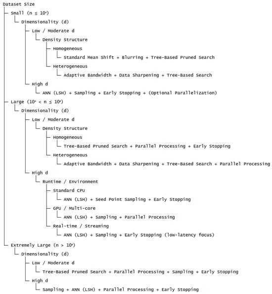
Figure 3.
Decision framework for selecting acceleration strategies based on dataset characteristics and computational constraints.
4. Conclusions
Mean Shift remains a powerful and conceptually elegant non-parametric clustering technique, but its widespread adoption has been historically constrained by high computational costs. This paper provided a comprehensive examination of optimization strategies for accelerating Mean Shift, encompassing parallelization, trajectory reduction, neighborhood pruning, adaptive bandwidth selection, and kernel approximation techniques. By systematically analyzing their theoretical underpinnings, computational complexity, accuracy characteristics, and combinability, we offered a structured framework for understanding and applying these methods in practice.
The main contribution and novelty of this work lie in the systematization and generalization of diverse strategies for accelerating the Mean Shift algorithm. A large number of original research papers, each containing experimental evaluation results on individual acceleration methods, were carefully systematized and summarized to support this study. The goal was to provide a high-level theoretical generalization of the extensive body of experimental findings reported in the literature and to integrate them into a coherent analytical framework.
A deep and systematic theoretical analysis was conducted to rigorously assess and compare the positive impact of each acceleration strategy on reducing the computational complexity of the general Mean Shift algorithm. This analysis focuses on deriving and formalizing the asymptotic behavior of different approaches, examining their scalability, accuracy characteristics, and interaction patterns. A pairwise compatibility matrix was introduced to characterize synergistic and conflicting interactions among strategies, thereby clarifying how multiple methods can be effectively combined. Building upon this analysis, the study introduces a key novel element—a practical decision framework for selecting suitable acceleration strategies based on dataset characteristics and computational constraints. Together with the developed taxonomy, combinability analysis, and scenario-based recommendations, this framework establishes a systematic and theoretically grounded foundation for understanding, evaluating, and applying Fast Mean Shift methods, effectively bridging the gap between a large, fragmented experimental literature and a unified, high-level theoretical perspective.
Our study highlighted that no single acceleration technique universally dominates across all scenarios. Instead, the effectiveness of each strategy depends critically on dataset characteristics such as size, dimensionality, and density structure, as well as the available computational resources. Parallel processing provides near-linear speedups with minimal algorithmic changes, while trajectory reduction methods such as seed sampling and early stopping yield substantial runtime reductions without compromising clustering quality. Neighborhood search acceleration via tree-based or approximate methods effectively addresses the quadratic kernel evaluation bottleneck, and kernel approximation techniques like the Fast Gauss Transform offer additional gains in low-dimensional regimes. Importantly, many of these strategies are complementary, enabling synergistic combinations tailored to specific application settings.
To support practical deployment, we proposed a structured mapping between optimization methods and algorithmic pipeline stages, as well as scenario-based recommendations for selecting appropriate combinations. This systematic perspective bridges methodological developments with real-world implementation considerations, helping practitioners navigate the trade-offs between accuracy and computational efficiency.
Future work may extend this framework in several directions. Promising avenues include adaptive hybrid strategies that dynamically select acceleration techniques based on data characteristics during runtime, integration with streaming and online clustering settings, and leveraging emerging hardware such as tensor cores and specialized accelerators for further gains. Additionally, combining Fast Mean Shift techniques with modern deep learning pipelines offers a compelling direction for large-scale, high-dimensional data analysis.
The strategies and guidelines presented in this paper provide both a theoretical foundation and a practical roadmap for making Mean Shift clustering tractable and efficient in contemporary large-scale analytical environments.
Author Contributions
Conceptualization, R.M.; methodology, R.M.; software, R.M.; validation, A.K.; formal analysis, M.A.; investigation, R.M.; resources, R.M. and A.K.; data curation, M.A.; writing—original draft preparation, R.M.; writing—review and editing, R.M., A.K., and M.A.; visualization, R.M.; supervision, R.M.; project administration, A.K.; funding acquisition, A.K. All authors have read and agreed to the published version of the manuscript.
Funding
This research was funded by the Science Committee of the Ministry of Science and Higher Education of the Republic of Kazakhstan (grant no. AP23486904).
Data Availability Statement
No new data were created or analyzed in this study. Data sharing is not applicable to this article.
Conflicts of Interest
The authors declare no conflicts of interest.
Abbreviations
The following abbreviations are used in this manuscript:
| MS | Mean Shift |
| Probability Density Function | |
| KDE | Kernel Density Estimation |
| BW | Bandwidth (in kernel functions) |
| kNN | k-Nearest Neighbor |
| k-d Tree | k-dimensional Tree |
| ANN | Approximate Nearest Neighbors |
| LSH | Locality-Sensitive Hashing |
| BMS | Blurring Mean Shift |
| FGT | Fast Gauss Transform |
| DBSCAN | Density-Based Spatial Clustering of Applications with Noise |
| GMM | Gaussian Mixture Model |
| CPU | Central Processing Unit |
| GPU | Graphics Processing Unit |
References
- Fukunaga, K.; Hostetler, L. The estimation of the gradient of a density function, with applications in pattern recognition. IEEE Trans. Inf. Theory 1975, 21, 32–40. [Google Scholar] [CrossRef]
- Georgescu, B.; Shimshoni, I.; Meer, P. Mean shift based clustering in high dimensions: A texture classification example. In Proceedings of the Ninth IEEE International Conference on Computer Vision, Nice, France, 13–16 October 2003; IEEE: Piscataway, NJ, USA, 2003; pp. 456–463. [Google Scholar]
- Cheng, Y. Mean shift, mode seeking, and clustering. IEEE Trans. Pattern Anal. Mach. Intell. 1995, 17, 790–799. [Google Scholar] [CrossRef]
- Akhmetov, I.; Mladenovic, N.; Mussabayev, R. Using K-Means and Variable Neighborhood Search for Automatic Summarization of Scientific Articles. In Variable Neighborhood Search; Lecture Notes in Computer Science; Springer: Cham, Switzerland, 2021; pp. 166–175. [Google Scholar] [CrossRef]
- Mussabayev, R.; Mladenovic, N.; Jarboui, B.; Mussabayev, R. How to Use K-means for Big Data Clustering? Pattern Recognit. 2023, 137, 109269. [Google Scholar] [CrossRef]
- Zhao, M.; Jha, A.; Liu, Q.; Millis, B.A.; Mahadevan-Jansen, A.; Lu, L.; Landman, B.A.; Tyska, M.J.; Huo, Y. Faster Mean-shift: GPU-accelerated clustering for cosine embedding-based cell segmentation and tracking. Med. Image Anal. 2021, 71, 102048. [Google Scholar] [CrossRef]
- Wu, K.L.; Yang, M.S. Mean shift-based clustering. Pattern Recognit. 2007, 40, 3035–3052. [Google Scholar] [CrossRef]
- Kim, J.; Lee, S.; Lee, G.; Park, Y.; Hong, Y. Using a Method Based on a Modified K-Means Clustering and Mean Shift Segmentation to Reduce File Sizes and Detect Brain Tumors from Magnetic Resonance (MRI) Images. Wirel. Pers. Commun. 2016, 89, 993–1008. [Google Scholar] [CrossRef]
- Jabar, F.H.A.; Ismail, W.; Salam, R.A.; Hassan, R. Image segmentation using a hybrid clustering technique and mean shift for automated detection acute leukaemia blood cells images. J. Theor. Appl. Inf. Technol. 2015, 76, 88–96. [Google Scholar]
- Shen, J.; Zhou, W.; Liu, N.; Sun, H.; Li, D.; Zhang, Y. An Anchor-Free Lightweight Deep Convolutional Network for Vehicle Detection in Aerial Images. IEEE Trans. Intell. Transp. Syst. 2022, 23, 24330–24342. [Google Scholar] [CrossRef]
- Ramakrishnan, V.; Chenniappan, P.; Dhanaraj, R.K.; Hsu, C.H.; Xiao, Y.; Al-Turjman, F. Bootstrap aggregative mean shift clustering for big data anti-pattern detection analytics in 5G/6G communication networks. Comput. Electr. Eng. 2021, 95, 107380. [Google Scholar] [CrossRef]
- Comaniciu, D.; Meer, P. Mean shift: A robust approach toward feature space analysis. IEEE Trans. Pattern Anal. Mach. Intell. 2002, 24, 603–619. [Google Scholar] [CrossRef]
- Chang-Chien, S.J.; Hung, W.L.; Yang, M.S. On mean shift-based clustering for circular data. Soft Comput. 2012, 16, 1043–1060. [Google Scholar] [CrossRef]
- Nguyen, H.T.; Tran, T.B.; Luong, H.H.; Le, T.P.; Tran, N.C. Improving disease prediction using shallow convolutional neural networks on metagenomic data visualizations based on mean-shift clustering algorithm. Int. J. Adv. Comput. Sci. Appl. 2020, 11, 52–60. [Google Scholar] [CrossRef]
- Becker, D.G.; Braun, W.J.; White, B.J.G. Interval-censored unimodal kernel density estimation via data sharpening. J. Stat. Comput. Simul. 2017, 87, 2023–2037. [Google Scholar] [CrossRef]
- Senoussaoui, M.; Kenny, P.; Dumouchel, P.; Stafylakis, T. Efficient iterative mean shift based cosine dissimilarity for multi-recording speaker clustering. In Proceedings of the 2013 IEEE International Conference on Acoustics, Speech and Signal Processing, Vancouver, BC, Canada, 26–31 May 2013; pp. 7712–7715. [Google Scholar] [CrossRef]
- Jain, A.; Nandakumar, K.; Ross, A. Score normalization in multimodal biometric systems. Pattern Recognit. 2005, 38, 2270–2285. [Google Scholar] [CrossRef]
- Alam, M.J.; Ouellet, P.; Kenny, P.; O’Shaughnessy, D. Comparative evaluation of feature normalization techniques for speaker verification. In Proceedings of the International Conference on Nonlinear Speech Processing, Las Palmas de Gran Canaria, Spain, 7–9 November 2011; Springer: Berlin/Heidelberg, Germany, 2011; pp. 246–253. [Google Scholar]
- Aksoy, S.; Haralick, R.M. Feature normalization and likelihood-based similarity measures for image retrieval. Pattern Recognit. Lett. 2001, 22, 563–582. [Google Scholar] [CrossRef]
- Du, R.; Wu, Q.; He, X.; Yang, J. MIL-SKDE: Multiple-instance learning with supervised kernel density estimation. Signal Process. 2013, 93, 1471–1484. [Google Scholar] [CrossRef]
- Schubert, E.; Sander, J.; Ester, M.; Kriegel, H.P.; Xu, X. DBSCAN revisited, revisited: Why and how you should (still) use DBSCAN. ACM Trans. Database Syst. 2017, 42, 1–21. [Google Scholar] [CrossRef]
- Mussabayev, R. Optimizing Euclidean Distance Computation. Mathematics 2024, 12, 3787. [Google Scholar] [CrossRef]
- Tehreem, A.; Khawaja, S.G.; Khan, A.M.; Akram, M.U.; Khan, S.A. Multiprocessor architecture for real-time applications using mean shift clustering. J. Real-Time Image Process. 2019, 16, 2233–2246. [Google Scholar] [CrossRef]
- Cho, H.; Kang, S.J.; Cho, S.I.; Kim, Y.H. Image Segmentation Using Linked Mean-Shift Vectors and Its Implementation on GPU. IEEE Trans. Consum. Electron. 2014, 60, 719–727. [Google Scholar] [CrossRef]
- Beck, G.; Duong, T.; Lebbah, M.; Azzag, H.; Cérin, C. A distributed approximate nearest neighbors algorithm for efficient large scale mean shift clustering. J. Parallel Distrib. Comput. 2019, 134, 128–139. [Google Scholar] [CrossRef]
- Kalimoldayev, M.N.; Siladi, V.; Satymbekov, M.N.; Naizabayeva, L. Solving mean-shift clustering using MapReduce Hadoop. In Proceedings of the 2017 IEEE 14th International Scientific Conference on Informatics, Poprad, Slovakia, 14–16 November 2017; pp. 164–167. [Google Scholar] [CrossRef]
- You, L.; Jiang, H.; Chang, C.H.; Chen, L.; Cui, X.; Zhao, M.; Hu, J. GPU-accelerated Faster Mean Shift with euclidean distance metrics. In Proceedings of the 2022 IEEE 46th Annual IEEE Computers, Software, and Applications Conference (COMPSAC 2022), Los Alamitos, CA, USA, 27 June–1 July 2022; Leong, H., Sarvestani, S., Teranishi, Y., Cuzzocrea, A., Kashiwazaki, H., Towey, D., Yang, J., Shahriar, H., Eds.; IEEE: Piscataway, NJ, USA, 2022; pp. 211–216. [Google Scholar] [CrossRef]
- Huang, F.; Chen, Y.; Li, L.; Zhou, J.; Tao, J.; Tan, X.; Fan, G. Implementation of the parallel mean shift-based image segmentation algorithm on a GPU cluster. Int. J. Digit. Earth 2019, 12, 328–353. [Google Scholar] [CrossRef]
- Yuan, X.; Li, S.Z. Stochastic gradient kernel density mode-seeking. In Proceedings of the 2009 IEEE Conference on Computer Vision and Pattern Recognition, Miami, FL, USA, 20–25 June 2009; pp. 1926–1931. [Google Scholar] [CrossRef]
- Huimin, G.; Guo, P.; Lu, H. A fast mean shift procedure with new iteration strategy and re-sampling. In Proceedings of the 2006 IEEE International Conference on Systems, Man and Cybernetics, Taipei, Taiwan, 8–11 October 2006; Volume 3, pp. 2385–2389. [Google Scholar] [CrossRef]
- Leung, A.P.; Gong, S. Mean-shift tracking with random sampling. In Proceedings of the British Machine Vision Conference 2006, Edinburgh, UK, 4–7 September 2006; Volume 2, pp. 729–738. [Google Scholar]
- Nieto, M.; Cuevas, C.; Salgado, L.J.; García, N.N. Line segment detection using weighted mean shift procedures on a 2D slice sampling strategy. Pattern Anal. Appl. 2011, 14, 149–163. [Google Scholar] [CrossRef]
- Kilic, V.; Barnard, M.; Wang, W.; Hilton, A.D.; Kittler, J.V. Mean-Shift and Sparse Sampling-Based SMC-PHD Filtering for Audio Informed Visual Speaker Tracking. IEEE Trans. Multimed. 2016, 18, 2417–2431. [Google Scholar] [CrossRef]
- Carreira-Perpinan, M.A. Fast nonparametric clustering with Gaussian blurring mean-shift. In Proceedings of the 23rd International Conference on Machine Learning, Pittsburgh, PA, USA, 25–29 June 2006; Association for Computing Machinery: New York, NY, USA, 2006; Volume 148, pp. 153–160. [Google Scholar] [CrossRef]
- Šurkala, M.; Mozdřeň, K.; Fusek, R.; Sojka, E. Hierarchical Blurring Mean-shift. In Advanced Concepts for Intelligent Vision Systems. ACIVS 2011; Lecture Notes in Computer Science; Springer: Ghent, Belgium, 2011; pp. 228–238. [Google Scholar] [CrossRef]
- Wang, W.; Carreira-Perpinan, M.A. Manifold blurring mean shift algorithms for manifold denoising. In Proceedings of the 2010 IEEE Computer Society Conference on Computer Vision and Pattern Recognition, San Francisco, CA, USA, 13–18 June 2010; pp. 1759–1766. [Google Scholar] [CrossRef]
- Grillenzoni, C. Design of Blurring Mean-Shift Algorithms for Data Classification. J. Classif. 2016, 33, 262–281. [Google Scholar] [CrossRef]
- Chen, T.L. On the convergence and consistency of the blurring mean-shift process. Ann. Inst. Stat. Math. 2015, 67, 157–176. [Google Scholar] [CrossRef][Green Version]
- Choi, E.; Hall, P. Data sharpening as a prelude to density estimation. Biometrika 1999, 86, 941–947. [Google Scholar] [CrossRef]
- Bentley, J.L. Multidimensional Binary Search Trees Used for Associative Searching. Commun. ACM 1975, 18, 509–517. [Google Scholar] [CrossRef]
- Omohundro, S.M. Five Balltree Construction Algorithms. 1989. Available online: https://api.semanticscholar.org/CorpusID:61067117 (accessed on 20 October 2025).
- Xiao, C.; Liu, M. Efficient mean-shift clustering using Gaussian KD-tree. Comput. Graph. Forum 2010, 29, 2065–2073. [Google Scholar] [CrossRef]
- Huang, W.; Zhang, J.; Yang, Y. A storage-efficient LSH scheme for high-dimensional ANN search. Pattern Recognit. 2025, 168, 111805. [Google Scholar] [CrossRef]
- Cui, Y.; Cao, K.; Zheng, G.; Zhang, F. An adaptive mean shift algorithm based on LSH. Procedia Eng. 2011, 23, 265–269. [Google Scholar] [CrossRef][Green Version]
- Zhang, X.; Cui, Y.; Li, D.; Liu, X.; Zhang, F. An adaptive mean shift clustering algorithm based on locality-sensitive hashing. OPTIK 2012, 123, 1891–1894. [Google Scholar] [CrossRef]
- Ren, Y.; Domeniconi, C.; Zhang, G.; Yu, G. A weighted adaptive mean shift clustering algorithm. In Proceedings of the 2014 SIAM International Conference on Data Mining, Philadelphia, PA, USA, 24–26 April 2014; Society for Industrial and Applied Mathematics: Philadelphia, PA, USA, 2014; Volume 2, pp. 794–802. [Google Scholar] [CrossRef]
- Jiang, Z.L.; Li, S.F.; Jia, X.P.; Zhu, H.L. An improved mean shift tracking method based on nonparametric clustering and adaptive bandwidth. In Proceedings of the 2008 International Conference on Machine Learning and Cybernetics, Kunming, China, 12–15 July 2008; Volume 5, pp. 2779–2784. [Google Scholar] [CrossRef]
- Meng, F.; Liu, H.; Liang, Y.; Wei, L.; Pei, J. A bidirectional adaptive bandwidth mean shift strategy for clustering. In Proceedings of the 2017 IEEE International Conference on Image Processing (ICIP), Beijing, China, 17–20 September 2017; Volume 2017, pp. 2448–2452. [Google Scholar] [CrossRef]
- Han, M.; Wang, J.; Wang, J.; Meng, J.; Cheng, Y. Research on target tracking algorithm based on mean shift with adaptive bandwidth. J. Comput. Methods Sci. Eng. 2022, 22, 661–675. [Google Scholar] [CrossRef]
- Yang, C.; Duraiswami, R.; Gumerov, N.A.; Davis, L. Improved fast gauss transform and efficient kernel density estimation. In Proceedings of the Ninth IEEE International Conference on Computer Vision, Nice, France, 13–16 October 2003; Volume 1, pp. 464–471. [Google Scholar]
- Elgammal, A.M.; Duraiswami, R.; Davis, L.S. Efficient kernel density estimation using the fast Gauss transform with applications to color modeling and tracking. IEEE Trans. Pattern Anal. Mach. Intell. 2003, 25, 1499–1504. [Google Scholar] [CrossRef]
- Lee, D.; Gray, A.G.; Moore, A.W. Dual-tree fast Gauss transforms. Adv. Neural Inf. Process. Syst. 2005, 18, 747–754. [Google Scholar]
- Mittelman, R.; Miller, E.L. Nonlinear filtering using a new proposal distribution and the improved fast Gauss transform with tighter performance bounds. IEEE Trans. Signal Process. 2008, 56, 5746–5757. [Google Scholar] [CrossRef][Green Version]
- Ren, Y.; Kamath, U.; Domeniconi, C.; Zhang, G. Boosted mean shift clustering. In Machine Learning and Knowledge Discovery in Databases. ECML PKDD 2014; Lecture Notes in Computer Science; Springer: Berlin/Heidelberg, Germany, 2014; pp. 646–661. [Google Scholar] [CrossRef]
- Yuan, X.T.; Hu, B.G.; He, R. Agglomerative mean-shift clustering. IEEE Trans. Knowl. Data Eng. 2012, 24, 209–219. [Google Scholar] [CrossRef]


Disclaimer/Publisher’s Note: The statements, opinions and data contained in all publications are solely those of the individual author(s) and contributor(s) and not of MDPI and/or the editor(s). MDPI and/or the editor(s) disclaim responsibility for any injury to people or property resulting from any ideas, methods, instructions or products referred to in the content. |
© 2025 by the authors. Licensee MDPI, Basel, Switzerland. This article is an open access article distributed under the terms and conditions of the Creative Commons Attribution (CC BY) license (https://creativecommons.org/licenses/by/4.0/).