Abstract
Background/Objectives: In computer graphics, virtual worlds are constructed and visualized through algorithmic processes. These environments are typically populated with objects defined by mathematical models, traditionally based on Euclidean geometry. However, there is increasing interest in exploring non-Euclidean geometries, which require adaptations of the modeling techniques used in Euclidean spaces. Methods: This paper focuses on defining parametric curves and surfaces within elliptic and hyperbolic geometries. We explore free-form splines interpreted as hierarchical motions along geodesics. Translation, rotation, and ruling are managed through supplementary curves to generate surfaces. We also discuss how to compute normal vectors, which are essential for animation and lighting. The rendering approach we adopt aligns with physical principles, assuming that light follows geodesic paths. Results: We extend the Kochanek–Bartels spline to both elliptic and hyperbolic geometries using a sequence of geodesic-based interpolations. Simple recursive formulas are introduced for derivative calculations. With well-defined translation and rotation in these curved spaces, we demonstrate the creation of ruled, extruded, and rotational surfaces. These results are showcased through a virtual reality application designed to navigate and visualize non-Euclidean spaces.
Keywords:
splines; parametric curves and surfaces; hyperbolic geometry; elliptic geometry; transformations MSC:
51M09; 53A05; 65D17; 68U07
1. Introduction
Modeling in computer graphics constructs virtual worlds by defining object surfaces through mathematical equations. Two common approaches are implicit and parametric formulations. Implicit equations of the form describe the conditions a point must satisfy to lie on a surface, often involving constraints such as the distance, angle, or orthogonality. Implicit forms are particularly useful in ray tracing: by substituting the ray’s parametric equation into the surface equation, one obtains a scalar equation for the ray parameter.
Parametric modeling, in contrast, describes motion or shape directly. A parametric curve assigns a position to each parameter t, while a parametric surface extends this idea to two dimensions, generated by sweeping or interpolating curves. Many widely used graphics tools rely on such parametric constructions, with surfaces defined through extrusion, rotation, ruling, or interpolation of control points.
While Euclidean geometry underlies most existing modeling techniques, many applications benefit from extending them to non-Euclidean geometries. A common but limited strategy is to first design models in Euclidean space, tessellate the surfaces to small triangles, and then project vertices of the triangles into the curved space using central or stereographic projection, or with the exponential map [1]. However, because Euclidean and curved spaces differ in Gaussian curvature, any projection inevitably distorts either distances or angles, often breaking the modeler’s spatial intuition. A more natural approach is to define models directly within the target non-Euclidean geometry (Figure 1).
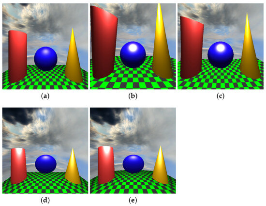
Figure 1.
Modeling the scene directly in curved spaces versus porting the scene from Euclidean geometry with the exponential map. The exponential map makes those points of Euclidean and non-Euclidean spaces correspond to each other that are at the same direction and the same distance from the geometry origin of the spaces. Note that the base rectangle is supposed to be bounded by lines, but they are made curved by porting, whereas in our direct modeling approach, they are correctly represented as geodesics of the space. (a) Euclidean reference. (b) Modeled in elliptic space. (c) Ported to elliptic space. (d) Modeled in hyperbolic space. (e) Ported to hyperbolic space.
1.1. Previous Work
Curves can be specified by their parametric equation or by interpolation or approximation of control points. In Euclidean space, this is based on the center of mass analogy. Every control point gets parameter dependent mass , and the point of the curve associated with the given parameter t is the center of mass of the resulting mechanical system:
Unfortunately, this does not work in curved spaces, where, even if the control points are in the space of the geometry, their linear combination may be out.
There are several ways to generalize parametric spline curves to non-Euclidean spaces—see the recent survey of Mancinelli and Puppo [2]. The center of mass can be given another interpretation [3,4] as the point from which the sum of the weighted squared distances to the control points is minimal:
where is the distance of points and , and the search is constrained to the space of the geometry. In non-Euclidean geometry, finding this optimum requires numerical optimization, which complicates the application of automatic differentiation techniques. The same is true for alternative generalizations of spline curves in terms of functional minimization [5,6,7,8] or recursive subdivision [9,10]. Yet, efficient and accurate derivatives are crucial for shading, animation, and differentiable rendering.
As non-Euclidean geometries also incorporate the concept of lines as geodesic curves [11], spline evaluation can be made geometry-independent if its construction is traced back to a sequence of interpolations along geodesics. Famous examples of parametric curve definition based on linear interpolations are the de Casteljau construction of the Bézier curve [12], the de Boor construction of the B-spline [13], the Neville’s algorithm for Lagrange polynomial interpolation, or the Barry–Goldman method [14] for evaluating Catmull–Rom splines [15]—see the monograph [16] for a unified treatment based on the concept of blossoming [17].
The earliest attempts at extending linear interpolation to curved spaces focused on curves in two- or three-dimensional spheres (i.e., unit vectors or quaternions). Shoemake proposed including spherical linear interpolation (SLERP) [18] and spherical cubic interpolation (SQUAD) [19], which have become widely used in the field of computer animation and inspired many practical algorithms [20,21,22]—see ([23], Ch. 25) and [24] for overviews. The concept of blossoming has also been generalized to spherical geometry in various ways [25,26]. Schaefer and Goldman [27] have introduced variants of Bézier, Lagrange, and B-spline curves, as well as Catmull–Rom splines defined over spheres of arbitrary dimensions. Geier has proposed generalizations of Catmull–Rom and Kochanek–Bartels [28] splines to quaternions (as foundation for the Python 3.13 package splines 0.3.3 (https://pypi.org/project/splines/, accessed on 25 July 2025)).
The aforementioned parametric curve constructions are specific to spherical geometries. De Casteljau’s algorithm has also been successfully extended to general Riemannian manifolds [29,30,31,32,33,34]; however, the practical examples in these works are usually restricted to Lie groups, such as SO(3) or SE(3). We are aware of only a few publications that consider parametric curves in the hyperbolic plane [31,35] and none that do so in hyperbolic 3-space.
Rendering in curved spaces poses further challenges. Since light follows geodesics, visibility computations in ray tracing must generalize intersection tests to geodesic paths [36,37,38]. Object–space algorithms can be adapted by exploiting Klein’s model, which maps geodesics to straight lines while preserving the visibility order [39,40].
1.2. Contributions
The purpose of this paper is to extend efficient Euclidean modeling and rendering techniques to constant-curvature non-Euclidean spaces. Our contributions are as follows:
- A generalization of the Kochanek–Bartels spline (in special cases also known as the Overhauser or Catmull–Rom spline) to curved geometries, including elliptic and hyperbolic spaces. The resulting curve interpolates control points, offers local control, and is defined entirely through motions along geodesics. In contrast to Geier’s approach that provides a piecewise-Bézier formulation, our solution is based on the blending of quadratic interpolants.
- An extension of translational, rotational, and ruled parametric surfaces to curved spaces.
- Methods for computing spline tangents and surface normals in non-Euclidean geometries, supporting applications in shading, animation, and differentiable rendering.
The remainder of the paper is organized as follows. Section 1.3 reviews the embedding space model of Euclidean, elliptic, and hyperbolic geometries. In Section 2.1, we present our spline construction for curved spaces, while Section 2.2 focuses on the computation of tangent vectors. Section 2.4 derives formulas for pure translations and rotations, which are then applied in Section 2.5 to generate extruded, rotated and ruled parametric surfaces. Section 2.6 discusses efficient GPU-based rendering of these objects. The results are reported in Section 3, and the paper concludes with final remarks in Section 4.
1.3. The Embedding Space Model of Geometries and Notations
Euclidean, elliptic, and hyperbolic geometries can be described within a unified framework by embedding them into a higher-dimensional space [41,42]. Specifically, 3D geometries are realized as subsets of a 4D embedding space, where each point is represented by a vector with four coordinates (see Table 1 for notations). Figure 2 illustrates the simplified case of 2D geometries embedded in 3D space.

Table 1.
Notations used in this paper.
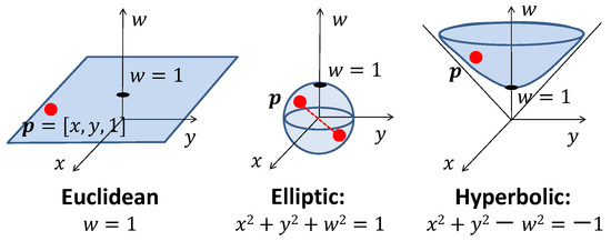
Figure 2.
Embedding of the 2D Euclidean, elliptic, and hyperbolic geometries into 3D space. Points of Euclidean geometry lie on the plane , points of elliptic geometry lie on the unit sphere , and points of hyperbolic geometry correspond to the upper sheet of the two-sheeted hyperboloid .
The metric in the embedding space is defined by the dot product . For Euclidean and elliptic geometries, this is the standard Euclidean dot product; however, hyperbolic geometry requires a Minkowski embedding with the Lorentzian dot product. To unify notation, we introduce the curvature sign , defined as
With this, the general dot product becomes
For Euclidean 3D vectors, we also use the conventional dot symbol:
The embedding space is equipped with four basis vectors , that are normalized and mutually orthogonal:
1.3.1. Points
Points of elliptic and hyperbolic geometries lie on their respective hyperspheres:
In elliptic geometry, antipodal points and are identical, i.e., a point corresponds to a diameter of the hypersphere. In hyperbolic geometry, only the upper sheet is considered, requiring .
The point of embedding coordinates lies in all three geometries (Euclidean, elliptic, hyperbolic). It is called the geometry origin and is denoted by .
1.3.2. Vectors
A vector based at a point must not point out of the space of the geometry. This requires to lie in the 3D tangent hyperplane of the hypersphere at :
1.3.3. Lines and Distances
Geodesics in elliptic and hyperbolic geometries arise from large circles that are intersections of the hypersphere with planes through the origin. Consider a sphere of radius R centered at the origin, a starting point , and an initial unit tangent vector . The parametric equation of the resulting great circle is given by
which can be interpreted as a unit speed motion, since .
From the equation of a general main circle, the line of the elliptic geometry can be obtained by considering a unit radius sphere ():
The distance d between points and is the travel time along the geodesic:
The absolute value operation is needed because a point can be represented by both and . To resolve this ambiguity, we require that for points of a single object, the scalar product must be positive. When the distance from the camera is needed by rendering, objects, where the dot product with the eye position is negative, are removed by clipping, but the scene is rendered two times, once with the original points and once with .
The geodesic segment between and at distance d can also be written as a spherical interpolation (SLERP) [18]:
which yields a uniform motion of speed d if is assumed to be the time.
In hyperbolic geometry, the geodesic takes the form
corresponding to a sphere of imaginary radius . The distance d between points and is
A geodesic segment can be expressed as a hyperbolic interpolation [43]:
Both spherical and hyperbolic interpolations work for as well, i.e., when . For small d values, they can be approximated by the Euclidean version:
2. Methods
This section introduces our approach for defining spline curves in curved spaces and generating surfaces through curve transformations. We employ a unified notation that simultaneously handles elliptic and hyperbolic geometries: functions and denote and in the elliptic case and and in the hyperbolic case.
The uniform interpolation between vectors and that are associated with points at distance d is defined as
The line segment with endpoints and is obtained by interpolating the location along their geodesic:
2.1. Geometry-Independent Interpolating Spline
We construct a smooth curve that interpolates a sequence of control points at knot values , respectively. Both the control points and the resulting curve lie in the underlying geometry:
The construction relies only on the constant-speed motion along the geodesic defined by at and at . Thus, by substituting the appropriate line equation, the same algorithm applies in Euclidean, elliptic, and hyperbolic geometries.
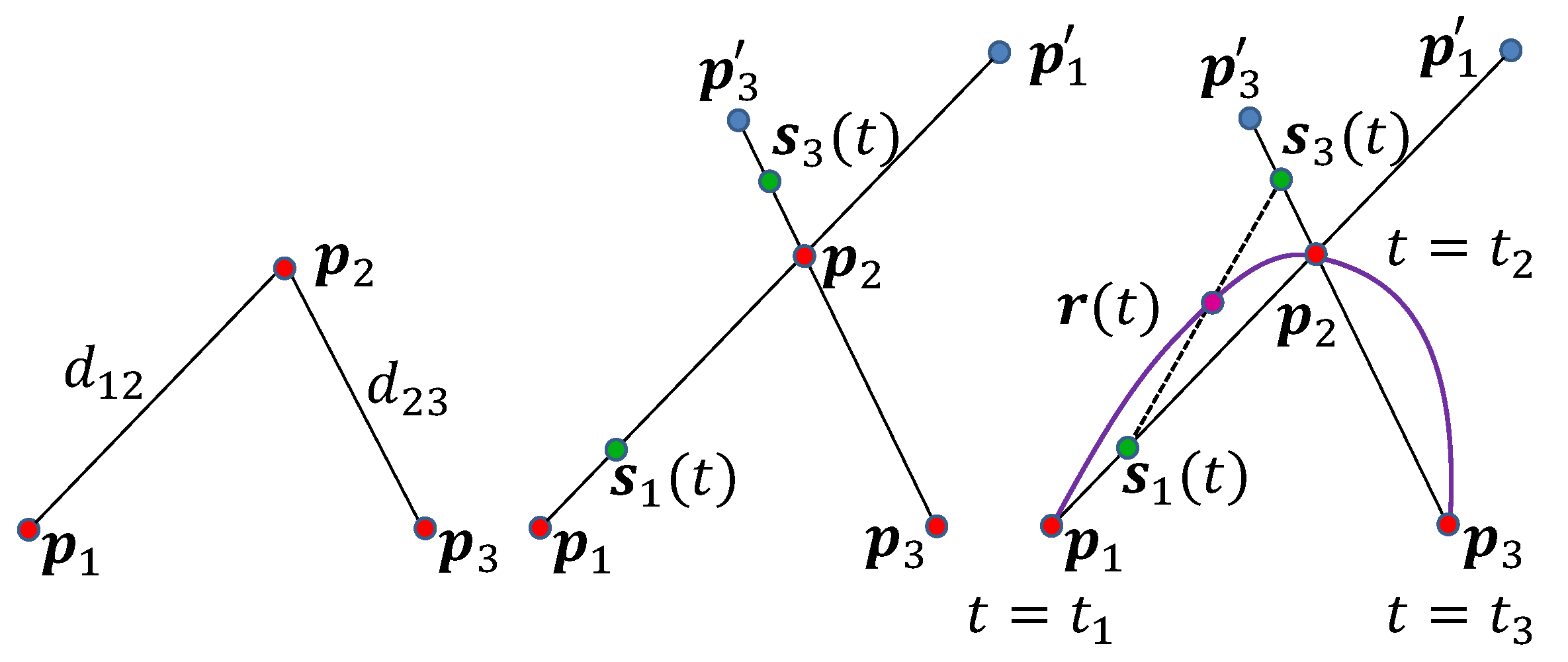
Consider three control points to be interpolated at (Figure 3). Let and denote the distances between and , respectively. We introduce two auxiliary points: on the extension of , located at distance from , and on the extension of , located at distance from .
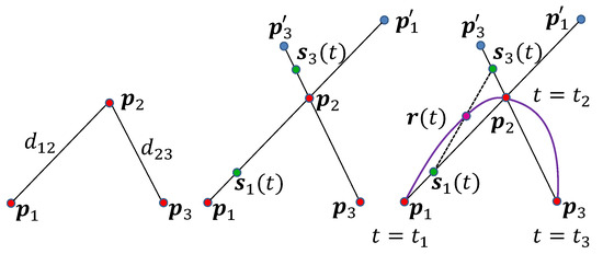
Figure 3.
Spline construction for three control points as a composition of three motions. Motion goes from to , motion goes from to , and the spline is a motion between and .
Define motions , extending toward , and , extending toward . Finally, let the spline of the three points be the motion interpolating between and :
Interpolation conditions are satisfied when
A convenient choice of the line parameters is
yielding auxiliary distances
Here, is the tension parameter, controlling the curvature near control points, while is the bias parameter, shifting the curve to anticipate or overshoot a turn.
For in Euclidean space, the parametrization reduces to
which yields Neville’s construction of the Lagrange interpolating curve:
As with classical Lagrange interpolation, this construction suffers from oscillations and poor local control for larger sets of control points.
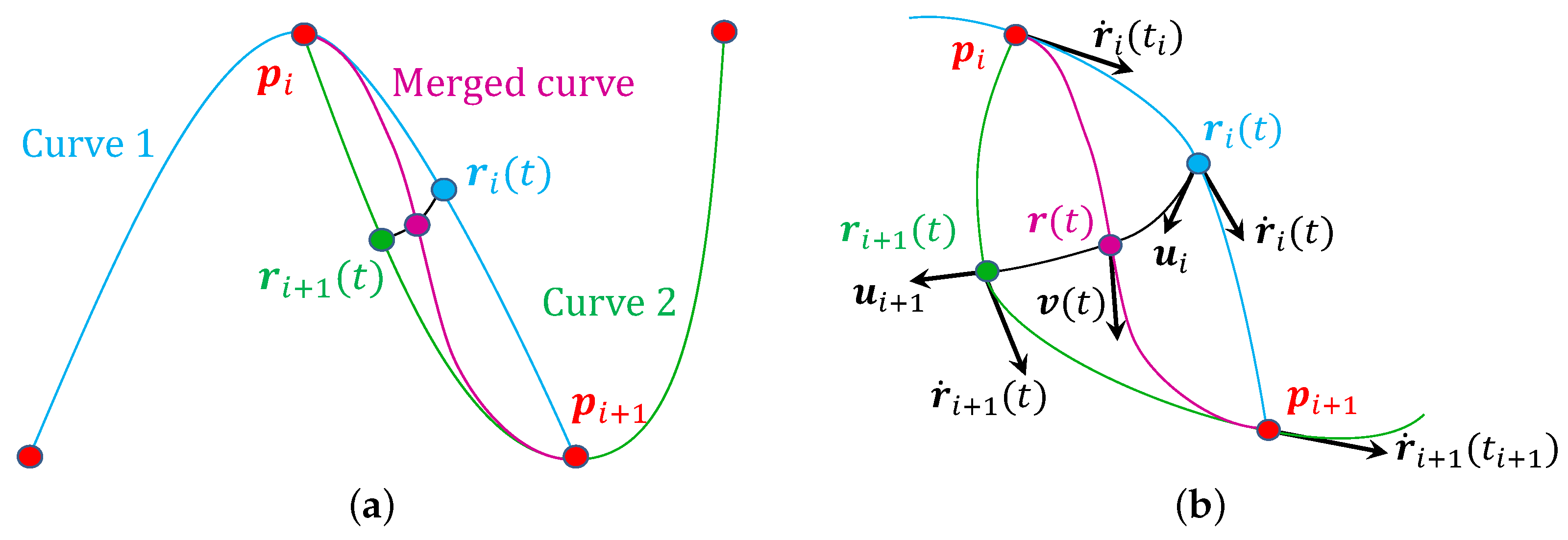
To address these issues, we adapt Overhauser’s approach [44]: the proposed interpolation scheme is applied only to local triplets, e.g., and then , etc. The final curve is obtained by merging the overlapping segments using geodesic blending (Figure 4a):
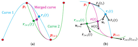
Figure 4.
Overhauser style blending of two spline segments and sharing two control points and . (a) Blending Curve 1 defined by and Curve 2 defined by . (b) Zoom in for continuity analysis. and are the velocities, and and are the unit tangents at the endpoints of the blending geodesic.
2.2. Spline Tangent Calculation
In applications such as path animation based on the Frenet frame or illumination computations involving surface normals, it is necessary to evaluate the tangent vector of the spline at specific points. This tangent is obtained as the derivative of the spline with respect to its parameter. Since our spline is constructed as a hierarchy of constant-speed motions along geodesics, we propose a recursive algorithm for tangent computation.
At each step, the inputs are the geodesic endpoints and and their velocities and (Figure 5). In addition, the distance d between the endpoints and the unit direction vectors and of the geodesic at the endpoints can be expressed as
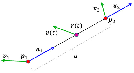
Figure 5.
One step of the derivative calculation. Inputs are endpoint positions , , endpoint velocities , , and the derived quantities including distance d and unit direction vectors and . Outputs are the position and velocity at time t.
The derivative of
yields the velocity at point on the geodesic. It consists of three terms: (i) the motion of the endpoints, (ii) the change ointhe interpolation parameter , and (iii) the variation in the geodesic length. The formula for the velocity is
where the derivative of the geodesic distance d between and is
The proof is given in Appendix A.
2.3. Continuity Analysis
In between the control points, the spline of Equation (14) is continuously differentiable by an arbitrary number of times. To examine the smoothness at the control points, let us take the derivative expressed by Equation (15) of the spline defined in Equation (14), where is the derivative of segment i at parameter point t, and is the derivative of segment (Figure 4b). To prove continuous differentiability, i.e., continuity, we need to show that the derivative of goes to the derivative of and the derivative of when t converges to and , respectively. As segment i and segment share control points and , the distance d between and converges to zero when t goes to or . Substituting these into Equation (15), we obtain
since and if , and if both and d are zero. Similarly, when t goes to , becomes 1 and d goes to zero; thus, we get
since and if , and if and . This means that the derivative of the merged spline at the control points depends just on that segment that has this control point in the middle of its three control points. Thus, the spline has continuous velocity, i.e., belongs to the class.
2.4. Transformations and Isometries
Our goal is to express transformations in non-Euclidean spaces in terms of explicit formulas, ideally as 4 × 4 matrix multiplications. Such transformations must map the geometry onto itself; that is, the image of any point must remain within the same space. Since isometries preserve the dot product, they also preserve membership in the geometry, as point belongs to the space precisely when . Thus, enforcing dot product preservation guarantees that transformed points remain valid. In practice, this condition is satisfied if the transformed basis vectors form an orthonormal frame, i.e., they satisfy Equations (2) and (3).
In Euclidean geometry, translations and rotations can be expressed as compositions of two planar reflections [40]. If the reflecting planes are parallel, the result is a translation; if they intersect, the result is a rotation around their line of intersection (Figure 6).
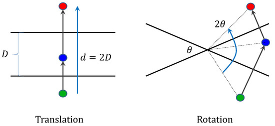
Figure 6.
Translation and rotation constructed from two planar reflections. If the planes are parallel and are at distance D, then the two reflections make a translation by distance . If the two planes are intersecting and have angle , then the two reflections are equivalent to a rotation by angle .
In elliptic and spherical geometries, parallels do not exist, and hence, true translations are absent. By contrast, in hyperbolic geometry there are many parallels, making the translation as reflections on parallels ambiguous. Nevertheless, both translations and rotations are essential for intuitive modeling. We therefore introduce the notions of pure rotation and pure translation. A pure rotation fixes the geometry origin, while a pure translation moves the origin to a new point. Moreover, translations must implement parallel transport, preserving direction as closely as possible.
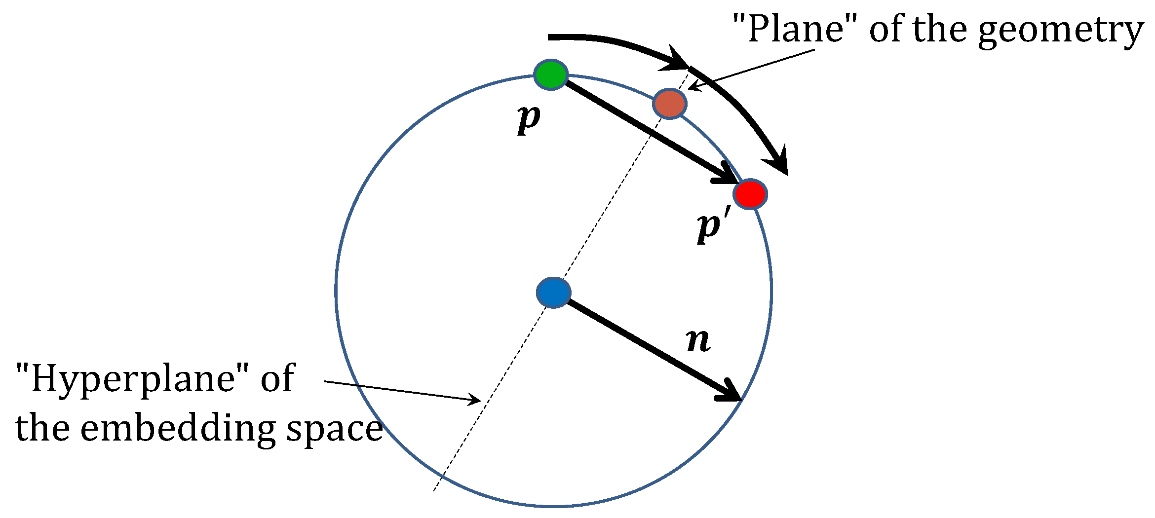
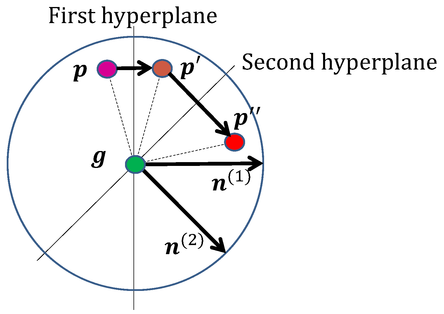
By spherical symmetry, reflection on a plane of the geometry corresponds to reflection on a hyperplane of the embedding space (Figure 7). Such a hyperplane must pass through the origin of the embedding space to map the curved space onto itself and can be written as
where is its normal.

Figure 7.
Reflection of on a plane of the geometry corresponds to a reflection on a hyperplane of normal in the embedding space (shown in a lower-dimensional example, where the plane is a point, and the hyperplane of the embedding space is a line).
Reflecting point across the hyperplane with normal yields
A second reflection, with normal , gives
Since depends linearly on , transformations defined by reflections can be implemented with 4 × 4 matrices.
2.4.1. Translation
To construct a pure translation, we compose two reflections so that the origin is mapped to (Figure 8). The first reflection plane passes through , and the second lies midway between and . To enforce parallel transport, the normals of both planes, together with and , must be coplanar. A convenient choice is
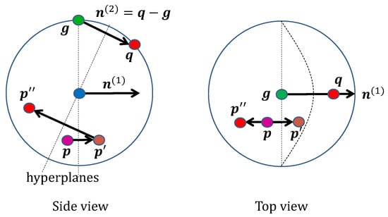
Figure 8.
Translation of to using two reflections, first on the hyperplane of normal to get and then on the hyperplane of normal to obtain . The first reflection does not affect geometry origin , but the second takes it to .
Substituting into Equation (19) yields the following closed-form expression for a pure translation (see Appendix B for proof):
2.4.2. Rotation
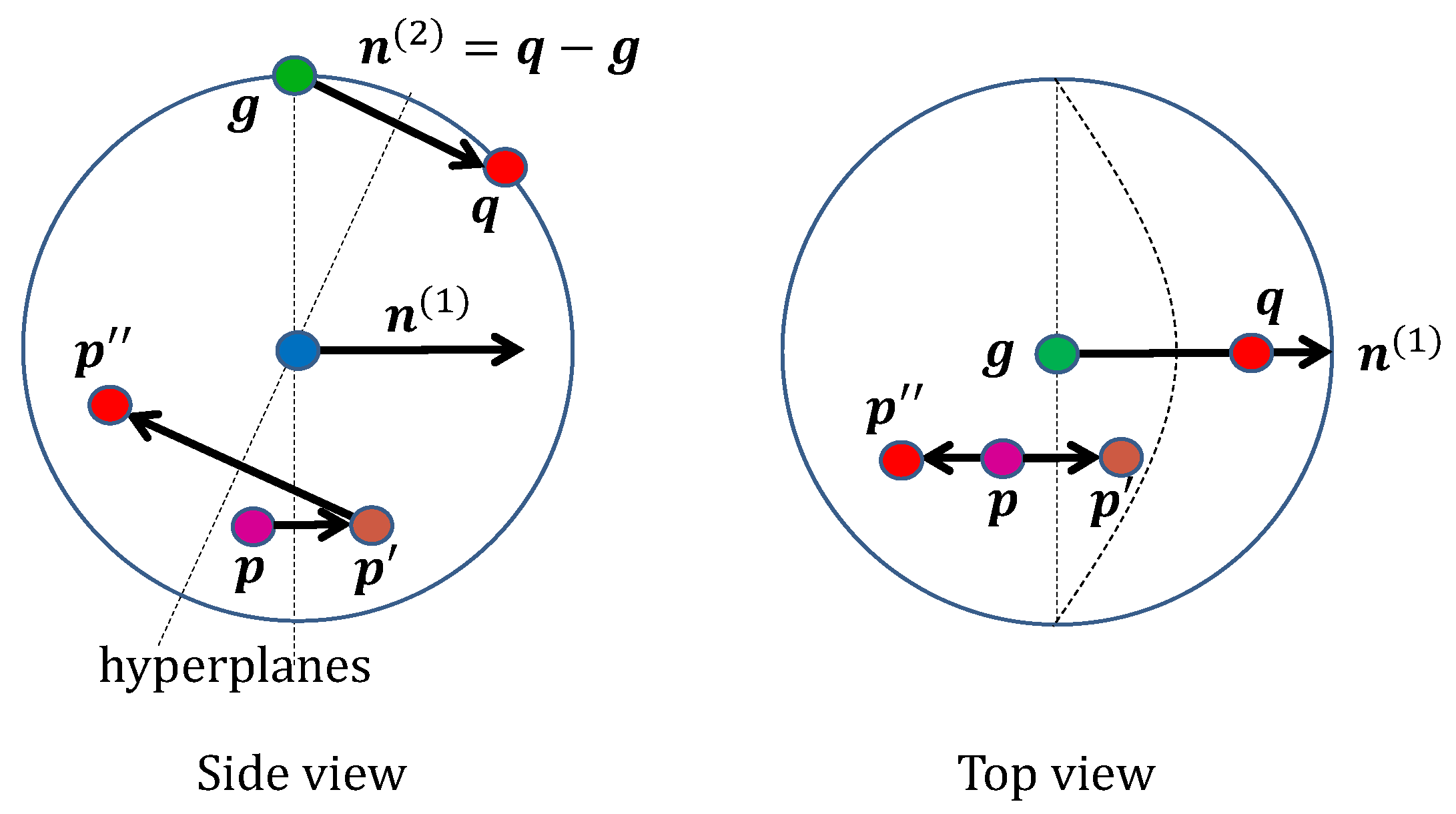
A pure rotation is also an isometry, but unlike a translation, it fixes the geometry origin (Figure 9). A reflection preserves the geometry origin if its w coordinate is zero; thus, we require . For simplicity, assume the normals have unit length. Then, Equation (19) reduces to
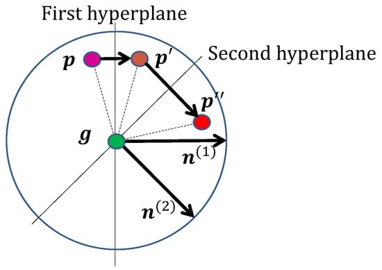
Figure 9.
Rotation constructed as a double reflection, first reflecting on the hyperplane of normal to get , and then reflecting on the hyperplane of normal to obtain (top view). As geometry origin is in both reflection hyperplanes, it is a fixed point of the transformation.
Here, the axis is given by
and the rotation angle is , where is the angle between the two normals.
Note that remains unchanged since the w coordinates of the normal vectors are zero, and the -coordinates follow Euclidean operations. Thus, in this setting the Rodrigues rotation formula applies not only in Euclidean space but also in hyperbolic and elliptic geometries.
2.5. Parametric Surfaces
Surfaces are two-dimensional manifolds, which means that two independent motions are required to define them. The first is a profile curve , describing the position of a point along the curve as a function of parameter u. The second is a transformation that moves the profile curve to sweep the surface. Two common transformations are translation (also called extrusion) and rotation. Alternatively, ruling generates a surface by prescribing two synchronized motions that define the endpoints of a moving line segment.
2.5.1. Extruded Surfaces
Translation is controlled by an additional spine curve parameterized by v, which translates the geometry origin to point . Substituting the current spine point into the target in Equation (21), the extruded surface point as a function of parameters u and v is given by
2.5.2. Rotational Surfaces
A rotational surface is generated by rotating the profile curve by an angle v around a unit-length axis passing through the geometry origin. Using Rodrigues’ formula, we obtain
2.5.3. Ruled Surfaces
A ruled surface is formed as the locus of points swept by a moving line segment. It is specified by two endpoint curves, and , defined as splines with common parameter u. Parameter then interpolates along the line segment, yielding
2.5.4. Tessellation
For rendering with the GPU pipeline, surfaces must be approximated by triangles. When triangles are sufficiently small, the curved patch can be approximately represented as the convex combination of its three vertices in the 4D embedding space. Approximating a parametric surface with a triangular mesh is called tessellation, which amounts to subdividing the parameter space into triangles. For each vertex of parameters , the parametric function provides the location in the 4D embedding space.
2.5.5. Surface Normals
Rendering requires the calculation of the reflected radiance of surfaces visible in pixels. Since the reflected radiance depends on the surface normal vector , tessellation must also address normal computation. The normal vector at must lie in the tangent space of the geometry to avoid pointing out of the manifold, i.e., must hold. Furthermore, must be orthogonal to the surface tangents and . Thus, the 4D normal is perpendicular to , , and , and can be expressed using the 4D analogue of the 3D cross product [45]:
2.6. Rendering
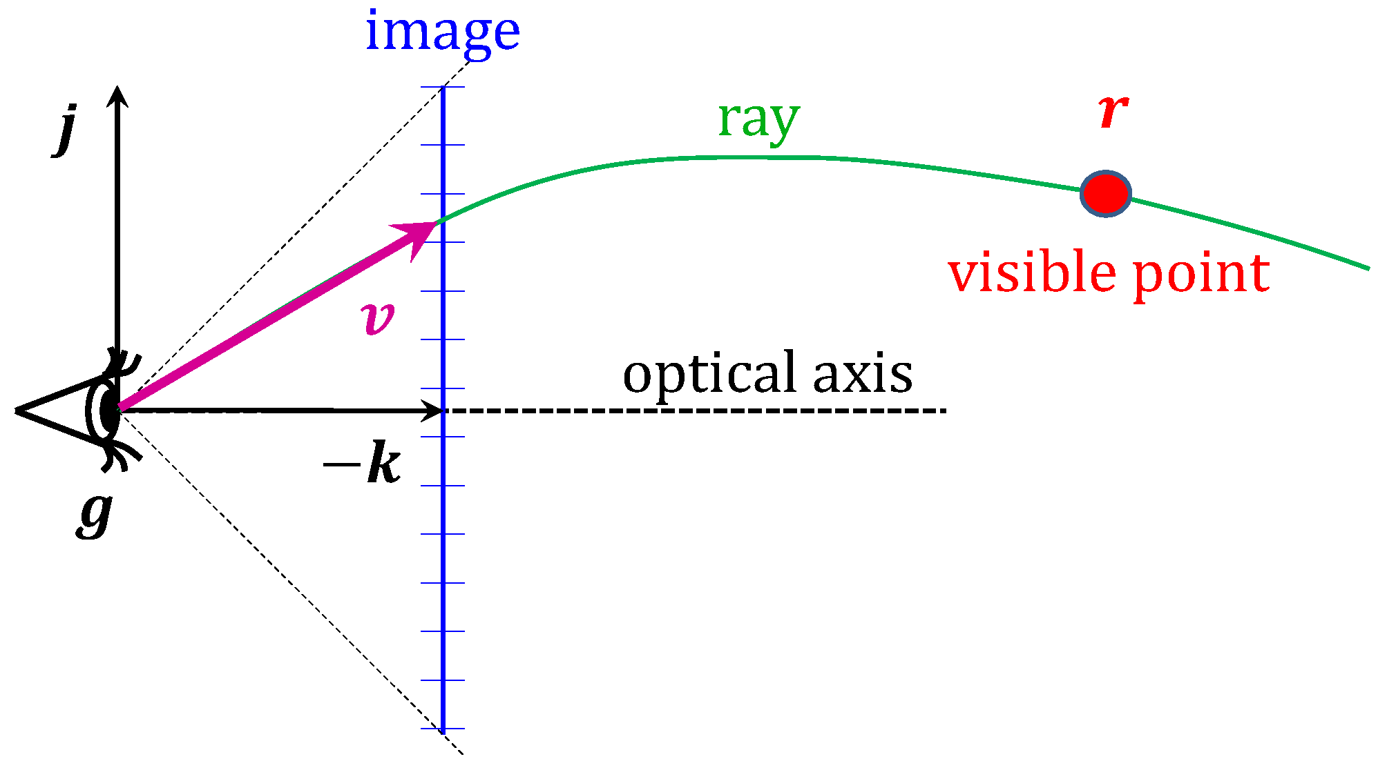
To generate an image of the virtual world, a camera must be introduced into the geometric space. Conceptually, a camera consists of an eye position , a set of pixels, and a rule that associates each pixel with the direction of a line containing points that are potentially visible through the pixel center. This construction follows from the fact that light travels along geodesics between the visible surfaces and the eye. The global orientation of the camera is specified by three orthogonal unit vectors in the tangent space of the eye position: the right direction , the up direction , and the negative view direction . Pixels are identified by Normalized Device Coordinates (NDC) , with the range boundaries corresponding to the edges of the image: is the bottom of the image, is the top, is the left boundary, and is the right boundary.
The mapping between directions and pixels simplifies considerably if the camera has canonical settings: the eye position is at the geometry origin , , , and . To achieve this, we apply an isometric transformation (translation and rotation) to both the scene and the camera. Because isometries act simultaneously on objects and the camera, the resulting image remains unchanged.
This transformation can be expressed as a multiplication with the following matrix [1]:
If the camera is small, we can rely on the analogy of Euclidean geometry (Figure 10). To associate pixel coordinates with ray direction , we set the x and y components of to the pixel NDCs scaled by factors and . The scaling should make sure that the z-component of the ray direction is equal to . With relative parameters and we can control the camera field-of-view and aspect ratio settings. Since the eye lies at the geometry origin, ray directions belong to its tangent space where :
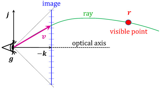
Figure 10.
Canonical camera setup: The eye is in geometry origin , the right direction is , the up direction is , and the viewing direction is , where the negative sign ensures that the frame is right-handed. The start of the ray is the eye. The current pixel determines the initial direction vector of the ray that contains the potentially visible points .
Using the geodesic equation, the visibility ray parameterized by distance d from the eye being in is
where is the normalized version of the ray direction. Taking into account that , the inverse operation is
If objects are defined implicitly by equations of the form
then their ray intersections can be determined by solving the scalar equation for d. Among all positive solutions across all objects, the smallest one determines the visible surface and thus the pixel color.
In object-space rendering, the focus is shifted from the pixels to object points, and the task is to determine the pixel in which object point appears. The unit direction of the ray containing is
where the distance d from the eye in satisfies
since .
The GPU expects the vertex shader to output points in homogeneous coordinates , where the pair equals the pixel’s normalized device coordinates, and is an increasing function of distance d, which is used for visibility determination. Thus, the point should be submitted in the following homogeneous form:
where we first applied Equation (28), then Equation (29), and finally Equation (30).
Setting W to , the homogeneous coordinates have the following form:
The clipping stage of the GPU retains points satisfying and . Inequality means that is positive, which requires to be positive. This is always the case in hyperbolic geometry, but in elliptic geometry, is positive only in half of the main circle. Objects that are closer in the opposite direction are clipped away. To resolve this problem, the scene is rendered two times in elliptic geometry: once with the original points , and once with negated points [39].
If W is positive, then inequalities are satisfied by the construction in Equation (32), since the NDCs are between and 1.
For coordinate , function should be set to get the points of the view frustum to pass the clipping test. Let us search Z as a linear function of and :
where parameters a and b are determined from the distance range of the view frustum. Using Equation (30) on the optical axis,
since on the optical axis ; thus, . Substituting this and Equation (31) into Equation (34), we get
On the optical axis, the visibility ray enters the visible frustum at and leaves it at . The entry point must be on the front clipping plane of equation , with the exit point on the back clipping plane of equation , which establishes a system of linear equations for unknowns a and b:
Solving this, the a and b parameters are
3. Results
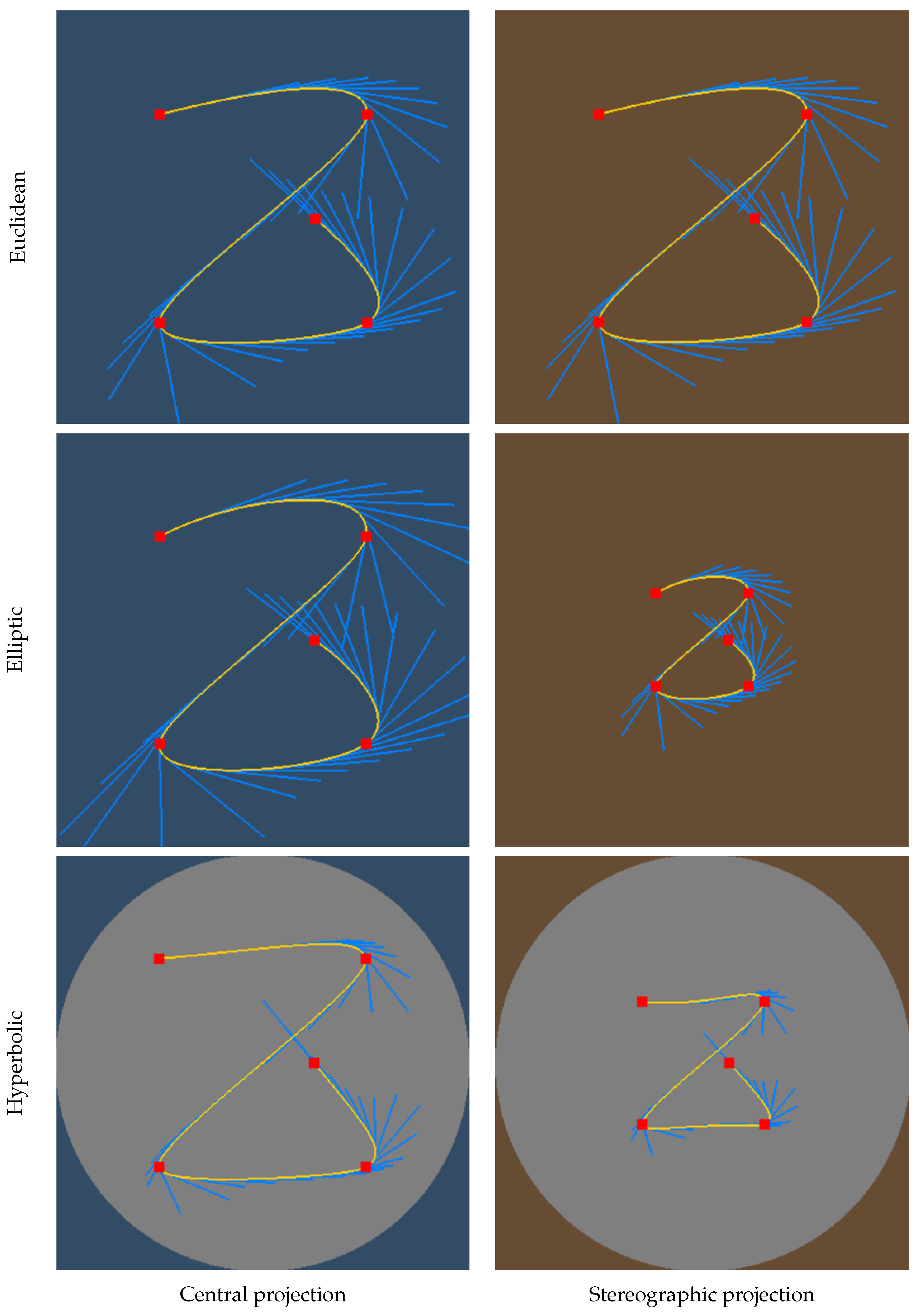
In order to demonstrate the discussed algorithms, first we compare the 2D spline curves in Euclidean, elliptic, and hyperbolic planes. To visualize the curved spaces, they are projected onto the Euclidean plane with central projection (Klein’s model) and stereographic projection (Poincaré’s model). In the case of hyperbolic geometry, the whole plane is projected to a circle that is drawn in gray. For elliptic and Euclidean geometries, the projection is infinitely large; so, only a part of the projected plane is visible here. The Klein model shows geodesics as Euclidean lines, while the Poincaré model preserves angles but presents geodesics as circular arcs. Figure 11 shows the proposed spline with unit bias and tension for all three considered geometries and for both central and stereographic projections. The tangents are also depicted to show the results of the derivative calculation.
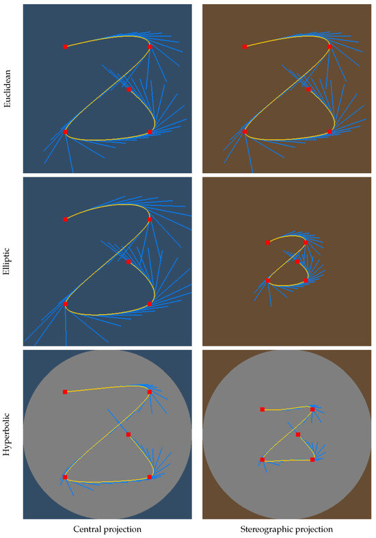
Figure 11.
Our spline with yellow color in Euclidean (top), elliptic (middle), and hyperbolic (bottom) geometries. Left: central projection (Klein’s model). Right: stereographic projection (Poincaré’s model). Cyan line segments indicate tangents. Red squares are the control points.
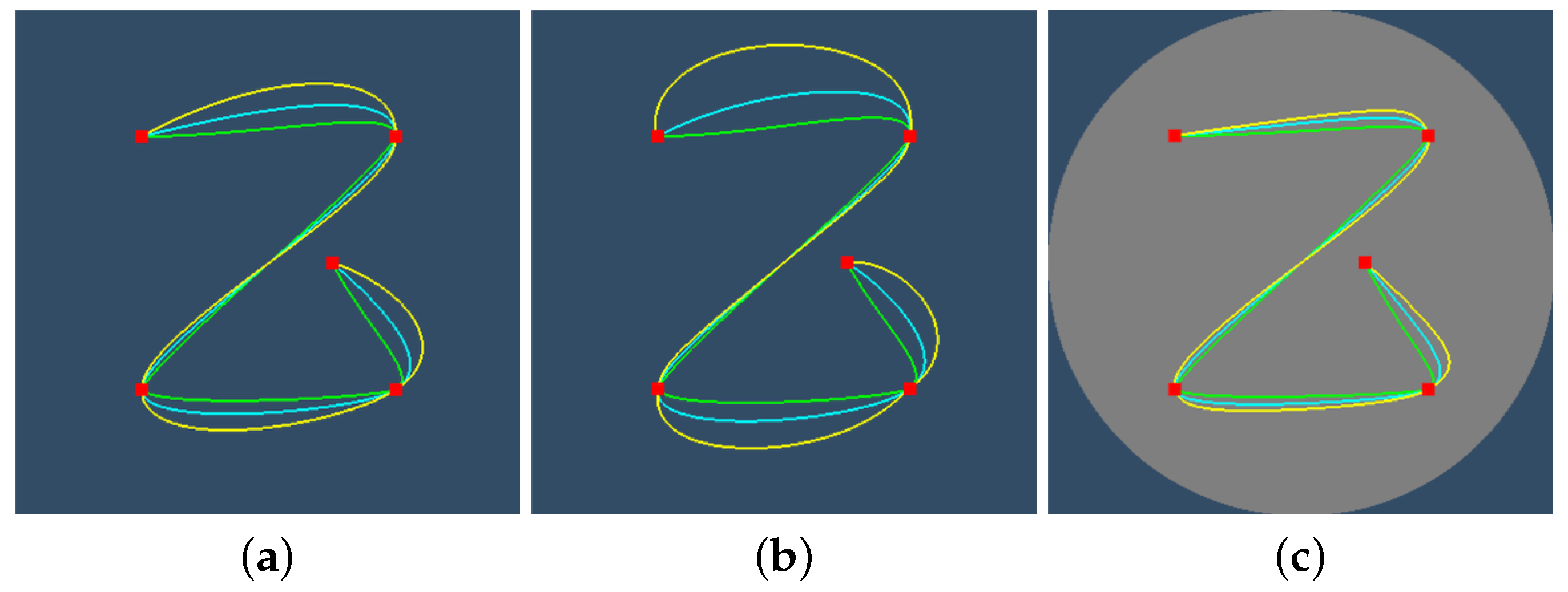
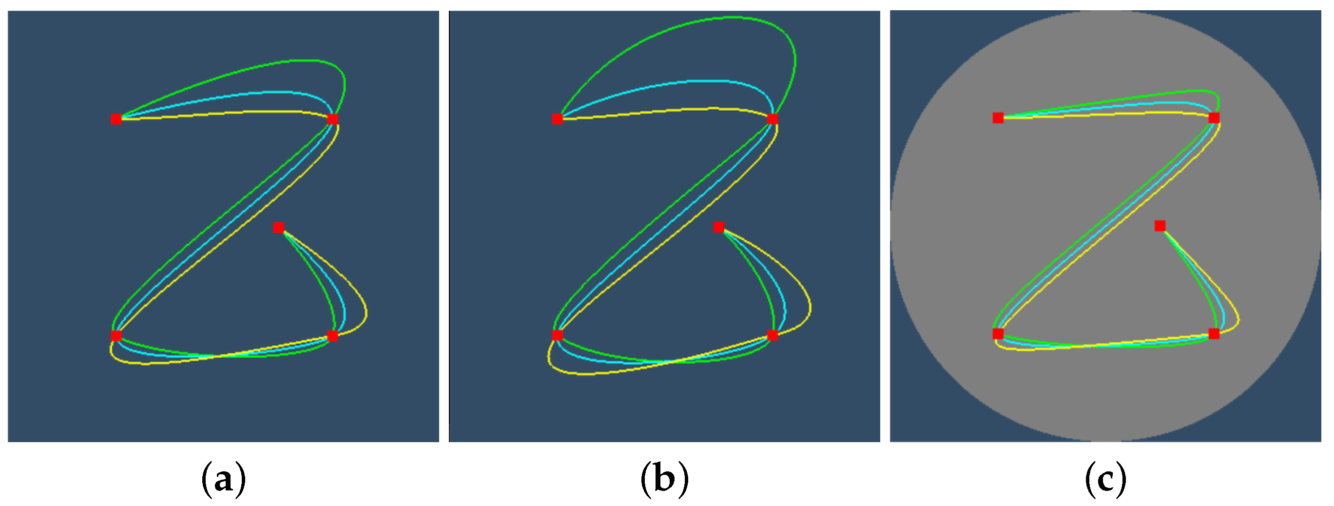
Figure 12 and Figure 13 examine the effects of the tension and bias parameters. If tension is increased, then the curvature in the control points is reduced, but it is increased farther from the control points. If bias is increased, the previous control point affects more the tangent in the current control point than the control point after the current one.

Figure 12.
The effect of tension parameter on the spline rendered with central projection (Klein’s model). Green, cyan, and yellow splines correspond to , , and , respectively. (a) Euclidean. (b) Elliptic. (c) Hyperbolic.
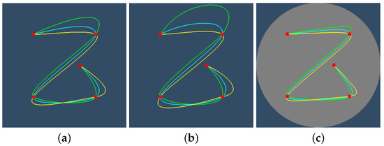
Figure 13.
The effect of bias parameter on the spline rendered with central projection (Klein’s model). Green, cyan, and yellow splines correspond to , , and , respectively. (a) Euclidean. (b) Elliptic. (c) Hyperbolic.
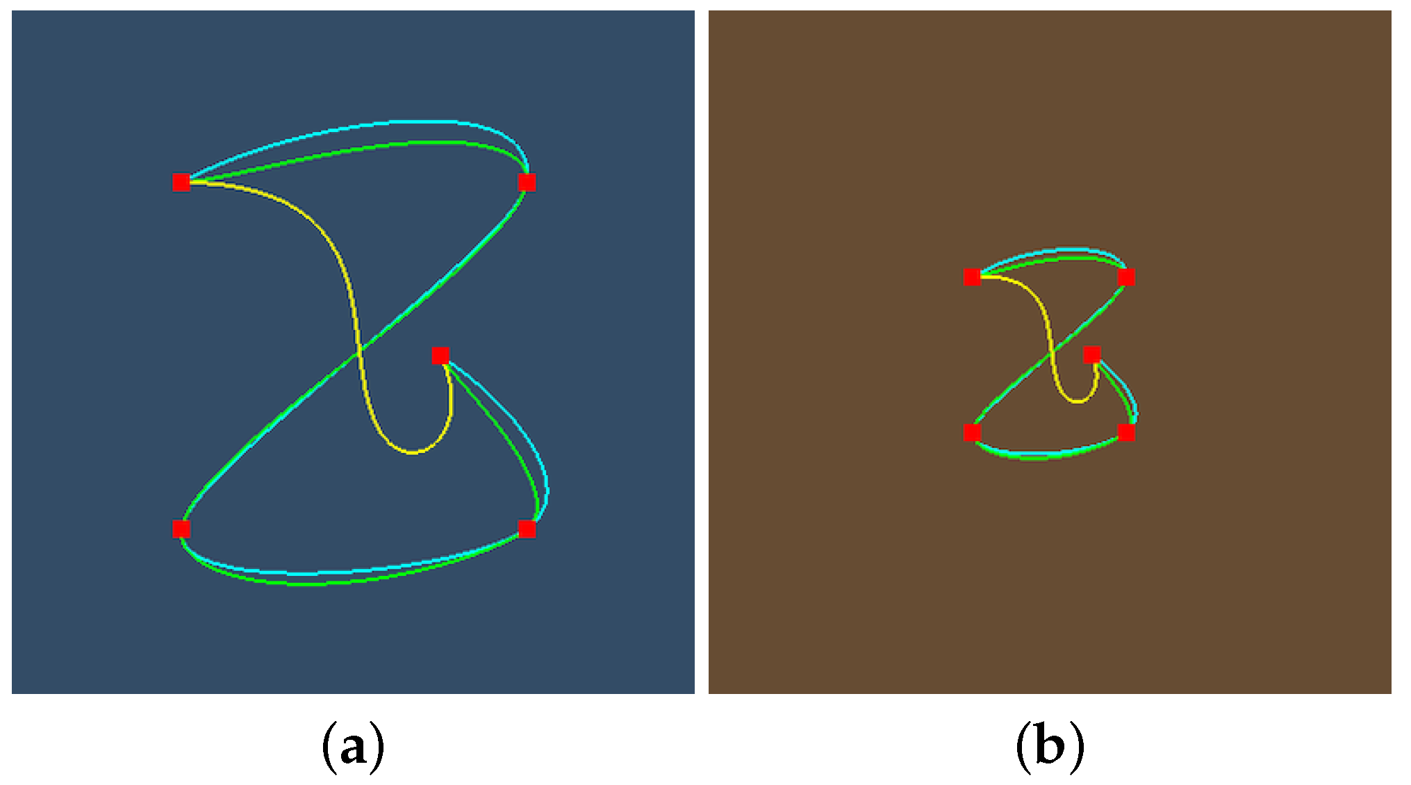
Figure 14 compares our proposed spherical spline to Spherical Quadrangle Interpolation (SQUAD) [19] and to the direct adaptation of de Casteljau’s algorithm [34] to the sphere. As the SQUAD works for quaternions, i.e., for the sphere in 4D, the z coordinate of the SQUAD solution is fixed to zero. To make the different solutions similar, we set the bias and tension parameters to one and assigned the natural numbers to the knot values since unlike our solution, de Casteljau’s method and the SQUAD both assume uniform parametrization. To find a spline point for a given parameter value, our method requires 1.1 μs computation time on a Intel i7 2.6GHz processor (Intel Corporation, Santa Clara, CA, USA), SQUAD 0.6 μs, and de Casteljau’s method 1.8 μs. This corresponds to the fact that our method needs seven geodesic interpolations per segment, SQUAD uses three, and de Casteljau’s approach evaluations, where N is the number of control points.
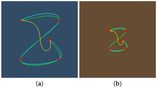
Figure 14.
Comparison of our proposed spline (cyan) to SQUAD (green) and to the application of the de Casteljau’s method (yellow) to define curves on the spherical surface. (a) Central projection. (b) Stereographic projection.
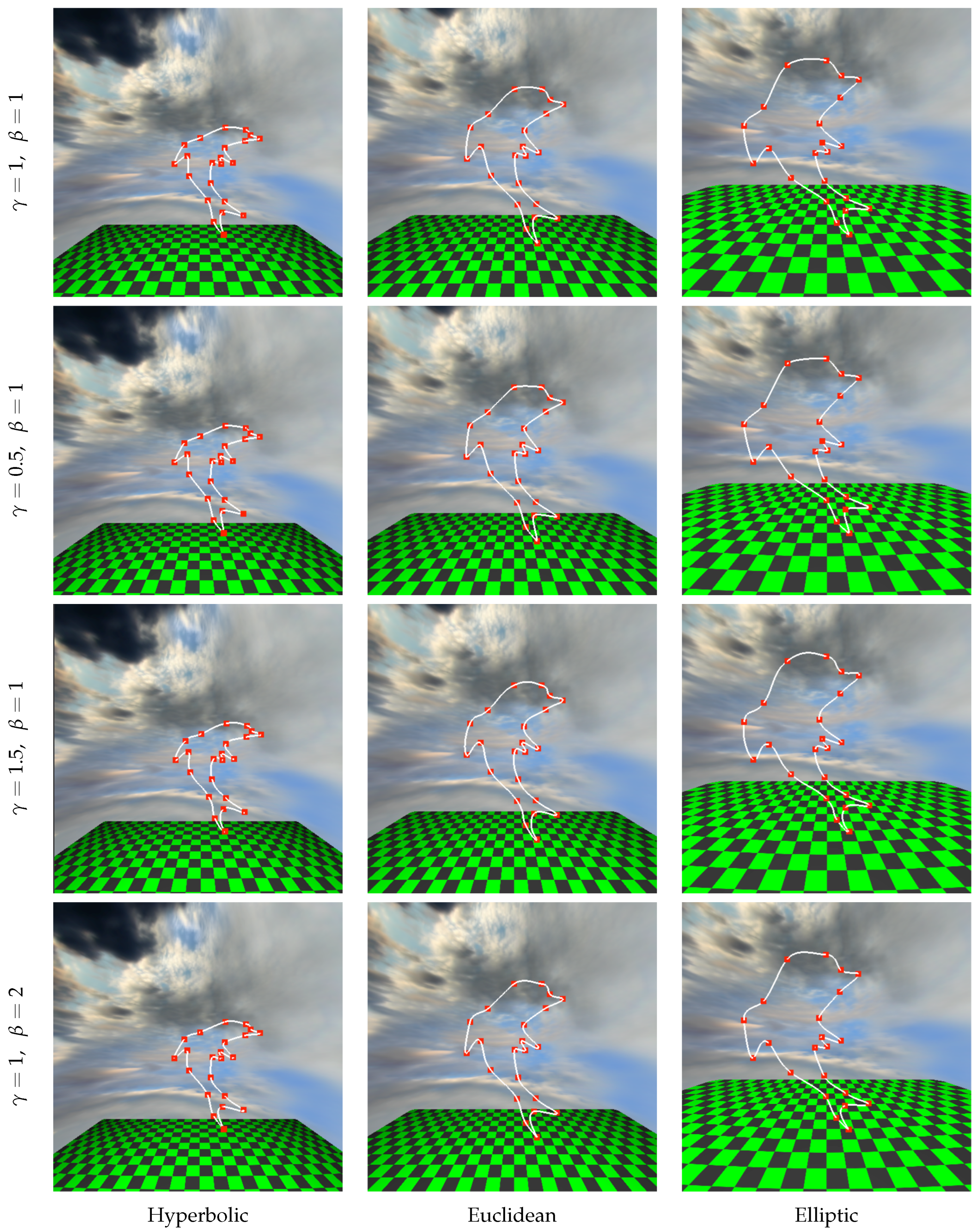
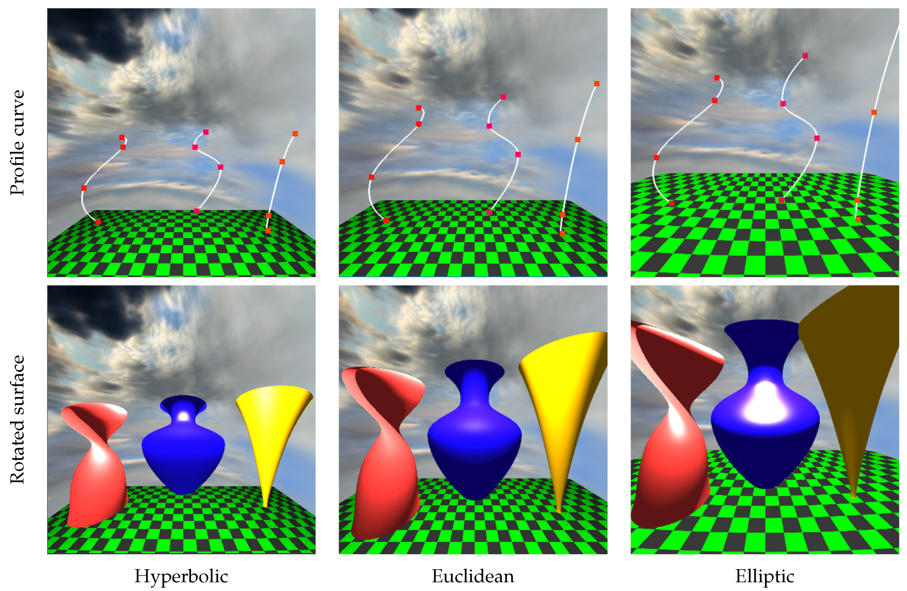
The 3D results are shown in a scene where objects are above a textured rectangle modeled as a ruled surface of two lines (Figure 15, Figure 16 and Figure 17). The stage rectangle and the objects above it are enclosed in a sky sphere, which is generated as a rotational surface. The eye is put to the geometry origin , the up direction of the camera is , while the view direction is , which are transformed to the canonical frame by the view transformation.
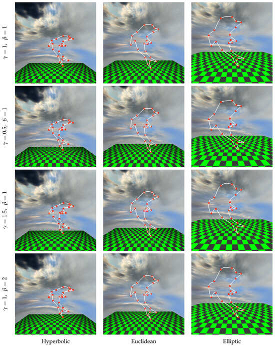
Figure 15.
Spline curve depicting the contour of a dolphin in the three model geometries of the columns. Rows correspond to different tension and bias settings.
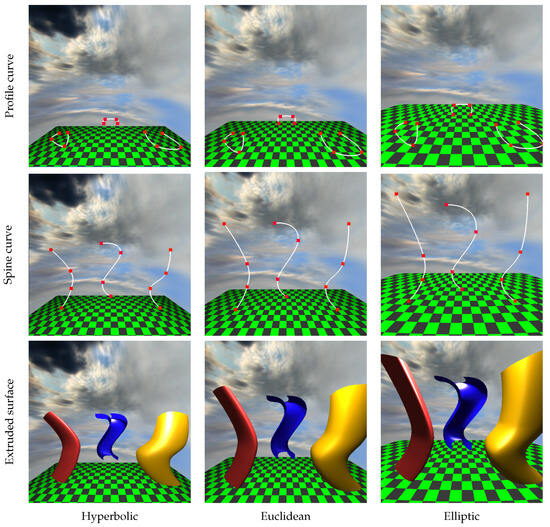
Figure 16.
Extruded surfaces.
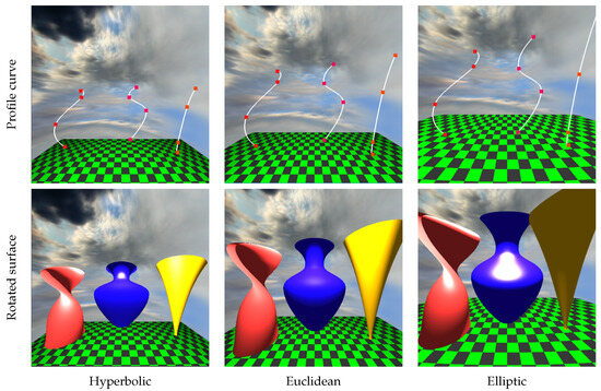
Figure 17.
Rotated surfaces. The profile curves are originally close to the geometry origin, where they are rotated and then translated their final position.
Note that the edges of the rectangular stage show up as Euclidean lines, although they are geodesics of curved spaces. The explanation is as follows: Before arriving at the coordinate system of the canonical camera, isometric transformations are applied that map geodesics to geodesics. A geodesic is the combination of two points (Equations (8) and (10)); thus, it is in the plane defined by the two combined points and the origin of the embedding space. Projection transformation is a homogeneous linear transformation that maps planes to planes. Finally, when the GPU executes the homogeneous division and obtains the points in 3D Cartesian coordinates, the intersection of the transformed plane and the plane of is determined, which is a Euclidean line.
To allow the comparison of scenes in different geometries, we tried to make them as similar as possible. The control points defining the spline surfaces are at the same distance and direction from the geometry origin in every examined geometric space.
Figure 1 also follows this setting, where classical surfaces like the cone, cylinder, and the sphere are modeled as rotational surfaces. Note that in hyperbolic geometry, visibility rays diverge faster than in Euclidean geometry; therefore, objects in the hyperbolic space look smaller. In elliptic geometry, however, visibility rays diverge first, and then, they converge; thus both close and far away, objects look large. Using the analogy of the Earth, if the eye position is at the North Pole, then objects close to the North and South Poles look large, while objects close to the equator look small.
Figure 15 is a spline curve approximating a dolphin contour in 3D. The rows correspond to different tension and bias settings and the columns to the three compared geometries. Unlike Figure 11, Figure 12, Figure 13 and Figure 14, the control points have been placed in the 3D curved spaces, or, in other words, in the 4D embedding space, making sure that the control point also belongs to the hyperbolic Euclidean and elliptic geometry. The proposed construction guarantees that all points of the the resulting splines belong to the respective space. The spline is drawn with different tension and bias parameters to demonstrate their effect in the 3D case. As in 2D, with smaller tension parameters , the curvature of the spline grows at the control points. With larger bias, we can emphasize the effect of the previous control point in the tangent of the curve at the current control point (control points are specified in clock-wise order in this figure).
Figure 16 presents extruded surfaces with their profile and the spine curves. Rows present the profile curve, the spine curve, and the final extruded surface obtained by sweeping the profile curve along the spine curve. Figure 17 displays the rotated surfaces together with their profile curves. The axis of rotation is in all examples.
The profile and the spine curves originally start close to the geometry origin, where the profile curve is extruded or rotated to generate the parametric surface. The parametric surface is finally translated to its position to separate the objects; then, the view transformation is applied to take the camera to its canonical settings.
When parametric surfaces are rendered, the normal vector of the surface is determined from the curve tangents according to Equation (26). When objects are transformed, the normal vectors are also updated. During illumination computation, we applied the diffuse-specular Phong–Blinn model depending on the transformed normal, illumination, and viewing directions. The unit viewing direction and the unit illumination direction at point are obtained from the equation of the geodesics:
where is the eye position, is the distance to the camera, is the position of the light source, and is the distance to the illuminated point.
4. Conclusions
We have presented a unified framework for constructing and rendering parametric curves and surfaces in constant-curvature geometries. Building on the embedding space model, we developed spline representations suitable for Euclidean, elliptic, and hyperbolic spaces, together with a recursive method for tangent calculation. Using these tools, we derived explicit formulas for extruded, rotational, and ruled surfaces, and addressed their tessellation and normal vector computation in the 4D embedding space.
On the rendering side, we demonstrated how cameras can be consistently defined via geodesic visibility lines and showed that view transformations reduce to matrix multiplications in the embedding space. This allowed us to describe both ray-based and object-based rendering methods and to integrate them with the incremental GPU pipeline through appropriate transformations. The resulting framework provides a foundation for efficiently modeling and visualizing curved geometries in real time.
Extending our techniques beyond constant-curvature spaces would require overcoming several challenges. Geodesic interpolation has no closed-form expression in general manifolds; so, extending spline curves to these spaces must involve numerical approximations. For special cases (e.g. matrix Lie groups, homogeneous spaces, etc.), the exponential and logarithmic maps—and thus geodesic interpolation—can still be computed via relatively inexpensive linear algebra. General manifolds have almost no global isometries; so, strict analogues of extruded and rotational surfaces can only exist in highly symmetric cases and, even then, only in distinguished directions. Nevertheless, manifold-based analogues of procedural surface definitions might be worthy of investigation, using, e.g., parallel transport or curve developments. Investigating alternatives to ray tracing for the visualization of Thurston geometries [46] is another promising avenue for related future research.
Author Contributions
Conceptualization, L.S.-K.; methodology, L.S.-K. and M.V.; software, A.F. and L.S.; validation, A.F.; formal analysis, L.S.-K. and M.V.; investigation, L.S.-K., A.F., L.S. and M.V.; writing—original draft preparation, L.S.-K.; writing—review and editing, A.F., L.S. and M.V.; visualization, A.F. and L.S. All authors have read and agreed to the published version of the manuscript.
Funding
This project has been supported by the National Research, Development and Innovation Office, Hungary (OTKA K-145970).
Informed Consent Statement
Not applicable.
Data Availability Statement
The original contributions presented in this study are included in the article. Further inquiries can be directed to the corresponding author.
Acknowledgments
GPUs used in this project are donations of NVIDIA.
Conflicts of Interest
The authors declare no conflicts of interest.
Abbreviations
The following abbreviations are used in this manuscript:
| GPU | Graphics Processing Unit |
| NDC | Normalized Device Coordinates |
| SLERP | Spherical Linear Interpolation |
| SQUAD | Spherical QUADrangle interpolation |
Appendix A. Proof of Equation (15)
Let us compute the time derivative of position selected by parameter on the line segment L:
The time derivative is denoted by Newton’s dot notation:
The first term (Equation (A1)) is simply the interpolation of the endpoint velocities, . In the second term (Equation (A2)), we have collected the factors of the derivative of distance between the endpoints, and in the third term (Equation (A3)), we collected the factors of .
Appendix A.1. Factor of (Equation (A2))
Applying the addition rule for sin or sinh,
we obtain
Appendix A.2. Factor of (Equation (A3))
The point at distance from on the line segment can be expressed both from the start and from the end points with their unit direction vectors:
which rearranges to
Thus, the factor of can be written as
Appendix A.3. Derivative of the Distance:
Now consider the derivative of the distance with respect to t. The distance d between points and satisfies
Differentiating both sides gives
Solving it for yields Equation (16).
Appendix B. Proof of Equation (21)
Let us substitute Equation (20) into the general formula of Equation (19). As the first three coordinates of and are equal and the fourth coordinate of is zero, we can use the following simplifying identity:
thus, the transformed point after two reflections is
Rearranging Equation (4) for that is in the geometry, we obtain
Scaler product is expressed using the definition of and :
Vector can be obtained as
With these, the double reflection formula can be further simplified:
References
- Szirmay-Kalos, L.; Magdics, M. Adapting Game Engines to Curved Spaces. Vis. Comput. 2021, 38, 4383–4395. [Google Scholar] [CrossRef]
- Mancinelli, C.; Puppo, E. Splines on manifolds: A survey. Comput. Aided Geom. Des. 2024, 112, 102349. [Google Scholar] [CrossRef]
- Karcher, H. Riemannian center of mass and mollifier smoothing. Commun. Pure Appl. Math. 1977, 30, 509–541. [Google Scholar] [CrossRef]
- Afsari, B. Means and Averaging on Riemannian Manifolds. Ph.D. Thesis, University of Maryland, College Park, MD, USA, 2009. [Google Scholar]
- Gabriel, S.A.; Kajiya, J.T. Spline interpolation in curved manifolds. In SIGGRAPH ’85, Course Notes for “State of the Art in Image Synthesis”; ACM: New York, NY, USA, 1985. [Google Scholar]
- Noakes, L.; Heinzinger, G.; Paden, B. Cubic splines on curved spaces. IMA J. Math. Control Inf. 1989, 6, 465–473. [Google Scholar] [CrossRef]
- Hofer, M.; Pottmann, H. Energy-minimizing splines in manifolds. In ACM SIGGRAPH 2004 Papers; ACM: New York, NY, USA, 2004; pp. 284–293. [Google Scholar] [CrossRef]
- Camarinha, M.; Silva Leite, F.; Crouch, P.E. High-order splines on Riemannian manifolds. Proc. Steklov Inst. Math. 2023, 321, 158–178. [Google Scholar] [CrossRef]
- Wallner, J. Geometric subdivision and multiscale transforms. In Handbook of Variational Methods for Nonlinear Geometric Data; Springer: Berlin/Heidelberg, Germany, 2020; pp. 121–152. [Google Scholar] [CrossRef]
- Mancinelli, C.; Nazzaro, G.; Pellacini, F.; Puppo, E. b/Surf: Interactive Bézier Splines on Surface Meshes. IEEE Trans. Vis. Comput. Graph. 2023, 29, 3419–3435. [Google Scholar] [CrossRef]
- Crane, K.; Livesu, M.; Puppo, E.; Qin, Y. A survey of algorithms for geodesic paths and distances. arXiv 2020, arXiv:2007.10430. [Google Scholar] [CrossRef]
- Boehm, W.; Müller, A. On de Casteljau’s algorithm. Comput. Aided Geom. Des. 1999, 16, 587–605. [Google Scholar] [CrossRef]
- De Boor, C. A Practical Guide to Splines; Springer: Berlin/Heidelberg, Germany, 1978; Volume 27. [Google Scholar]
- Barry, P.J.; Goldman, R.N. A recursive evaluation algorithm for a class of Catmull-Rom splines. ACM SIGGRAPH Comput. Graph. 1988, 22, 199–204. [Google Scholar] [CrossRef]
- Catmull, E.; Rom, R. A class of local interpolating splines. In Computer Aided Geometric Design; Elsevier: Amsterdam, The Netherlands, 1974; pp. 317–326. [Google Scholar] [CrossRef]
- Goldman, R. Pyramid Algorithms: A Dynamic Programming Approach to Curves and Surfaces for Geometric Modeling; Elsevier: Amsterdam, The Netherlands, 2002. [Google Scholar]
- Ramshaw, L. Blossoms are polar forms. Comput. Aided Geom. Des. 1989, 6, 323–358. [Google Scholar] [CrossRef]
- Shoemake, K. Animating rotation with quaternion curves. In Proceedings of the SIGGRAPH ’85: 12th Annual Conference on Computer Graphics and Interactive Technique; ACM Press: New York, NY, USA, 1985; pp. 245–254. [Google Scholar] [CrossRef]
- Dam, E.B.; Koch, M.; Lillholm, M. Quaternions, Interpolation and Animation; Technical Report DIKU-TR-98/5; Department of Computer Science, University of Copenhagen: Copenhagen, Denmark, 1998. [Google Scholar]
- Kim, M.J.; Kim, M.S.; Shin, S.Y. A general construction scheme for unit quaternion curves with simple high order derivatives. In Proceedings of the SIGGRAPH ’95: 22nd Annual Conference on Computer Graphics and Interactive Techniques, Los Angeles, CA, USA, 6–11 August 1995; ACM Press: New York, NY, USA, 1995; pp. 369–376. [Google Scholar] [CrossRef]
- Buss, S.R.; Fillmore, J.P. Spherical averages and applications to spherical splines and interpolation. ACM Trans. Graph. 2001, 20, 95–126. [Google Scholar] [CrossRef]
- Popiel, T.; Noakes, L. C2 spherical Bézier splines. Comput. Aided Geom. Des. 2006, 23, 261–275. [Google Scholar] [CrossRef]
- Hanson, A.J. Visualizing Quaternions; Morgan Kaufmann: Burlington, MA, USA, 2006. [Google Scholar]
- Geier, M. Splines in Euclidean Space and Beyond; Zenodo: Geneva, Switzerland, 2025. [Google Scholar] [CrossRef]
- Lin, A.; Walker, M. CAGD techniques for differentiable manifolds. In Algorithms for Approximation IV; Levesley, J., Anderson, I., Mason, J., Eds.; Huddlersfield University: Huddersfield, UK, 2001; pp. 36–43. [Google Scholar]
- Rockwood, A. Splossoms: Spherical Blossoms. In Advances in Computer Graphics; Springer: Berlin/Heidelberg, Germany, 2023; pp. 200–209. [Google Scholar] [CrossRef]
- Schaefer, S.; Goldman, R. Freeform curves on spheres of arbitrary dimension. In Proceedings of the Pacific Graphics, Macao, China, 12–14 October 2005; pp. 160–162. [Google Scholar]
- Kochanek, D.H.; Bartels, R.H. Interpolating splines with local tension, continuity, and bias control. ACM SIGGRAPH Comput. Graph. 1984, 18, 33–41. [Google Scholar] [CrossRef]
- Park, F.; Ravani, B. Bézier curves on Riemannian manifolds and Lie groups with kinematics applications. J. Mech. Des. 1995, 117, 36–40. [Google Scholar] [CrossRef]
- Crouch, P.; Kun, G.; Leite, F.S. The De Casteljau Algorithm on Lie Groups and Spheres. J. Dyn. Control Syst. 1999, 5, 397–429. [Google Scholar] [CrossRef]
- Popiel, T.; Noakes, L. Bézier curves and C2 interpolation in Riemannian manifolds. J. Approx. Theory 2007, 148, 111–127. [Google Scholar] [CrossRef]
- Nava-Yazdani, E.; Polthier, K. De Casteljau’s algorithm on manifolds. Comput. Aided Geom. Des. 2013, 30, 722–732. [Google Scholar] [CrossRef]
- Bogfjellmo, G.; Modin, K.; Verdier, O. A Numerical Algorithm for C2-Splines on Symmetric Spaces. SIAM J. Numer. Anal. 2018, 56, 2623–2647. [Google Scholar] [CrossRef]
- Hanik, M.; Nava-Yazdani, E.; von Tycowicz, C. De Casteljau’s algorithm in geometric data analysis: Theory and application. Comput. Aided Geom. Des. 2024, 110, 102288. [Google Scholar] [CrossRef]
- Ahanchaou, T.; Ikemakhen, A. Hyperbolic interpolatory geometric subdivision schemes. J. Comput. Appl. Math. 2022, 399, 113716. [Google Scholar] [CrossRef]
- Berger, P.; Laier, A.; Velho, L. An image-space algorithm for immersive views in 3-manifolds and orbifolds. Vis. Comput. 2015, 31, 93–104. [Google Scholar] [CrossRef]
- Velho, L.; Silva, V.d.; Novello, T. Immersive Visualization of the Classical Non-Euclidean Spaces using Real-Time Ray Tracing in VR. In Proceedings of the Graphics Interface, Toronto, ON, Canada, 28–29 May 2020; pp. 423–430. [Google Scholar] [CrossRef]
- Hart, J.C. Sphere Tracing: Simple Robust Antialiased Rendering of Distance-Based Implicit Surfaces. In SIGGRAPH 93 Course Notes: Modeling, Visualizing, and Animating Implicit Surfaces; ACM Press: New York, NY, USA, 1993; pp. 1–11. [Google Scholar]
- Weeks, J. Real-time rendering in curved spaces. IEEE Comput. Graph. Appl. 2002, 22, 90–99. [Google Scholar] [CrossRef]
- Gunn, C. Advances in Metric-neutral Visualization. In Proceedings of the 2nd International Workshop on Computer Graphics, Computer Vision and Mathematics, GraVisMa, Brno, Czech Republic, 7–10 September 2010; pp. 17–26. [Google Scholar]
- Martelli, B. An Introduction to Geometric Topology. arXiv 2016, arXiv:1610.02592. [Google Scholar]
- Loustau, B. Hyperbolic geometry. arXiv 2020, arXiv:2003.11180. [Google Scholar] [PubMed]
- Ghadami, R.; Rahebi, J.; Yayli, Y. Linear interpolation in Minkowski space. Int. J. Pure Appl. Math. 2012, 77, 469–484. [Google Scholar]
- Overhauser, A.W. Analytic Definition of Curves and Surfaces by Parabolic Blending; Technical Report SL 68–40; Mathematical and Theoretical Sciences Department, Scientific Laboratory, Ford Motor Company: Dearborn, MI, USA, 1968. [Google Scholar] [CrossRef]
- Blinn, J. Jim Blinn’s Corner: Notation, Notation, Notation; Morgan Kaufmann Publishers Inc.: Burlington, MA, USA, 2002. [Google Scholar]
- Novello, T.; da Silva, V.; Velho, L. Visualization of Nil, Sol, and SL2(R) geometries. Comput. Graph. 2020, 91, 219–231. [Google Scholar] [CrossRef]
Disclaimer/Publisher’s Note: The statements, opinions and data contained in all publications are solely those of the individual author(s) and contributor(s) and not of MDPI and/or the editor(s). MDPI and/or the editor(s) disclaim responsibility for any injury to people or property resulting from any ideas, methods, instructions or products referred to in the content. |
© 2025 by the authors. Licensee MDPI, Basel, Switzerland. This article is an open access article distributed under the terms and conditions of the Creative Commons Attribution (CC BY) license (https://creativecommons.org/licenses/by/4.0/).


