Scalable Time Series Causal Discovery with Approximate Causal Ordering

Abstract

Causal discovery in time series data presents a significant computational challenge. Standard algorithms are often prohibitively expensive for datasets with many variables or samples. This study introduces and validates a heuristic approximation of the VarLiNGAM algorithm to address this scalability problem. The standard VarLiNGAM method relies on an iterative refinement procedure for causal ordering that is computationally expensive. Our heuristic modifies this procedure by omitting the iterative refinement. This change permits a one-time precomputation of all necessary statistical values. The algorithmic modification reduces the time complexity of VarLiNGAM from $O\left(m^{3}n\right)$ to $O(m^{2}n+m^3)$ while keeping the space complexity at $O\left(m^2\right)$, where m is the number of variables and n is the number of samples. While an approximation, our approach retains VarLiNGAM’s essential structure and empirical reliability. On large-scale financial data with up to 400 variables, our algorithm achieves up to a 13.36× speedup over the standard implementation and an approximate 4.5× speedup over a GPU-accelerated version. Evaluations across medical time series analysis, IT service monitoring, and finance demonstrate the heuristic’s robustness and practical scalability. This work offers a validated balance between computational efficiency and discovery quality, making large-scale causal analysis feasible on personal computers.

1. Introduction

Time series causal discovery is the process of inferring cause-and-effect relationships from data points recorded in chronological order. The goal is to determine how variables influence one another, both at the same time (contemporaneous effects) and across different times (lagged effects).

While critical in many fields, time series causal discovery faces a fundamental scalability challenge: as datasets grow larger, computational demands quickly become prohibitive. This computational bottleneck severely limits the practical application of causal discovery to real-world problems. For example, the well-regarded VarLiNGAM algorithm, whose iterative nature results in $O\left(m^{3}n\right)$ complexity, becomes computationally intractable for datasets with many variables (m) or samples (n). On a typical laptop, analyzing just 100 variables can take hours, while 400 variables may require days of computation.

The core motivation for this work is to bridge this gap between algorithmic capability and practical scalability needs. We address this challenge by introducing a novel heuristic approximation of VarLiNGAM. This method intentionally modifies the standard iterative procedure by replacing the causal ordering refinement with an efficient one-time precomputation of necessary statistical values. This algorithmic change is based on the central hypothesis that for many complex time series, the initial dependency structure contains sufficient information to identify the correct causal ordering without iterative updates. This change reduces the complexity to $O(m^{2}n+m^3)$. While this approach is an approximation and thus sacrifices a degree of theoretical exactness, it retains the essential structure of the original algorithm and, as our experiments show, its empirical reliability.

Our method relies on an efficient precomputation strategy, which is a well-known technique for performance enhancement in data analysis. For example, preprocessing for approximate Bayesian computation in image analysis can reduce the average runtime required for model fitting from 71 h to 7 min [1].

The key contributions of this work are as follows:

• A computational bottleneck analysis of the VarLiNGAM algorithm, identifying the iterative data refinement within its DirectLiNGAM estimator as the primary source of its $O\left(m^{3}n\right)$ complexity.
• The design and analysis of a novel heuristic, which approximates the standard procedure by replacing iterative refinement with an approximation and precomputation strategy. This reduces the theoretical time complexity to $O(m^{2}n+m^3)$.
• An evaluation of the proposed heuristic on diverse synthetic and real-world datasets. The results demonstrate significant speedups (up to 13× over the official CPU implementation [2] and 4.5× over a GPU version [3]) with a negligible cost to discovery accuracy.

Our method offers a validated balance between computational efficiency and causal discovery quality, extending the feasibility of applying causal discovery to large-scale, real-world problems using standard hardware resources. The source code of the proposed approach is available online (Code repository: https://github.com/ceguo/varlingam-heuristic, accessed on 1 September 2025).

2. Background and Related Work

Causal discovery from time series data is concerned with inferring directed causal graphs from multivariate observational data. This task is distinct from analysis in independent and identically distributed (i.i.d.) settings because it must explicitly account for temporal dependencies, where a variable at one point in time can influence another variable at a future point in time [4]. The typical output of these methods is a directed graph that provides a map of a system’s causal mechanisms.

Time series causal discovery demonstrates substantial practical impact across diverse domains. In financial computing, these methods enable asset pricing analysis [5], enhance factor investing strategies [6], and optimize portfolio construction [7]. Healthcare applications include brain connectivity analysis for neurological disorders [8,9], medical time series generation [10], and adverse event identification in clinical settings [11]. Earth system sciences leverage causal discovery for interactive climate visualization [12], regime-oriented climate modeling [13], and wind speed forecasting in renewable energy systems [14].

2.1. Time Series Causal Discovery Methods

Time series causal discovery methods can be categorized into several types: (i) Granger causality [15] and its variants [16,17,18]; (ii) information-theoretic methods [19,20,21,22]; (iii) constraint-based methods [23,24,25,26]; and (iv) function-based methods [27,28,29,30,31,32,33]. More recently, deep learning-based methods emerge as a powerful alternative. Examples include Neural Granger Causality [34], which uses neural networks for non-linear Granger tests; Temporal Causal Discovery Framework (TCDF) [35], which uses attention-based CNNs to find relationships and lags; and CausalFormer [36], an interpretable transformer for temporal causal graphs.

This study focuses on function-based methods. These methods assume a specific data-generating process. By imposing structural constraints on the relationships between variables, these models can often identify a unique causal graph where other methods might only identify a class of equivalent graphs. A prominent family of function-based methods is the Linear Non-Gaussian Acyclic Model (LiNGAM). LiNGAM-based methods assume that the causal relationships between variables are linear, the system is acyclic, and the external noise sources affecting each variable are independent and non-Gaussian [27,28]. The non-Gaussianity assumption is critical, as it breaks the statistical symmetry that makes linear Gaussian models non-identifiable. Under these assumptions, the causal structure can be identified using techniques like Independent Component Analysis (ICA) [37]. The Vector Autoregressive LiNGAM (VarLiNGAM) model extends this framework to time series data [38]. It works by first fitting a standard Vector Autoregressive (VAR) model to account for the time-lagged causal influences. It then applies the LiNGAM algorithm to the residuals of the VAR model to discover the contemporaneous, or instantaneous, causal structure.

Our VARLiNGAM acceleration approach has a distinct position in the time series causal discovery field. While constraint-based methods like tsFCI are good at handling high-dimensional data and confounders but require extensive conditional independence testing, and continuous optimization approaches like DYNOTEARS offer scalability but assume specific noise models, VARLiNGAM provides a middle ground. It uses the non-Gaussian assumption for identifiability while maintaining computational efficiency through our proposed heuristic acceleration. This positions our work as particularly suitable for scenarios where non-Gaussian assumptions hold and moderate-scale problems require both accuracy and efficiency.

2.2. Scalability and Acceleration

Hardware-centric acceleration aims to reduce the execution time of existing algorithms by using specialized processors. GPU acceleration is a common strategy. For constraint-based methods, GPUs are used to parallelize the large number of required conditional independence tests [39,40]. For function-based methods, GPUs are used to accelerate the intensive matrix operations involved in algorithms like LiNGAM [3,41]. For even larger-scale problems, some work explores the use of supercomputers to distribute the workload across thousands of nodes [42]. Other research focuses on using Field-Programmable Gate Arrays (FPGAs) to create custom hardware pipelines for specific bottlenecks, such as the generation of candidate condition sets for CI tests [43,44,45]. These hardware-centric solutions are effective but depend on the availability of specialized and often costly computing resources.

In contrast, our work explores a purely algorithmic path to scalability. Instead of using more computational resources to execute the same number of operations faster, we modify the algorithm itself to fundamentally reduce the total operation count. This makes our contribution distinct from, and complementary to, existing work on hardware acceleration. Our focus is on improving performance on standard, widely accessible hardware, which is a different but equally important direction for making large-scale causal discovery more practical for a broader community of researchers and practitioners.

3. Bottleneck Analysis of DirectLiNGAM

As part of the VarLiNGAM procedure, DirectLiNGAM is the de facto method to find the causal ordering and contemporaneous causal graph [46]. It operates iteratively, identifying and removing the most exogenous variable from a set of candidates in each pass. This iterative refinement is both the source of its accuracy and its high computational cost.

The DirectLiNGAM algorithm is designed to find the causal ordering of variables through an iterative search procedure. The time complexity of VarLiNGAM is equivalent to that of DirectLiNGAM, due to the high efficiency of VAR. Each main loop of DirectLiNGAM identifies the most exogenous variable among a set of current candidates. The following is a detailed breakdown of the steps performed within a single loop to find the k-th variable in the causal ordering, $c_k$, along with an analysis of the computational cost of each step. In this analysis, $m_k$ denotes the number of remaining variables at the start of the iteration, and n is the number of samples.

• Standardization: First, the current data matrix $X^{(k-1)}$, which contains the $m_k$ variables yet to be ordered, is standardized so that each column has a mean of zero and a variance of one. This ensures that the scale of the variables does not affect the subsequent calculations.
  Execution Time: This step requires calculating the mean and standard deviation for each of the $m_k$ columns. Both operations have a complexity of $O\left(n\right)$ for a single column. Therefore, the total time complexity for standardizing the entire matrix is $O(m_k·n)$.
• Pairwise Residual Calculation: For every pair of variables ($x_i,x_j$) with indices in the current set $U^{(k-1)}$, the linear regression residual is computed. The residual $r_{i\leftarrow j}$ represents the part of $x_i$ that cannot be linearly explained by $x_j$. It is calculated as

  $$r_{i\leftarrow j}=x_i-{\displaystyle \frac{\mathrm{cov}(x_i,x_j)}{\mathrm{var}\left(x_j\right)}}{x}_j$$

  (1)
  Execution Time: This is a computationally intensive step. For each of the $O\left(m_k^2\right)$ pairs of variables, calculating the covariance and variance takes $O\left(n\right)$ time, and the subsequent vector operations also take $O\left(n\right)$ time. Consequently, the total time complexity for this step is $O(m_k^2·n)$.
• Scoring via Mutual Information: A measure of dependence, $T_{i\leftarrow j}$, is calculated for each pair of variables. This score approximates the mutual information between a variable and its residual after regressing on another. Using an entropy approximation $H(·)$, it is defined as

  $$T_{i\leftarrow j}=H\left(x_i\right)-H\left(r_{i\leftarrow j}\right)$$

  (2)
  A lower value of $T_{i\leftarrow j}$ indicates that $x_j$ explains less of the information in $x_i$, suggesting $x_i$ is more independent of $x_j$.
  Execution Time: The entropy calculation for a single vector of length n has a complexity of $O\left(n\right)$. This step requires calculating the entropy for all $m_k$ variables and all $O\left(m_k^2\right)$ residuals computed in the previous step. The total time complexity is therefore dominated by the calculation of residual entropies, resulting in a cost of $O(m_k^2·n)$.
• Variable Selection: For each candidate variable $x_i$, an aggregate score $M_i$ is computed by summing a function of the pairwise scores against all other remaining variables $x_j$:

  $$M_i=\sum _{j\in U^{(k-1)},j\ne i}f(T_{i\leftarrow j},T_{j\leftarrow i})$$

  (3)
  The variable $c_k$ with the score indicating maximum overall independence is selected as the k-th variable in the causal ordering.
  Execution Time: For each of the $m_k$ variables, computing the aggregate score involves summing $m_k-1$ terms. Assuming the function f is $O\left(1\right)$, this takes $O\left(m_k\right)$ time per variable. The total time to calculate all aggregate scores is $O\left(m_k^2\right)$. This is computationally less significant compared to the previous steps.
• Iterative Data Refinement: This is the crucial step that ensures the correctness of subsequent iterations. The algorithm prepares the data matrix for the next loop, $X^{\left(k\right)}$, by removing the influence of the just-found variable $c_k$ from all other remaining variables. For each remaining variable index j, the corresponding column in the new data matrix is updated with its residual:

  $$x_j^{\left(k\right)}=r_{j\leftarrow c_k}^{(k-1)}=x_j^{(k-1)}-{\displaystyle \frac{\mathrm{cov}(x_j^{(k-1)},x_{c_k}^{(k-1)})}{\mathrm{var}\left(x_{c_k}^{(k-1)}\right)}}{x}_{c_k}^{(k-1)}$$

  (4)
  The set of candidate indices is also updated, $U^{\left(k\right)}=U^{(k-1)}\setminus \left\{c_k\right\}$, and the process repeats to find the next variable, $c_{k+1}$.
  Execution Time: This step involves $m_k-1$ residual calculations. Since each residual calculation takes $O\left(n\right)$ time, the total time complexity for this refinement step is $O(m_k·n)$.

The fifth step, iterative data refinement, is the fundamental bottleneck, because the entire data matrix X is updated in every one of the m main iterations. In each iteration, all pairwise residuals and entropy calculations must be re-computed from scratch. This nested computational structure is what leads to the high overall complexity of $O\left(m^{3}n\right)$.

4. Proposed Approach: Approximate Causal Ordering

Our work focuses on accelerating the core bottleneck of the VarLiNGAM algorithm: the estimation of the instantaneous causal matrix $B_0$ using its default estimator, DirectLiNGAM [46]. To address this, we propose a novel heuristic approximation that modifies the causal ordering algorithm in DirectLiNGAM for VarLiNGAM.

4.1. Rationale of Approximation

A main purpose of DirectLiNGAM algorithm’s iterative refinement is to isolate direct causal effects from statistical associations. When variables exhibit causal relationships, their statistical dependencies reflect both direct and indirect influences. For example, if A causes B, and B causes C, then A and C will be statistically dependent even without a direct A → C link. The iterative causal order search process addresses this by sequentially removing the influence of identified causal variables. After identifying A as most exogenous, the algorithm removes A’s influence from all remaining variables before proceeding. This ensures that subsequent causal assessments are based on residual relationships rather than confounded total effects.

Customized for time series data, VarLiNGAM employs a VAR model as its initial step to remove temporal dependencies. The VAR model subtracts predictable past influences from each variable, generating residuals that capture instantaneous events at each time point. These residuals serve as a proxy for instantaneous causal relationships, effectively cleaning the data of temporal confounds.

Our heuristic is based on the hypothesis that this VAR preprocessing provides sufficient cleaning that the remaining instantaneous structure can be identified without iterative refinement. Specifically, we claim that for many time series systems, the post-VAR residuals contain an adequate signal that precomputed pairwise relationships can substitute for iteratively refined assessments. Note that our approach is specifically tailored to time series data where VAR preprocessing provides the necessary foundation. Whether this approximation is effective in non-time series scenarios remains unclear.

4.2. Algorithmic Modification and Precomputation

The implementation of our heuristic fundamentally alters the program flow. Instead of an iterative refinement process, it adopts a precompute-and-lookup strategy.

• Precomputation of Marginal Entropies: Before the search for causal ordering begins, the entropy of each standardized column $x_i$ from the original data matrix X is calculated once and stored in an array of size m.
• Precomputation of Residual Entropies: All $m\times (m-1)$ pairwise residuals, $r_{i\leftarrow j}$ for all $i\ne j$, are calculated from the single, original, unaltered data matrix X. The entropy of each of these residuals is then computed and stored in an $m\times m$ matrix.
• Accelerated Causal Ordering Search: The main loop to find the causal ordering proceeds for m iterations. However, in each iteration, it performs its search over the same, static set of precomputed entropy values. The scoring calculation (Step 3 and 4 of the original method) is reduced from a series of vector operations to a few memory lookups from the precomputed arrays. Crucially, the data matrix X is never updated.

Algorithm 1 outlines our heuristic, where the expensive calculations are moved outside the main loop into a precomputation phase. The main loop no longer contains any residual or entropy calculations, and most importantly, it lacks the data update step.

Algorithm 1 Proposed Heuristic Causal Order Search

1:  Input: Data matrix X, initial set of indices $U=\{1,\dots ,m\}$ 2:  Output: Causal order K 3:  $E_x\leftarrow \mathrm{precomputeMarginalEntropies}\left(X\right)$ 4:  $E_r\leftarrow \mathrm{precomputeResidualEntropies}\left(X\right)$ 5:  $K\leftarrow \left[\right]$ 6:  for $k=1$ to m do 7:      Find $c_k\in U$ that minimizes the dependence score M in Equation (3) by looking up values in $E_x$ and $E_r$. 8:      Append $c_k$ to K. 9:      $U\leftarrow U\setminus \left\{c_k\right\}$ 10: end for 11: return K

This algorithmic change directly impacts the complexity. The two precomputation steps have a combined complexity of $O(mn+m^{2}n)=O\left(m^{2}n\right)$. The main search loop, which runs m times, now only performs $O\left(m^2\right)$ work per iteration (for pairwise score lookups and comparisons), resulting in a total search complexity of $O\left(m^3\right)$. The final complexity of our heuristic is the sum of these parts, $O(m^{2}n+m^3)$, which is substantially lower than the original’s $O\left(m^{3}n\right)$, since the number of variables m is typically of the order ${10}^3$ and beyond [47]. Also, since the approximation only needs to store the dependence score M for each pair of variables, the space complexity is $O\left(m^2\right)$, which is the same as the original VarLiNGAM algorithm.

4.3. Implementation Details

The proposed method employs a fast approximation to differential entropy based on maximum entropy approximations and following the original DirectLiNGAM implementation. Also, following DirectLiNGAM, our algorithm computes an aggregated score for each candidate variable i according to

$$M_i=\sum _{j\ne i}min{(0,\mathrm{DMI}(i,j))}^2$$

(5)

where the difference in mutual information is defined as

$$\mathrm{DMI}(i,j)=(H\left(X_j\right)+H\left(X_i\right|X_j))-(H\left(X_i\right)+H\left(X_j\right|X_i))$$

(6)

The variable with the maximum aggregated score $M_i$ is selected as the next variable in the causal order. This scoring rule forms the core of the DirectLiNGAM approach, with ties handled through the subsequent Adaptive Lasso regularization step.

The preprocessing pipeline consists of timestamp removal, standardization, entropy precomputation, and residual entropy precomputation. Data columns identified as timestamps are excluded from analysis. All variables are then standardized using $X=(X-\mu )/\sigma$ where $\mu$ and $\sigma$ are the sample mean and standard deviation. Differential entropies for all variables are computed once before the main algorithm, and all pairwise residual entropies are precomputed to avoid repeated calculations during search. No additional detrending, differencing, or rolling standardization is applied to the time series data.

Key hyperparameters are set as follows throughout the experiments. VAR order selection uses the Bayesian Information Criterion (BIC). The lag structure is set to 1 for fMRI datasets and 3 for IT monitoring datasets to balance model complexity with numerical stability. Adaptive Lasso uses $\gamma =1.0$, and pruning is disabled.

The following mechanisms are used to handle multicollinearity and numerical stability. Data standardization ensures comparable scales across all variables before processing. Adaptive Lasso regularization employs a two-stage weighted approach with BIC model selection to handle variable selection and multicollinearity simultaneously. Variables with zero coefficients after Lasso regularization are excluded from the model.

5. Evaluation

5.1. Experimental Setup

To assess the performance of our heuristic, we use three standard metrics: F1-score [46], Structural Hamming Distance (SHD) [48], and Structural Intervention Distance (SID) [48]. We conduct experiments on a variety of datasets to test performance under different conditions. To ensure a fair comparison of computational performance, both the original and our proposed implementations are developed in Python 3.12 using identical numerical libraries such as NumPy and SciPy. No explicit multi-threading or other parallel frameworks are used in the CPU implementations, meaning that the observed speedup is attributable solely to the change in the algorithm’s design. Since real-world causal discovery tasks are often executed on personal computers [49], we use a laptop for the evaluation. The laptop has an Intel (Santa Clara, CA, USA) Core Ultra 7 155H CPU and 32GB DDR5 memory without a dedicated GPU. For reference implementations that must run on GPUs, we use a different machine that contains an NVIDIA (Santa Clara, CA, USA) Tesla T4 GPU.

5.2. Evaluation with Synthetic Data

We perform two sets of experiments on synthetic data to analyze the performance of our heuristic against the original algorithm under controlled conditions. Note that we mainly use the synthetic data to evaluate scalability while the accuracy results are for reference only. This is because synthetic data generation can inadvertently favor the assumptions of the method being tested [50].

The results, shown in Figure 1 and Figure 2, illustrate the practical trade-offs between computation time and discovery accuracy.

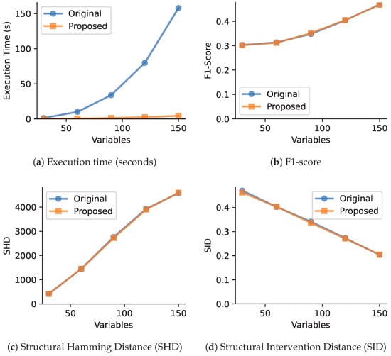
Figure 1. Performance comparison between original and proposed VARLiNGAM methods with varying number of variables (30, 60, 90, 120, 150) and fixed sample size (1000). The proposed method demonstrates high computational efficiency while maintaining comparable causal discovery accuracy.

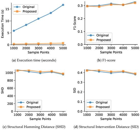
Figure 2. Performance comparison between original and proposed VARLiNGAM methods with varying sample sizes (1000, 2000, 3000, 4000, 5000) and fixed number of variables (50). The proposed method maintains consistent computational advantages across all sample sizes while achieving similar causal discovery performance.

• Fixed sample size ($n=1000$) with increasing number of variables. As shown in Figure 1, the execution time of the original search step grows rapidly, which is consistent with its high computational complexity. In contrast, our heuristic’s search time remains nearly constant. While the precomputation step introduces some overhead, the overall time-saving is substantial. Note that a practical dataset may have a smaller sample size, so the acceleration can be less significant. The next two charts show that this efficiency gain is achieved with almost no loss in accuracy, as the difference in F1-scores between the original algorithm and our heuristic is less than 0.01.
• Fixed number of variables ($m=50$) with increasing sample size. Figure 2 shows that the original algorithm’s search time grows linearly with the number of samples, while our heuristic’s search time is again constant. The total runtime for our method is significantly lower across all sample sizes. The last two figures in the second row confirm that the accuracy is again comparable. It is worth noting that for very small datasets, the time saved by the faster search loop might not fully compensate for the initial overhead of the precomputation step. Our method demonstrates its primary advantages in the situations where the original algorithm becomes computationally intensive.

5.3. Real-World Data with Ground Truth

We evaluate the heuristic on an fMRI benchmark from neuroscience [4] and the IT monitoring benchmark from [51]. The fMRI benchmark contains 28 datasets. For brevity, we use five datasets with the largest numbers of variables. The IT monitoring dataset represents the largest real-world dataset with ground truth available for VarLiNGAM evaluation. While CausalRivers [52] is a larger dataset, it proves fundamentally incompatible with VarLiNGAM-based approaches since both the standard algorithm and our heuristic achieve negligible accuracy on this data. Including such comparisons provides no meaningful insights regarding our approximation’s relative performance.

As shown in Table 1, our method achieves a significant speedup on both benchmarks, reducing the total execution time by more than half. This efficiency gain comes with negligible change in the F1-score, SHD and SID, which remain well within the standard deviation of the original method’s performance. Also, on both benchmarks, the proposed heuristic consistently reduces execution times.

Table 1. Performance comparison between the original VARLiNGAM method (Orig.) and the proposed heuristic method (Prop.) across 12 datasets. Results show F1-score (unitless, higher is better), Structural Hamming Distance (SHD, count of edge differences, lower is better), Structural Intervention Distance (SID, unitless measure of causal structure difference, lower is better), and execution time with speedup (SU). The $\Delta$ columns show the difference (Proposed–Original) with blue indicating improvements and orange indicating degradations. fMRI datasets use lag = 1, IT monitoring datasets use lag = 3.

	F1-Score			SHD			SID			Time
Dataset	Orig.	Prop.	Δ	Orig.	Prop.	Δ	Orig.	Prop.	Δ	Raw (s)	SU
fMRI-2	0.3590	0.3621	+0.0031	75	74	−1	9.4	9.4	0	0.042	3.8×
fMRI-3	0.2683	0.2739	+0.0056	180	175	−5	15.9	15.9	0	0.111	5.3×
fMRI-4	0.0889	0.0863	−0.0026	2193	2203	+10	65.5	65.5	0	3.662	16.4×
fMRI-11	0.3455	0.3486	+0.0032	72	71	−1	9.4	9.4	0	0.037	3.4×
fMRI-17	0.3478	0.3448	−0.0030	75	76	+1	9.4	9.4	0	0.037	3.4×
MoM1	0.1026	0.1026	0	35	35	0	6.1	6.1	0	0.017	2.3×
MoM2	0.1500	0.1500	0	34	34	0	5.4	5.4	0	0.017	2.3×
Web1	0.2258	0.2295	+0.0037	48	47	−1	6.1	5.6	−0.5	0.193	3.7×
Web2	0.2750	0.2785	+0.0035	58	57	−1	8.4	8.4	0	0.220	4.3×
Antivirus1	0.1955	0.1926	−0.0029	107	109	+2	10.1	10.1	0	0.125	4.6×
Antivirus2	0.2090	0.2105	+0.0016	106	105	−1	10.2	10.2	0	0.126	4.6×
Ingestion	0.1905	0.1613	−0.0292	51	52	+1	7.3	7.3	0	0.043	3.0×

The robustness of the proposed heuristic under assumption deviations is demonstrated through our evaluation on real-world datasets, which naturally exhibit violations of the strict non-Gaussian and linear assumptions underlying VARLiNGAM. The fMRI datasets contain noise that introduces near-Gaussian components, while the IT monitoring datasets exhibit system nonlinearities, feedback loops, and confounding factors inherent to complex distributed systems. Despite these realistic assumption violations, the proposed method maintains good accuracy across all twelve datasets, while achieving consistent speedups.

5.4. Real-World Datasets Without Ground Truth

To test scalability on a challenging, high-dimensional problem, we use S&P500 stock data [38]. We benchmark our CPU version against the standard CPU implementation from the lingam package [2] and a GPU-accelerated version of the original algorithm [3]. The results are shown in Table 2. The speed advantage of our method grows dramatically with the number of variables. For 400 variables, our heuristic is 13.36 times faster than the original CPU algorithm and 4.55 times faster than the GPU implementation. The original algorithm takes nearly 6 h to run, while our heuristic finishes in under 27 min on the same hardware. This shows that for achieving scalability, a proper algorithmic design can be more effective than hardware acceleration of an inefficient algorithm. The accessibility of running such large-scale analyses on a standard laptop is a key practical outcome of our work.

Table 2. Execution time (seconds) and speedup on the S&P500 dataset. ‘Original₁’ refers to the CPU version from [2], ‘GPU₂’ to the GPU version from [3], and `Heuristic CPU₃’ is our version.

	Execution Time (s)			Speedup
Design	Orig. CPU1	GPU2	Prop. CPU3	SU13	SU23
$N_{\mathrm{variables}}=25$	4.03	8.83	1.88	2.14×	4.69×
$N_{\mathrm{variables}}=50$	27.31	32.89	8.70	3.14×	3.78×
$N_{\mathrm{variables}}=100$	230.06	168.04	44.54	5.17×	3.77×
$N_{\mathrm{variables}}=200$	1660.57	1030.17	226.80	7.32×	4.54×
$N_{\mathrm{variables}}=400$	21,404.76	7291.09	1601.80	13.36×	4.55×

To isolate the sources of computational gains in the proposed heuristic, we conduct a focused ablation study on a large-scale dataset. Using the 400-variable setting, we evaluate three configurations to show the performance cost of removing each optimization component:

• The proposed method with both precomputation components active runs in 1601.80 s.
• Disabling only the marginal entropy precomputation increases the execution time to 1927.25 s.
• Disabling only the residual entropy precomputation significantly increases the execution time to 5959.71 s.

The analysis demonstrates that precomputing residual entropies is the primary source of the speedup. Removing this single optimization increases the execution time from approximately 27 min to nearly 1.5 h. This confirms that the dominant computational bottleneck in the original method is the repeated calculation of conditional entropies, $H\left(X_i\right|X_j)$, during the causal ordering search, which our heuristic’s main optimization eliminates.

6. Discussion

Our work successfully demonstrates the value of a heuristic approach to a computationally difficult problem. This section contextualizes our contribution, discusses the inherent limitations of our method, and analyzes the practical trade-offs related to scalability and system resources.

6.1. Primary Contribution in Context

The main contribution of this work is the design and validation of a new point in the design space for causal discovery algorithms. While precomputation is a known optimization technique, its application to VarLiNGAM requires a deliberate algorithmic modification: the omission of the iterative data refinement step in DirectLiNGAM. The novelty of our contribution is not the act of precomputation itself, but the empirical demonstration that this specific and aggressive approximation is highly effective within the VarLiNGAM context.

Our findings position this algorithmic approximation as a practical alternative to purely hardware-centric acceleration. Our efficient algorithm on standard hardware can outperform the original algorithm running on a specialized processor like a GPU. For example, in the experiments described in Section 5.3 with the S&P500 stock data, the proposed approach running on the CPU achieves up to 4.55 times speedup over the original VarLiNGAM running on the GPU. This suggests that for practitioners without access to high-performance computing resources, exploring algorithmic heuristics can be a more accessible and effective path to achieving scalability. The impact of this work is most significant for users with standard, commodity hardware, as it enables them to perform large-scale causal discovery that was previously infeasible.

6.2. Limitations of the Heuristic Approach

The primary limitation is the heuristic nature of the algorithm. By omitting the iterative residualization step, we lose the theoretical guarantee of correctness that the original DirectLiNGAM algorithm provides. Our experiments suggest that the accuracy loss is minimal in many practical cases. However, there exist specific data-generating processes where our heuristic may fail to find the correct causal ordering while the original algorithm succeeds.

For example, consider a chain structure A → B → C with strong contemporaneous causal effects. In this scenario, variable B receives direct influence from A and also influences C. The original VarLiNGAM algorithm first identifies A as the most exogenous variable and removes its influence from the data before proceeding. This iterative refinement ensures that when evaluating the B–C relationship in subsequent steps, the algorithm sees only the direct effect of B on C. However, our heuristic computes all relationships from the original, unrefined data. When assessing the independence between B and C, it observes the total statistical dependency, which includes both the direct effect B → C and the indirect effect A → B → C. This conflation of direct and indirect effects can lead to misidentification of the causal ordering. Also, a longer chain structure may have more negative impact.

Moreover, this paper focuses on the algorithmic trade-off between speed and accuracy. It does not attempt to explain the domain-specific mechanisms behind the causal relationships discovered in the real-world datasets. The tool we develop is intended to be used by domain experts who can provide the necessary context and interpretation for the resulting causal graphs.

6.3. Scalability and Resource Trade-Offs

Our method achieves its speedup by altering the pattern of computation and memory access. While the asymptotic space complexity remains $O\left(m^2\right)$, our heuristic trades repeated calculations for persistent memory storage. By precomputing and storing all pairwise residual entropies in an $O\left(m^2\right)$ table upfront, it eliminates the need for computationally expensive calculations in each iteration of the search loop. For the datasets used in our experiments, this memory footprint is minor on modern computers. However, for systems with severely limited memory resources, or for problems with an extremely large number of variables (many thousands), this could become a bottleneck. In such scenarios, memory optimization techniques could be considered, such as using lower-precision floating-point numbers or developing a hybrid strategy that only precomputes a subset of the most frequently accessed values.

Regarding performance in high-dimensional settings, our heuristic offers a significant improvement. However, its scalability is not infinite. While we reduce the dependency on the number of samples n, the complexity still includes an $O\left(m^3\right)$ term from the search phase. As the number of variables m grows, this term eventually becomes the new computational bottleneck, particularly for datasets where $m>>n$. Even so, improving the complexity from $O\left(m^{3}n\right)$ to $O(m^{2}n+m^3)$ means a substantial step forward in making higher-dimensional time series causal discovery more tractable.

7. Conclusions and Future Work

This study introduces and validates a novel heuristic approximation of the VarLiNGAM algorithm, designed to overcome the computational barriers that limit the use of causal discovery on large-scale time series data. By making an algorithmic change to the core DirectLiNGAM estimator, specifically by omitting the iterative data refinement step, we enable an efficient precomputation strategy. This modification reduces the computational complexity significantly, resulting in major speedups that make analysis of datasets with hundreds of variables feasible on a standard laptop. Our evaluation demonstrates that this gain in efficiency comes at a negligible cost to empirical accuracy across a variety of synthetic and real-world problems. This work highlights that for certain classes of complex algorithms, a well-designed algorithmic approximation can be a more effective and accessible path to scalability than pure hardware acceleration.

Future work includes a systematic performance evaluation across different structural patterns, including chains, stars, and dense networks, to characterize when this approximation breaks down. Future work also addresses the evaluation trade-off in causal discovery acceleration: small datasets with ground truth enable accuracy assessment but cannot demonstrate meaningful speedups due to GPU overhead, while large datasets that showcase acceleration lack ground truth for accuracy evaluation. Establishing proxy quality metrics for large real-world datasets can enable comprehensive runtime vs. accuracy analyses and provide clearer guidance on when to employ different acceleration strategies.

References

- Moores, M.T.; Drovandi, C.C.; Mengersen, K.; Robert, C.P. Pre-processing for approximate Bayesian computation in image analysis. Stat. Comput. 2015, 25, 23–33. [Google Scholar] [CrossRef]
- Ikeuchi, T.; Ide, M.; Zeng, Y.; Maeda, T.N.; Shimizu, S. Python Package for Causal Discovery Based on LiNGAM. J. Mach. Learn. Res. 2023, 24, 1–8. [Google Scholar]
- Akinwande, V.; Kolter, J.Z. AcceleratedLiNGAM: Learning Causal DAGs at the Speed of GPUs. arXiv 2024, arXiv:2403.03772. [Google Scholar]
- Assaad, C.K.; Devijver, E.; Gaussier, E. Survey and Evaluation of Causal Discovery Methods for Time Series. J. Artif. Int. Res. 2022, 73, 767–819. [Google Scholar] [CrossRef]
- Haddad, V.; He, Z.; Huebner, P.; Kondor, P.; Loualiche, E. Causal Inference for Asset Pricing. 2025. Available online: https://papers.ssrn.com/sol3/papers.cfm?abstract_id=5187305 (accessed on 1 September 2025).
- de Prado, M.M.L. Causal Factor Investing: Can Factor Investing Become Scientific? Cambridge University Press: Cambridge, UK, 2023. [Google Scholar]
- Rodriguez Dominguez, A. Causal Portfolio Optimization: Principles and Sensitivity-Based Solutions. arXiv 2025, arXiv:2504.05743. [Google Scholar] [CrossRef]
- Ji, J.; Zhang, Z.; Han, L.; Liu, J. MetaCAE: Causal autoencoder with meta-knowledge transfer for brain effective connectivity estimation. Comput. Biol. Med. 2024, 170, 107940. [Google Scholar] [CrossRef]
- Seth, A.K.; Barrett, A.B.; Barnett, L. Granger Causality Analysis in Neuroscience and Neuroimaging. J. Neurosci. 2015, 35, 3293–3297. [Google Scholar] [CrossRef]
- Li, H.; Yu, S.; Principe, J. Causal recurrent variational autoencoder for medical time series generation. In Proceedings of the AAAI Conference on Artificial Intelligence, Washington, DC, USA, 7–14 February 2023; Volume 37, pp. 8562–8570. [Google Scholar]
- Wei, S.; Xie, Y.; Josef, C.S.; Kamaleswaran, R. Granger causal chain discovery for sepsis-associated derangements via continuous-time Hawkes processes. In Proceedings of the 29th ACM SIGKDD Conference on Knowledge Discovery and Data Mining, Long Beach, CA, USA, 6–10 August 2023; pp. 2536–2546. [Google Scholar]
- Melkas, L.; Savvides, R.; Chandramouli, S.H.; Mäkelä, J.; Nieminen, T.; Mammarella, I.; Puolamäki, K. Interactive causal structure discovery in earth system sciences. In Proceedings of the KDD’21 Workshop on Causal Discovery, PMLR, Singapore, 15 August 2021; pp. 3–25. [Google Scholar]
- Karmouche, S.; Galytska, E.; Runge, J.; Meehl, G.A.; Phillips, A.S.; Weigel, K.; Eyring, V. Regime-oriented causal model evaluation of Atlantic–Pacific teleconnections in CMIP6. Earth Syst. Dyn. 2023, 14, 309–344. [Google Scholar] [CrossRef]
- Hlavackova-Schindler, K.; Hoxhallari, K.; Caumel Morales, L.; Schicker, I.; Plant, C. Causal discovery among wind-related variables in a wind farm under extreme wind speed scenarios: Comparison of results using Granger causality and interactive k-means clustering. In Proceedings of the EGU General Assembly Conference Abstracts, Vienna, Austria, 14–19 April 2024; p. 6584. [Google Scholar]
- Granger, C.W.J. Investigating Causal Relations by Econometric Models and Cross-spectral Methods. In Essays in Econometrics: Collected Papers of Clive W. J. Granger; Ghysels, E., Swanson, N.R., Watson, M.W., Eds.; Cambridge University Press: Cambridge, UK, 2001; pp. 31–47. [Google Scholar]
- Arize, A.C. Determinants of Income Velocity in the United Kingdom: Multivariate Granger Causality. Am. Econ. 1993, 37, 40–45. [Google Scholar] [CrossRef]
- Chen, Y.; Rangarajan, G.; Feng, J.; Ding, M. Analyzing Multiple Nonlinear Time Series with Extended Granger Causality. Phys. Lett. A 2004, 324, 26–35. [Google Scholar] [CrossRef]
- Geweke, J. Measurement of Linear Dependence and Feedback Between Multiple Time Series. J. Am. Stat. Assoc. 1982, 77, 304–313. [Google Scholar] [CrossRef]
- Schreiber, T. Measuring Information Transfer. Phys. Rev. Lett. 2000, 85, 461–464. [Google Scholar] [CrossRef]
- Bossomaier, T.; Barnett, L.; Harré, M.; Lizier, J.T. Transfer Entropy. In An Introduction to Transfer Entropy: Information Flow in Complex Systems; Springer International Publishing: Cham, Switzerland, 2016; pp. 65–95. [Google Scholar] [CrossRef]
- Kraskov, A.; Stögbauer, H.; Grassberger, P. Estimating Mutual Information. Phys. Rev. E 2004, 69, 066138. [Google Scholar] [CrossRef] [PubMed]
- Barnett, L.; Barrett, A.; Seth, A. Granger Causality and Transfer Entropy Are Equivalent for Gaussian Variables. Phys. Rev. Lett. 2009, 103, 238701. [Google Scholar] [CrossRef] [PubMed]
- Spirtes, P.; Glymour, C.; Scheines, R. Causation, Prediction, and Search; The MIT Press: Cambridge, MA, USA, 2001. [Google Scholar] [CrossRef]
- Kalisch, M.; Bühlmann, P. Estimating High-dimensional Directed Acyclic Graphs with the PC-algorithm. J. Mach. Learn. Res. 2007, 8, 613–636. [Google Scholar]
- Runge, J.; Nowack, P.; Kretschmer, M.; Flaxman, S.; Sejdinovic, D. Detecting and Quantifying Causal Associations in Large Nonlinear Time Series Datasets. Sci. Adv. 2019, 5, eaau4996. [Google Scholar] [CrossRef] [PubMed]
- Entner, D.; Hoyer, P.O. On Causal Discovery from Time Series Data Using FCI. In Proceedings of the 5th European Workshop on Probabilistic Graphical Models, Helsinki, Finland, 13–15 September 2010; Myllymäki, P., Roos, T., Jaakkola, T., Eds.; pp. 121–128. [Google Scholar]
- Shimizu, S.; Hoyer, P.O.; Hyvärinen, A.; Kerminen, A. A Linear Non-Gaussian Acyclic Model for Causal Discovery. J. Mach. Learn. Res. 2006, 7, 2003–2030. [Google Scholar]
- Shimizu, S. Lingam: Non-Gaussian Methods for Estimating Causal Structures. Behaviormetrika 2014, 41, 65–98. [Google Scholar] [CrossRef]
- Hoyer, P.; Janzing, D.; Mooij, J.M.; Peters, J.; Schölkopf, B. Nonlinear Causal Discovery with Additive Noise Models. In Advances in Neural Information Processing Systems 2008; Koller, D., Schuurmans, D., Bengio, Y., Bottou, L., Eds.; Curran Associates, Inc.: Red Hook, NY, USA, 2008; Volume 21. [Google Scholar]
- Mooij, J.; Janzing, D.; Peters, J.; Schölkopf, B. Regression by Dependence Minimization and its Application to Causal Inference in Additive Noise Models. In Proceedings of the 26th Annual International Conference on Machine Learning (ICML ’09), New York, NY, USA, 14–18 June 2009; pp. 745–752. [Google Scholar] [CrossRef]
- Nowzohour, C.; Bühlmann, P. Score-based Causal Learning in Additive Noise Models. Statistics 2015, 50, 471–485. [Google Scholar] [CrossRef]
- Zhang, K.; Hyvarinen, A. On the Identifiability of the Post-Nonlinear Causal Model. arXiv 2012, arXiv:1205.2599. [Google Scholar] [CrossRef]
- Pamfil, R.; Sriwattanaworachai, N.; Desai, S.; Pilgerstorfer, P.; Georgatzis, K.; Beaumont, P.; Aragam, B. DYNOTEARS: Structure Learning from Time-Series Data. In Proceedings of the Twenty Third International Conference on Artificial Intelligence and Statistics, Online, 26–28 August 2020; Chiappa, S., Calandra, R., Eds.; Proceedings of Machine Learning Research. Volume 108, pp. 1595–1605. [Google Scholar]
- Tank, A.; Covert, I.; Foti, N.; Shojaie, A.; Fox, E.B. Neural Granger Causality. IEEE Trans. Pattern Anal. Mach. Intell. 2022, 44, 4267–4279. [Google Scholar] [CrossRef]
- Nauta, M.; Bucur, D.; Seifert, C. Causal Discovery with Attention-based Convolutional Neural Networks. Mach. Learn. Knowl. Extr. 2019, 1, 312–340. [Google Scholar] [CrossRef]
- Kong, L.; Li, W.; Yang, H.; Zhang, Y.; Guan, J.; Zhou, S. CausalFormer: An Interpretable Transformer for Temporal Causal Discovery. IEEE Trans. Knowl. Data Eng. 2025, 37, 102–115. [Google Scholar] [CrossRef]
- Hyvärinen, A.; Karhunen, J.; Oja, E. Independent Component Analysis; Adaptive and Cognitive Dynamic Systems: Signal Processing, Learning, Communications and Control; Wiley: Hoboken, NJ, USA, 2004. [Google Scholar]
- Hyvärinen, A.; Zhang, K.; Shimizu, S.; Hoyer, P. Estimation of a Structural Vector Autoregression Model Using Non-Gaussianity. J. Mach. Learn. Res. 2010, 11, 1709–1731. [Google Scholar]
- Zarebavani, B.; Jafarinejad, F.; Hashemi, M.; Salehkaleybar, S. cuPC: CUDA-Based Parallel PC Algorithm for Causal Structure Learning on GPU. IEEE Trans. Parallel Distrib. Syst. 2020, 31, 530–542. [Google Scholar] [CrossRef]
- Hagedorn, C.; Huegle, J. GPU-Accelerated Constraint-based Causal Structure Learning for Discrete Data. In Proceedings of the 2021 SIAM International Conference on Data Mining (SDM), SIAM, Virtual Event, 29 April–1 May 2021; pp. 37–45. [Google Scholar]
- Shahbazinia, A.; Salehkaleybar, S.; Hashemi, M. Paralingam: Parallel Causal Structure Learning for Linear Non-gaussian Acyclic Models. J. Parallel Distrib. Comput. 2023, 176, 114–127. [Google Scholar] [CrossRef]
- Matsuda, K.; Kurihara, K.; Kawakami, K.; Yamazaki, M.; Yamada, F.; Tabaru, T.; Yokoyama, K. Accelerating LiNGAM Causal Discovery with Massive Parallel Execution on Supercomputer Fugaku. IEICE Trans. Inf. Syst. 2022, E105.D, 2032–2039. [Google Scholar] [CrossRef]
- Guo, C.; Luk, W. Accelerating Constraint-based Causal Discovery by Shifting Speed Bottleneck. In Proceedings of the 2022 ACM/SIGDA International Symposium on Field-Programmable Gate Arrays (FPGA ’22), New York, NY, USA, 27 February–1 March 2022; pp. 169–179. [Google Scholar] [CrossRef]
- Guo, C.; Cupello, D.; Luk, W.; Levine, J.; Warren, A.; Brookes, P. FPGA-Accelerated Causal Discovery with Conditional Independence Test Prioritization. In Proceedings of the 2023 33rd International Conference on Field-Programmable Logic and Applications (FPL), Gothenburg, Sweden, 4–8 September 2023; pp. 182–188. [Google Scholar]
- Guo, C.; Luk, W.; Warren, A.; Levine, J.; Brookes, P. Co-Design of Algorithm and FPGA Accelerator for Conditional Independence Test. In Proceedings of the 2023 IEEE 34th International Conference on Application-specific Systems, Architectures and Processors (ASAP), Porto, Portugal, 19–21 July 2023; pp. 102–109. [Google Scholar]
- Shimizu, S.; Inazumi, T.; Sogawa, Y.; Hyvärinen, A.; Kawahara, Y.; Washio, T.; Hoyer, P.O.; Bollen, K. DirectLiNGAM: A Direct Method for Learning a Linear Non-Gaussian Structural Equation Model. J. Mach. Learn. Res. 2011, 12, 1225–1248. [Google Scholar]
- Jeon, S.Y.; Ryou, H.S.; Kim, Y.; Oh, K.J. Using change-point detection to identify structural changes in stock market: Application to Russell 2000. Quant. Bio-Sci. 2020, 39, 61–69. [Google Scholar]
- Peters, J.; Bühlmann, P. Structural Intervention Distance for Evaluating Causal Graphs. Neural Comput. 2015, 27, 771–799. [Google Scholar] [CrossRef]
- Le, T.D.; Hoang, T.; Li, J.; Liu, L.; Liu, H.; Hu, S. A fast PC algorithm for high dimensional causal discovery with multi-core PCs. IEEE/ACM Trans. Comput. Biol. Bioinform. 2016, 16, 1483–1495. [Google Scholar] [CrossRef] [PubMed]
- Reisach, A.; Seiler, C.; Weichwald, S. Beware of the simulated dag! causal discovery benchmarks may be easy to game. Adv. Neural Inf. Process. Syst. 2021, 34, 27772–27784. [Google Scholar]
- Aït-Bachir, A.; Assaad, C.K.; de Bignicourt, C.; Devijver, E.; Ferreira, S.; Gaussier, E.; Mohanna, H.; Zan, L. Case Studies of Causal Discovery from IT Monitoring Time Series. arXiv 2023, arXiv:2307.15678. [Google Scholar] [CrossRef]
- Gideon, S.; Maha, S.; Jan, B.; Niklas, P.; Joachim, D. CausalRivers-Scaling up benchmarking of causal discovery for real-world time-series. In Proceedings of the Thirteenth International Conference on Learning Representations, Singapore, 24–28 April 2025. [Google Scholar]
Disclaimer/Publisher’s Note: The statements, opinions and data contained in all publications are solely those of the individual author(s) and contributor(s) and not of MDPI and/or the editor(s). MDPI and/or the editor(s) disclaim responsibility for any injury to people or property resulting from any ideas, methods, instructions or products referred to in the content. |
© 2025 by the authors. Licensee MDPI, Basel, Switzerland. This article is an open access article distributed under the terms and conditions of the Creative Commons Attribution (CC BY) license (https://creativecommons.org/licenses/by/4.0/).