Fictitious Point Technique Based on Finite-Difference Method for 2.5D Direct-Current Resistivity Forward Problem

Abstract

With the widespread application of the direct-current resistivity method, searching for accurate and fast-forward algorithms has become the focus of research for geophysicists and engineers. Three-dimensional forward modeling can be the best way to identify geo-electrical anomalies but are hampered by computational limitations because of the large amount of data. A practical compromise, or even alternative, is represented by 2.5D modeling characterized using a 3D source in a 2D medium. Thus, we develop a 2.5D direct-current resistivity forward modeling algorithm. The algorithm incorporates the finite-difference approximation and fictitious point technique that can improve the efficiency and accuracy of numerical simulation. Firstly, from the boundary value problem of the electric potential generated by the point source, the discrete expressions of the governing equation are derived from the finite-difference approach. The numerical solutions of the discrete electric potential are calculated after the approximate treatment of the boundary conditions with a finite-difference method based on a fictitious point scheme. Secondly, through the simulation of a homogeneous half-space model and a one-dimensional model, and compared with the analytical results, the correctness and stability of the finite-difference forward algorithm are verified. Lastly, through the numerical simulation for a two-dimensional model, 2.5D direct-current sounding responses are summarized, which can provide a qualitative interpretation of field data.

1. Introduction

Direct-current resistivity is a surface geophysical method that can provide essential information for investigating subsurface geological structures by injecting electric current into the Earth and measuring the corresponding voltage. It can find applications in mineral resource exploration [1,2,3], environmental and urban geological surveys [4,5,6,7], and humanitarian geophysics [8]. Regular two-dimensional (2.5D) and three-dimensional (3D) surveys are now conducted. In these multidimensional cases, the interpretation of apparent resistivity data requires an accurate modeling approach. The computer resources required for 3D direct-current resistivity simulation severely restrict the practical applicability of any automated interpretation technology. The 3D direct-current resistivity forward modeling can be expected not only from the direct development of 3D algorithms but also from a reasonable compromise between the degree of required forward model complexity and the level of computer resources consumed. A practical compromise, or even alternative, is represented by 2.5D direct-current resistivity modeling characterized by the use of a 3D point source in a 2D geological structure.

Numerical modeling approaches have been developed and applied for direct-current resistivity forward modeling, such as finite-difference and finite-element methods, as the approximation of partial differential equations (Poisson equation or Helmholtz equation) [9]. The finite-difference method is an effective approach for solving partial differential equations by approximating second-order derivatives with a different scheme in the governing equation [10,11,12,13]. Several studies have explored the efficiency and accuracy of finite-difference methods for direct-current resistivity modeling [14,15,16,17,18]. However, it is not easy to calculate the exact space-domain electrical potential. The finite-element method is another numerical approach for the direct-current resistivity modeling, which solves the variational problem in integral form for the electrical potential, and then carries out a numerical integration [19,20,21,22]. The finite-element methods use complex real-world information, such as topography and bathymetry, when building density models, and improve the flexibility of 2D, 2.5D, or 3D discretization domains [23]. Unfortunately, high-accuracy direct-current resistivity modeling needs fine grids, which will lead to high computational costs [24]. Additionally, there are some other numerical schemes for the 2.5D direct-current resistivity modeling, such as the finite-volume method [25], the element-free Galerkin method [26], and the boundary-element method [27]. These methods provide a good research basis for both numerical simulations of 2D geo-electrical models and numerical simulations in related geophysical disciplines.

In this work, the finite-difference method to incorporate a fictitious point technique was developed for 2.5D direct-current resistivity modeling, which is different to the traditional finite-difference numerical method without a fictitious point scheme. The time consumption for solving the finite-difference linear equation system without the fictitious point technique would be longer than that of the finite-difference method with the fictitious point approach. In addition, the finite-difference forward algorithm incorporated with the fictitious point technique will give more accurate approximate results than the traditional finite-difference approach, especially in dealing with the 3D direct-current resistivity forward problem.

The rest of this paper is arranged as follows. The boundary value problem for the 2.5D wavenumber domain potential is introduced in Section 2. Section 3 is devoted to presenting the high-performance implementation of the finite-difference algorithm with a fictitious point technique for 2.5D direct-current resistivity modeling. In Section 4, several numerical experiments are used to confirm the accuracy and efficiency of the forward algorithm. The main discussions and conclusions are summarized in Section 5 and Section 6, respectively. Appendix A contains the MATLAB code for 2.5D direct-current resistivity modeling. Appendix B and Appendix C present the mathematical expressions of analytical solutions in homogenous half-space and two-layer resistivity models, respectively.

2. Statement of 2.5D Direct-Current Resistivity Forward Problem

The 3D space-domain electrical potential $u\left(x,y,z\right)$ generated by a point source located at (x_s, 0, 0) on the ground surface can be described as a Poisson equation [28]:

$$\nabla \cdot \left[\sigma \left(x,y,z\right)\nabla u\left(x,y,z\right)\right]=-Q\left(x,y,z\right)\delta \left(x_s\right)\delta \left(y_s\right)\delta \left(z_s\right),\mathrm{in}\Omega$$

(1)

where $\delta$ is the unit Dirac (impulse) function, $Q\left(x,y,z\right)$ denotes the constant steady-state current density specified at a point, $\Omega$ presents the computational domain, and $\left(x_s,y_s,z_s\right)$ indicate the coordinates of the point source of charge injected in the x-y-z space.

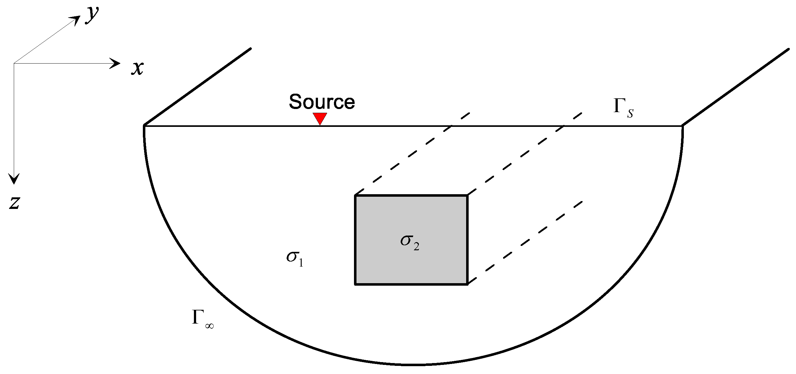
At the air–earth interface ${\Gamma }_S$, shown in Figure 1, the electrical potential satisfies the following Neumann boundary condition:

$${\left.\frac{\partial u}{\partial n}\right|}_{{\Gamma }_S}=0.$$

(2)

Figure 1. Model of 2D geo-electrical structure.

On the distant boundary or truncated boundary ${\Gamma }_{\infty }$, the Neumann boundary can be also applied. It can be written as

$${\left.\frac{\partial u}{\partial n}\right|}_{{\Gamma }_{\infty }}=0,$$

(3)

where n is the outward-pointing normal vector on the truncated boundary ${\Gamma }_{\infty }$.

Assuming the strike of the geological structure is aligned with the y-axis, the above problem can be simplified and efficiently simulated in the Fourier domain. The forward Fourier-cosine transform is defined as follows:

$$U\left(x,\lambda ,z\right)={\displaystyle {\int }_0^{+\infty }u\left(x,y,z\right)\cos \left(\lambda y\right)\mathrm{d}y},$$

(4)

where $\lambda$ presents the wavenumber and $U\left(x,\lambda ,z\right)$ denotes the wavenumber domain electrical potential. Applying the forward Fourier-cosine transform to Equations (1)–(3), after some calculation, the Helmholtz boundary value problem for the wavenumber domain electrical potential $U\left(x,\lambda ,z\right)$ can be expressed as

$$\left.\begin{array}{l}\left[\frac{\partial }{\partial x}\left(\sigma \frac{\partial U}{\partial x}\right)+\frac{\partial }{\partial z}\left(\sigma \frac{\partial U}{\partial z}\right)\right]-{\lambda }^2\sigma U=-Q\cdot \delta \left(x_s\right)\delta \left(z_s\right)\\ {\left.\frac{\partial U}{\partial n}\right|}_{{\Gamma }_S}=0\\ {\left.\frac{\partial U}{\partial n}\right|}_{{\Gamma }_{\infty }}=0\end{array}\right\},$$

(5)

where ${\Gamma }_S$ and ${\Gamma }_{\infty }$ denote the corresponding 2D boundary of the computational domain.

The constant steady-state current density Q in $\left(x,\lambda ,z\right)$ space can be related to the current density I injected at $\left(x_s,z_s\right)$ by

$$Q=\frac{I}{2\Delta A},$$

where $\Delta A$ denotes a representative area in the x-z plane related to the injection source point $\left(x_s,z_s\right)$.

3. Methodology

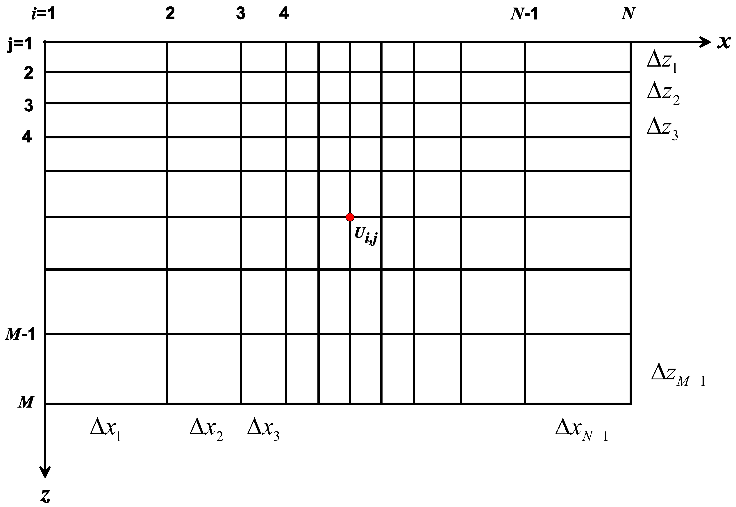
To solve the wavenumber domain electrical potential in Equation (5), we should divide the computational domain $\Omega$ into (N − 1) × (M − 1) rectangular elements, shown in Figure 2. The mesh is designed to be rectangular with an irregular grid spacing in the x-direction and z-direction. The nodes in the x-axis are represented by $i=1,2,3,\cdots ,N$, and the nodes in the z-axis are represented by $j=1,2,3,\cdots ,M$. The representative area $\Delta A$ for a source point in the interior can be written as

$$\Delta A=\frac{\left(\Delta x_i+\Delta x_{i-1}\right)\cdot \left(\Delta z_j+\Delta z_{j-1}\right)}{4},$$

and in the limit, at the ground surface with $z\to 0$,

$$\Delta A=\frac{\left(\Delta x_i+\Delta x_{i-1}\right)\cdot \Delta z_j}{4}.$$

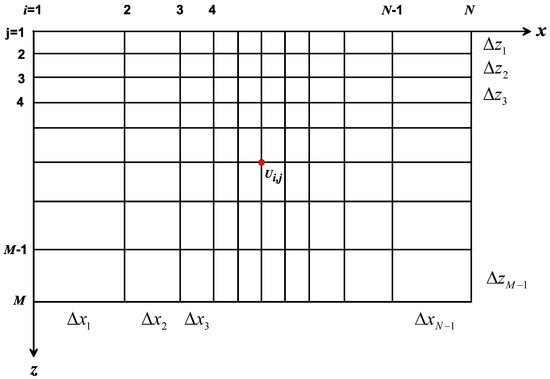
Figure 2. Discretization for two-dimensional geo-electric model.

.

3.1. Discretization of the Helmholtz Governing Equation

The 2D conductivity distribution $\sigma \left(x,z\right)$ is discretized at each node (i, j) by ${\sigma }_{i,j}$ and the wavenumber domain numerical solution $U_{i,j}$ at each node (i, j) needs to be calculated. At any interior node (i, j) with an irregular grid spacing in the x-axis and z-axis, the finite-difference approximation of second-order derivatives in Equation (5) can be written as

$$\begin{array}{ll}{\left[\frac{\partial }{\partial x}\left(\sigma \frac{\partial U}{\partial x}\right)\right]}_{i,j}& \approx \frac{1}{\frac{\Delta x_i+\Delta x_{i-1}}{2}}\left[{\left(\sigma \frac{\partial U}{\partial x}\right)}_{i+\frac{1}{2},j}-{\left(\sigma \frac{\partial U}{\partial x}\right)}_{i-\frac{1}{2},j}\right]\\ & \approx \frac{2}{\Delta x_i+\Delta x_{i-1}}\left[\frac{{\sigma }_{i+1,j}+{\sigma }_{i,j}}{2}\frac{U_{i+1,j}-U_{i,j}}{\Delta x_i}-\frac{{\sigma }_{i-1,j}+{\sigma }_{i,j}}{2}\frac{U_{i,j}-U_{i-1,j}}{\Delta x_{i-1}}\right]\\ & =\frac{{\sigma }_{i-1,j}+{\sigma }_{i,j}}{\left(\Delta x_i+\Delta x_{i-1}\right)\Delta x_{i-1}}{U}_{i-1,j}-\left[\frac{{\sigma }_{i-1,j}+{\sigma }_{i,j}}{\left(\Delta x_i+\Delta x_{i-1}\right)\Delta x_{i-1}}+\frac{{\sigma }_{i+1,j}+{\sigma }_{i,j}}{\left(\Delta x_i+\Delta x_{i-1}\right)\Delta x_i}\right]U_{i,j}\\ & \hspace{1em}+\frac{{\sigma }_{i+1,j}+{\sigma }_{i,j}}{\left(\Delta x_i+\Delta x_{i-1}\right)\Delta x_i}{U}_{i+1,j}\end{array},$$

(6)

and

$$\begin{array}{ll}{\left[\frac{\partial }{\partial z}\left(\sigma \frac{\partial U}{\partial z}\right)\right]}_{i,j}& \approx \frac{1}{\frac{\Delta z_j+\Delta z_{j-1}}{2}}\left[{\left(\sigma \frac{\partial U}{\partial z}\right)}_{i,j+\frac{1}{2}}-{\left(\sigma \frac{\partial U}{\partial z}\right)}_{i,j-\frac{1}{2}}\right]\\ & \approx \frac{2}{\Delta z_j+\Delta z_{j-1}}\left[\frac{{\sigma }_{i,j+1}+{\sigma }_{i,j}}{2}\frac{U_{i,j+1}-U_{i,j}}{\Delta z_j}-\frac{{\sigma }_{i,j-1}+{\sigma }_{i,j}}{2}\frac{U_{i,j}-U_{i,j-1}}{\Delta z_{j-1}}\right]\\ & =\frac{{\sigma }_{i,j-1}+{\sigma }_{i,j}}{\left(\Delta z_j+\Delta z_{j-1}\right)\Delta z_{j-1}}{U}_{i,j-1}-\left[\frac{{\sigma }_{i,j-1}+{\sigma }_{i,j}}{\left(\Delta z_j+\Delta z_{j-1}\right)\Delta z_{j-1}}+\frac{{\sigma }_{i,j+1}+{\sigma }_{i,j}}{\left(\Delta z_j+\Delta z_{j-1}\right)\Delta z_j}\right]U_{i,j}\\ & \hspace{1em}+\frac{{\sigma }_{i,j+1}+{\sigma }_{i,j}}{\left(\Delta z_j+\Delta z_{j-1}\right)\Delta z_j}{U}_{i,j+1}\end{array}.$$

(7)

Substituting Equations (6) and (7) into Equation (5), the finite-difference equation in the discretized form at any interior node can be written as follows:

$$\begin{array}{l}\frac{{\sigma }_{i-1,j}+{\sigma }_{i,j}}{\left(\Delta x_i+\Delta x_{i-1}\right)\Delta x_{i-1}}{U}_{i-1,j}+\frac{{\sigma }_{i+1,j}+{\sigma }_{i,j}}{\left(\Delta x_i+\Delta x_{i-1}\right)\Delta x_i}{U}_{i+1,j}\\ \hspace{1em}+\frac{{\sigma }_{i,j-1}+{\sigma }_{i,j}}{\left(\Delta z_j+\Delta z_{j-1}\right)\Delta z_{j-1}}{U}_{i,j-1}+\frac{{\sigma }_{i,j+1}+{\sigma }_{i,j}}{\left(\Delta z_j+\Delta z_{j-1}\right)\Delta z_j}{U}_{i,j+1}\\ \hspace{1em}\hspace{1em}-\left[\frac{{\sigma }_{i-1,j}+{\sigma }_{i,j}}{\left(\Delta x_i+\Delta x_{i-1}\right)\Delta x_{i-1}}+\frac{{\sigma }_{i+1,j}+{\sigma }_{i,j}}{\left(\Delta x_i+\Delta x_{i-1}\right)\Delta x_i}\right.\\ \hspace{1em}\hspace{1em}\hspace{1em}\left.+\frac{{\sigma }_{i,j-1}+{\sigma }_{i,j}}{\left(\Delta z_j+\Delta z_{j-1}\right)\Delta z_{j-1}}+\frac{{\sigma }_{i,j+1}+{\sigma }_{i,j}}{\left(\Delta z_j+\Delta z_{j-1}\right)\Delta z_j}+{\lambda }^2{\sigma }_{i,j}\right]U_{i,j}\\ \hspace{1em}\hspace{1em}\hspace{1em}\hspace{1em}=-Q\cdot \delta \left(x_s\right)\delta \left(z_s\right)\\ \end{array}.$$

(8)

Using scientific notation, Equation (8) can be written as

$$C_W^{ij}{U}_{i-1,j}+C_E^{ij}{U}_{i+1,j}+C_N^{ij}{U}_{i,j-1}+C_S^{ij}{U}_{i,j+1}+C_P^{ij}{U}_{i,j}=-Q\cdot \delta \left(x_s\right)\delta \left(z_s\right).$$

(9)

where $C_W^{ij}$ is the coupling coefficient related to the node (i − 1, j) and node (i, j), $C_E^{ij}$ is the coupling coefficient related to the node (i, j) and node (i + 1, j), $C_S^{ij}$ is the coupling coefficient related to the node (i, j − 1) and node (i, j), $C_S^{ij}$ is the coupling coefficient related to the node (i, j) and node (i, j + 1), and $C_P^{ij}$ is the self-coupling coefficient at node (i, j). All these coupling coefficients are given by

$$C_W^{ij}=\frac{{\sigma }_{i-1,j}+{\sigma }_{i,j}}{\left(\Delta x_i+\Delta x_{i-1}\right)\Delta x_{i-1}},$$

(10)

$$C_E^{ij}=\frac{{\sigma }_{i+1,j}+{\sigma }_{i,j}}{\left(\Delta x_i+\Delta x_{i-1}\right)\Delta x_i},$$

(11)

$$C_N^{ij}=\frac{{\sigma }_{i,j-1}+{\sigma }_{i,j}}{\left(\Delta z_j+\Delta z_{j-1}\right)\Delta z_{j-1}},$$

(12)

$$C_S^{ij}=\frac{{\sigma }_{i,j+1}+{\sigma }_{i,j}}{\left(\Delta z_j+\Delta z_{j-1}\right)\Delta z_j},$$

(13)

$$C_P^{ij}=-\left[C_W^{ij}+C_E^{ij}+C_N^{ij}+C_S^{ij}+{\lambda }^2{\sigma }_{i,j}\right].$$

(14)

3.2. Fictitious Point Technique for Boundary Conditions

3.2.1. Boundary Nodes Located on the Top Edge

For all top boundary nodes (i, j) with $i=2,3,\cdots ,N-1$ and j = 1, the boundary condition is of the homogeneous Neumann type $\frac{\partial U_{i,j}}{\partial n}=0$, i.e.,

$$U_{i,j-1}=U_{i,j+1}.$$

It can be implemented by assuming a fictitious row of nodes in the air at j = 0, such that the wavenumber domain electrical potential $U_{i,2}$ and the conductivity ${\sigma }_{i,2}$ at nodes (i, 2) are reflected at the imaginary nodes (i, 0). This fictitious point technique leads to the finite-difference form of Equation (5) given by

$$C_W^{ij}{U}_{i-1,j}+C_E^{ij}{U}_{i+1,j}+C_S^{ij}{U}_{i,j+1}+C_P^{ij}{U}_{i,j}=-Q\cdot \delta \left(x_s\right)\delta \left(z_s\right),$$

(15)

where the coupling coefficients are given by

$$C_W^{ij}=\frac{{\sigma }_{i-1,j}+{\sigma }_{i,j}}{\left(\Delta x_i+\Delta x_{i-1}\right)\Delta x_{i-1}},$$

(16)

$$C_E^{ij}=\frac{{\sigma }_{i+1,j}+{\sigma }_{i,j}}{\left(\Delta x_i+\Delta x_{i-1}\right)\Delta x_i},$$

(17)

$$C_S^{ij}=\frac{{\sigma }_{i,j+1}+{\sigma }_{i,j}}{{\left(\Delta z_j\right)}^2},$$

(18)

$$C_P^{ij}=-\left[C_W^{ij}+C_E^{ij}+C_S^{ij}+{\lambda }^2{\sigma }_{i,j}\right].$$

(19)

3.2.2. Boundary Nodes Located on the Bottom Edge

For all bottom boundary nodes (i, j) with $i=2,3,\cdots ,N-1$ and j = M, the homogeneous Neumann boundary condition $\frac{\partial U_{i,j}}{\partial n}=0$ can be written as

$$U_{i,j+1}=U_{i,j-1}.$$

Using the fictitious point technique, it will lead to the finite-difference form of Equation (5) given by

$$C_W^{ij}{U}_{i-1,j}+C_E^{ij}{U}_{i+1,j}+C_N^{ij}{U}_{i,j-1}+C_P^{ij}{U}_{i,j}=-Q\cdot \delta \left(x_s\right)\delta \left(z_s\right),$$

(20)

where the coupling coefficients are given by

$$C_W^{ij}=\frac{{\sigma }_{i-1,j}+{\sigma }_{i,j}}{\left(\Delta x_i+\Delta x_{i-1}\right)\Delta x_{i-1}},$$

(21)

$$C_E^{ij}=\frac{{\sigma }_{i+1,j}+{\sigma }_{i,j}}{\left(\Delta x_i+\Delta x_{i-1}\right)\Delta x_i},$$

(22)

$$C_N^{ij}=\frac{{\sigma }_{i,j-1}+{\sigma }_{i,j}}{{\left(\Delta z_{j-1}\right)}^2},$$

(23)

$$C_P^{ij}=-\left[C_W^{ij}+C_E^{ij}+C_N^{ij}+{\lambda }^2{\sigma }_{i,j}\right].$$

(24)

3.2.3. Boundary Nodes Located on the Left Edge

Using the fictitious point technique, the difference equation for boundary nodes (i, j) with $j=2,3,\cdots ,M-1$ and i = 1, has the form given as follows:

$$C_E^{ij}{U}_{i+1,j}+C_N^{ij}{U}_{i,j-1}+C_S^{ij}{U}_{i,j+1}+C_P^{ij}{U}_{i,j}=-Q\cdot \delta \left(x_s\right)\delta \left(z_s\right),$$

(25)

where the coupling coefficients are given by

$$C_E^{ij}=\frac{{\sigma }_{i+1,j}+{\sigma }_{i,j}}{{\left(\Delta x_i\right)}^2},$$

(26)

$$C_N^{ij}=\frac{{\sigma }_{i,j-1}+{\sigma }_{i,j}}{\left(\Delta z_j+\Delta z_{j-1}\right)\Delta z_{j-1}},$$

(27)

$$C_S^{ij}=\frac{{\sigma }_{i,j+1}+{\sigma }_{i,j}}{\left(\Delta z_j+\Delta z_{j-1}\right)\Delta z_j},$$

(28)

$$C_P^{ij}=-\left[C_E^{ij}+C_N^{ij}+C_S^{ij}+{\lambda }^2{\sigma }_{i,j}\right],$$

(29)

3.2.4. Boundary Nodes Located on the Right Edge

Using the fictitious point technique, the finite-difference equation for boundary nodes (i, j) with $j=2,3,\cdots ,M-1$ and i = N, has the form given as follows:

$$C_W^{ij}{U}_{i+1,j}+C_N^{ij}{U}_{i,j-1}+C_S^{ij}{U}_{i,j+1}+C_P^{ij}{U}_{i,j}=-Q\cdot \delta \left(x_s\right)\delta \left(z_s\right),$$

(30)

where the coupling coefficients are given by

$$C_W^{ij}=\frac{{\sigma }_{i-1,j}+{\sigma }_{i,j}}{{\left(\Delta x_{i-1}\right)}^2},$$

(31)

$$C_N^{ij}=\frac{{\sigma }_{i,j-1}+{\sigma }_{i,j}}{\left(\Delta z_j+\Delta z_{j-1}\right)\Delta z_{j-1}},$$

(32)

$$C_S^{ij}=\frac{{\sigma }_{i,j+1}+{\sigma }_{i,j}}{\left(\Delta z_j+\Delta z_{j-1}\right)\Delta z_j},$$

(33)

$$C_P^{ij}=-\left[C_W^{ij}+C_N^{ij}+C_S^{ij}+{\lambda }^2{\sigma }_{i,j}\right].$$

(34)

3.2.5. Corner Nodes with Fictitious Point Technique

For the top-left corner node (1, 1), the finite-difference equation can be written as

$$C_E^{ij}{U}_{i+1,j}+C_S^{ij}{U}_{i,j+1}+C_P^{ij}{U}_{i,j}=-Q\cdot \delta \left(x_s\right)\delta \left(z_s\right),$$

(35)

where $C_E^{ij}=\frac{{\sigma }_{i+1,j}+{\sigma }_{i,j}}{{\left(\Delta x_i\right)}^2}$, $C_S^{ij}=\frac{{\sigma }_{i,j+1}+{\sigma }_{i,j}}{{\left(\Delta z_j\right)}^2}$, and $C_P^{ij}=-\left[C_E^{ij}+C_S^{ij}+{\lambda }^2{\sigma }_{i,j}\right]$.

For the top-right corner node (N, 1), the finite-difference equation is

$$C_W^{ij}{U}_{i+1,j}+C_S^{ij}{U}_{i,j+1}+C_P^{ij}{U}_{i,j}=-Q\cdot \delta \left(x_s\right)\delta \left(z_s\right),$$

(36)

where $C_W^{ij}=\frac{{\sigma }_{i-1,j}+{\sigma }_{i,j}}{{\left(\Delta x_{i-1}\right)}^2}$, $C_S^{ij}=\frac{{\sigma }_{i,j+1}+{\sigma }_{i,j}}{{\left(\Delta z_j\right)}^2}$, and $C_P^{ij}=-\left[C_W^{ij}+C_S^{ij}+{\lambda }^2{\sigma }_{i,j}\right]$.

For the bottom-left corner node (1, M), the finite-difference equation is

$$C_E^{ij}{U}_{i+1,j}+C_N^{ij}{U}_{i,j+1}+C_P^{ij}{U}_{i,j}=-Q\cdot \delta \left(x_s\right)\delta \left(z_s\right),$$

(37)

where $C_E^{ij}=\frac{{\sigma }_{i+1,j}+{\sigma }_{i,j}}{{\left(\Delta x_i\right)}^2}$, $C_N^{ij}=\frac{{\sigma }_{i,j-1}+{\sigma }_{i,j}}{{\left(\Delta z_{j-1}\right)}^2}$, and $C_P^{ij}=-\left[C_E^{ij}+C_N^{ij}+{\lambda }^2{\sigma }_{i,j}\right]$.

For the bottom-right node (N, M), the finite-difference equation is

$$C_W^{ij}{U}_{i+1,j}+C_N^{ij}{U}_{i,j+1}+C_P^{ij}{U}_{i,j}=-Q\cdot \delta \left(x_s\right)\delta \left(z_s\right),$$

(38)

where $C_W^{ij}=\frac{{\sigma }_{i-1,j}+{\sigma }_{i,j}}{{\left(\Delta x_{i-1}\right)}^2}$, $C_N^{ij}=\frac{{\sigma }_{i,j-1}+{\sigma }_{i,j}}{{\left(\Delta z_{j-1}\right)}^2}$, and $C_P^{ij}=-\left[C_W^{ij}+C_N^{ij}+{\lambda }^2{\sigma }_{i,j}\right]$.

3.3. Solution of the Discrete Forward Equation System

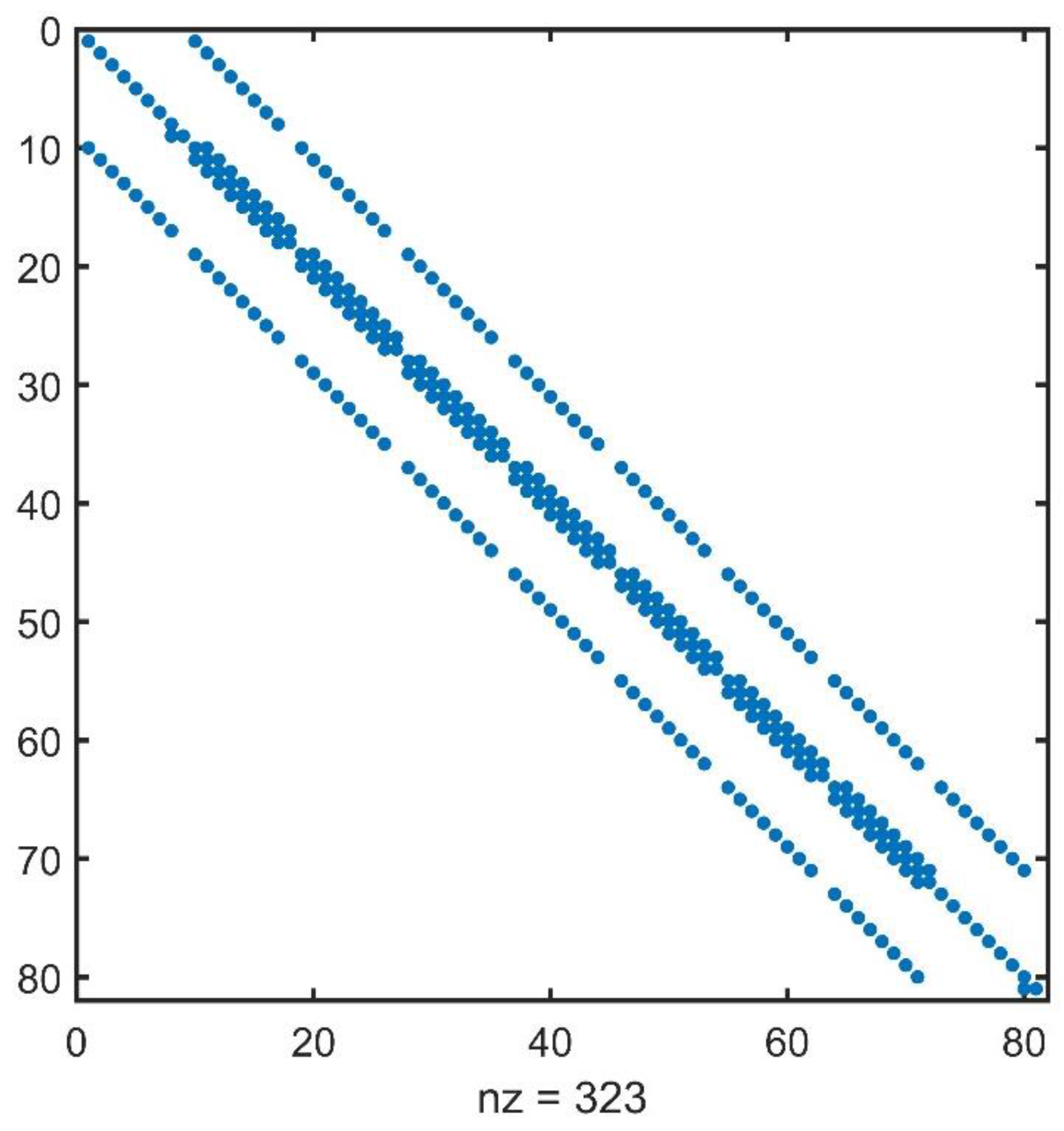
With the governing boundary value problem of Equation (5) being approximated using the finite-difference method in all N × M grid nodes, the linear algebraic equations (Equations (9), (15), (20), (25), (30) and (36)–(38)) must be properly arranged into a linear system as follows:

$$KU=p,$$

(39)

where $K$ is a matrix originating from the coupling coefficients, $U$ is the unknown wavenumber domain electrical potentials vector, and $p$ is the source vector containing $I/2\Delta A$ at the current electrode positions. The matrix $K$ generated by the finite-difference algorithm based on the fictitious point technique in Equation (39) can be a sparse, symmetric, and positive-definite matrix. Figure 3 shows the non-zero element distribution for an 8 × 8 grid (just for illustration purposes). Usually, Equation (39) can be considered an ill-conditioned problem. Therefore, the linear equation system generated by the finite-difference approximation for the wavenumber domain electrical potential can be solved by Krylov-type iterative methods. Meanwhile, the appropriate pre-conditioners can also significantly improve the speed of convergence. In forward modeling, the ILU-BICGSTAB iterative method is used, which combines a bi-conjugate gradient stabilization algorithm [29,30] with an incomplete LU decomposition [31].

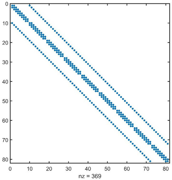
Figure 3. Nonzero element distribution of finite-difference coefficient matrix with an 8 × 8 grid.

For the numerical simulations of a simple 2D model, the discrete elements are designed as 100 × 100 in the whole computational domain and it takes 0.12 s by the ILU-BICGSTAB iterative method. Figure 4 shows the fast convergence curve and total number of the ILU-BICGSTAB iterative method. For multiple point sources, Equation (39) needs to be solved multiple times and the apparent resistivity needs to be calculated based on the corresponding observation device.

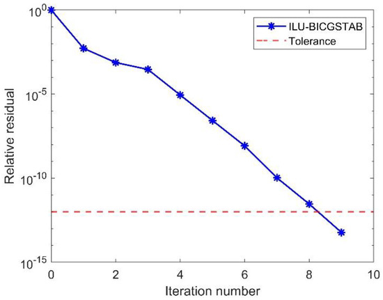
Figure 4. Convergence curve of the ILU-BICGSTAB iterative method with tolerance = 10⁻¹².

3.4. Calculation of Spatial-Domain Electrical Potential and Apparent Resistivity

After solving the discrete forward equation system, we can obtain the wavenumber domain electrical potentials $U\left(x,\lambda ,z\right)$ on each node, and then spatial-domain electrical potentials $u\left(x,y,z\right)$ can be calculated by the Fourier inverse transform. On the profile (y = 0), the Fourier inverse transform formula can be expressed as

$$u\left(x,0,z\right)=\frac{2}{\pi }{\displaystyle {\int }_0^{+\infty }U\left(x,\lambda ,z\right)\mathrm{d}\lambda }$$

(40)

Using numerical integration, Equation (40) can be rewritten as

$$u\left(r\right)\approx {\displaystyle \sum _{i=1}^N{g}_{i}U\left(r,{\lambda }_i\right)}$$

(41)

where N is the number of wavenumbers; $r=\sqrt{x^2+z^2}$ is the distance from the measured point on the profile to the source point; ${\lambda }_i$ are the discrete wavenumbers; and $g_i$ is the corresponding weighting coefficient. We use the optimization scheme developed by Xu et al. [32] to select the wavenumber. The wavenumber used in our 2.5D direct-current resistivity forward modeling is shown in Table 1.

Table 1. Discrete wavenumbers ${\lambda }_i$ and corresponding coefficients $g_i$ of inverse Fourier transform.

i	λi	gi
1	0.0066954	0.0099032
2	0.5160113	0.1759048
3	0.2388812	0.0760419
4	0.1295920	0.0578590
5	0.9918394	0.4483043
6	0.0623708	0.0292485
7	0.3515289	0.0678736
8	2.0863820	1.1451725
9	0.0282197	0.0170322
10	6.9549240	7.9501720

In direct-current resistivity exploration, a current source +I and a current sink −I are used to energize the conductive Earth, and the apparent resistivity can be defined as follows:

$${\rho }_s=G\frac{\Delta u}{I}$$

(42)

where G is a geometric factor, which depends upon the locations of electrodes, and $\Delta u$ is the electrical potential difference.

According to the above 2.5D finite-difference algorithm analysis, the complete workflow is shown in Figure 5, which can compute the approximate numerical electrical potential and apparent resistivity.

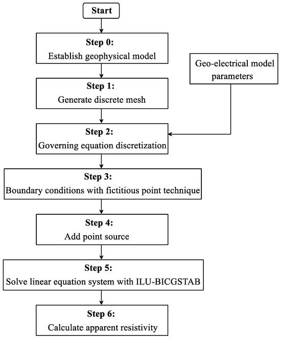
Figure 5. The main steps of 2.5D direct-current resistivity finite-difference forward algorithm based on fictitious point technique.

4. Numerical Experiments

The Lenovo Workstation P520 with an 8-Core Intel Xeon W-2145 processor including 32 GB of RAM was applied to execute our numerical simulation. The forward algorithm was developed in MATLAB (R2023a), and the subroutine is given in Appendix A.

4.1. Benchmark with Homogeneous Half-Space

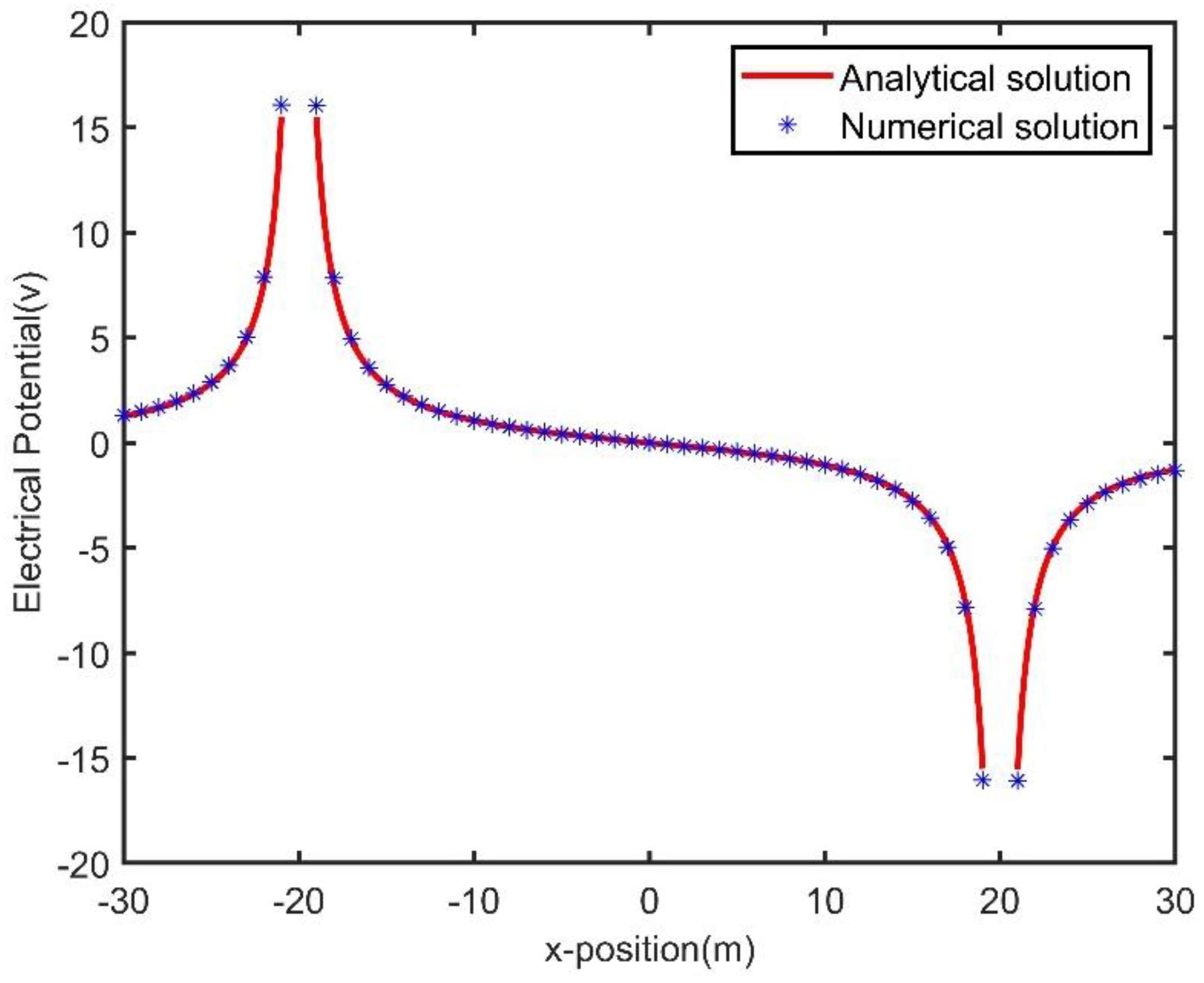
The benchmark of the accuracy of the finite-difference forward algorithm began with a homogeneous half-space model. The computational size was designed as 200 m × 100 m. The ground surface was considered flat and uniform, and homogeneous with a conductivity of 0.01 S/m. The positive and negative current electrode were placed at (−20 m, 0 m) and (20 m, 0 m), respectively, and the current was set as I = 1A. For the numerical simulation, we solved the problem on a 100 × 50 grid.

The numerical spatial-domain electrical potentials for the homogeneous half-space model are shown in Figure 6. It is evident that the spatial-domain electrical potentials computed by the finite-difference method with the fictitious point technique agree with the analytical solutions given in Appendix B. The finite-difference numerical results indicate that our fictitious point technique can provide high accuracy for 2.5D direct-current resistivity modeling.

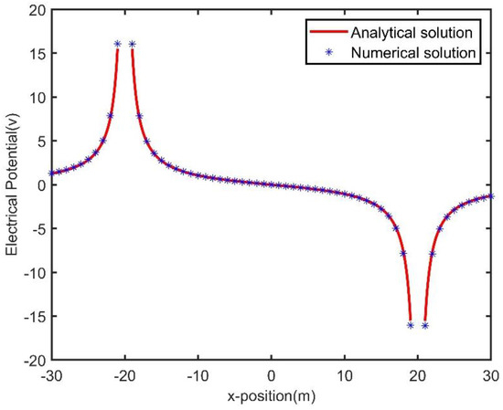
Figure 6. Comparison of analytical and finite-difference numerical solution of the point source potentials in the homogeneous half-space model.

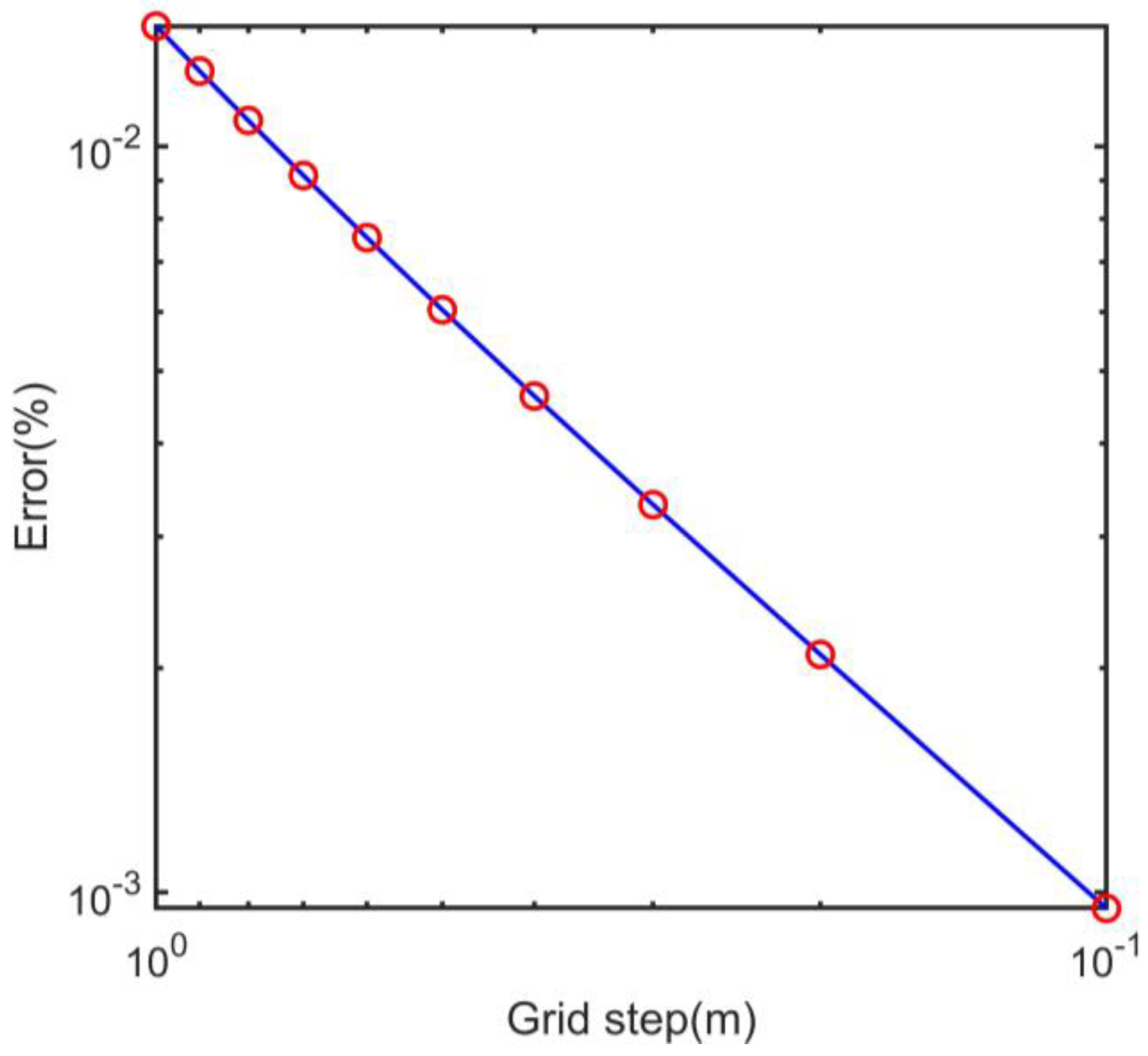
The relative root-mean-square error was used to measure the overall accuracy of our finite-difference scheme [33]:

$$\mathrm{Error}=\frac{\sqrt{{\displaystyle {\sum }_{i=1}^N{\displaystyle {\sum }_{j=1}^M{\left(u_{i,j}-{\tilde{u}}_{i,j}\right)}^2}}}}{\sqrt{{\displaystyle {\sum }_{i=1}^N{\displaystyle {\sum }_{j=1}^M{\left({\tilde{u}}_{i,j}\right)}^2}}}}\times 100\mathrm{per}\mathrm{cent},$$

(43)

where N and M are the numbers of observation nodes in the x- and y-direction, respectively, and $u_{i,j}$ and ${\tilde{u}}_{i,j}$ represent the numerical and analytical solution, respectively. Based on uniform meshes in the x-direction for the homogeneous half-space model, the convergence plot in the log–log scale for the relative root-mean-square error is shown in Figure 7. The error decreases as the grid step size becomes smaller, and numerical stability increases with respect to grid size. This further illustrates the accuracy of our finite-difference forward algorithm.

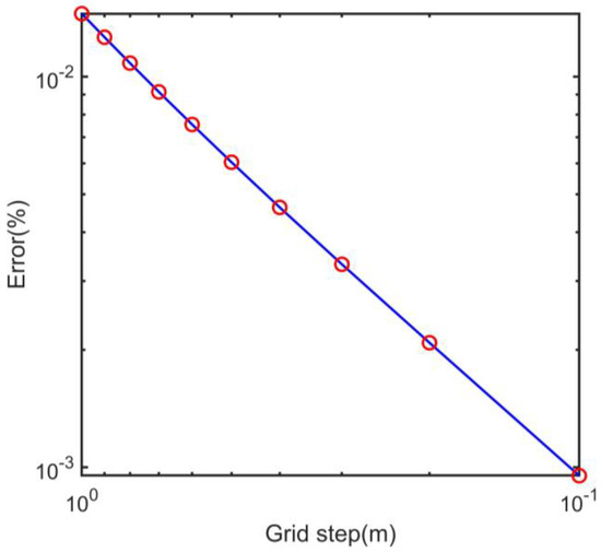
Figure 7. The convergence plot in log–log scale using relative root-mean-square error with step sizes in the interval [0.1, 1].

4.2. Two-Layer Conductivity Model

A two-layer conductivity model was applied for another numerical experiment to verify the accuracy of our forward modeling code. This two-layer model included a low-conductivity medium in the first layer and a high-conductivity medium in the second layer, as shown in Figure 8. The thickness of the low-conductivity medium was designed to be 4 m with a conductivity of 0.005 S/m, while the thickness of the high-conductivity medium was designed to be 100 m with a bearing conductivity of 0.05 S/m.

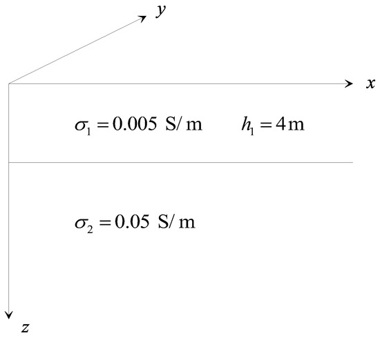
Figure 8. Schematic diagram of two-layered horizontal model.

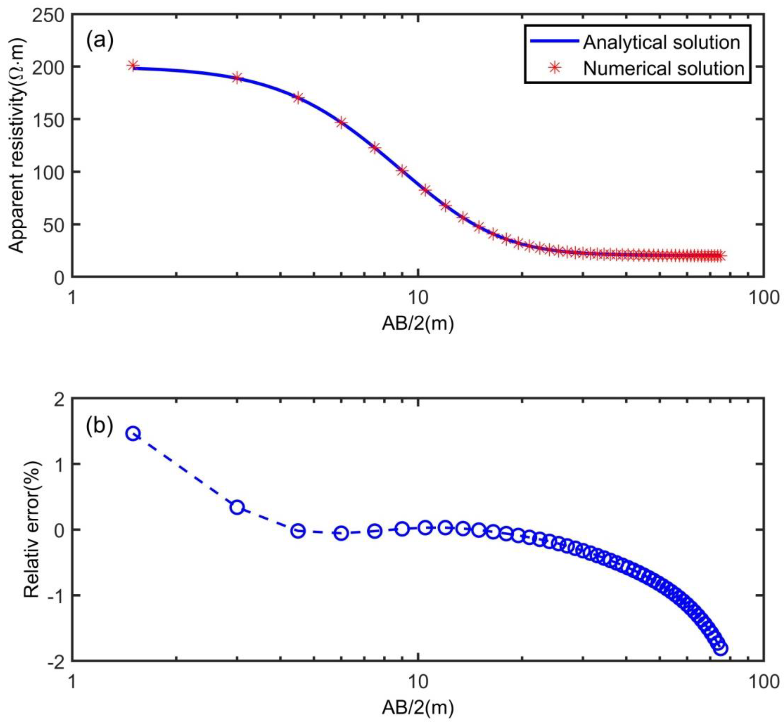
The computational domain was designed as 200 m × 200 m. The direct-current resistivity data were computed using the Wenner array by varying AB/2 from 1.5 m to 75 m, and the apparent resistivity curve calculated by the finite-difference scheme is displayed in Figure 9a. The finite-difference numerical results were compared to the analytical solutions given in Appendix C from Telford et al. [34]. The comparison between finite-difference numerical and analytical apparent resistivities shows a relative error below 2%, shown in Figure 9, which indicates that the 2.5D forward algorithm can satisfy practical requirements in terms of simulation accuracy. The maximum error occurs near the point source and AB/2 is approximately 70 m, but their relative errors are all within 2%. Further analysis shows that the errors in the 2.5D finite-difference forward modeling of direct-current sounding mainly come from three aspects: firstly, the errors are caused by singularity problems near the point source; secondly, the errors can be caused by truncating boundary conditions and finite-difference discretization; lastly, the errors are caused by numerical integration of the discrete Fourier inverse transform.

Figure 9. Comparison of analytical and finite-difference solutions for the two-layer resistivity model: (a) analytical and numerical values of apparent resistivity; (b) relative error.

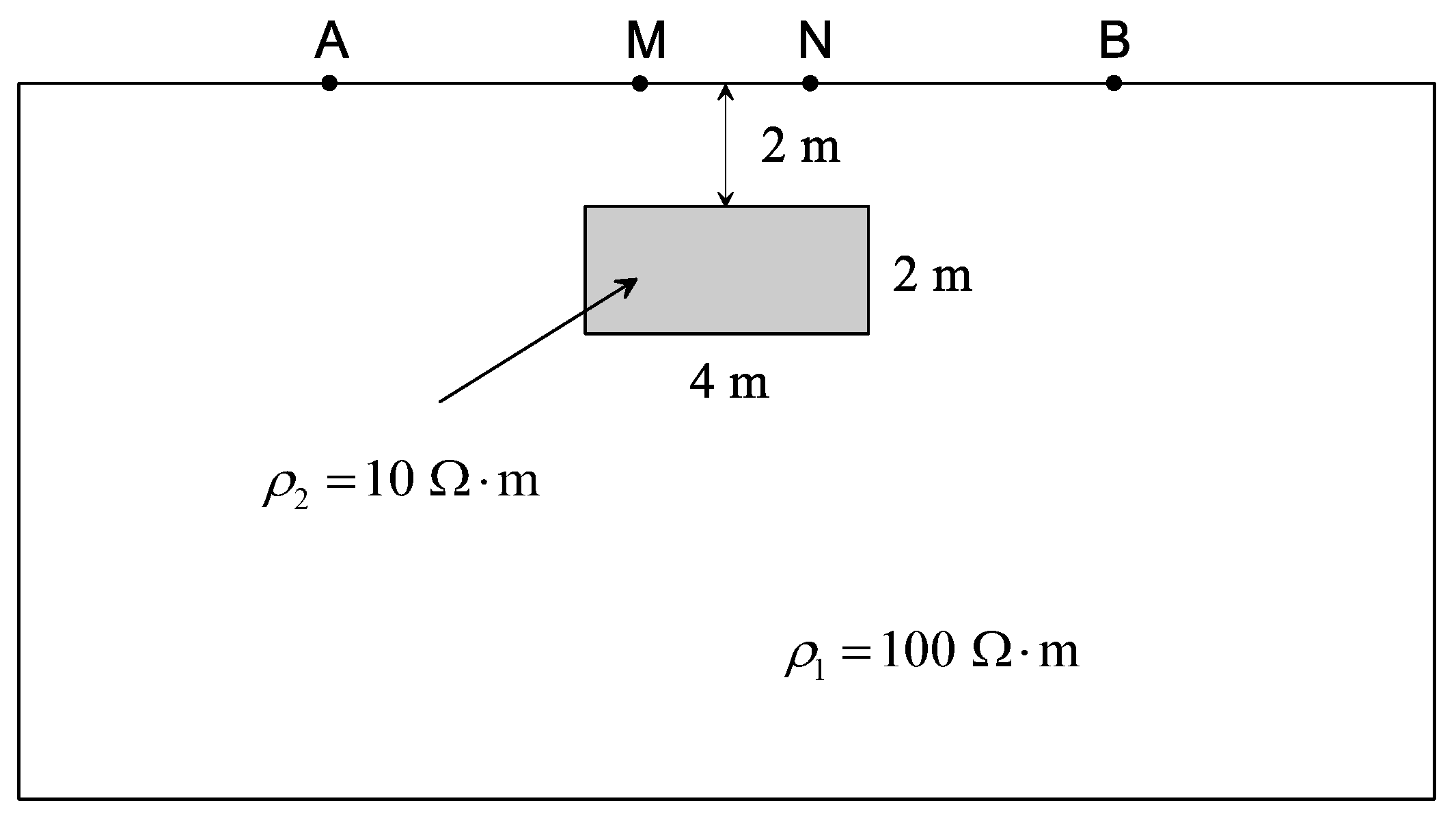
4.3. A Rectangular Conductive Body in Half-Space

To illustrate the accuracy and the efficiency of our finite-difference forward algorithm, the finite-element method with the structured rectangular mesh was adopted. In order to show a comparison of accuracy and efficiency, the numerical experiment was applied for a simple 2D model, which is shown in Figure 10. It was a symmetrical, rectangular, conductive body with a resistivity of 10 $\Omega \cdot \mathrm{m}$ inside a uniform half-space. The background resistivity of this 2D model was designed as 100 $\Omega \cdot \mathrm{m}$. The width and the thickness of the rectangular body were 4 m and 2 m, respectively. The rectangular body was located at a depth of 2 m from the ground surface.

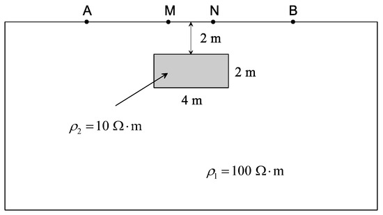
Figure 10. A two-dimensional geo-electrical model with rectangular body buried in the homogeneous half-space.

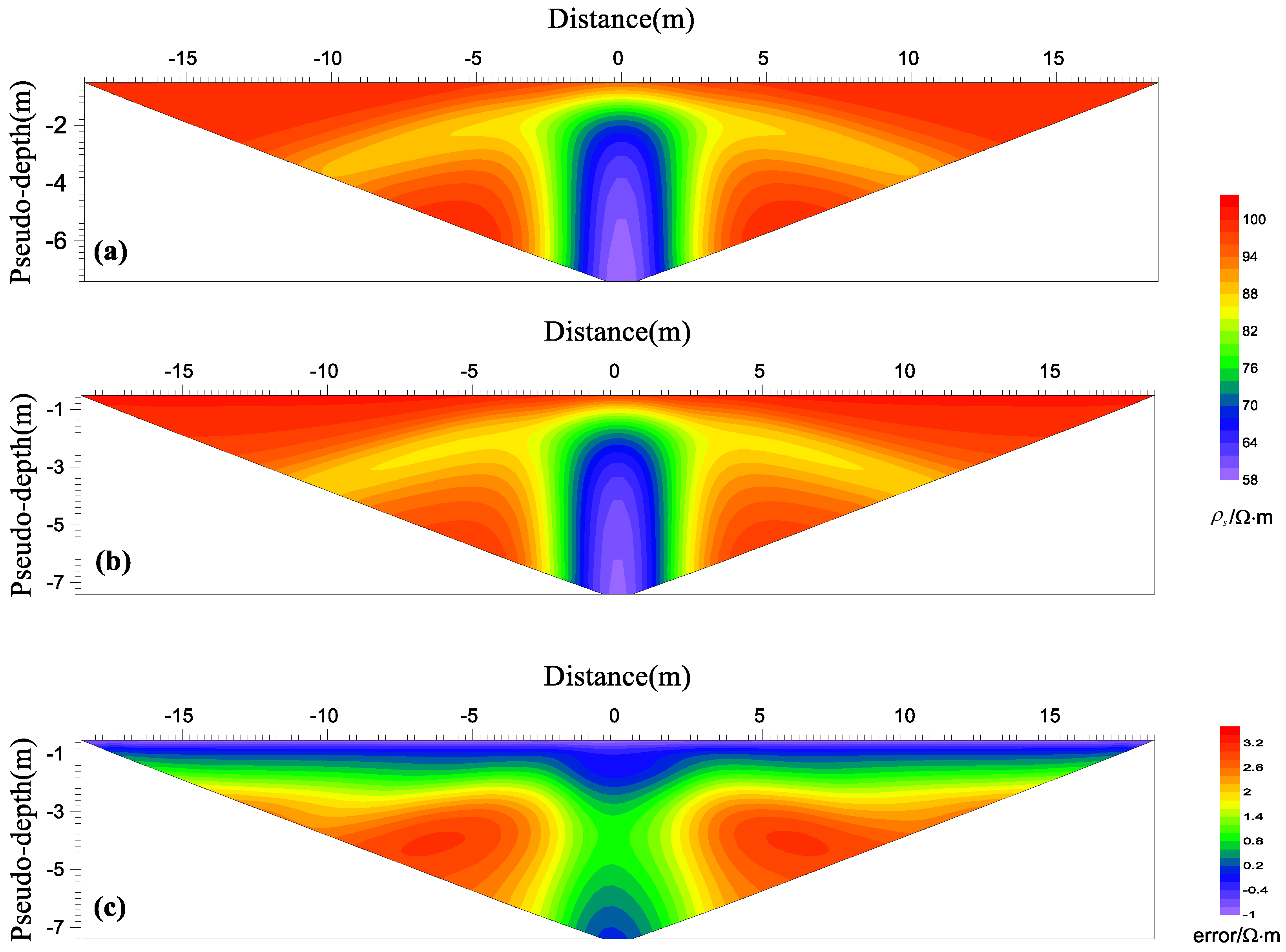
The computational size was designed as 100 m × 100 m. The Wenner-alpha array was selected for the simulation and the apparent resistivity pseudo-section calculated by finite-difference scheme is displayed in Figure 11a. In order to produce the closed contour map, the resistivity distribution characteristics of the low-resistivity anomalous body (or high-conductivity anomalous body) can be qualitatively distinguished, and the spatial distribution characteristics of the anomalous body can be accurately distinguished.

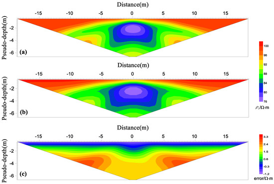
Figure 11. Numerical results for rectangular body model by different finite-element methods with Wenner-alpha electrode configuration: (a) finite-difference solution based on fictitious point technique; (b) finite-element solution based on Res2dmod software; (c) absolute error.

Figure 11b shows the apparent resistivity pseudo-section of the Wenner-alpha array calculated by the finite-element method from Res2dmod software (Windows version 3.03.06) [35]. The finite-difference results were compared to the finite-element solutions, and the absolute error is displayed in Figure 11c. The absolute errors are all within 4 $\Omega \cdot \mathrm{m}$. By comparing the finite-difference results with the fictitious point technique and the finite-element results, we found that the accuracy of the two ways is almost the same, and the results agree well.

If the Schlumberger array was selected to simulate the vertical electrical sounding data, the apparent resistivity pseudo-section calculated by finite-difference scheme is displayed in Figure 12a. As can be seen in Figure 12, the numerical apparent resistivities calculated by the finite-difference method with the fictitious point technique and the finite-element method with Res2dmod software are in close agreement with each other. Compared to the finite-element results (Figure 12b), the maximum absolute error for the apparent resistivity is 3.4 $\Omega \cdot \mathrm{m}$ (Figure 12c).

Figure 12. Numerical results for rectangular body model by different finite-element methods with Schlumberger electrode configuration: (a) finite-difference solution based on fictitious point technique; (b) finite-element solution based on Res2dmod software; (c) absolute error.

5. Discussion

In the finite-difference algorithm for 2.5D direct-current resistivity forward modeling, if the fictitious point technique was not applied, the coefficient matrix K in Equation (39) must be unsymmetrical and non-positive. Figure 13 shows the nonzero element distribution of a finite-difference coefficient matrix formed without a fictitious point technique based on an 8 × 8 grid (just for illustration purposes). The time consumption for solving the linear equation system of the finite-difference method without the fictitious point technique could be longer than that of the finite-difference method with the fictitious point approach.

Figure 13. Nonzero element distribution of finite-difference coefficient matrix formed without fictitious point technique based on an 8 × 8 grid.

Comparing the efficiency of two computing strategies, the homogeneous half-space model in Section 4.1 is adopted. The computational size is designed as 200 m × 100 m. The positive and negative current electrodes are placed at (−20 m, 0 m) and (20 m, 0 m), respectively, and the current is set as I = 1 A. The time consumption of the finite-difference method with the fictitious point technique is 0.12 s. However, the time consumption of the finite-difference method without the fictitious point technique is 0.65 s. The computational cost is mainly consumed for solving the linear equation system. In addition, the maximum relative error for the electrical potential using the fictitious point technique is 0.39%, and that without the fictitious point scheme is 31.56% (Figure 14). Therefore, the accuracy and efficiency of our 2.5D direct-current resistivity forward algorithm are superior to the finite-difference method without the fictitious point technique.

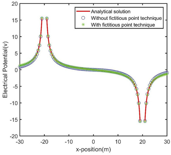
Figure 14. Comparison of numerical solution without fictitious point technique and numerical solution with fictitious point technique of the point source potentials in the homogeneous half-space model.

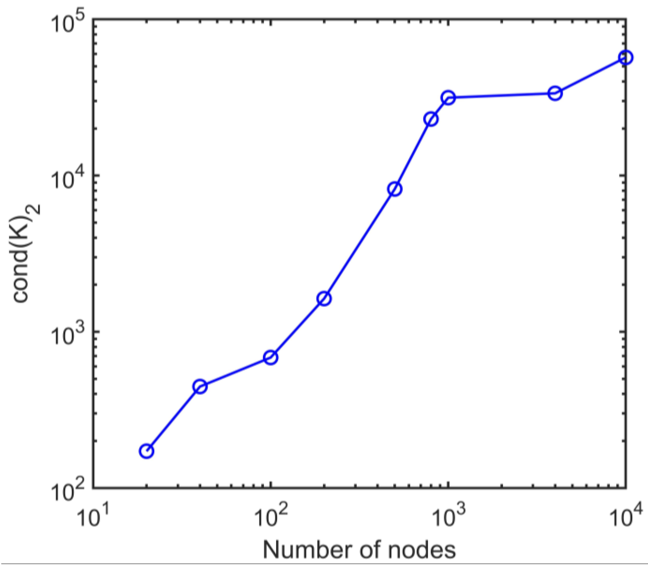
To discuss the stability of the proposed finite-difference scheme, let us also compute the condition number of the matrix K in Equation (39), since it turns out that this is a critical quantity in determining how rapidly certain iterative methods converge. The 2-norm condition number is defined by

$$cond{\left(K\right)}_2={‖K‖}_2{‖K^{-1}‖}_2=\sqrt{\frac{{\lambda }_{\max }\left(A^{T}A\right)}{{\lambda }_{\min }\left(A{A}^T\right)}},$$

(44)

where ${\lambda }_{\max }$ and ${\lambda }_{\min }$ are the maximum and minimum of the eigenvalues, respectively. The 2-norm condition number values as a function of the number of nodes for different meshes in the 2D wavenumber domain are shown in Figure 15. The fact that the matrix becomes more ill-conditioned as we refine the grid is responsible for the slow-down in the BICGSTAB iterative method.

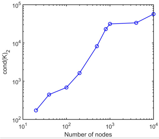
Figure 15. Condition number values as a function of the number of nodes for different meshes.

6. Conclusions

A high-accuracy 2.5D direct-current resistivity finite-difference forward algorithm based on a fictitious point technique is developed. We present the calculation formulas of this approach and provide a successful implementation. All mathematical formulas of the forward modeling algorithm are presented and implemented in MATLAB code. The numerical results show that the proposed algorithm has high accuracy for 2.5D direct-current resistivity forward modeling, which can provide a qualitative interpretation of field data.

Unlike the conventional finite-difference method without a fictitious point approach in the spatial domain, which can lead to a linear equation with an unsymmetrical and non-positive matrix, our scheme leads to a linear equation with a sparse, symmetrical positive matrix. Therefore, the computational time and the memory usage spent on solving the linear system equations should be lower than that of the conventional finite-difference method.

References

- Mosaad, A.H.; Farag, M.M.; Wei, Q.; Fahad, A.; Mohamed, S.A.; Hussein, A.S. Integration of electrical resistivity tomography and induced polarization for characterization and mapping of (Pb-Zn-Ag) sulfide deposits. Minerals 2023, 13, 986. [Google Scholar] [CrossRef]
- Mitchell, M.A.; Oldenburg, D.W. Using DC resistivity ring array surveys to resolve conductive structures around tunnels or mine-workings. J. Appl. Geophys. 2022, 211, 104949. [Google Scholar] [CrossRef]
- Oldenburg, D.W.; Li, Y.; Ellis, R.G. Inversion of geophysical data over a copper gold porphyry deposit: A case history for Mt. Milligan. Geophysics 1997, 62, 1419–1431. [Google Scholar] [CrossRef]
- Chambers, J.C.; Kuras, O.; Meldrum, P.I.; Ogilvy, R.D.; Hollands, J. Electrical resistivitytomography applied to geologic, hydrogeologic, and engineering investigations at a former waste-disposal site. Geophysics 2006, 71, 231–239. [Google Scholar] [CrossRef]
- Rucker, D.; Loke, M.H.; Levitt, M.T.; Noonan, G.E. Electrical resistivity characterization of an industrial site using long electrodes. Geophysics 2010, 75, 95–104. [Google Scholar] [CrossRef]
- Kim, J.H.; Tsourlos, P.; Karmis, P.; Vargemezis, G.; Yi, M.J. 3D inversion of irregular gridded 2D electrical resistivity tomography lines: Application to sinkhole mapping at the Island of Corfu (West Greece). Near Surf. Geophys. 2018, 14, 275–285. [Google Scholar] [CrossRef]
- Plank, Z.; Polgar, D. Application of the DC resistivity method in urban geological problems of karstic areas. Near Surf. Geophys. 2019, 17, 547–561. [Google Scholar] [CrossRef]
- Sirota, D.; Shragge, J.; Krahenbuhl, R.; Swidinsky, A.; Yalo, N.; Bradford, J. Development and validation of a low-cost direct current resistivity meter for humanitarian geophysics applications. Geophysics 2022, 87, 1–4. [Google Scholar] [CrossRef]
- Zhou, B.; Greenhalgh, M.; Greenhalgh, S.A. 2.5-D/3-D resistivity modelling in anisotropic media using Gaussian quadrature grids. Geophys. J. Int. 2009, 176, 63–80. [Google Scholar] [CrossRef]
- Zhang, H.; Liu, Y.; Yang, X. An efficient ADI difference scheme for the nonlocal evolution problem in three-dimensional space. J. Appl. Math. Comput. 2023, 69, 651–674. [Google Scholar] [CrossRef]
- Zhou, Z.; Zhang, H.; Yang, X. H1-norm error analysis of a robust ADI method on graded mesh for three-dimensional subdiffusion problems. Numer. Algorithms 2023, 94, 1–19. [Google Scholar] [CrossRef]
- Yang, X.; Wu, L.; Zhang, H. A space-time spectral order sinc-collocation method for the fourth-order nonlocal heat model arising in viscoelasticity. Appl. Math. Comput. 2023, 457, 128192. [Google Scholar] [CrossRef]
- Tian, Q.; Yang, X.; Zhang, H.; Xu, D. An implicit robust numerical scheme with graded meshes for the modified Burgers model with nonlocal dynamic properties. Comput. Appl. Math. 2023, 42, 246. [Google Scholar] [CrossRef]
- Mufti, I.R. Finite-difference resistivity modeling for arbitrarily shaped two-dimensional structures. Geophysics 1976, 41, 62–78. [Google Scholar] [CrossRef]
- Vachiratienchai, C.; Boonchaisuk, S.; Siripunvaraporn, W. A hybrid finite difference-finite element method to incorporate topography for 2D direct current (DC) resistivity modeling. Phys. Earth Planet. Interiors 2010, 183, 426–434. [Google Scholar] [CrossRef]
- Gernez, S.; Bouchedda, A.; Gloaguen, E.; Paradis, D. AIM4RES, an open-source 2.5D finite difference MATLAB library for anisotropic electrical resistivity modeling. Comput. Geosci. 2020, 135, 104401. [Google Scholar] [CrossRef]
- Jahandari, H.; Lelièvre, P.; Farquharson, C.G. Forward modeling of direct-current resistivity data on unstructured grids using an adaptive mimetic finite-difference method. Geophysics 2023, 88, 123–134. [Google Scholar] [CrossRef]
- Suryavanshi, D.; Dehiya, R. A mimetic finite-difference method for two-dimensional DC resistivity modeling. Math. Geosci. 2023, 55, 1189–1216. [Google Scholar] [CrossRef]
- Zhou, B.; Greenhalgh, S.A. Finite element three-dimensional direct current resistivity modelling: Accuracy and efficiency considerations. Geophys. J. Int. 2001, 145, 679–688. [Google Scholar] [CrossRef]
- Pan, K.J.; Tang, J. 2.5-D and 3-D DC resistivity modelling using an extrapolation cascadic multigrid method. Geophys. J. Int. 2014, 197, 1459–1470. [Google Scholar] [CrossRef]
- Chou, T.K.; Chouteau, M.; Dubé, J.S. Intelligent meshing technique for 2D resistivity inverse problems. Geophysics 2016, 81, 45–56. [Google Scholar] [CrossRef]
- Yan, B.; Li, Y.; Liu, Y. Adaptive finite element modeling of direct current resistivity in 2-D generally anisotropic structures. J. Appl. Geophys. 2016, 130, 169–176. [Google Scholar] [CrossRef]
- Ren, Z.Y.; Qiu, L.; Tang, J. 3D direct current resistivity anisotropic modelling by goal-oriented adaptive finite element methods. Geophys. J. Int. 2018, 212, 76–87. [Google Scholar] [CrossRef]
- Doyoro, Y.G.; Chang, P.Y.; Puntu, J.M.; Puntu, J.M.; Lin, D.J.; Huu, T.V.; Rahmalia, D.A.; Shie, M.S. A review of open software resources in python for electrical resistivity modelling. Geosci. Lett. 2022, 9, 3. [Google Scholar] [CrossRef]
- Pidlisecky, A.; Knight, R. FW2_5D: A MATLAB 2.5-D electrical resistivity modelling code. Comput. Geosci. 2008, 34, 1645–1654. [Google Scholar] [CrossRef]
- Ma, C.; Liu, J.; Liu, H.; Guo, R.; Musa, B.; Cui, Y. 2.5D electric resistivity forward modeling with element-free Galerkin method. J. Appl. Geophys. 2019, 162, 47–57. [Google Scholar] [CrossRef]
- Xu, S.Z.; Zhou, H. Modelling the 2D terrain effect on MT by the boundary-element method. Geophys. Prospect. 1997, 45, 931–943. [Google Scholar] [CrossRef]
- Dey, A.; Morrisson, H.F. Resistivity modeling for arbitrarily shaped three-dimensional structures. Geophysics 1979, 44, 753–780. [Google Scholar] [CrossRef]
- Liu, J.; Liu, P.; Tong, X. Three-dimensional land FD-CSEM forward modeling using edge finite-element method. J. Cent. South Univ. 2018, 25, 131–140. [Google Scholar] [CrossRef]
- Chen, J.; Haber, E.; Oldenburg, D.W. Three-dimensional numerical modelling and inversion of magnetometric resistivity data. Geophys. J. Int. 2002, 149, 679–697. [Google Scholar] [CrossRef]
- Pan, K.; Wang, J.; Hu, S.; Ren, Z.; Cui, T.; Guo, R.; Tang, J. An efficient cascadic multigrid solver for 3-D magnetotelluric forward modelling problems using potentials. Geophys. J. Int. 2022, 230, 1834–1851. [Google Scholar] [CrossRef]
- Xu, S.Z.; Duan, B.C.; Zhang, D.H. Selection of the wavenumbers k using an optimization method for the inverse Fourier transform in 2.5D electrical modeling. Geophys. Prospect. 2000, 48, 789–796. [Google Scholar] [CrossRef]
- Pan, K.; Zhang, Z.; Hu, S.; Ren, Z.; Guo, R.; Tang, J. Three-dimensional forward modelling of gravity field vector and its gradient tensor using the compact difference schemes. Geophys. J. Int. 2021, 224, 1272–1286. [Google Scholar] [CrossRef]
- Telford, W.M.; Geldart, L.P.; Sheriff, R.E. Applied Geophysics; Cambridge University Press: Cambridge, UK, 1990. [Google Scholar]
- Loke, M.H.; Barker, R.D. Rapid least-squares inversion of apparent resistivity pseudosections by a quasi-Newton method. Geophys. Prospect. 1996, 44, 131–152. [Google Scholar] [CrossRef]
Disclaimer/Publisher’s Note: The statements, opinions and data contained in all publications are solely those of the individual author(s) and contributor(s) and not of MDPI and/or the editor(s). MDPI and/or the editor(s) disclaim responsibility for any injury to people or property resulting from any ideas, methods, instructions or products referred to in the content. |
© 2024 by the authors. Licensee MDPI, Basel, Switzerland. This article is an open access article distributed under the terms and conditions of the Creative Commons Attribution (CC BY) license (https://creativecommons.org/licenses/by/4.0/).