Abstract
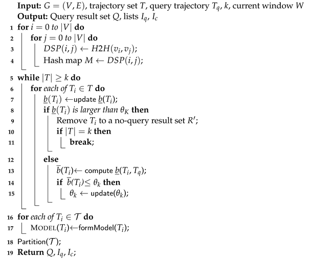
Continuous k-similarity trajectories search over a data stream is an important problem in the domain of spatio-temporal databases. Given a set of trajectories and a query trajectory over road network , the system monitors trajectories within , reporting k trajectories that are the most similar to whenever one time unit is passed. Some existing works study k-similarity trajectories search over trajectory data, but they cannot work in a road network environment, especially when the trajectory set scale is large. In this paper, we propose a novel framework named RNDLP (Road Network-based Distance Lower-bound-based Prediction) to support CKTRN over trajectory data. It is a distributed framework based on the following observation. That is, given a trajectory and the query trajectory , when we have knowledge of D(), we can compute the lower-bound and upper-bound distances between and , which enables us to predict the scores of trajectories in and employ these predictions to assess the significance of trajectories within . Accordingly, we can form a mathematical model to evaluate the excepted running cost of each trajectory we should spend. Based on the model, we propose a partition algorithm to partition trajectories into a group of servers so as to guarantee that the workload of each server is as the same as possible. In each server, we propose a pair-based algorithm to predict the earliest time could become a query result, and use the predicted result to organize these trajectories. Our proposed algorithm helps us support query processing via accessing a few points of a small number of trajectories whenever trajectories are updated. Finally, we conduct extensive performance studies on large, real, and synthetic datasets, which demonstrate that our new framework could efficiently support CKST over a data stream.
MSC:
68P20
1. Introduction
This paper addresses the challenge of continuous k-similarity trajectories (abbreviated as CKTRN) search over road networks, a problem with various applications [1,2,3,4,5]. Notably, CKTRN finds applications in diverse domains [6,7,8,9]. For instance, it proves beneficial in identifying compressed representations of trajectories while preserving their essential characteristics, leading to reduced storage requirements and transmission costs. Moreover, CKTRN plays a pivotal role in traffic analysis by uncovering trajectories with consistent patterns and behaviors. This information is valuable for predicting congestion, understanding traffic flow, and optimizing road networks. Lastly, it facilitates the clustering and grouping of moving objects exhibiting similar movement patterns, providing insights for urban planning, traffic analysis, and beyond.
Let represent the road network with V being the vertex set and E the edge set [1,10]. Each edge e is represented by the tuple , where and denote the starting and ending points of the edge e, respectively, and w refers to the weight of e, which equals the distance between and within G. Consequently, the trajectory of a moving object o across G is defined as the tuple . This includes a collection of n points generated by o over the last n time units. Each point within G is represented as , referring to the fact that p is positioned on edge e, arriving at vertex v after covering a distance of d. In this paper, points in P are modeled by a time-based window [11]. Under this setting, points are generated during the last n time unit. Whenever one time unit is passed, the first point could be regarded as an expired point, and we remove it from P. A newly generated point is inserted into P.
Let represent a query trajectory [1,2,12], which monitors a set of trajectories denoted as . Whenever one time unit is passed, it performs a search among the trajectories in and returns the k trajectories with the lowest scores to the system. In this context, the score of a trajectory , denoted as D(), is determined by the distance between and the query trajectory . Given a trajectory and a query trajectory , the distance between the corresponding point and is defined as the shortest distance between these points within the road network G. The distance between trajectory T and query trajectory is calculated as the sum of distances among their corresponding points.
Take an example in Figure 1a. There are three trajectories contained in . Each trajectory contains four GPS points generated by the moving object during the last four time units, i.e., contains four GPS points generated by the moving object , which are . is the query trajectory, refers to the fact that is the first GPS point of trajectory and is positioned on edge , arriving at vertex after covering a distance of 100 m. Assume that the moving objects can travel up to 100 m per time unit. The distance between and equals 1600 (=100 + 300 + 500 + 700). The distances among and these three trajectories are , respectively. As , the query result is . As shown in Figure 1b, after one time unit is passed, points in are updated to , the distance between and these three trajectories are updated to , respectively, and the query results are updated to .
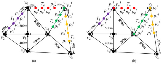
Figure 1.
Continuous k-similarity trajectory search over road network (), where (a) denotes the initial case of a given trajectory; (b) denotes the update of the trajectory and query results after one unit of time has elapsed.
This approach also holds significant practical applications. For instance, it can play a crucial role in a real-time anti-tracking system. Specifically, a user u might submit a request to the system to check if there are any existing trajectories tracking u. The system can fulfill this request by identifying k trajectories that are most similar to the real-time trajectory generated by u. If certain trajectories closely resemble this trajectory, it suggests potential tracking of u, and the system can promptly relay this information to u. Additionally, CKST has the potential for extensions into other real-time systems such as online car sharing [13], popular route identification, and more.
Numerous researchers have studied the problem of k-similarity trajectories search [14,15,16,17,18]. However, a major portion of these endeavors have primarily concentrated on addressing k-similarity trajectories search over static or historical trajectory datasets. Sacharidis et al. [13] explored the CKTRN problem within the context of data streams, enabling the retrieval of similar trajectories in real time. Yet, their approach measures similarity by considering the distance between two representative points corresponding to these trajectories (as discussed in Section 2). This method often fails to accurately evaluate trajectory similarity in various scenarios. Another effort proposed by Zhu et al. [19] investigated CKTRN over GPS point-based data streams. However, the similarity between two trajectories is measured based on the Euclidean distance among the corresponding GPS points, which cannot effectively work under a road network. Therefore, an efficient algorithm that could both accurately evaluate similarity among trajectories and support CKTRN in real time is desired.
However, efficiently supporting CKTRN over a road network poses several challenges. Firstly, the scale of each trajectory is typically large. In the context of data streams, where trajectory points are frequently updated, efficiently updating trajectory scores in real time becomes a challenging task. Secondly, the trajectory set scale is also extensive. As the window slides (with each time unit passing), updating scores for all trajectories and efficiently identifying new query result trajectories from a large set of trajectories involve a substantial computational cost. Moreover, maintaining all trajectories in a single server is challenging. Thirdly, in the context of road network environments, the computational overhead involved in calculating the distance between two points introduces its own set of challenges, further escalating the overall computational cost.
In this paper, we introduce a novel framework called RNDLP (Road Network-based Distance Lower-bound-based Prediction) designed to support CKTRN over road networks. This framework is distributed and relies on two key observations. Firstly, considering a road network , both edges and vertices in E and V do not frequently update. Consequently, we can pre-calculate the shortest distances among all vertices in G and employ these pre-computed values to streamline distance calculations among trajectory points.
Secondly, considering a non-query result trajectory and the query trajectory , when we have knowledge of D(), we can compute the lower-bound and upper-bound distances between and . This computation enables us to predict the scores of trajectories in and use these predictions to assess the significance of trajectories within . Essentially, if the lower-bound score of remains consistently high over numerous time units, it indicates that this trajectory is not likely to become a query result for an extended period. As a result, such a trajectory holds lower importance, and there is no need to closely monitor it over the long term. Conversely, trajectories with fluctuating scores require more frequent monitoring. In essence, only a small subset of trajectories needs score tracking with each passing time unit. In summary, our contributions can be outlined as follows.
- Hash-based Distance Calculation. We introduce a hash-based index to manage distances between points within the road network G. Specifically, we pre-compute the distances between vertices using the Floyd algorithm and use a hash table to maintain distance among any two vertices. In this way, we need not to spend high running costs in calculating the distance between two points. Alternatively, we can use running cost in computing the distance between two GPS points over a road network.
- Pair-based Dynamic Prediction Algorithm. We introduce a novel algorithm called PAIRDP (short for PAIR-based Dynamic Prediction) as an enhancement of the PDSP algorithm discussed in [20]. PAIRDP brings improvements in two main aspects. Firstly, it harnesses the inherent spatiotemporal correlation in GPS points to improve the accuracy of predicting the optimal moment for trajectories to potentially become query results. This correlation contributes to refining the prediction process and achieving more precise results. Secondly, PAIRDP incorporates a dynamic adjustment mechanism for predicting the moments when trajectories could potentially become query results. This adjustment relies on the scores of the query result trajectories. By integrating this dynamic adjustment, the algorithm can significantly reduce the frequency of trajectory access, resulting in improved operational efficiency.
- Model-based Partition Algorithm. Utilizing the prediction results, we can establish a cost model to assess the anticipated running cost of each trajectory. Consequently, we introduce a greedy algorithm to partition trajectories into different servers, ensuring that the workload of each server is as evenly distributed as possible. Additionally, we propose an incremental maintenance algorithm to adapt the partition under a data stream.
The remainder of this paper is structured as follows. Section 2 provides an overview of the existing literature in the field and outlines the problem definition. Section 3 introduces our proposed framework. In Section 4, we present the outcomes of our comprehensive experimental evaluation. Lastly, Section 5 offers concluding remarks by summarizing our key findings.
2. Preliminary
In this section, we will first review some important existing results related to k-similarity trajectory search. We will then introduce the problem definition.
2.1. Related Works
In recent years, researchers have focused on addressing the challenge of trajectory similarity search [8,10,21]. The endeavors in this domain can be categorized into two parts: ad hoc k-similarity trajectories queries and continuous k-similarity trajectories queries. Ad hoc k-similarity trajectory queries concentrating on enhancing query result accuracy through the design of similarity functions. For example, Lei Chen et al. [22] devised the EDR (Edit Distance on Real sequence) similarity measure function. Gajanan Gawde [23] leveraged trajectory polygon shapes for similarity comparisons.
The continuous k-similarity trajectories query can be further categorized into historical trajectory data-based and streaming trajectory data-based methods. Historical trajectory data-based approaches, exemplified by Güting et al. [20], utilize spatio-temporal indexes like R-trees to support query processing. They consider each trajectory as a sequence of units, constructing an index structure to facilitate a k-nearest neighbor search. On the other hand, streaming trajectory data-based methodologies, as studied by Sacharidis et al. [13], handle the continuous updating of trajectory data. These methods evaluate the distance between a query object and other mobile objects within a time window based on their maximum or minimum distance over timestamps. However, this approach utilizes only a subset of GPS points to represent trajectory distances, potentially affecting query precision.
Zhu et al. [19] proposed a sketch-based prediction algorithm to support a GPS point-based k-similarity trajectories search. The algorithm is based on the following observation. That is, if the distance between the last points of the query trajectory, denoted as , and the corresponding point in a trajectory is large, the overall distance of to , denoted as D(), will also be large. The authors provide formal bounds for the upper bound (()) and lower bound (()) of based on this observation. In addition to the score bounds calculation, Zhu et al. propose a structure called Partition-based Distance Sketch (PDS). The PDS is designed to summarize the distance distribution among GPS points in each trajectory and the query trajectory . It provides a compact representation of the distances between points within each trajectory, enabling efficient prediction and query result determination. Using the PDS, the algorithm can avoid continuously monitoring every trajectory until their predicted moments (). Consequently, it can save lots of running costs, and the corresponding GPS points generated within the time interval can be safely deleted, further reducing the storage requirements.
Discussion. In summary, most algorithms are based on the historical trajectory database, which cannot support query processing in real time. The algorithm proposed by Dimitris et al. cannot accurately evaluate similarity among trajectories in many cases. The effort proposed by Zhu et al. is based on GPS points. Therefore, an efficient algorithm that could both accurately evaluate similarity among trajectories and support the k-similar trajectories search in real time is desired.
2.2. Problem Definition
A time-based [24] window can be formally defined as a data organization and management technique that partitions a continuous stream of data into fixed or variable time intervals. Formally, a time-based window can be represented as a tuple , where T represents the current timestamp or time reference point. denotes the duration or length of the time interval, which defines the size of the window. In this paper, we apply time-based sliding windows to model trajectory data over road network as stated in Definition 1.
Definition 1 (Trajectory under Sliding Window).
A trajectory T of an object o, represented by the tuple , contains a group of GPS points traversing the road network G, generated within the last time units.
To be more specific, let be a trajectory within the trajectory set . can be denoted as , respectively. With the passage of each time unit, a point is removed from and another point is inserted into it. Each GPS point p in is defined as , indicating that p resides on edge e and arrives at vertex v with a distance of d.
The distance between two trajectories, T and , is calculated using Equation (1). Here, represents the distance between two GPS points and contained in T and , respectively. This distance corresponds to the shortest distance between and across the road network G. (or ) signifies the i-th generated GPS point in T (or ).
Take an example in Figure 1. Let be the trajectory of an object at the time unit . It contains the set of the last four GPS points generated by . After one time unit is passed, is removed from , and is inserted into . In other words, is updated to at . The distance between and equals 100, and D() is 1600 m at . After one time unit, is removed from , and is inserted . D() is updated to 2300 m. In the following, we will formally introduce the problem definition.
Definition 2 (CKTRN).
Let represent a set of N trajectories over road network G. We consider a query with being the query trajectory and k being a query parameter. The objective of a CKTRN is to monitor these N trajectories, and return k trajectories with the smallest scores to the system whenever one time unit is passed.
Back to the example in Figure 1. At , the distances between and these 3 trajectories are , respectively. As , the query result is . After one time unit is passed, the distances between and these three trajectories are updated to . The query result is updated to .
In essence, the CKST identifies the k trajectories with the smallest scores and presents them as the top-k most similar trajectories to the query trajectory . This process is performed periodically to ensure continuous monitoring and retrieval of the most similar trajectories over time. In this context, the score of each trajectory , denoted as D(), is determined by the distance between and the query trajectory . The CKST constantly computes and updates these scores based on the evolving positions of the trajectories in real time.
3. The Framework RNDLP
In this section, we introduce a novel framework called RNDLP (Road Network-based Distance Lower-bound-based Prediction) to address CKTRN over road networks. The structure of this section is organized as follows: we provide an overview of the framework initially. Subsequently, we detail the approach used to calculate distances among GPS points over road networks. Thirdly, we explain the partition-based initiation algorithm. Last in this section is the incremental maintenance algorithm.
3.1. The Framework Overview
Let represent the road network. The RNDLP framework initiates by pre-processing the road network, calculating the shortest paths between any pair of vertices in the vertex set V (Algorithm 1). This pre-processing involves constructing a hash table H to store the shortest path lengths between each vertex pair in V (lines 1–4). The construction process of this hash table will be explained in Section 3.2.
| Algorithm 1: The Framework Overview |
 |
After construction, the RNDLP framework scans each trajectory, calculates the lower-bound and upper-bound distances among each trajectory in the trajectory set and the query trajectory (lines 5–15). More precisely, an initial set R is formed, containing all trajectories. Then, for each trajectory , if the lower bound is greater than a threshold , it signifies that cannot become a temporary query result trajectory at the current moment. In this scenario, is removed from the set R to another set . Here, the threshold corresponds to the k-th lowest score among all trajectories in , and the manner of calculating and will be explained in the later section.
The aforementioned operations are iteratively executed until the number of trajectories in the set R is reduced to k. At this stage, the remaining k trajectories in set R are deemed the query result trajectories. Additionally, the framework predicts the moment when each trajectory has the potential to become a query result trajectory. In this paper, we introduce a pair-based algorithm to calculate and for each , with a detailed explanation provided in Section 3.3. The prediction algorithm will be discussed in Section 3.4.
Intuitively, the earlier the prediction moment of a trajectory, the more crucial it is to the query trajectory, and the higher the running cost it incurs. To ensure the workload (or communication cost) of each server is as evenly distributed as possible, we construct a cost model based on the lower-bound score of each trajectory. We form this model to assess the running cost associated with each trajectory. Utilizing this model, we can allocate trajectories based on their expected running cost, thereby minimizing the workload differences among different servers. Additionally, we present a greedy algorithm to partition trajectories in among a group of servers. The cost model and partition algorithm will be elaborated upon in Section 3.5 (lines 19–20).
Once sets R and the partition are formed, the incremental algorithm is executed. In comparison to the algorithm discussed in previous work, our proposed algorithm can dynamically adjust the threshold value . This dynamic adjustment aids in reducing the frequency of score calculations for trajectories in . In addition, we should dynamically adjust the partition. Comprehensive explanations of the incremental maintenance algorithm will be presented in Section 3.6.
Cost Analysis. As we need to use a hash table to maintain the shortest path among all vertexes, the scale of the table is bounded by . As we should maintain the shortest path, the size of each path is bounded by . As we should maintain GPS points of each trajectory in the worst case, this part of space cost is bounded by , with n and N being the number of GPS points contained in a trajectory and the number of trajectories. Accordingly, the overall space cost is bounded by .
We now analyze the running cost of our proposed algorithms. The running cost of calculating the shortest path is bounded by . Moreover, we use a binary search to find the prediction moment. The search time is bounded by . As the cost of calculating the lower-bound/upper-bound score of a trajectory is , the prediction cost is .
3.2. Hash-Based Score Calculation Algorithm
As previously mentioned, the distance between two trajectories is calculated as the sum of the shortest path distances between their corresponding GPS points within the road network. When the positions of the GPS points along a trajectory are updated, the trajectory’s distance needs to be recalculated, which involves multiple computations of shortest path lengths.
To mitigate this computational cost, we pre-compute the shortest path distances between all pairs of vertices in the road network and establish a hash table to store these pre-computed values. This approach offers the advantage that, once the index is constructed, the distance between two points can be efficiently computed by directly accessing the hash table-based index. In the following sections, we provide a detailed explanation of how this index is constructed and how the distance between two GPS points is computed.
Hash Table Construction. Given a road network , our first task is to compute the shortest paths between all pairs of vertices in V. Once these calculations are complete, we generate a set of pairs , where each pair consists of two vertices, namely and in V. Its value equals the distance and within the road network G.
After forming these pairs, the subsequent step involves the construction of the hash table H. Specifically, we initiate an empty hash table H with the bucket size being . Subsequently, we map each pair into H, utilizing a key computation through the following equation: .
Hash-based Distance Calculation. Given two GPS points and , the process of calculating the distance between them across the road network G involves the following steps. Initially, we determine the key of the corresponding pair , which corresponds to and , by employing Equation (2). Subsequently, we access the hash table H to retrieve the pair , which allows us to acquire the distance between and . Finally, the computation of the distance between p and is calculated based on Equation (3).
Back to the example in Figure 1. We map a set of pairs into H. The key results calculated by Equation (2) are shown in Figure 2. Given two GPS points and , the key of the pair equals . We access the key to find the value from hash table H, i.e., we can obtain that the distance between and is 800 m. Finally, we can calculate the distance between and equals 800 + 100 + 100 = 1000 m.
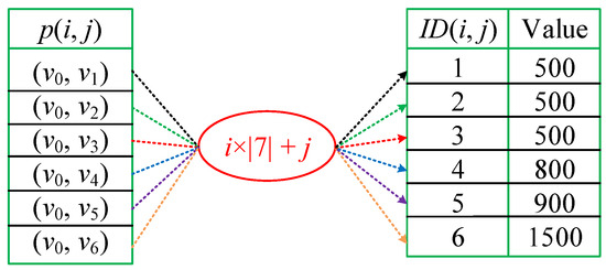
Figure 2.
Hash table construction.
3.3. The Pair-Based Lower-Bound Score Calculation
Our approach is built on a key insight. When calculating the lower-bound score of a trajectory, we can achieve more accurate results by considering both the start and end points of the trajectory, as highlighted in Lemma 1 and Lemma 2. For simplicity, refers to the pair constructed by , and refers to the distance between and .
Intuitively, when we calculate the lower-bound score of a trajectory, if we only consider one point within a trajectory, the difference between the lower-bound score and the real score may be very large, especially when the size of a trajectory is large. As a contrast, when we calculate the lower-bound score of a trajectory via considering the start/end point of a trajectory, as the start point and end point of the virtual trajectory are the same as that of , based on the spatio-temporal constraint, we can generate a more reasonable virtual trajectory. Accordingly, we can tighten up the lower-bound score . Intuitively, as the cost model we form is based on the lower-bound score of each , the pair-based lower-bound score calculation makes the model more workable.
Lemma 1.
Let be the query trajectory, and be a trajectory. When , the lower-bound score of , i.e., denoted as (), equals .
Proof.
We prove it via forming two virtual trajectories and based on and . These virtual trajectories simulate the movement of objects. Initially, and are located at and , respectively. After time units, they move towards each other and reach and , respectively, by . Along their paths, the distance between and is when , and when . Accordingly, the distance sum D() is . □
Lemma 2.
Let be the query trajectory, and be a trajectory, when , () equals .
Proof.
We prove it via forming another two virtual trajectories and based on and . Initially, and are located at and , respectively. After time units, they move towards each other and reach the same position . They stay at for time units and then move to and , with being . Under these two paths, the distance between and equals when . Accordingly, D() equals . □
It is significant to find a suitable . Take the example in Figure 3a. If is set to 1, the object arrives at using 1 time unit, and then arrives at . The distance between and equals , which is smaller than . It can arrive at before . Thus, if is set to 1, the lower-bound score is loose. If is set to 2, the object arrives at using 2 time units, and then arrives to . In addition, D() = 2.8 km, D()=, which is smaller than . It can arrive at at . If is set to 3, the object arrives at via 3 time units, and then arrives at . D() = 2.6 km, and D()=, which equals . Thus, it can arrive at at . Therefore, is set to 3. Note, in implementation, we could use a binary search to find the maximal . As it is simple, for the limitation of space, we will skip the details.
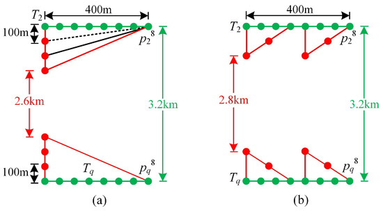
Figure 3.
Pair-based lower-bound score calculation, where (a) and (b) respectively represent the graphical depiction of the distance from to over different time units.
We also find that if the partition is applied, the corresponding lower-/upper-bound score could be further tightened. Accordingly, we propose a partition-based method to tighten the lower/upper-bound score of the trajectories. Formally, for each trajectory contained in the trajectory set , we partition into a group of sub-trajectories such that . Here, refers to the j-th sub-trajectory of , and its scale equals . also contains a set of GPS points, which are the -th generated GPS points in . refers to the number of sub-trajectories. Based on the partition result, we can update () and () to and , respectively. In addition, () and () could be calculated based on Theorem 2.
Back to the example in Figure 3a. If the partition amount is 1, () is calculated as the sum of the real location distance D(), D() and the virtual location distance . Because equals 3, D() = 3200 − 1·2·100 = 3 km, D() and D() is equal 2.8 km and 2.6 km, respectively. Then, D() = , divided into 4 parts. Each part is 125 m. So, D() is calculated as , D() = 2900 m(= + 2600) and D( + 2600). To sum up, () is 23.5 km and () is 27.7 km. (), and () are updated to 25 km and 26.2 km when the partition amount is 2.
Discussion. Pair-based partition can provide trajectories with tighter lower-bound score. However, a natural question is how to form proper partitions for different trajectories. Intuitively, if the partition amount is large, the running cost of maintaining the partition is high, but the lower-/upper-bound score is tight. In contrast, the lower-bound score is loose. It is significant to find a flexible method to self-adaptively partition trajectories based on the distance relationship among them to the query trajectory.
3.4. The Pair-Based Prediction Algorithm
In this section, we first explain the pair-based partition. Then, we explain the prediction algorithm.
The Pair-based Partition Algorithms. It is to find query result trajectories via recursively partitioning trajectories and tightening their lower-/upper-bound scores. In this way, we can find query result trajectories, as well calculate the lower-bound score of other trajectories. Intuitively, once the lower-bound scores of trajectories are computed, we can use the model (discussed later) to evaluate the running cost we spend on it, which helps us effectively assign trajectories.
In this section, we use Theorem 2 for calculating the lower-bound score of sub-trajectories. Intuitively, if more pairs are considered for lower-bound score calculation, we could obtain a tighter lower-bound score. Accordingly, we propose the concept of score. Here, we assume that each trajectory contains the set of n GPS points, with n being and being an integer. In addition, the lower-bound score of each trajectory, i.e., denoted as (), is computed based on Equation (4), with r being .
We now formally explain the partition algorithm. Firstly, we access each , and compute and as the manner discussed in Theorem 2. After calculating the lower-bound scores/upper-bounds of all trajectories, we search , i.e., the trajectory with the -th lowest upper-bound score, use () for pruning trajectories in . In other words, for each trajectory , its lower-bound score is larger than (). It is not a query result trajectory, and we remove it to the set .
For the reminders, we split each element in into two sub-trajectories with an equal scale, and update their lower-bound score based on Equation (4). Again, for each of them, if existing k trajectories have an upper-bound score lower than it, it is removed from to the set . From then on, we repeat the above operations until the number of trajectories in reduces to k. At that moment, we can use these k trajectories as query result trajectories in the current window. Note, during the partition, we can form the corresponding PDSP structure for each trajectory.
The PDSP-based Prediction. After we form the PDSP for each trajectory, we are going to predict the earliest moment, i.e., denoted as , each trajectory may become a query result trajectory. In this way, we need not to monitor before . Specially, we scan each trajectory and calculate based on Theorem 1. After calculation, we use a prior queue to maintain these trajectories based on of each . As the algorithm is simple, we skip the details to save space.
Theorem 1.
Trajectories , and , D() are no smaller than D() after δ time units with δ being computed based on the in-Equation () ≤ D().
Proof.
We assume that is partitioned into sub-trajectories . Theorem 1 is proved under the following two cases: (i) ; (ii) . Under case (i), we use the manner discussed in Theorem 1 to find the maximal . Under cases (ii), () equals ()+ ()+ (), while () equals D()+(). We could find the maximal via the Equation (). □
We want to highlight that, once of each is calculated, we can ensure that cannot become a query result trajectory before . In addition, we can evaluate the running cost we will spend on it. It is convenient to evaluate its importance to the query result sets and make a reasonable partition based on the prediction result.
3.5. Trajectory Set Partition Algorithm
As the number of trajectories is usually large, it is difficult to process a large number of trajectories over a single server. Thus, in this section, we study how to form a reason partition that partitions trajectories into a group of servers, making sure that the workload of each server is as similar as possible. In order to achieve this goal, we first form a model to evaluate the running cost of each trajectory.
Specially, let be a trajectory in the trajectory set , be the number of points we access when evaluating its prediction moment, and be the prediction moment of . After n time units are passed, the excepted time we access is . Accordingly, the excepted running cost of maintaining could be calculated via Equation (5). In addition, the excepted running cost of maintaining all trajectories could be computed based on Equation (6).
After explaining the cost model, we now formally explain the partition algorithm. Our goal is to make the workload of each server is as the same as possible.
Let be the set of servers. For each server , we use to record the current workload of , and servers in are sorted in ascended order by their workload. We use the greedy algorithm to form the partition. Specially, we scan each trajectory , compute its excepted running cost via Equation (6), allocate it to the server with minimal workload, and finally update .
3.6. The Incremental Maintenance Algorithms
In this section, we first discuss the incremental algorithm over each server, i.e., the local incremental maintenance algorithm. Its function is to update the prediction moment of trajectories in each server. Next, we explain the global incremental maintenance algorithm. Its function is to guarantee the workload of each server is as similar as possible.
3.6.1. The Local Incremental Maintenance Algorithm
In the following, we propose the algorithm INC-PDSP, which explains how PDSP is applied for supporting the data stream. Here, and are two inverted lists that maintain non-query result trajectories and query result trajectories, respectively. Our algorithm is proposed based on the following observation. That is, the prediction moment of a trajectory is computed based on the assumption that trajectories in move far away from . It is actually not true in real applications. A moment of thought could reveal that if is not rapidly increased, we can delay the prediction moment updating of trajectories. Here, refers to the k-th lowest score among all trajectories in the query result set.
We now formally provide the algorithm details. We associate with a variable named with being the inverted list that maintains all non-query result trajectories. It records the sum of time units we can delay. Its value is set to 0 at the moment is constructed. Whenever one time unit is passed, we update to , where is computed based on Equation (7). Here, refers to the k-th highest score among elements in at the last time unit. D() refers to the predicted score of at the current time unit. D()− refers to the difference between the predicted and real . In addition, we associate each element with a variable named . Its value equals at the moment ’s prediction moment is updated. Whenever one time unit is passed, we update based on Equation (7). Next, we check whether the element located at the top of satisfying . If the answer is yes, we update its prediction moment. Lastly, we set to .
3.6.2. The Global Incremental Maintenance Algorithm
We should monitor the workload of each server so as to guarantee the balance of the system. Thus, we should update of each server whenever one trajectory T in is passed. Specially, let T be the trajectory we should evaluate. We first update its prediction moment. Next, we re-calculate its excepted running cost and update based on the re-calculating result.
The reason we monitor the workload of each server is we should re-allocate trajectories if the workload difference among different servers is so large. In our paper, if , we should re-allocate trajectories in the server and . Here, and refer to the server with maximal and minimal workload in . When re-allocating, we scan trajectories in and remove each scanned trajectory from to . When is reduced to less than , the algorithm is terminated.
4. Performance Evaluation
In this section, we conduct extensive experiments to demonstrate the efficiency of the RNDLP framework. The experiments are based on both real datasets and synthetic datasets. In the following, we first explain the datasets used in our experiments and the settings of our experiments and then report our findings.
4.1. Experiment Settings
Datasets. In total, four datasets are utilized in our experiments, comprising three real datasets: Beijing, Porto, and NYC, and a synthetic dataset named Normal. Beijing is sourced from the Microsoft T-Drive project, encompassing GPS trajectories of 10,357 taxis recorded from 2 February to 8 February 2008. Porto consists of 1,710,671 trajectories, describing the trajectory of 442 taxis from 7 January 2013 to 30 June 2014 in the city of Porto. NYC is obtained from the New York City Taxi and Limousine Commission, containing 2.36 GB of trip records. Accordingly, we generate a group of trajectories based on these records. Each record corresponds to a trajectory, where the start point and end point of the trajectory is set based on the pick-up point and drop-off point of the record. The trajectory is generated based on the shortest path based on the pick-up point and drop-off point of the record.
Normal is a synthetic trajectory dataset created by simulating the trajectories of moving objects on urban roads. The road network under these four datasets are shown in Table 1. We pre-process these datasets by retaining only four attributes, namely taxi ID, location longitude, location latitude, and timestamp. Note, the running time of our proposed framework is unrelated with the scale of the graph. The reason behind it is we use a hash table to maintain the shortest path among every two vertexes, and we can use running cost to caluate the distance between two point over road network.

Table 1.
Road network information.
Experimental Methodology. In our study, we first load the road network, the hash table, as well as all trajectories into the memory. Next, we scan each trajectory in the trajectory set, compute its score or lower-bound score. After scanning, we assign these trajectories to different servers based on the model discussed before. From then on, we monitor the alarm time of each trajectory and update the scores of trajectories with their alarm time being the current time unit. When all trajectory are processed, we report the total running time.
Parameters. In our study, we evaluate the performance of different algorithms under four parameters: N, n, k, and . Here, N denotes the number of trajectories within the trajectory set ; n represents the number of GPS points within each trajectory; k is the input parameter for CKTRN; and denotes the maximal traveling speed of objects per time unit. The parameter settings are presented in Table 2, with the default values bolded.
Table 2.
Parameter settings.
Performance Metrics. The updating time is employed as the main performance metric. It refers to the average time used to process newly generated GPS points.
Competitors. In addition to the algorithm included in the RNDLP framework, we also implement a baseline algorithm named BASE. Note, the BASE algorithm updates scores of all trajectories whenever one time unit is passed. All the algorithms are implemented with C++, and all the experiments are conducted on 6226R CPU with 256 GB memory, running Microsoft Windows 10.
4.2. Performance Comparison
Updating Cost Comparison. In this section, we compare the performance of RNDLP with its competitors when supporting CKTRN under a data stream.
We present the running time of all algorithms under different k values in Figure 4a–d. Across all evaluated k values, RNDLP consistently outperforms BASE for all four datasets. For instance, in the PORTO dataset, the running time of RNDLP is only of BASE, in the BEIJING dataset, it is of BASE, and in the NORMAL dataset, it is of BASE. The notable improvement arises from RNDLP considering spatio-temporal correlation among GPS points in each trajectory. The corresponding virtual trajectory is closer to the real trajectory, allowing it to provide trajectories with tight score bounds by accessing a small number of GPS points. In addition, RNDLP uses hash table to maintain the distance among every two vertexes over road network.
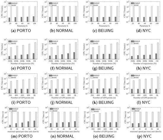
Figure 4.
Running time comparison of different algorithms under different datasets.
Furthermore, we report the running time of different algorithms under various N values in Figure 4e–h. As N increases, the running time of BASE sharply rises because BASE has to access all trajectories whenever the window slides. In contrast, RNDLP is not sensitive to N values thanks to the predictive nature of its employed algorithms. It does not need to maintain N trajectories in real time, resulting in a much more stable performance under various parameter settings. Besides the reasons discussed above, another important reason is we use a cost model to partition trajectories into different servers. In this way, the overhead of each server is roughly the same. As a contrast, BASE does not consider how to equally partition trajectories. Thus, in many cases, trajectories are skewed when distributed in each server. Thus, the total running cost of BASE is higher than that of RNDLP.
The running time of different algorithms under various n values is reported in Figure 4i–l. Here again, RNDLP outperforms its counterparts. Notably, BASE’s running time gradually increases with the growth of n since it has to access more GPS points when trajectories’ prediction moments are updated. Conversely, RNDLP’s running time does not change significantly with increased n values. This is because the larger the n, the larger the distance among starting points of objects’ trajectories to their end points. In this way, RNDLP could accurately calculate score bounds of trajectories via setting to a small value. In addition, as RNDLP could dynamically adjust prediction moment of trajectories, it could further reduce the cost of incremental maintenance.
The running time of different algorithms under different is reported in Figure 4m–p. We find that RNDLP performed better again. In addition, BASE is not sensitive to . The reason is BASE does not consider speed constraint. The running time of RNDLP gradually increases, but still spends much lower cost than the BASE algorithm. This is because the larger the , the looser the lower-bound score BASE could provide. However, as is usually not high in most applications, RNDLP is the most efficient in most cases (Table 3).
Table 3.
Performance analysis of different similarity measures.
To sum up, RNDLP is both stable and efficient. It requires the lowest running time to support continuous k-similarity search over road network compared with the BASE algorithm.
5. Conclusions
In this paper, we propose a novel framework named SLBP to support continuous k-similarity trajectories search over road network. The framework can efficiently return query result trajectories by accessing only a few GPS points from a subset of trajectories within the entire trajectory set. Additionally, we propose a pair-based method to enhance algorithm performance. Through the calculation of lower-bound scores for trajectories, we observe that processing a small number of trajectories with each slide of the window is sufficient. As a result, our framework efficiently supports continuous k-similarity trajectories search over data streams. We conducted extensive experiments to evaluate the performance of our proposed algorithms on several datasets. The results consistently demonstrate the superior performance of our proposed algorithms.
Author Contributions
This research was jointly performed by H.J., S.T., R.Z. and B.W. Methodology, H.J.; resources, H.J.; writing—original draft, S.T.; supervision, R.Z. and B.W. All authors have read and agreed to the published version of the manuscript.
Funding
This research was funded by the Social Science Planning Fund of Liaoning Province (No. L21BGL042).
Data Availability Statement
Publicly available datasets were analyzed in this study. The data can be found here: BEIJING: https://www.microsoft.com/en-us/research/publication/t-drive-trajectory-data-sample/ (accessed on 7 January 2024); PORTO: https://tianchi.aliyun.com/dataset/94216 (accessed on 7 January 2024); NYC: https://opendata.cityofnewyork.us/ (accessed 7 January 2024).
Conflicts of Interest
The authors declare no conflict of interest.
Abbreviations
The following abbreviations are used in this manuscript:
| the trajectory | |
| the query trajectory | |
| D() | the score of |
| () | the lower-bound score of |
| () | the upper-bound score of |
| the j-th generated GPS point in | |
| a sub-trajectory of with first/last generated point / | |
| () | the lower-bound score of under -score |
| the predicted moment of |
References
- Chen, Y.; Zhang, H.; Sun, W.; Zheng, B. RNTrajRec: Road Network Enhanced Trajectory Recovery with Spatial-Temporal Transformer. In Proceedings of the 39th IEEE International Conference on Data Engineering, ICDE 2023, Anaheim, CA, USA, 3–7 April 2023; pp. 829–842. [Google Scholar] [CrossRef]
- Du, Y.; Hu, Y.; Zhang, Z.; Fang, Z.; Chen, L.; Zheng, B.; Gao, Y. LDPTrace: Locally Differentially Private Trajectory Synthesis. Proc. VLDB Endow. 2023, 16, 1897–1909. [Google Scholar] [CrossRef]
- Hwang, J.R.; Kang, H.Y.; Li, K.J. Spatio-temporal similarity analysis between trajectories on road networks. In Proceedings of the Perspectives in Conceptual Modeling: ER 2005 Workshops AOIS, BP-UML, CoMoGIS, eCOMO, and QoIS, Klagenfurt, Austria, 24–28 October 2005; Proceedings 24. Springer: Cham, Switzerland, 2005; pp. 280–289. [Google Scholar]
- Tiakas, E.; Papadopoulos, A.; Nanopoulos, A.; Manolopoulos, Y.; Stojanovic, D.; Djordjevic-Kajan, S. Searching for similar trajectories in spatial networks. J. Syst. Softw. 2009, 82, 772–788. [Google Scholar] [CrossRef]
- Kim, S.W.; Won, J.I.; Kim, J.D.; Shin, M.; Lee, J.; Kim, H. Path prediction of moving objects on road networks through analyzing past trajectories. In Proceedings of the Knowledge-Based Intelligent Information and Engineering Systems: 11th International Conference, KES 2007, XVII Italian Workshop on Neural Networks, Vietri sul Mare, Italy, 12–14 September 2007; Proceedings, Part I 11. Springer: Cham, Switzerland, 2007; pp. 379–389. [Google Scholar]
- Jiang, J.; Xu, C.; Xu, J.; Xu, M. Route planning for locations based on trajectory segments. In Proceedings of the 2nd ACM SIGSPATIAL, San Francisco, CA, USA, 31 October 2016; pp. 1–8. [Google Scholar]
- Li, T.; Chen, L.; Jensen, C.S.; Pedersen, T.B. TRACE: Real-time Compression of Streaming Trajectories in Road Networks. Proc. VLDB Endow. 2021, 14, 1175–1187. [Google Scholar] [CrossRef]
- Li, T.; Chen, L.; Jensen, C.S.; Pedersen, T.B.; Gao, Y.; Hu, J. Evolutionary Clustering of Moving Objects. In Proceedings of the 2022 IEEE 38th ICDE, Kuala Lumpur, Malaysia, 9–12 May 2022; pp. 2399–2411. [Google Scholar]
- Li, T.; Huang, R.; Chen, L.; Jensen, C.S.; Pedersen, T.B. Compression of Uncertain Trajectories in Road Networks. Proc. VLDB Endow. 2020, 13, 1050–1063. [Google Scholar] [CrossRef]
- Wu, J.; Li, T.; Chen, L.; Gao, Y.; Wei, Z. SEA: A Scalable Entity Alignment System. In Proceedings of the 46th International ACM SIGIR Conference on Research and Development in Information Retrieval, SIGIR 2023, Taipei, Taiwan, 23–27 July 2023; Chen, H., Duh, W.E., Huang, H., Kato, M.P., Mothe, J., Poblete, B., Eds.; ACM: New York, NY, USA, 2023; pp. 3175–3179. [Google Scholar] [CrossRef]
- Tang, L.A.; Zheng, Y.; Yuan, J.; Han, J.; Leung, A.; Hung, C.C.; Peng, W.C. On discovery of traveling companions from streaming trajectories. In Proceedings of the 2012 IEEE 28th ICDE, Arlington, VA, USA, 1–5 April 2012; pp. 186–197. [Google Scholar]
- Yang, X.; Wang, B.; Yang, K.; Liu, C.; Zheng, B. A Novel Representation and Compression for Queries on Trajectories in Road Networks. IEEE Trans. Knowl. Data Eng. 2018, 30, 613–629. [Google Scholar] [CrossRef]
- Sacharidis, D.; Skoutas, D.; Skoumas, G. Continuous monitoring of nearest trajectories. In Proceedings of the 22nd ACM SIGSPATIAL, Dallas, TX, USA, 4–7 November 2014; pp. 361–370. [Google Scholar]
- Yu, X.; Zhu, S.; Ren, Y. Continuous trajectory similarity search with result diversification. Future Gener. Comput. Syst. 2023, 143, 392–400. [Google Scholar] [CrossRef]
- Pan, Z.; Chao, P.; Fang, J.; Chen, W.; Xu, J.; Zhao, L. Garden: At real-time processing framework for continuous top-k trajectory similarity search. Knowl. Inf. Syst. 2023, 65, 3777–3805. [Google Scholar] [CrossRef]
- Zhang, D.; Chang, Z.; Wu, S.; Yuan, Y.; Tan, K.; Chen, G. Continuous Trajectory Similarity Search for Online Outlier Detection. IEEE Trans. Knowl. Data Eng. 2022, 34, 4690–4704. [Google Scholar] [CrossRef]
- Jin, P.; Cui, T.; Wang, Q.; Jensen, C.S. Effective similarity search on indoor moving-object trajectories. In Proceedings of the Database Systems for Advanced Applications: 21st International Conference, DASFAA 2016, Dallas, TX, USA, 16–19 April 2016; Proceedings, Part II 21. Springer: Cham, Switzerland, 2016; pp. 181–197. [Google Scholar]
- Tang, J.; Deng, M.; Huang, J.; Liu, H.; Chen, X. An automatic method for detection and update of additive changes in road network with GPS trajectory data. ISPRS Int. J. Geo-Inf. 2019, 8, 411. [Google Scholar] [CrossRef]
- Zhu, R.; Xiao, M.; Wang, B.; Yang, X.; Xia, X.; Zong, C.; Qiu, T. Continuous k-Similarity Trajectories Search over Data Stream. In Lecture Notes in Computer Science, Proceedings of the Database Systems for Advanced Applications—28th International Conference, DASFAA 2023, Tianjin, China, 17–20 April 2023; Proceedings, Part I; Wang, X., Sapino, M.L., Han, W., Abbadi, A.E., Dobbie, G., Feng, Z., Shao, Y., Yin, H., Eds.; Springer: Cham, Switzerland, 2023; Volume 13943, pp. 273–282. [Google Scholar] [CrossRef]
- Güting, R.H.; Behr, T.; Xu, J. Efficient k-nearest neighbor search on moving object trajectories. VLDB J. 2010, 19, 687–714. [Google Scholar] [CrossRef]
- Li, Y.S.; Li, T.Y.; Zhou, J.G.; Huang, B.N. Double-consensus based distributed optimal energy management for multiple energy hubs. Appl. Sci. 2018, 8, 1412. [Google Scholar] [CrossRef]
- Chen, L.; Özsu, M.T.; Oria, V. Robust and fast similarity search for moving object trajectories. In Proceedings of the 2005 ACM SIGMOD, Baltimore, MD, USA, 14–16 June 2005; pp. 491–502. [Google Scholar]
- Gawde, G.; Pawar, J. Similarity search of time series trajectories based on shape. In Proceedings of the ACM India Joint International Conference on Data Science and Management of Data, Goa, India, 11–13 January 2018; pp. 340–343. [Google Scholar]
- Zhu, R.; Wang, B.; Yang, X.; Zheng, B.; Wang, G. SAP: Improving Continuous Top-K Queries Over Streaming Data. IEEE Trans. Knowl. Data Eng. 2017, 29, 1310–1328. [Google Scholar] [CrossRef]
Disclaimer/Publisher’s Note: The statements, opinions and data contained in all publications are solely those of the individual author(s) and contributor(s) and not of MDPI and/or the editor(s). MDPI and/or the editor(s) disclaim responsibility for any injury to people or property resulting from any ideas, methods, instructions or products referred to in the content. |
© 2024 by the authors. Licensee MDPI, Basel, Switzerland. This article is an open access article distributed under the terms and conditions of the Creative Commons Attribution (CC BY) license (https://creativecommons.org/licenses/by/4.0/).