A New Family of Distributions Based on Proportional Hazards

Abstract

In this article, we introduce a new family of symmetric-asymmetric distributions based on skew distributions and on the family of order statistics with proportional hazards. This new family of distributions is able to fit both unimodal and bimodal asymmetric data. Furthermore, it contains, as special cases, the symmetric distribution and the “skew-symmetric” family, and therefore the skew-normal distribution. Another interesting feature of the family is that the parameter controlling the distributional shape in bimodal cases takes values in the interval (0, 1); this is an advantage for computing maximum likelihood estimates of model parameters, which is performed by numerical methods. The practical utility of the proposed distribution is illustrated in two real data applications.

1. Introduction

A seminal paper by [1] revealed the main properties of the “skew-normal” distribution whose probability density function (pdf) is given by

$${\varphi }_{SN}(z;\lambda )=2\varphi \left(z\right)\mathsf{\Phi }\left(\lambda z\right),z\in \mathbb{R},$$

where $\mathsf{\Phi }$ and $\varphi$ denote the cumulative and density functions of the standard normal distribution, respectively. Here, $\lambda$ is a parameter that controls the asymmetry of the random variable Z. Generally this is denoted by SN$\left(\lambda \right)$. Since this work was published, numerous publications have been based on this model, primarily [2,3,4,5,6,7,8,9].

An important lemma demonstrated by [1] represents a fundamental result in the development of asymmetric and symmetric models for both unimodal and bimodal cases. This lemma is presented below.

Lemma 1.

Let$f_0$be a pdf symmetrical around zero and a distribution function G such that$G^{\prime }$exists and is a symmetric (around zero) density function; then

$$\begin{array}{c}\hfill f_Z(z;\lambda )=2f_0\left(z\right)G\left(\lambda z\right),z\in \mathbb{R}\end{array}$$

is a density function for any$\lambda \in \mathbb{R}$. This will be denoted by$S{f}_0\left(\lambda \right)$.

1.1. Asymmetric Models of Fractional Order Statistics

The study of asymmetric models based on order statistics goes back to [10], who introduced a model called the “Lehmann alternative”, which originated from the distribution of the maximum in the sample. It later became an alternative for distributions presenting a high degree of asymmetry and/or kurtosis. This family of distributions is represented by the distribution function

$${\mathcal{F}}_F(z;\alpha )={\left\{F\left(z\right)\right\}}^{\alpha },z\in \mathbb{R},$$

where F is a cumulative distribution function (cdf) and $\alpha$ is a rational number. For $\alpha \in \mathbb{N}$, we have the distribution function of the maximum in the sample.

Subsequently, [11] introduced the distribution of fractional order statistics, which is defined by the pdf

$${\psi }_F(z;\alpha )=\alpha f\left(z\right){\left\{F\left(z\right)\right\}}^{\alpha -1},z\in \mathbb{R},$$

where $\alpha \in {\mathbb{R}}^{+}$ is a shape parameter and F is an absolutely continuous distribution function with pdf $f=dF$. This is called the power-symmetric (PS) model. Derivations and properties of the distributions of order statistics have been widely discussed by [12,13,14], among others. One important special case follows when $f=\varphi$: this is called the power-normal (PN) distribution (see [14]). Ref. [15] derived the expected (Fisher) information matrix for the PN distribution and showed that it is nonsingular at the vicinity of symmetry ($\alpha =1.0$), in contrast to the case of SN density, for which the Fisher formation matrix is singular at $\lambda =1.0$.

1.2. Asymmetric Bimodal Models

Several fields of science provide data that cannot be modeled or fitted with distributions such as skew-normal or fractional order statistics because the nature of these data leads to bimodal behaviors; these distributions have good performance only for unimodal cases. In many areas, such as health sciences, engineering, economics, among others, it is common to find data sets that present bimodal behaviors; thus, it is required other model alternatives that besides being able to capture a possible bimodality, do not present identifiability problems of the parameters, which are often proposals that come from mixtures of distributions. Consequently, this research is motivated with the interest of estimating, in a simple way, the parameters of the model that we propose and that has the faculty of fitting symmetric or asymmetric bimodal data, being thus a proposal that opens the possibility of new researches in these areas.

Models of this type have been studied by [16], who introduced the bimodal extension of the skew-normal model, called the “two-pieces skew-normal (TN) model”. This model is denoted by TN$\left(\lambda \right)$, whose pdf is represented by

$$g(z;\lambda )=c_{\lambda }\varphi \left(z\right)\mathsf{\Phi }\left(\lambda \right|z\left|\right),$$

(1)

where $\lambda$ is a real number and $c_{\lambda }=2\pi /(\pi +2arctan\left(\lambda \right))$ is a normalizing constant. For $\lambda >0$, Kim demonstrates that model (1) is bimodal and symmetric around zero.

Ref. [17] developed the asymmetric bimodal model termed “the extended two-pieces skew-normal (ETN) model”, with a pdf given by

$$h(z;\theta )=2c_{\lambda }\varphi \left(z\right)\mathsf{\Phi }\left(\lambda \left|z\right|\right)\mathsf{\Phi }\left(\beta z\right),$$

(2)

where $\beta$ and $\lambda$ are real numbers and $c_{\lambda }$ is a normalizing constant. The model is denoted by ETN$(\lambda ,\beta )$ and is an asymmetric extension of Kim’s model.

The proportional hazards model was introduced by [18] and is very important in survival analysis. Although [18] used this model to introduce covariables, it can also be used to introduce a shape parameter into the base distribution (see [19]). One example is the Burr XII distribution (see [20]), which can be obtained as a proportional hazards model from the base distribution function. The main object of this paper is to use this proportional hazards methodology to propose a new family of uni-/bimodal distributions, based on the power- symmetric family of distributions.

The paper is organized as follows. In Section 2, the extended skew model distribution with proportional hazards is derived, and its density function, special cases and moments are presented. In Section 3, parameter estimation is considered using maximum likelihood (ML). Observed and Fisher information matrices are derived, and it is shown that the Fisher information matrix is nonsingular. In Section 4, we perform a small-scale simulation study. In Section 5, two real data sets are analyzed using the proposed distribution and some other competing distributions to illustrate their applicability.

2. Extended Skew Model with Proportional Hazard

Following similar guidelines as in [10,11], we define the density function of the order statistics with proportional hazard.

Let F be a continuous cdf with pdf f, continuous and symmetric around zero, and hazard function $h=f/(1-F)$. We say that Z has a distribution with proportional hazards, associated with the cdf F and pdf f, and parameter $\alpha >0$ if its pdf is given by the expression

$${\phi }_F(z;\alpha )=\alpha f\left(z\right){\{1-F\left(z\right)\}}^{\alpha -1},z\in \mathbb{R},$$

(3)

where $\alpha$ is a positive real number and F is a continuous distribution function with density function $f=dF,$ continuous and symmetrical around zero. The PS distribution with proportional hazards is denoted by PSH$\left(\alpha \right)$. For $f=F^{\prime }$, a pdf continuous and symmetric around zero, the density (3) matches the density of the variable $Z=-Y$ where $Y\sim \mathrm{PS}\left(\alpha \right)$.

The cdf of the PSH model is given by

$$\mathbb{F}\left(z\right)=1-{\{1-F\left(z\right)\}}^{\alpha },z\in \mathbb{R}.$$

The expression proportional hazards model must be understood in the sense that the hazard function of this model concerning the function $\mathbb{F}\left(z\right)$ is

$$h(X,F,\alpha )=\alpha h\left(x\right).$$

When $F=\mathsf{\Phi }$, we get the PN distribution with proportional hazards, which is denoted by PNH$\left(\alpha \right)$. This model also represents an alternative for modeling data with skewness and kurtosis outside the permitted ranges for normal function.

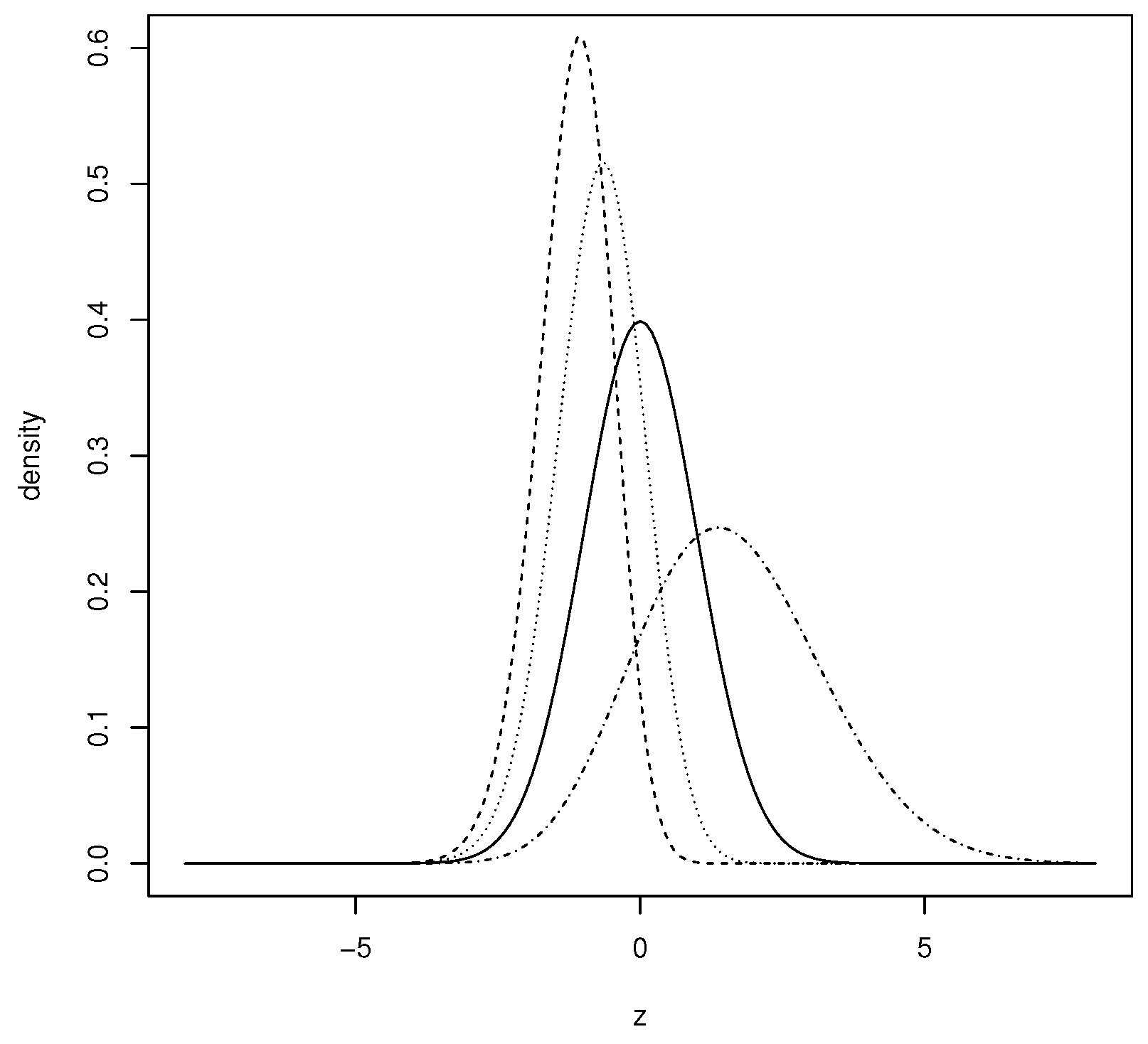
Figure 1 depicts how parameter $\alpha$ controls the skewness and kurtosis of the PNH$\left(\alpha \right)$ model.

Figure 1. Plots of the PNH$\left(\alpha \right)$ distribution with $\alpha =$ 0.25 (dotted and dashed line), 1 (solid line), 2 (dashed line) and 3 (dotted line).

The PNH model is suitable for fitting asymmetric unimodal data. Although this model is more flexible than the normal model, it is unsuitable for fitting a bimodal data set. A more flexible model than the PNH is as defined below, which has the ability to fit unimodal and well as bimodal data. This model is obtained from the PNH$\left(\alpha \right)$ model.

We define the extended proportional hazard model by the pdf

$$\phi (z;\alpha )=\alpha f\left(z\right){\left\{2(1-F(\left|z\right|\left)\right)\right\}}^{\alpha -1},z\in \mathbb{R},$$

(4)

where $\alpha \in {\mathbb{R}}^{+}$, F is an absolutely continuous cdf with pdf $f=F^{\prime }$, which is symmetrical around zero. We use the notation EPSH$\left(\alpha \right)$.

Result 1.

If $Z\sim \mathrm{EPSH}\left(\alpha \right)$, then the model (4) is symmetrical.

Result 2.

If $Z\sim \mathrm{EPSH}\left(\alpha \right),$ then the cdf of Z is given by:

$${\mathcal{F}}_F(z;\alpha )=\left\{\begin{array}{cc}\frac{1}{2}{\left\{2F\left(z\right)\right\}}^{\alpha },\hfill & \mathrm{if}z<0,\hfill \\ \frac{1}{2}{\left\{2(1-F(z\left)\right)\right\}}^{\alpha },\hfill & \mathrm{if}z\ge 0.\hfill \end{array}\right.$$

Result 3.

Let $Z\sim \mathrm{EPSH}\left(\alpha \right)$ and $U\sim u(0,1)$. Then, using the inversion method, we can obtain a random variable with distribution $Z\sim \mathrm{EPSH}\left(\alpha \right)$. This variable can be obtained by the expression

$$Z=\left\{\begin{array}{cc}{F}^{-1}\left[\frac{1}{2}{\left(2U\right)}^{1/\alpha }\right],\hfill & \mathrm{with}U<1/2\mathrm{and}Z<0,\hfill \\ F^{-1}\left[1-\frac{1}{2}{\left(2U\right)}^{1/\alpha }\right],\hfill & \mathrm{with}U\ge 1/2\mathrm{and}Z\ge 0,\hfill \end{array}\right.$$

(5)

where $F^{-1}$ is the inverse function of F.

2.1. Skew-EPsH (SEPSH) Model

Although the EPSH model is adequate for fitting bimodal data sets, it is not suitable when the data set presents asymmetric bimodality. However, supported by the results given in [1], we can obtain a more general model that achieves asymmetric bimodality.

Based on models (4) and (2), we now introduce a new family of distributions with the special feature that for certain distributions (e.g., normal), it can fit asymmetrical uni and bimodal data sets. This new family of distributions has pdf

$${\phi }_{F-G}(z;\alpha ,\beta )=2\alpha f\left(z\right){\left\{2(1-F(\left|z\right|\left)\right)\right\}}^{\alpha -1}G\left(\beta z\right),z\in \mathbb{R},$$

(6)

where $\alpha \in {\mathbb{R}}^{+},$$\beta \in \mathbb{R},$F is a continuous distribution function with density $f=F^{\prime },$ which is symmetric around zero, and G is a continuous and symmetric cdf with pdf $G^{\prime }$, symmetric around zero. This new family of distributions is called the asymmetric extended family with proportional hazards. Note that when $\alpha =1,$ we have the “skew-symmetric” distribution, i.e., this new model can be seen as a generalization of the “skew-symmetric” model and the models of order statistics for the case of proportional hazards.

The proof that function (6) is a density follows from Lemma 1 by taking $f_0\left(z\right)=\alpha f\left(z\right){\left\{2(1-F(\left|z\right|\left)\right)\right\}}^{\alpha -1},$ which is symmetric around zero. Therefore, this new family of distributions belongs to the “skew-symmetric” family, and as $f_0$ belongs to the exponentiated family (see [13]) or family of order statistics [11], this model will be called “skew-power-symmetric (SPS)” and we will be denoted by SPS$(\alpha ,\beta )$.

Result 4.

$\mathrm{SPS}(1,\beta )=S{f}_0\left(\beta \right)$.

The proof of this result is immediate since $f=dF=f_0$ is symmetric around zero. Therefore, the “skew-symmetric” distribution of Azzalini is a special case of the SPS$(\alpha ,\beta )$ distribution.

2.2. Skew-Power-Normal Model

Taking $F=G=\varphi$ in (6) leads to the model

$${\phi }_{\mathsf{\Phi }}(z;\alpha ,\beta )=2\alpha \varphi \left(z\right){\left\{2(1-\mathsf{\Phi }(\left|z\right|\left)\right)\right\}}^{\alpha -1}\mathsf{\Phi }\left(\beta z\right),z\in \mathbb{R},$$

(7)

which will be called “skew-power-normal (SPN)” model, and will be denoted by SPN$(\alpha ,\beta )$.

• Properties

The following properties are obtained directly from the model (7).

Property 1.

SPN(1, 0) = N(0, 1).

Property 2.

SPN(1, β) = SN(β).

Property 3.

SPN(α, 0) = PNH(α).

Property 4.

SPN(2, β) = a × SN(β) − b × ETN(β) with a and b positive constants.

Property 5.

SPN(2, 0) = a × N(0, 1) − b × TN(1) with a and b positive constants.

Result 5.

If $Z\sim \mathrm{SPN}(\alpha ,\beta )$, then for $\beta \ne 0$, its density function is unimodal asymmetric for $\alpha \ge 1$ and asymmetric bimodal for $\alpha <1$.

Proof of Result 5. 

Differentiating $f_0\left(z\right)=\alpha \varphi \left(z\right){\left\{2(1-\mathsf{\Phi }(\left|z\right|\left)\right)\right\}}^{\alpha -1}$ with respect to z and equating to zero, we obtain that the points where the maxima and minima occur are the solutions of the equations

$$\left\{\begin{array}{cc}(\alpha -2)log[1-\varphi (\left|x\right|\left)\right]+log\left(\varphi \right(\left|x\right|\left)\right)=0,\hfill & \mathrm{if}\alpha \ge 1,\hfill \\ (1-\alpha )\varphi \left(\right|x\left|\right)=\left|x\right|(1-\mathsf{\Phi }(\left|x\right|\left)\right),\hfill & \mathrm{if}\alpha <1.\hfill \end{array}\right.$$

Then, $f_0$ is unimodal for $\alpha \ge 1$ and bimodal for $\alpha <1$. In addition, as $f_0$ is symmetric, then this density will be bimodal symmetric for $\alpha <1$. Therefore, we conclude that ${\phi }_{\mathsf{\Phi }}(z;\alpha ,\beta )$ is asymmetric bimodal if $\alpha <1$ and asymmetric unimodal otherwise. □

This feature makes the model attractive for fitting data presenting bimodality, since the parameter range is very short (between 0 and 1), making it advantageous for computational procedures taking into account that the starting point of the process maximizing the log-likelihood function is determined more accurately.

The Location-Scale Case

Consider a random variable $Z\sim \mathrm{SPN}(\alpha ,\beta )$, with $\alpha \in {\mathbb{R}}^{+}$ and $\beta \in \mathbb{R}$. The family of distributions with location-scale parameters for the SPN distribution is defined as the distribution of $X=\xi +\eta Z$ for $\xi \in \mathbb{R}$ and $\eta >0$, and its density function is given by

$${\phi }_{\mathsf{\Phi }}(x;\xi ,\eta ,\alpha ,\beta )=\frac{2\alpha }{\eta }\varphi \left(\frac{x-\xi }{\eta }\right){\left\{2\left(1-\mathsf{\Phi }\left(\left|\frac{x-\xi }{\eta }\right|\right)\right)\right\}}^{\alpha -1}\mathsf{\Phi }\left\{\beta \left(\frac{x-\xi }{\eta }\right)\right\},x\in \mathbb{R},$$

(8)

where $\xi$ is the location parameter and $\eta$ is the scale parameter. We use the notation $\mathrm{SPN}(\xi ,\eta ,\alpha ,\beta )$.

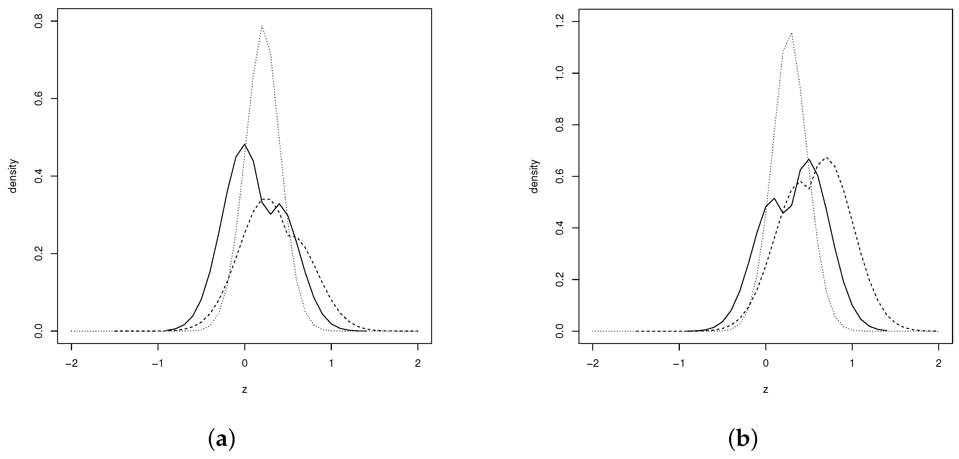
Figure 2 illustrates the behavior of the pdf (8) for different values of $\xi ,$$\eta ,$$\alpha$ and $\beta$. As can be seen from the figure, the shape of the bimodality depends on the parameters $\alpha$ and $\beta$.

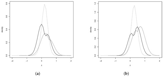
Figure 2. Plots of the distributions: (a) SPN$(0.25,0.15,0.25,-1)$ (solid line), SPN$(0.5,0.25,0.5,-1)$ (dashed line) and SPN$(0.25,0.25,1.25,-1)$ (dotted line) (b) SPN$(0.25,0.15,0.25,1)$ (solid line), SPN$(0.5,0.25,0.5,1)$ (dashed line) and SPN$(0.25,0.25,1.25,1)$ (dotted line).

2.3. Moments

The following expressions allow the calculation of the moments of a random variable with SPN$(\alpha ,\beta )$ distribution

$$\mathbb{E}\left(Z^r\right)=\left\{\begin{array}{cc}{2}^{\alpha }{\mu }_r\left(\alpha \right),\hfill & \mathrm{if}r\mathrm{is}\mathrm{even},\hfill \\ 2^{\alpha }\left[2{\mu }_r(\alpha ,\beta )-{\mu }_r\left(\alpha \right)\right],\hfill & \mathrm{if}r\mathrm{is}\mathrm{odd},\hfill \end{array}\right.$$

where

$${\mu }_r\left(\alpha \right)=\alpha {\int }_{-\infty }^0{z}^r\varphi \left(z\right){\left\{\mathsf{\Phi }\left(z\right)\right\}}^{\alpha -1}dz\mathrm{and}{\mu }_r(\alpha ,\beta )=\alpha {\int }_{-\infty }^0{z}^r\varphi \left(z\right){\left\{\mathsf{\Phi }\left(z\right)\right\}}^{\alpha -1}\mathsf{\Phi }\left(\beta z\right)dz.$$

The central moments $\acute{{\mu }_r}=E{(Z-E\left(Z\right))}^r$ for $r=2,3,4$ can be calculated from the expressions:

$$\acute{{\mu }_2}={\mu }_2-{\mu }_1^2,\acute{{\mu }_3}={\mu }_3-3{\mu }_2{\mu }_1+2{\mu }_1^3\mathrm{and}\acute{{\mu }_4}={\mu }_4-4{\mu }_3{\mu }_1+6{\mu }_2{\mu }_1^2-3{\mu }_1^4.$$

Consequently, the variance and the coefficients of asymmetry and kurtosis are given by ${\sigma }^2=Var\left(Z\right)=\acute{{\mu }_2}$, $\sqrt{{\beta }_1}=\acute{{\mu }_3}/{\left[\acute{{\mu }_2}\right]}^{3/2}$ and ${\beta }_2=\acute{{\mu }_4}/{\left[\acute{{\mu }_2}\right]}^2$.

3. Inference

We study next the ML estimators and the observed and expected information matrices for the parameters of the SPN model.

3.1. The Standard Case

For a random sample $\mathbf{Z}=(Z_1,Z_2,\dots ,Z_n)$ of the SPN$(\alpha ,\beta )$ distribution, we have the log-likelihood function

$$\begin{array}{ccc}\hfill \ell (\theta ;\mathbf{Z})& =& nlog\left(\alpha \right)+n\alpha log\left(2\right)+\sum _{i=1}^{n}log\left(\varphi \left(\left(z_i\right)\right)\right)+(\alpha -1)\sum _{i=1}^{n}log(1-\mathsf{\Phi }(|z_i\left|\right))\hfill \\ & & +\sum _{i=1}^{n}log\left(\mathsf{\Phi }\left(\beta z_i\right)\right).\hfill \end{array}$$

Therefore, the score function, defined as the derivatives with respect to the parameters $\alpha$ and $\beta$ of the log-likelihood function, is given by

$$U\left(\alpha \right)=\frac{n}{\alpha }+\sum _{i=1}^{n}log\left[2\right(1-\mathsf{\Phi }\left(\right|z_i\left|\right)\left)\right]\mathrm{and}U\left(\beta \right)=\sum _{i=1}^n{z}_i\frac{\varphi \left(\beta z_i\right)}{\mathsf{\Phi }\left(\beta z_i\right)}.$$

Equating the score function to zero leads to score equations

$$\widehat{\alpha }=-\frac{n}{{\sum }_{i=1}^{n}log\left[2\right(1-\mathsf{\Phi }\left(\right|z_i\left|\right)\left)\right]}\mathrm{and}\sum _{i=1}^n{z}_i\frac{\varphi \left(\beta z_i\right)}{\mathsf{\Phi }\left(\beta z_i\right)}=0$$

whose solution is obtained using iterative numerical methods.

Therefore, the elements of the observed information matrix, denoted by $j_{\alpha \alpha },j_{\beta \alpha },j_{\beta \beta },$ are given by

$$\begin{array}{cc}\hfill j_{\alpha \alpha }& =\frac{n}{{\alpha }^2},\hfill \end{array}\begin{array}{c}\hfill j_{\beta \alpha }=0,\end{array}\begin{array}{c}\hfill j_{\beta \beta }=n[\beta \overline{z^{3}w}+\overline{z^2{w}_1^2}],\end{array}$$

where $w_i=\frac{\varphi \left(\right|z_i\left|\right)}{\mathsf{\Phi }\left(\right|z_i\left|\right)}$ and $w_{1i}=\varphi \left(\beta z_i\right)/\mathsf{\Phi }\left(\beta z_i\right);$ then, the parameters $\alpha$ and $\beta$ are orthogonal, so the expected information matrix defined as $n^{-1}$ times the expectation of the observed information matrix will be diagonal with elements

$$I(\alpha ,\beta )=\left(\begin{array}{cc}1/{\alpha }^2& 0\\ 0& \beta a_{31}+a_{122}\end{array}\right),$$

where $a_{jk}=\mathbb{E}\left(z^j{w}^k\right)$ and $a_{1jk}=\mathbb{E}\left(z^j{w}_1^k\right)$. Then for $\beta a_{31}+a_{122}\ne 0$ we have

$${(\widehat{\alpha },\widehat{\beta })}^{\prime }\stackrel{A}{⟶}{N}_2((\alpha ,\beta ),I{(\alpha ,\beta )}^{-1}),$$

which ensures the asymptotic convergence of the ML estimators for the parameters of the model.

3.2. The Location-Scale Case

For a random sample $X_1,X_2,\dots ,X_n$, with $X_i\sim \mathrm{SPN}(\xi ,\eta ,\alpha ,\beta )$, the log-likelihood function of $\theta ={(\xi ,\eta ,\alpha ,\beta )}^{\prime }$, given $\mathbf{X}$, is given by:

$$\begin{array}{ccc}\hfill \ell (\theta ;\mathbf{X})& =& nlog\left(\alpha \right)+n\alpha log\left(2\right)-nlog\left(\eta \right)+\sum _{i=1}^{n}log\left(\varphi \left(z_i\right)\right)\hfill \\ & & +(\alpha -1)\sum _{i=1}^{n}log(1-\mathsf{\Phi }(|z_i\left|\right))+\sum _{i=1}^{n}log\left(\mathsf{\Phi }\left(\beta z_i\right)\right),\hfill \end{array}$$

where $z_i=\frac{x_i-\xi }{\eta }$. Thus, the score function is given by:

$$U\left(\xi \right)=\frac{1}{\eta }\sum _{i=1}^n{z}_i-\frac{\alpha -1}{\eta }\sum _{i=1}^{n}sgn\left(z_i\right)\frac{\varphi \left(\right|z_i\left|\right)}{1-\mathsf{\Phi }\left(\right|z_i\left|\right)}-\frac{\beta }{\eta }\sum _{i=1}^n\frac{\varphi \left(\beta z_i\right)}{\mathsf{\Phi }\left(\beta z_i\right)},$$

$$U\left(\eta \right)=-\frac{n}{\eta }+\frac{1}{\eta }\sum _{i=1}^n{z}_i^2+\frac{\alpha -1}{\eta }\sum _{i=1}^n|z_i|\frac{\varphi \left(\right|z_i\left|\right)}{1-\mathsf{\Phi }\left(\right|z_i\left|\right)}-\frac{\beta }{\eta }\sum _{i=1}^n{z}_i\frac{\varphi \left(\beta z_i\right)}{\mathsf{\Phi }\left(\beta z_i\right)},$$

$$U\left(\alpha \right)=\frac{n}{\alpha }+nlog\left(2\right)+\sum _{i=1}^{n}log[1-\mathsf{\Phi }(|z_i\left|\right)],$$

$$U\left(\beta \right)=\sum _{i=1}^n{z}_i\frac{\varphi \left(\beta z_i\right)}{\mathsf{\Phi }\left(\beta z_i\right)},$$

where “sgn” is the $sign$ function. Equating these equations to zero, we obtain the corresponding score equations, the solution of which by iterative numerical methods leads to ML estimators.

3.3. Observed Information Matrix

The elements of the information matrix are defined similarly to the standard case and denoted by $j_{\xi \xi },j_{\xi \eta },\cdots ,j_{\alpha \alpha },j_{\beta \alpha },j_{\beta \beta }$; they are given by:

$$\begin{array}{c}\hfill j_{\xi \xi }=\frac{n}{{\eta }^2}-n\frac{\alpha -1}{{\eta }^2}\left[\overline{w^2}+\overline{sgn\left(z\right)zw}\right]+n\frac{{\beta }^2}{{\eta }^2}\left[\beta \overline{z{w}_1}+\overline{w_1^2}\right],\end{array}$$

$$\begin{array}{cc}\hfill j_{\xi \eta }& =\frac{2n}{{\eta }^2}\overline{z}+n\frac{\alpha -1}{{\eta }^2}\left[-\overline{sgn\left(z\right)\left|z\right|w^2}+\overline{sgn\left(z\right)z^{2}w}-\overline{sgn\left(z\right)w}\right]\hfill \\ \hfill & +n\frac{\beta }{{\eta }^2}\left[{\beta }^2\overline{z^2{w}_1}+\beta \overline{z{w}_1^2}-\overline{w_1}\right],\hfill \end{array}$$

$$\begin{array}{cc}\hfill j_{\eta \eta }& =-\frac{n}{{\eta }^2}+\frac{3n}{{\eta }^2}\overline{z^2}+n\frac{\alpha -1}{{\eta }^2}\left[-2\overline{\left|z\right|w}-\overline{z^2{w}^2}+\overline{{\left|z\right|}^{3}w}\right]-\frac{\beta }{\eta }\overline{z{w}_1}\hfill \\ \hfill & +n\frac{\beta }{{\eta }^2}\left[{\beta }^2\overline{z^3{w}_1}+\beta \overline{z^2{w}_1^2}-2\overline{z{w}_1}\right],\hfill \end{array}$$

$$\begin{array}{c}\hfill j_{\xi \alpha }=\frac{n}{\eta }\overline{sgn\left(z\right)w},\end{array}\begin{array}{c}\hfill j_{\eta \alpha }=-\frac{n}{\eta }\overline{\left|z\right|w},\end{array}\begin{array}{cc}\hfill j_{\alpha \alpha }& =\frac{n}{\alpha },\hfill \end{array}\begin{array}{c}\hfill j_{\beta \beta }=n[\beta \overline{z^{3}w}+\overline{z^2{w}_1^2}],\end{array}$$

$$\begin{array}{c}\hfill j_{\alpha \beta }=0,\end{array}\begin{array}{c}\hfill j_{\beta \eta }=\frac{n}{\eta }[\overline{z{w}_1}-{\beta }^2\overline{z^3{w}_1}-\beta \overline{z^2{w}_1^2}],\end{array}\begin{array}{c}\hfill j_{\beta \xi }=\frac{n}{\eta }\overline{w_1}-n\frac{\beta }{{\eta }^2}\left[\beta \overline{z^2{w}_1}+\overline{z{w}_1^2}\right],\end{array}$$

where $w_i=\frac{\varphi \left(z_i\right)}{1-\mathsf{\Phi }\left(\right|z_i\left|\right)},$ $\overline{w}=\frac{1}{n}{\sum }_{i=1}^n{w}_i,$ $\overline{w^2}=\frac{1}{n}{\sum }_{i=1}^n{w}_i^2,$ $\overline{zw}=\frac{1}{n}{\sum }_{i=1}^n{z}_i{w}_i,$ $\overline{sgn\left(z\right)zw}=\frac{1}{n}{\sum }_{i=1}^{n}sgn\left(z_i\right)z_i{w}_i,$ …, $\overline{z^2{w}^2}=\frac{1}{n}{\sum }_{i=1}^n{z}_i^2{w}_i^2,$ $w_{1i}=\varphi \left(\beta z_i\right)/\mathsf{\Phi }\left(\beta z_i\right),$ $\overline{w_1}=\frac{1}{n}{\sum }_{i=1}^n{w}_{1i}$ and $\overline{w_1^2}=\frac{1}{n}{\sum }_{i=1}^n{w}_{1i}^2$.

3.4. Expected Information Matrix

Similar to the standard case, the elements of the expected information matrix are $n^{-1}$ times the expected value of the elements of the observed information matrix, namely:

$$I_{{\theta }_r{\theta }_p}=n^{-1}E\left\{-\frac{{\partial }^2\ell (\mathbf{\theta };\mathbf{x})}{\partial {\theta }_r\partial {\theta }_p}\right\},r,p=1,2,3,4,$$

with ${\theta }_1=\xi$, ${\theta }_2=\eta$, ${\theta }_3=\alpha$ and ${\theta }_4=\beta$. Taking $a_{kj}=\mathbb{E}\left\{z^k{w}^j\right\}$, $a_{kj}^{*}={\mathbb{E}\left\{\right|z|}^k{w}^j\}$, $a_{kj}^{**}=\mathbb{E}\left\{sgn\left(z\right)z^k{w}^j\right\}$ and $a_{1kj}=\mathbb{E}\left\{Z^k{(\varphi \left(\beta Z\right)/\mathsf{\Phi }\left(\beta Z\right))}^j\right\}$, the elements of the expected information matrix can be expressed as follows:

$$I_{\xi \xi }=\frac{1}{{\eta }^2}\left[1-(\alpha -1)(a_{02}+a_{11}^{**})\right]+\frac{{\beta }^2}{{\eta }^2}[\beta a_{111}+a_{102}],$$

$$I_{\eta \xi }=\frac{2}{{\eta }^2}{a}_{10}+\frac{\alpha -1}{{\eta }^2}\left[-a_{01}^{**}+a_{21}^{**}-a_{12}\right]+\frac{\beta }{{\eta }^2}[{\beta }^2{a}_{121}+\beta a_{112}-a_{101}],$$

$$I_{\eta \eta }=-\frac{1}{{\eta }^2}+\frac{3}{{\eta }^2}{a}_{20}+\frac{\alpha -1}{{\eta }^2}\left[a_{31}^{*}-a_{22}^{*}-2a_{11}^{*}\right]+\frac{\beta }{{\eta }^2}[{\beta }^2{a}_{131}+\beta a_{122}-2a_{111}],$$

$$\begin{array}{c}\hfill I_{\beta \xi }=\frac{1}{\eta }{a}_{101}-\frac{\beta }{{\eta }^2}[\beta a_{121}+a_{112}],\end{array}\begin{array}{c}\hfill I_{\beta \eta }=\frac{1}{\eta }{a}_{111}-\frac{\beta }{{\eta }^2}[\beta a_{131}+\beta a_{122}],\end{array}\begin{array}{c}\hfill I_{\alpha \xi }=\frac{1}{\eta }{a}_{01}^{**},\end{array}$$

$$\begin{array}{c}\hfill I_{\alpha \eta }=-\frac{1}{\eta }{a}_{11}^{*},\end{array}\begin{array}{c}\hfill I_{\alpha \alpha }=\frac{1}{{\alpha }^2},\end{array}\begin{array}{c}\hfill I_{\beta \alpha }=0,\end{array}\begin{array}{c}\hfill i_{\beta \beta }=\beta a_{131}+a_{122}.\end{array}$$

These expectations are calculated using numerical integration. When $\alpha =1$ and $\beta =0$, then $\phi (x;\xi ,\eta ,1,0)=\frac{1}{\eta }\varphi \left(\frac{x-\xi }{\eta }\right),$ which is the location-scale density of the normal distribution. Thus, the information matrix is reduced to

$$I\left(\theta \right)=\left(\begin{array}{cccccccc}1/{\eta }^2& & 0& & & a_{01}^{**}/\eta & & \sqrt{\frac{2}{\pi }}/\eta \\ 0& & 2/{\eta }^2& & & -a_{11}^{*}/\eta & & 0\\ a_{01}^{**}/\eta & & -a_{11}^{*}/\eta & & & 1& & 0\\ \sqrt{\frac{2}{\pi }}/\eta & & 0& & & 0& & 2/\pi \end{array}\right)$$

whose determinant is $\left|I\left(\theta \right)\right|=-\frac{4}{\pi {\eta }^4}{a}_{01}^{**2}=-\frac{0.30}{{\eta }^4}\ne 0$; hence, we conclude for the special case of the normal distribution that the expected information matrix for the model is nonsingular. The upper $2\times 2$ submatrix is the information matrix of the normal distribution, and hence, for large n, we have that

$$\widehat{\theta }\stackrel{A}{⟶}{N}_4(\theta ,I{\left(\theta \right)}^{-1}),$$

so that $\widehat{\theta }$ is consistent and asymptotically normally distributed, where $I{\left(\theta \right)}^{-1}$ is the covariance matrix for large samples.

4. Simulation

We now carry out a simulation study to analyze the behavior of the ML estimator of the shape parameter $\alpha$. The samples were generated using the algorithm described in this document for different sample sizes $n=$ 50, 100, 150, 300 and 1000. In each scenario, we performed 10,000 iterations and studied the mean and the root of the mean squared error (RMSE). The results are presented in Table 1, from which it is observed that for each scenario, the estimates were good for large and small sample sizes, and that when the sample size increases, the mean converges to the true value of the parameter $\alpha$ and the RMSE decreases, which indicates that the estimator $\widehat{\alpha }$ is consistent for $\alpha$.

Table 1. ML estimator (mean) and RMSE for parameter $\alpha$, SPN model.

	$\mathit{n}=50$		$\mathit{n}=100$		$\mathit{n}=150$		$\mathit{n}=300$		$\mathit{n}=1000$
$\mathit{\alpha }$	Mean	$\sqrt{\mathit{MSE}}$	Mean	RMSE	Mean	RMSE	Mean	RMSE	Mean	RMSE
0.25	0.2549	0.0365	0.2534	0.0254	0.2520	0.0205	0.2508	0.0143	0.2505	0.0075
0.75	0.7641	0.1105	0.7589	0.0771	0.7542	0.0624	0.7528	0.0439	0.7509	0.0235
1.25	1.2759	0.1853	1.2601	0.1274	1.2603	0.1045	1.2539	0.0727	1.2509	0.0395
1.75	1.7866	0.2603	1.7716	0.1786	1.7582	0.1435	1.7579	0.1013	1.7515	0.0559
2.25	2.2954	0.3311	2.2721	0.2311	2.2679	0.1853	2.2603	0.1327	2.2527	0.0714
2.75	2.8068	0.406	2.7815	0.2837	2.767	0.2286	2.7595	0.1579	2.753	0.0878
3.25	3.3156	0.4762	3.2845	0.3345	3.2713	0.266	3.26	0.1866	3.2521	0.1033
3.75	3.8206	0.5594	3.7875	0.3841	3.7735	0.311	3.7671	0.2187	3.7536	0.1185
4.25	4.3256	0.6287	4.2894	0.4328	4.2769	0.3533	4.2656	0.2472	4.2563	0.1359
4.75	4.8565	0.7205	4.7962	0.4843	4.7839	0.3931	4.7658	0.2728	4.7552	0.1502
5.25	5.3483	0.7617	5.2975	0.5345	5.2802	0.4359	5.2721	0.3104	5.2553	0.1662
5.75	5.8737	0.8458	5.8084	0.5881	5.7918	0.4802	5.781	0.3361	5.7576	0.1825
6.25	6.3938	0.9288	6.3145	0.6354	6.2821	0.5125	6.2683	0.3635	6.2532	0.1975
6.75	6.8795	0.9961	6.8155	0.6885	6.7948	0.5609	6.7714	0.393	6.7581	0.2139

5. Applications

In this section we present two real data illustrations, the first associated with a bimodal data set and the second to a unimodal one.

5.1. Application 1

The first application includes 3848 observations of the variable $nub$, which measures a geometric feature of pollen grains. These data come from Pollen Data, available at http://lib.stat.cmu.edu/datasets/pollen.data (assessed on 12 August 2021). Table 2 shows the descriptive statistics of the variable $nub$.The quantities $\sqrt{b_1}$ and $b_2$ indicate, respectively, the sample skewness and kurtosis coefficients.

Table 2. Descriptive statistics for the variable $nub$ (X).

Variable	n	Mean	Variance	$\sqrt{{\mathit{b}}_1}$	${\mathit{b}}_2$
X	3848	0.000	26.898	0.072	2.689

Note that the skewness and kurtosis coefficients are different from the values expected for the normal distribution, which leads to considering the use of a more flexible model such as the SPN model discussed in this article.

Therefore, the hypothesis to be tested is

$$H_0:(\alpha ,\beta )=(1,0)\mathrm{versus}{H}_1:(\alpha ,\beta )\ne (1,0);$$

using the

$$\mathsf{\Lambda }=\frac{{\ell }_N\left(\widehat{\mathbf{\theta }}\right)}{{\ell }_{\mathrm{SPN}}\left(\widehat{\mathbf{\theta }}\right)},$$

statistic, this leads to

$$-2log\left(\mathsf{\Lambda }\right)=-2(-11793.47+11774.54)=37.86,$$

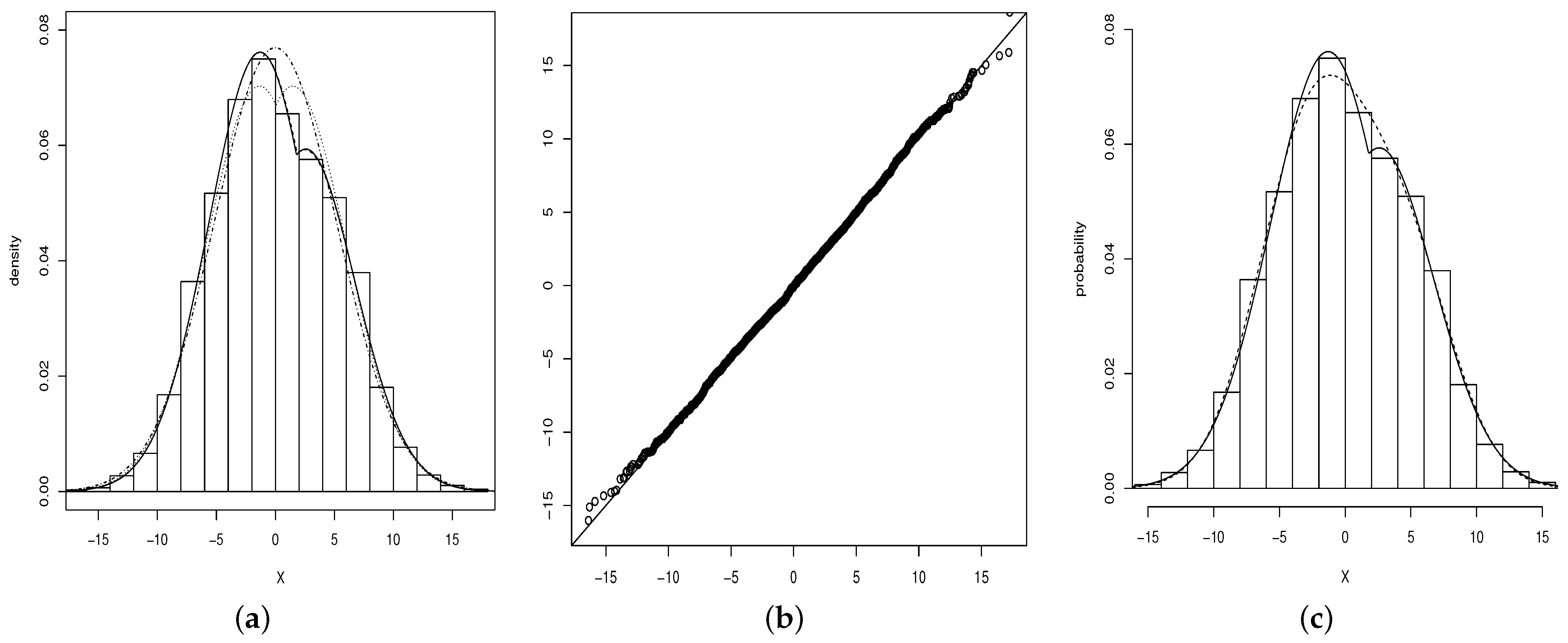
which is greater than the critical 5% chi-squared value, namely, ${\chi }_{1,95\%}^2=3.8414.$ Therefore, the SPN model seems to be a useful alternative for modeling the $nub$ data. Table 3 shows the estimated standard errors ML estimates (in parentheses) for the SN, TN, ETN and SPN models. In Figure 3, we can see that the ETN and SPN models fit quite well.

Table 3. Parameter estimates and standard errors for the SN, TN, ETN and SPN models.

Parameter	SN	TN	ETN	SPN
$\xi$	0.034 (0.032)	0.064 (0.074)	1.848 (0.123)	1.7951 (0.1290)
$\eta$	5.186 (0.067)	4.777 (0.069)	5.000 (0.062)	3.4988 (0.2395)
$\alpha$	−0.008 (1.216)	0.409 (0.102)	0.638 (0.131)	0.5112 (0.0540)
$\beta$	–	–	−0.417 (0.035)	−0.2839 (0.0316)
Log-likelihood	−11,793.47	−11,783.98	−11,774.47	−11,774.50
AIC	23,590.94	23,573.96	23,556.94	23,557.00
CAIC	23,605.45	23,595.73	23,567.45	23,567.51

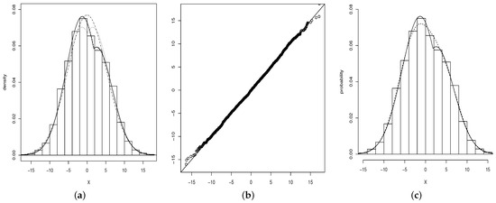
Figure 3. (a) Histogram for the variable $nub$. Densities adjusted by ML: TN (dotted line), SN (dotted and dashed line), ETN (dashed line) and SPN (solid line). (b) qq-plot for the variable $nub$. (c) SPN (solid line) and MN (dashed line).

It is evident that the fitting of the normal and SN models in this example is inadequate due to the asymmetric behavior and bimodality of the data. Thus, the TN, ETN and SPN models are adequate for fitting the variable $nub$, so it is more reasonable to contrast the SPN model with models by [16,17]. To compare the models, which are not nested, we use the AIC criterion [21], namely

$$AIC=-2\widehat{\ell }(·)+2k,$$

where k is the number of parameters of the model to consider. Furthermore, we consider the consistent AIC (CAIC) criterion, namely

$$CAIC=-2\widehat{\ell }(·)+(1+log\left(n\right))k,$$

where k is the number of parameters.

According to the AIC and CAIC criteria, the ETN and SPN models fit the variable $nub$ well, and much better than the TN model. Moreover, no significant differences are noted between the ETN and SPN models. Figure 3a shows clearly that the ETN and SPN models have the same degree of fit; note that the graph of the SPN model is superimposed on the ETN model. This shows the SPN model as a second alternative for modeling bimodal data. Figure 3b shows the qq-plot of the variable $nub$ for the SPN model.

Now we compare the SPN model with the mixture of the two normals model, which can be written as

$$f(x;{\mu }_1,{\sigma }_1,{\mu }_2,{\sigma }_2,p)=\frac{p}{{\sigma }_1}\varphi (x,{\mu }_1,{\sigma }_1)+\frac{1-p}{{\sigma }_2}\varphi (x;{\mu }_2,{\sigma }_2),$$

where $\varphi$ is the density of the standard normal distribution with parameters ${\mu }_j,{\sigma }_j$, $j=1,2$ and $0<p<1$. We denote the two-normals mixture model as MN$({\mu }_1,{\sigma }_1,{\mu }_2,{\sigma }_2,p)$.

The estimated model is

$$\mathrm{MN}(-2.389,4.106,4.649,3.698,0.6605)$$

with $AIC=23561.16\mathrm{and}CAIC=23569.67$. This model presents BIC and CAIC greater than those for the SPN model, so the SPN model fits the $nub$ data set better than the MN model. Figure 3c shows the estimated densities for the SPN and MN models.

5.2. Application 2

In this second application, we use the data available at http://lib.stat.cmu.edu/jasadata/laslett (accessed on 19 August 2021), which, according to their summary statistics (see Table 4), have appropriate characteristics to be modeled with distributions such as the one proposed in this research. A detailed description of these data can be found in the link above, where the roller surface roughness height is measured. In total, there are 1150 observations measured at 1-micron intervals along the roller drum.

Table 4. Summary statistics for the variable roller.

n	Mean	Variance	$\sqrt{{\mathit{\beta }}_1}$	${\mathit{\beta }}_2$
1150	3.535	0.650	−0.986	4.855

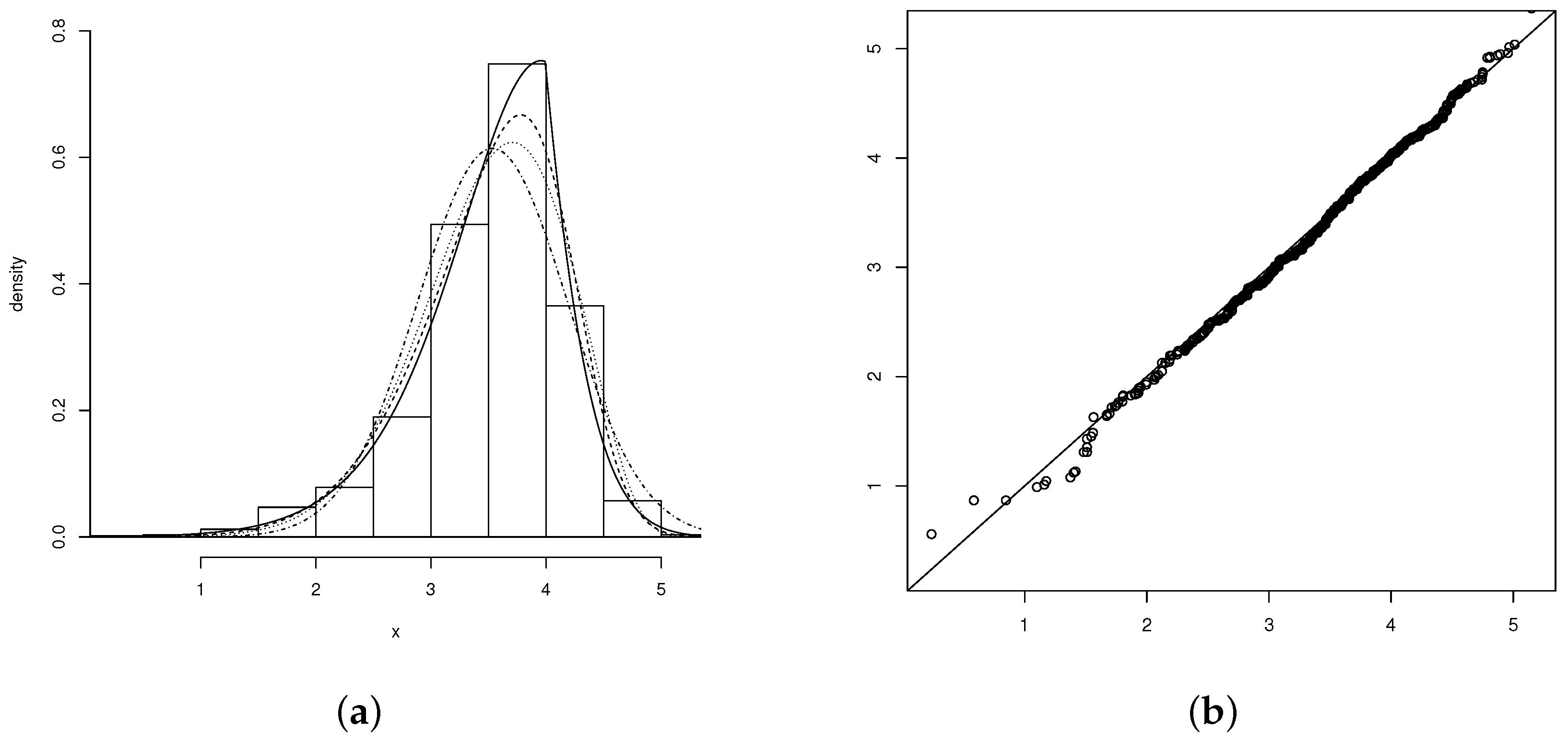
Hence, the PN, SN, and SPN models are fitted to the present data, and the MLE and standard errors (in parentheses) are calculated for each model studied (see Table 5). The results show the goodness of fit of the SPN model, which, compared to the other models, presents the best fit to the data. In addition, the plots of the fitted models are shown in Figure 4a, and the qq-plot for the SPN model is shown in Figure 4b.

Table 5. Parameter estimates (standard error) for the PN, SN and PSN distributions.

Parameter	PN	SN	SPN
$\xi$	4.5495 (0.0572)	4.2503 (0.0284)	3.9920 (0.0220)
$\eta$	0.1982 (0.0279)	0.9694 (0.0304)	3.4615 (0.9914)
$\alpha$	0.0479 (0.0156)	−2.7864 (0.2529)	6.5217 (2.1390)
$\beta$	–	–	−5.8626 (1.6601)
Log-likelihood	−1085.241	−1071.362	−1064.729
AIC	2176.482	2148.724	2137.458

Figure 4. (a) Histogram for the variable roller. Densities adjusted: PN$(4.5495,0.1982,0.0479)$ (dashed line), SN$(4.2503,0.9694,-2.7864)$ (dotted line) and SPN$(3.9920,3.4615,6.5217,-5.8626)$ (solid line). (b) qqplot for the variable roller.

In addition, a hypothesis test is performed to compare the normal model against the SPN model. Formally, we have the hypothesis

$$H_{01}:(\alpha ,\beta )=(1,0)\mathrm{versus}{H}_{11}:(\alpha ,\beta )\ne (1,0),$$

which can be tested using the statistic

$${\mathsf{\Lambda }}_1=\frac{{\ell }_N\left(\widehat{\mathbf{\theta }}\right)}{{\ell }_{\mathrm{SPN}}\left(\widehat{\mathbf{\theta }}\right)}.$$

After numerical evaluations, we obtain

$$-2log\left({\mathsf{\Lambda }}_1\right)=142.274,$$

which is greater than the 5% critical value of the Chi-squared distribution with one degree of freedom, namely ${\chi }_{1,95\%}^2=3.8414$.

According to the AIC criterion, the SPN model fits the roller data set better than the SN and PN models; i.e., the SPN model achieves satisfactory fitting of skewness and kurtosis, which are not adequately fitted by the previous models. A reason for the above situation can be explained because the skewness and kurtosis of the data analyzed are outside the permitted ranges for the SN ((−0.9953, 0.9953) and (3, 3.8692), respectively) and PN ((−0.6115, 0.9007) and (1.7170, 4.3556), respectively) models. This may be an indication that the SPN model has range of skewness and kurtosis greater than that of the SN and PN models.

6. Discussion

In this paper, we introduce a new family of continuous uni-/bimodal distributions. This family was generated based on power-symmetric and proportional hazards distributions. The SPN distribution, which is a particular case of this family, is studied in greater detail. The new family presented is a viable alternative for modeling asymmetric unimodal and bimodal data sets. Further specific conclusions are as follows, listed in order:

• The family of distributions presents flexibility in the modes of the base model, in both unimodal and bimodal cases;
• The parameters are estimated using the ML method; a simulation study for the maximum likelihood estimators indicates good parameter recovery;
• We show that the Fisher information matrix for the SPN distribution is nonsingular for the particular case of the normal distribution;
• In the first example, we contrasted the normal, SN and TN models. It is obvious that these models fail to capture the asymmetric bimodality of the data. In contrast, the ETN and SPN models are more suitable for fitting the distribution of the variable $nub$. In the second example we see that the normal, SN and PN models fail to adequately capture the high kurtosis of the variable roller. However, the SPN model appears to have more flexibility to fit this special feature.

References

- Azzalini, A. A class of distributions which includes the normal ones. Scand. J. Stat. 1985, 12, 171–178. [Google Scholar]
- Azzalini, A. Further results on a class of distributions which includes the normal ones. Statistica 1986, 46, 199–208. [Google Scholar]
- Henze, N. A probabilistic representation of the skew-normal distribution. Scand. J. Stat. 1986, 13, 271–275. [Google Scholar]
- Chiogna, M. Notes on Estimation Problems with Scalar Skew-Normal Distributions; Technical Report 15; Dept. Statistical Sciences, University of Padua: Padua, Italy, 1997. [Google Scholar]
- Pewsey, A. Problems of inference for Azzalini’s skew-normal distribution. J. Appl. Stat. 2000, 27, 859–870. [Google Scholar] [CrossRef]
- Venegas, O.; Sanhueza, A.I.; Gómez, H.W. An extension of the skew-generalized normal distribution and its derivation. Proyecc. J. Math. 2011, 30, 401–413. [Google Scholar] [CrossRef] [Green Version]
- Nadarajah, S.; Kotz, S. Skewed distributions generated by the normal kernel. Stat. Probab. Lett. 2003, 65, 269–277. [Google Scholar] [CrossRef]
- Gómez, H.W.; Venegas, O.; Bolfarine, H. Skew-symmetric distributions generated by the distribution function of the normal distribution. Environmetrics 2002, 18, 395–407. [Google Scholar] [CrossRef] [Green Version]
- Gómez-Déniz, E.; Arnold, B.C.; Sarabia, J.M.; Gómez, H.W. Properties and Applications of a New Family of Skew Distributions. Mathematics 2021, 9, 87. [Google Scholar] [CrossRef]
- Lehmann, E.L. The power of rank tests. Ann. Math. Stat. 1953, 24, 23–43. [Google Scholar] [CrossRef]
- Durrans, S.R. Distributions of fractional order statistics in hydrology. Water Resour. Res. 1992, 28, 1649–1655. [Google Scholar] [CrossRef]
- Eugene, N.; Lee, C.; Famoye, F. Beta-normal distribution and its applications. Commun. Stat. Theory Methods 2002, 31, 497–512. [Google Scholar] [CrossRef]
- Gupta, R.C.; Gupta, R.D. Generalized skew normal model. Test 2004, 12, 501–524. [Google Scholar] [CrossRef]
- Gupta, R.D.; Gupta, R.C. Analyzing skewed data by power normal model. Test 2008, 17, 197–210. [Google Scholar] [CrossRef]
- Pewsey, A.; Gómez, H.W.; Bolfarine, H. Likelihood-based inference for power distributions. Test 2012, 21, 775–789. [Google Scholar] [CrossRef]
- Kim, H.J. On a class of two-piece skew-normal distribution. Statistics 2005, 39, 537–553. [Google Scholar] [CrossRef]
- Arnold, B.C.; Gómez, H.W.; Salinas, H.S. On multiple constraint skewed models. Statistics 2009, 43, 279–293. [Google Scholar] [CrossRef]
- Cox, D. Regression models and life tables. J. R. Stat. Soc. Ser. B 1972, 34, 187–220. [Google Scholar] [CrossRef]
- Kalbfleisch, J.D.; Prentice, R.L. The Statistical Analysis of Failure Time Data, 2nd ed.; John Wiley and Sons: New York, NY, USA, 2002. [Google Scholar]
- Johnson, N.L.; Kotz, S.; Balakrishnan, N. Continuous Univariate Distributions, 2nd ed.; John Wiley and Sons: New York, NY, USA, 1994; pp. 53–54. [Google Scholar]
- Akaike, H. A new look at statistical model identification. IEEE Trans. Automat. Contr. 1974, 19, 716–723. [Google Scholar] [CrossRef]
Publisher’s Note: MDPI stays neutral with regard to jurisdictional claims in published maps and institutional affiliations. |
© 2022 by the authors. Licensee MDPI, Basel, Switzerland. This article is an open access article distributed under the terms and conditions of the Creative Commons Attribution (CC BY) license (https://creativecommons.org/licenses/by/4.0/).