Recent Advances in Robust Design for Accelerated Failure Time Models with Type I Censoring

Abstract

Many fields including clinical and manufacturing areas usually perform life-testing experiments and accelerated failure time models (AFT) play an essential role in these investigations. In these models the covariate causes an accelerant effect on the course of the event through the term named acceleration factor (AF). Despite the influence of this factor on the model, recent studies state that the form of AF is weakly or partially known in most real applications. In these cases, the classical optimal design theory may produce low efficient designs since they are highly model dependent. This work explores planning and techniques that can provide the best robust designs for AFT models with type I censoring when the form of the AF is misspecified, which is an issue little explored in the literature. Main idea is focused on considering the AF to vary over a neighbourhood of perturbation functions and assuming the mean square error matrix as the basis for measuring the design quality. A key result of this research was obtaining the asymptotic MSE matrix for type I censoring under the assumption of known variance regardless the selected failure time distribution. In order to illustrate the applicability of previous result to a study case, analytical characterizations and numerical approaches were developed to construct optimal robust designs under different contaminating scenarios for a failure time following a log-logistic distribution.

1. Introduction

Failure time data, also called time-to-event data or survival data, arise in many areas, including medical follow-up studies and reliability research. In these investigations often the event times are not always exactly observed because some units under observation may not experience the event of interest; that is, the data are censored and partial information from them is available. Different circumstances can produce different types of censoring. A right-censored failure time implies that the event is observed in a time greater than the last known survival time, either due to the end of the study or lose to follow-up. On the contrary, left censoring occurs when the actual survival time of an event is less than that observed. This kind of censoring occurs far less commonly than right censoring [1]. Another class of censored data is interval censoring, which is produced when the event is imprecisely experienced within an interval of time. The emphasis of this work will be on the analysis of data from a experiment which stops at a predetermined time, so that the survival time of any subjects remaining at this point are right-censored. The latter is also known as type I censoring.

Although the Cox’s Proportional Hazards (PH) model is commonly applied to analyze these data, it can generate severe problems when proportional hazards assumption is violated. Accelerated Failure Time (AFT) models have been considered as an alternative to PH models [2]. The AFT model has long been used in strength testing of materials, in which the units are exposed to higher than usual levels of stress to observe earlier failures. The type of distribution of the time-to-event variable has to be specified, and the objetive is to estimate the distribution of the failure time under usual conditions through the observed distribution of the failure time under accelerated conditions. Thus, AFT models provide a more appropriate modeling framework in many applications. A comprehensive and detailed exposition on accelerated failure testing can be found in [3].

Trial design is a primarily relevant stage in survival studies since practical limitations may involve time-consuming and expensive follow-ups [4]. In particular, planning decisions in AFT experiments are challenging due to the practical limitations of the study cases characterized by data censoring, non-normal distributions, non-linearity of the response and uncertainty about the AF form, to name a few. Thus, new design strategies are needed to overcome previous difficulties. Design issues in AFT experiments using the basis of Optimal Experimental Design (OED) theory were investigated for very rigid examples of particular distributions of the failure time (see [5,6,7] for Poisson, Weibull and Log-Normal distribution, respectively). Later, Müller [8] gave some theoretical results to construct local $D-$optimal designs considering the exponential distribution and based on equivalence theorem ideas. Rivas-López et al. [9] extended this theory obtaining a general expression of the information matrix for type I censoring regardless the assumed distribution. Recent real applications proposed sophisticated design plans fitted to the special features of their experimental applications [10,11]. Differently from OED techniques, other authors consider more rudimentary design strategies based on classical design [12], progressive censoring [13] or adaptative trials [14].

Robustness in the context of experimental design may be conceived from different approaches. Focusing on AFT models, robust designs were constructed to seek protection against misspecification of: (1) model parameter values, (2) the assumed distribution, and (3) the underlying stress–life relationship. The latter type of robustness is crucial for AFT models because the use level is often below the range of stress levels at which tests are conducted [15]. The interested reader is referred to [15] for an extensive review aimed at these three streams of research. Previous approaches have been addressed in the literature following two strategies mainly: (a) seeking a well design performance under different candidate models, and (b) assuming that the model form is only approximate and unknown departures, but controlled in some way, from the considered model may occur during the experiments. In the first vein, it should be noted the works due to Ginebra and Sen (1998) [16] and Pascual and Montepiedra (2002) [17]. The former computed minimax AFT designs when the parameter values are misspecified, whereas the latter discussed design issues comprising uncertainty on lifetime distribution. The main criticism of this strategy is that emphasizes on the design efficiency rather than on directly addressing the bias as a result of not choosing the “true” model [15]. On the other hand, there is a vast theory following (b), initiated by Box and Draper in 1959 [18] and latter extended in depth by Wiens [19,20,21] for other classes of models. In a survival context, this idea has been previously explored considering prediction and extrapolation problems for censored data [22] and the PH model [23]. As far as the authors know, the only existing work for AFT models under this perspective is due to Pascual (2006) [15]. In this work the author investigated the bias produced when a linear model is used to estimate life quantiles in AFT but the “true” one is quadratic.

Motivated by the gap in literature on the construction of robust designs for AFT models for a wider and not-predetermined class of possible departures from the considered model when AF is partially known, the present work arises. On the other hand, Nelson [24] holds that the Acceleration Factor (AF) is only partially known in most of practical cases, so that a better analysis would include the uncertainty in it. Under this framework, this work provides theory and methods for constructing robust designs when the AF is misspecified and the variance of the time-to-event variable is known. The approach adopted in this research lies in allowing the AF to vary over a neighborhood of possible departures of the considered form of the AF. The class of functions proposed by Huber [25] will be considered in this research for covering a sufficiently wide range of plausible alternate models and being the most commonly used in bias-robust literature. Construction strategies developed in this work were set for the example presented in [26], in which the log-logistic AFT model exhibited a better performance regarding goodness of fit compared with other life-testing models.

The next section contains the main features and the notation used for AFT models. The incorporation of the contaminating function in the AF and its implications over the design problem is also included in this section. The key result of this work is presented in Section 3: an analytical expression of the asymptotic mean squared error matrix for type I censoring which does not depend on the assumed distribution. In order to illustrate the applicability of previous result to a study case, optimal robust designs are constructed under different contaminating scenarios for the log-logistic distribution in Section 4. Finally, a brief discussion about the obtained results as well as the open lines of research are presented in Section 5.

2. Accelerated Failure Time Models

The AFT models look for the parameters of a probability distribution for a time-to-event variable, T, that is affected by some covariates $\mathbf{X}=(X_1,X_2,\cdots ,X_k)$ giving the conditions under which the experiment runs. Let $T_u$ be the random variable T observed in the usual levels of the covariates (for simplicity $X_i=0,\forall i=1,2,\cdots ,k$) following a distribution given by a baseline survival function, $S_u$. An AFT model is usually defined through this survival function,

$$S\left(t\right|\mathbf{x},\mathit{\theta })=S_u(t/AF(\mathbf{x},\mathit{\theta })),$$

where $AF(\mathbf{x},\mathit{\theta })$ is an acceleration factor, which speeds up the effect of the survival time in the survival function.

The AF is typically the exponential of a linear relationship,

$$AF(\mathbf{x},\mathit{\theta })=exp\left({\mathit{\theta }}^{\prime }\mathbf{x}\right).$$

Alternatively, the AFT model can be expressed through its log-linear form with respect to time as (see [27] for details)

$$log\left(T\right)=\mu +log\left(AF(\mathbf{x},\mathit{\theta })\right)+\sigma \epsilon =\mu +{\mathit{\theta }}^{\prime }\mathbf{x}+\sigma \epsilon$$

(1)

where $\mu \equiv E(log{T}_u)$ is the intercept, $\sigma \equiv Var(log{T}_u)$ is the scale parameter and $\epsilon$ is a random variable with a particular distribution with mean 0 and variance 1. It is assumed that the random variable T, for any values of the covariates $\mathbf{x}$, follows the same type of distribution than $T_u$.

The survival function of T expressed in terms of the survival function of $\epsilon$ is

$$S\left(t\right|\mathbf{x};\mu ,\mathit{\theta })=S_{\epsilon }\left(\frac{log\left(t\right)-\mu -{\mathit{\theta }}^{\prime }\mathbf{x}}{\sigma }\right)=S_{\epsilon }\left(z_t\right),$$

where it is defined

$$z_t=\frac{log\left(t\right)-\mu -{\mathit{\theta }}^{\prime }\mathbf{x}}{\sigma }.$$

From the above, the corresponding relationship between the Probability Density Functions (PDF) of T and $\epsilon$ is

$$f\left(t\right|\mathbf{x};\mu ,\mathit{\theta })=\frac{1}{\sigma t}·f_{\epsilon }\left(\frac{log\left(t\right)-\mu -{\mathit{\theta }}^{\prime }\mathbf{x}}{\sigma }\right)=\frac{1}{\sigma t}·f_{\epsilon }\left(z_t\right).$$

Members of the AFT model class include the Exponential, Weibull, Log-Logistic, Log-Normal and Gamma, among other distributions.

For interpretation purposes let us consider this class of models assuming an only dichotomous covariate X with two levels (e.g., labels of groups $x=1$ vs. $x=0$), then the expected ratio of the survival times for the two levels is $exp\left(\theta \right)$. Therefore, AFT models can be interpreted in terms of the rate of progression of a disease: a ratio above (under) 1 means that the time is accelerated (slowed down) by a constant factor.

2.1. Adding Uncertainty in the Aceleration Factor

If the experimenter’s choice on the acceleration factor is only approximate,

$$\eta (\mathbf{x},\mathit{\theta })\approx exp\left({\mathit{\theta }}^{\prime }\mathbf{x}\right),$$

and the “true” model is

$$\eta (\mathbf{x},\mathit{\theta })=exp\left({\mathit{\theta }}^{\prime }\mathbf{x}+\frac{\psi \left(\mathbf{x}\right)}{\sqrt{n}}\right)$$

for some unknown but ‘small’ function $\psi$ belonging to certain class of ‘contaminating’ functions $\Psi$, then the “true” log-linear model is

$$log\left(T\right)=\mu +{\mathit{\theta }}^{\prime }\mathbf{x}+\frac{\psi \left(\mathbf{x}\right)}{\sqrt{n}}+\sigma \epsilon =\mu +{\mathit{\theta }}^{\prime }\mathbf{x}+\sigma ·\left(\epsilon +\frac{\psi \left(\mathbf{x}\right)}{\sigma \sqrt{n}}\right)=\mu +{\mathit{\theta }}^{\prime }\mathbf{x}+\sigma \tilde{\epsilon },$$

(2)

with $\tilde{\epsilon }\sim \left({\mu }_{\tilde{\epsilon }}=\frac{\psi \left(\mathbf{x}\right)}{\sigma \sqrt{n}},{\sigma }_{\tilde{\epsilon }}=1\right)$ and n denotes the sample size. The term $\sqrt{n}$ is included joint with the contaminating function for an adequate asymptotic treatment of the bias as it will be seen later. Then, the PDF for the “true” model is

$$f\left(t\right|\mathbf{x};\mu ,\mathit{\theta })=\frac{1}{\sigma t}·f_{\epsilon }\left(\frac{log\left(t\right)-\mu -{\mathit{\theta }}^{\prime }\mathbf{x}}{\sigma }-\frac{\psi \left(\mathbf{x}\right)}{\sigma \sqrt{n}}\right)=\frac{1}{\sigma t}·f_{\tilde{\epsilon }}\left(z_t\right)$$

since $f_{\tilde{\epsilon }}\left(z_t\right)=f_{\epsilon }\left(z_t-\frac{\psi \left(\mathbf{x}\right)}{\sigma \sqrt{n}}\right)$.

Under this framework, the ’target’ parameter ${\mathit{\beta }}_0={\left({\mu }_0{\mathit{\theta }}_0\right)}^{\prime }$ is defined as

$${\mathit{\beta }}_0=arg\underset{\mathit{\beta }}{min}{\int }_{\chi }{\left(E\left[log\left(T\right)|x\right]{-log\left(T\right)|}_{\mathit{\beta }}\right)}^{2}d\mathit{x},$$

where $\mathit{\beta }={\left(\mu \mathit{\theta }\right)}^{\prime }$ and $\chi$ denotes the covariate design region. The above minimum condition requires to verify the following orthogonality condition:

$${\int }_{\chi }\mathit{h}\left(\mathit{x}\right)\psi \left(\mathit{x}\right)d\mathit{x}=\mathbf{0},$$

where $\mathit{h}\left(\mathit{x}\right)={(\mathrm{d}log\left(T\right)/\mathrm{d}\mathit{\beta }{|}_{\mathit{\beta }={\mathit{\beta }}_{\mathbf{0}}})}^{\prime }\mathit{\beta }$.

Two types of contaminating functions will be considered in this work:

$${\Psi }_1=\left\{\psi :\underset{x}{max}\left|\psi \left(x\right)\right|\le \tau ,{\int }_{\chi }\mathit{h}\left(\mathit{x}\right)\psi \left(\mathit{x}\right)d\mathit{x}=\mathbf{0},\psi \left(0\right)=0\right\},$$

and

$${\Psi }_2=\left\{\psi :{\int }_{\chi }{\psi }^2\left(\mathbf{x}\right)d\mathbf{x}\le {\eta }^2/n,{\int }_{\chi }\mathit{h}\left(\mathit{x}\right)\psi \left(\mathit{x}\right)d\mathit{x}=\mathbf{0},\psi \left(0\right)=0\right\},$$

where $\tau$ and $\eta$ are constants characterizing the neighborhood radio. The initial condition $\psi \left(0\right)=0$ is needed for satisfying that $AF\left(0\right)=1$. Although the class ${\Psi }_1$ is frequently found in several works [28,29,30], it has the disadvantage of being too ‘thin’ in the sense of limited robustness against realistic departures from the assumed model. Conversely, Huber [25] proposes a wider class of plausible alternative responses ${\Psi }_2$, which requires to consider continuous designs. Even though some example is stated in this work considering the class ${\Psi }_1$, our interest is in ${\Psi }_2$ for being the most commonly used class in bias-robust literature.

2.2. A Minimax Strategy to Construct Robust Designs

If model (1) is fitted but the “true” one is (2), the least squares estimator of the model parameters $\widehat{\mathit{\beta }}=(\widehat{\mu },\widehat{\mathit{\theta }})$ or the predicted response $\widehat{\mathit{Y}}\left(\mathit{x}\right)$ is biased, so that the Mean Squared Error (MSE) matrix of the estimates rather than variance becomes a suitable measure of design quality.

An objective function must be defined from the MSE matrix seeking to optimize some aspect of the sampling planning. The classical alphabetic optimality criteria are extended in robust designs replacing the variance-covariance matrix of the estimators by the MSE matrix. These optimality criteria are named loss functions in the bias-robust approach context. Two loss functions were selected in this research for covering both estimation purposes: model parameters and response. Thus, the D- and I-losses are defined as

$${\mathcal{L}}_D(\psi ,\xi )={det\mathrm{MSE}\left(\widehat{\mathit{\beta }}\right)}^{1/p}=\frac{{\sigma }^2}{n}{\left(\frac{1+{\mathit{b}}^{\prime }\left(\psi ,\xi \right){\left[\frac{{\sigma }^2}{n}\mathbf{M}\left(\xi \right)\right]}^{-1}\mathit{b}\left(\psi ,\xi \right)}{det\mathbf{M}\left(\xi \right)}\right)}^{1/p}$$

(3)

and

$${\mathcal{L}}_I(\psi ,\xi )={\int }_{\chi }\mathrm{MSE}\left(\widehat{Y}\left(\mathbf{x}\right)\right)d\mathbf{x}=\frac{{\sigma }^2}{n}Tr\left(A{M}^{-1}\left(\xi \right)\right)+b^{\prime }(\psi ,\xi )H\left(\xi \right)b(\psi ,\xi )+{\int }_{\chi }{\psi }^2\left(\mathbf{x}\right)d\mathbf{x}$$

(4)

respectively, where p is the number of model parameters,

$$\begin{array}{cc}\hfill A& ={\int }_{\chi }\mathit{h}\left(\mathit{x}\right)\mathit{h}{\left(\mathit{x}\right)}^{\prime }d\mathit{x},\hfill \\ \hfill M\left(\xi \right)& ={\int }_{\chi }\mathit{h}\left(\mathit{x}\right)\mathit{h}{\left(\mathit{x}\right)}^{\prime }d\xi \left(\mathit{x}\right),\hfill \\ \hfill H\left(\xi \right)& =M\left(\xi \right)A^{-1}M\left(\xi \right),\hfill \\ \hfill b(\psi ,\xi )& ={\int }_{\chi }\mathit{h}\left(\mathit{x}\right)\psi \left(\mathit{x}\right)d\xi \left(\mathit{x}\right).\hfill \end{array}$$

Our attention in this work is focused on considering both errors due to bias and sampling in the design problem, so that a minimax approach will be adopted. Therefore, it is defined a robust design or optimal robust design as one that minimizes the maximum of some scalar-valuated function of the MSE matrix of the estimates

$${\xi }^{*}=arg\underset{\xi }{min}\underset{\psi }{max}\mathcal{L}(\psi ,\xi ).$$

3. Asymptotic Mean Squared Error Matrix for Type I Censoring and Known Variance

Following [9] let us consider that all the individuals in the study are recruited at time 0 and that there is a follow-up until time d. The end of study is the only censoring considered here. We also assume $\sigma \equiv \mathrm{var}(logT)$ to be known.

Let $\delta \equiv 1_{\{T<d\}}$ be an indicator variable that is equal to 1 if the observation corresponds to an event and 0 if it corresponds to a right-censored observation. The log-likelihood function for model (1) and just one observation at value $\mathbf{x}$ is

$$\begin{array}{ccc}\hfill LL(\mu ,\mathit{\theta };t,\mathbf{x})& =& \delta log\left(f\right(t|\mathbf{x};\mu ,\mathit{\theta }))+(1-\delta )log(S\left(t\right|\mathbf{x};\mu ,\mathit{\theta }\left)\right)\hfill \\ \hfill & =& -\delta log\left(\sigma t\right)+\delta log\left(f_{\epsilon }\left(z_t\right)\right)+(1-\delta )log\left(S_{\epsilon }\left(z_t\right)\right)\hfill \end{array}$$

where $z_t=\frac{log\left(t\right)-\mu -{\mathit{\theta }}^{\prime }\mathbf{x}}{\sigma }$.

Let $\xi$ be an approximate design

$$\xi =\left\{\begin{array}{cccc}{\mathbf{x}}_1& {\mathbf{x}}_2& \cdots & {\mathbf{x}}_m\\ {\omega }_1& {\omega }_2& \cdots & {\omega }_m\end{array}\right\},0<{\omega }_i\le 1,\sum _{i=1}^m{\omega }_i=1$$

where ${\mathbf{x}}_1,{\mathbf{x}}_2,\cdots ,{\mathbf{x}}_m\in \chi (m\le n)$ are the distinct experimental values for the covariates and ${\omega }_i$ is the proportion of observations taken at ${\mathbf{x}}_i$.

In order to find the maximum likelihood estimator for the vector of model parameters assuming that the “true” model is (2), it is necessary to differentiate twice the log-likelihood, to compute its expectation and to analyze its limiting behavior. Thus the asymptotic information matrix of ${\mathit{\beta }}_0$ is

$$M\left(\xi \right)=M(\xi ,{\mathit{\beta }}_0)=\underset{n\to \infty }{lim}\frac{1}{n}\sum _{j=1}^n{I}^{\left(2\right)}({\mathit{\beta }}_0;t,{\mathbf{x}}_j)=\sum _{i=1}^m{\omega }_i{I}_{11}^{\left(2\right)}({\mathit{\beta }}_0;t,{\mathbf{x}}_i)\left(\begin{array}{cc}1& {\mathbf{x}}_i\\ {\mathbf{x}}_i& {\mathbf{x}}_i{\mathbf{x}}_i^{\prime }\end{array}\right),$$

with

$$\begin{array}{cc}\hfill I_{11}^{\left(2\right)}({\mathit{\beta }}_0;t,\mathit{x})& =E_{\left(2\right)}\left[-\frac{{\partial }^{2}LL(\mu ,\mathit{\theta };t,\mathbf{x})}{\partial {\mu }^2}\right]=\hfill \\ \hfill & =\frac{1}{{\sigma }^2}\left({\left[f_{\epsilon }^{\prime }\left(z\right)\right]}_{(-\infty )}+\frac{f_{\epsilon }{\left(z_d\right)}^2}{S_{\epsilon }\left(z_d\right)}+{\int }_{-\infty }^{z_d}\frac{f_{\epsilon }^{\prime }{\left(z\right)}^2}{f_{\epsilon }\left(z\right)}dz\right)+\hfill \\ \hfill & +\frac{\psi \left(\mathbf{x}\right)}{{\sigma }^3\sqrt{n}}\frac{1}{2}\left[\frac{f_{\epsilon }^{\prime }{\left(z_d\right)}^2}{f_{\epsilon }\left(z_d\right)}-{\left[\frac{f_{\epsilon }^{\prime }{\left(z\right)}^2}{f_{\epsilon }\left(z\right)}\right]}_{(-\infty )}-{\int }_{-\infty }^{z_d}\frac{f_{\epsilon }^{\prime }{\left(z\right)}^3}{f_{\epsilon }{\left(z\right)}^2}dz\right]+\hfill \\ \hfill & -\frac{\psi \left(\mathbf{x}\right)}{{\sigma }^3\sqrt{n}}\left(\frac{f_{\epsilon }^{\prime }\left(z_d\right)S_{\epsilon }\left(z_d\right)+f_{\epsilon }{\left(z_d\right)}^2}{S_{\epsilon }{\left(z_d\right)}^2}\right)\left({\left[f_{\epsilon }\left(z\right)\right]}_{(\infty )}-f_{\epsilon }\left(z_d\right)\right)+o\left(\frac{\psi \left(\mathbf{x}\right)}{\sigma \sqrt{n}}\right),\hfill \end{array}$$

where the two-term Taylor expansion of $f_{\tilde{\epsilon }}\left(z_t\right)$ was used. $f_{\epsilon }\left(z\right)$ must be of class ${\mathcal{C}}^2$ to satisfy the conditions given in Lemma 2.1 of [9]. Details for obtaining the previous formulae are shown in the Appendix A.

On the other hand, the asymptotic expectation of the score function at ${\mathit{\beta }}_0$ is

$$\begin{array}{cc}\hfill \tilde{b}(\xi ,\psi )& =\tilde{b}(\xi ,\psi ,{\mathit{\beta }}_0)=\frac{1}{\sqrt{n}}\underset{n\to \infty }{lim}\frac{1}{n}{E}_{\left(2\right)}\left[\sqrt{n}\sum _{j=1}^n\frac{\partial LL(\mathit{\beta };t,{\mathbf{x}}_j)}{\partial \mathit{\beta }}{|}_{{\mathit{\beta }}_0}\right]\hfill \\ \hfill & \\ \hfill & =\frac{1}{{\sigma }^2\sqrt{n}}\sum _{i=1}^m{\omega }_i\psi \left({\mathbf{x}}_i\right)\left[{\int }_{-\infty }^{z_d}\frac{f_{\epsilon }^{\prime }{\left(z\right)}^2}{f_{\epsilon }\left(z\right)}dz-\frac{f_{\epsilon }\left(z_d\right)}{S_{\epsilon }\left(z_d\right)}\left({\left[f_{\epsilon }\left(z\right)\right]}_{(\infty )}-f_{\epsilon }\left(z_d\right)\right)\right]\left(\begin{array}{c}1\\ {\mathbf{x}}_i\end{array}\right)\hfill \\ \hfill & \\ \hfill & :=\frac{1}{\sqrt{n}}b(\xi ,\psi ).\hfill \end{array}$$

Again, further explanation of above calculations is given in the Appendix A. Furthermore, the asymptotic variance–covariance matrix of the score function evaluated at ${\mathit{\beta }}_0$ is

$$C(\xi ,{\mathit{\beta }}_0)=\underset{n\to \infty }{lim}\frac{1}{n}\sum _{j=1}^{n}Cov\left[\frac{\partial LL(\mathit{\beta };t,{\mathbf{x}}_j)}{\partial \mathit{\beta }}{|}_{{\mathit{\beta }}_0}\right]=\sum _{i=1}^m{\omega }_i{I}_{11}^{\left(2\right)}({\mathit{\beta }}_0;t,{\mathbf{x}}_i)\left(\begin{array}{cc}1& {\mathbf{x}}_i\\ {\mathbf{x}}_i& {\mathbf{x}}_i{\mathbf{x}}_i^{\prime }\end{array}\right).$$

It should be noted that the asymptotic matrices $M\left(\xi \right)$ and $C\left(\xi \right)$ are identical and that the maximum likelihood estimate $\widehat{\mathit{\beta }}$ is a root of the score function $s\left(\mathit{\beta }\right)$. Therefore, using Taylor expansion of this function around ${\mathit{\beta }}_0$, the following is obtained

$$s\left(\mathit{\beta }\right)=s\left({\mathit{\beta }}_0\right)+s^{\prime }\left({\mathit{\beta }}_0\right)(\mathit{\beta }-{\mathit{\beta }}_0)+\dots \Rightarrow 0=s\left(\widehat{\mathit{\beta }}\right)\approx s\left({\mathit{\beta }}_0\right)+s^{\prime }\left({\mathit{\beta }}_0\right)(\widehat{\mathit{\beta }}-{\mathit{\beta }}_0).$$

Then $(\widehat{\mathit{\beta }}-{\mathit{\beta }}_0)\approx M^{-1}(\xi ,{\mathit{\beta }}_0)s\left({\mathit{\beta }}_0\right)$ and, since $\sqrt{n}s\left({\mathit{\beta }}_0\right)\sim AN(b(\xi ,\psi ),C\left(\xi \right)=M\left(\xi \right))$, the asymptotic distribution of $\sqrt{n}(\widehat{\mathit{\beta }}-{\mathit{\beta }}_0)$ is $AN\left(M^{-1}\left(\xi \right)b(\xi ,\psi ),M^{-1}\left(\xi \right)\right)$.

Finally, gathering previous results, it is obtained that the asymptotic MSE matrix is

$$\begin{array}{cc}\hfill MSE(\xi ,\psi )& =\left(M^{-1}\left(\xi \right)b(\xi ,\psi )\right)\left(M^{-1}\left(\xi \right)b^{\prime }(\xi ,\psi )\right)+M^{-1}\left(\xi \right)\hfill \\ \hfill & =M^{-1}\left(\xi \right)\left(b(\xi ,\psi )b^{\prime }(\xi ,\psi )+M\left(\xi \right)\right)M^{-1}\left(\xi \right).\hfill \end{array}$$

(5)

4. Log-Logistic Study Case

To illustrate previous results, let us assume that the variable T time-to-event to follow a log-logistic distribution with parameter $\sigma$ known. That is $T|\mathbf{x}\sim Log-Log\left[e^{\mu \left(\mathbf{x}\right)},{\displaystyle \frac{1}{\sigma }}\right]$ and variable $log\left(T\right|\mathbf{x})\sim Log[\mu \left(x\right),\sigma \left)\right]$.

In the non-contaminated case $T_u\sim Log-Log\left[e^{{\mu }_u},{\displaystyle \frac{1}{\sigma }}\right]$ and $log\left(T_u\right)\sim Log[{\mu }_u,\sigma ]$, so that $E[log\left(T_u\right)]={\mu }_u$ and $Var[log\left(T_u\right)]={\sigma }^2\frac{{\pi }^2}{3}={\sigma }_u$. Then, the corresponding log-linear form is

$$log\left(T\right|\mathbf{x})={\mu }_u+{\mathit{\theta }}^{\prime }\mathbf{x}+{\sigma }_u{\epsilon }^{\prime }={\mu }_u+{\mathit{\theta }}^{\prime }\mathbf{x}+\frac{\sigma \pi }{\sqrt{3}}{\epsilon }^{\prime }={\mu }_u+{\mathit{\theta }}^{\prime }\mathbf{x}+\sigma \epsilon$$

where ${\epsilon }^{\prime }\sim Log[0,\sqrt{3}/\pi ]$ and $\epsilon =\pi {\epsilon }^{\prime }/\sqrt{3}\sim Log[0,1]$. Consequently, $\epsilon$ follows a standard logistic distribution with PDF

$$f_{\epsilon }\left(z\right)=\frac{e^z}{{(1+e^z)}^2},-\infty <z<\infty$$

(6)

and survival function

$$S_{\epsilon }\left(z\right)=\frac{1}{1+e^z},-\infty <z<\infty ,$$

(7)

where $\sigma$ is again assumed known.

Finally, to obtain the MSE matrix (5) for this study case, it is necessary to compute

$$M\left(\xi \right)=M(\xi ,{\mathit{\beta }}_0)=\sum _{i=1}^m{\omega }_i{\mathcal{I}}_{11}^{\left(2\right)}({\mathit{\beta }}_0;t,{\mathbf{x}}_i)\left(\begin{array}{cc}1& {\mathbf{x}}_i\\ {\mathbf{x}}_i& {\mathbf{x}}_i{\mathbf{x}}_i^{\prime }\end{array}\right)$$

and

$$b(\xi ,\psi )=\sum _{i=1}^m{\omega }_i\psi \left({\mathbf{x}}_i\right){\mathcal{I}}_{11}^{\left(2\right)}({\mathit{\beta }}_0;t,{\mathbf{x}}_i)\left(\begin{array}{c}1\\ {\mathbf{x}}_i\end{array}\right),$$

where

$${\mathcal{I}}_{11}^{\left(2\right)}=\frac{1}{3{\sigma }^2}\left(1-S_{\epsilon }{\left(z_d\right)}^3\right)+o\left(\frac{\psi \left(\mathbf{x}\right)}{\sigma \sqrt{n}}\right)$$

by virtue of results given in Section 3 for Functions (6) and (7). Details for obtaining ${\mathcal{I}}_{11}^{\left(2\right)}$ are given in Appendix B.

4.1. Robust Desgins on ${\Psi }_1$

Let us consider a design region $\chi =\{0,1\}$ corresponding, for example, to two experimental treatments, A and B. Since there are two parameters to be optimally estimated in the model, both points 0 and 1 must be support points of the D-optimal robust design to be obtained. The following theorem provides an analytical solution of the minimax problem when the class of functions ${\Psi }_1$ is assumed.

Theorem 1.

Let $\psi \in {\Psi }_1$. The D-optimal robust design on $\chi =\{0,1\}$ allocates a proportion of ${\omega }^{*}$ observations at point $x=0$, where

$${\omega }^{*}=\frac{A(\theta ,\mu ,\sigma ,d)·(1+{\tau }^2)-B(\theta ,\mu ,\sigma )-\sqrt{\left(A^2(\theta ,\mu ,\sigma ,d)·(1+{\tau }^2)-{\tau }^{2}B(\theta ,\mu ,\sigma )\right)}}{{\tau }^2·(A(\theta ,\mu ,\sigma ,d)-B(\theta ,\mu ,\sigma ))}$$

with $A(\theta ,\mu ,\sigma ,d)=(e^{\frac{\theta +\mu }{\sigma }}+d^{1/\sigma }{)}^3,B(\theta ,\mu ,\sigma )=e^{3\frac{\theta +\mu }{\sigma }}$ and ${\omega }^{*}=1/2$ if $\tau =0$.

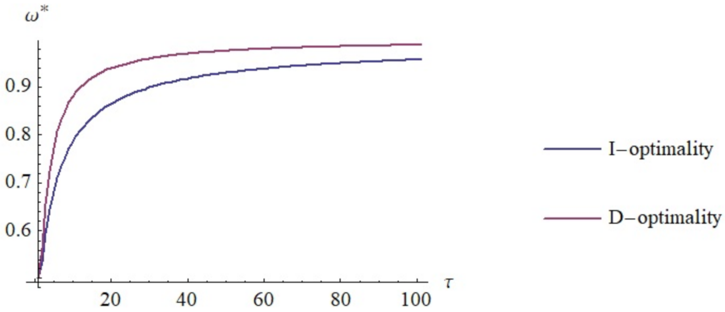
A proof of the above result is given in the Appendix C. Figure 1 shows the weight variation on $x=0$ as the neighborhood radio increases. From the graph it follows that the classical D-optimal design is obtained, which is equally weighted on all suport points, when the contamination is almost negligible. Nevertheless, the higher the neighborhood radio is, the more emphasis is placed on point $x=0$.

In the case of the I-optimality, it was not possible to find an analytical expression of the optimal weights. The solutions of the function to be maximized are the roots of a nine-order polynomial on $\omega$. For $\theta ,\mu ,\sigma ,d,\mathrm{and}\tau$ fixed, the numerical calculation of ${\omega }^{*}$ is straightforward. The same example as for D-optimization is also shown in the Figure 1 for I-optimality.

4.2. Robust Desgins on ${\Psi }_2$

The fact of assuming that T follows a log-logistic distribution implies that

$$M\left(\xi \right)={\int }_{\chi }\frac{1}{3{\sigma }^2}\left(1-S_{\epsilon }{\left(z_d\right)}^3\right)\left(\begin{array}{cc}1& \mathbf{x}\\ \mathbf{x}& \mathbf{x}{\mathbf{x}}^{\prime }\end{array}\right)d\xi \left(x\right),$$

where $h\left(\mathbf{x}\right)=\sqrt{a\left(\mathbf{x}\right)}g\left(x\right)$ being $a\left(\mathbf{x}\right)=\frac{1}{3{\sigma }^2}\left(1-S_{\epsilon }{\left(z_d\right)}^3\right)$ and $g\left(\mathit{x}\right)={\left(1\mathit{x}\right)}^{\prime }$. Matrices intervening in (3) and (4) are now

$$\begin{array}{ccc}\hfill A& =& {\int }_{\chi }a\left(\mathbf{x}\right)g\left(\mathbf{x}\right)g^{\prime }\left(\mathbf{x}\right)d\mathbf{x},\hfill \end{array}$$

(8)

$$\begin{array}{ccc}\hfill M\left(\xi \right)& =& {\int }_{\chi }a\left(\mathbf{x}\right)g\left(\mathbf{x}\right)g^{\prime }\left(\mathbf{x}\right)d\xi \left(\mathbf{x}\right),\hfill \end{array}$$

(9)

$$\begin{array}{ccc}\hfill H\left(\xi \right)& =& M\left(\xi \right)A^{-1}M\left(\xi \right),\hfill \end{array}$$

(10)

$$\begin{array}{ccc}\hfill b(\xi ,\psi )& =& {\int }_{\chi }a\left(\mathbf{x}\right)\psi \left(\mathbf{x}\right)g^{\prime }\left(\mathbf{x}\right)d\xi \left(\mathbf{x}\right).\hfill \end{array}$$

(11)

Let us define also

$$\begin{array}{ccc}\hfill K\left(\xi \right)& =& {\int }_{\chi }{a}^2\left(\mathbf{x}\right)g\left(\mathbf{x}\right)g^{\prime }\left(\mathbf{x}\right)d\xi \left(\mathbf{x}\right),\hfill \end{array}$$

(12)

$$\begin{array}{ccc}\hfill G\left(\xi \right)& =& K\left(\xi \right)-M\left(\xi \right)A^{-1}M\left(\xi \right),\hfill \end{array}$$

(13)

which will be useful later. In order to avoid singularity problems in matrices A and $M\left(\xi \right)$, let us assume that for each vector $\mathbf{v}\ne \mathbf{0}$, the set $\{\mathbf{x}\in \chi ,{\mathbf{v}}^{\prime }\mathbf{g}\left(\mathbf{x}\right)=0\}$ has Lebesgue measure zero [22].

Note that

(a)

$G\left(\xi \right)$ defined as above is positive semidefinite since

$$G={\int }_{\chi }\left[(a\left(\mathbf{x}\right)\mathbf{I}-M\left(\xi \right)A^{-1})\mathbf{g}\left(\mathbf{x}\right)\right]{\left[(a\left(\mathbf{x}\right)\mathbf{I}-M\left(\xi \right)A^{-1})\mathbf{g}\left(\mathbf{x}\right)\right]}^{\prime }d\xi \left(\mathbf{x}\right).$$

(b)

$a\left(\mathbf{x}\right)$ is a nonnegative function.

Theorem 2.

The maximums of ${\mathcal{L}}_D(\xi ,\psi )$ and ${\mathcal{L}}_I(\xi ,\psi )$ in ${\Psi }_2$ are

$$\begin{array}{ccc}\hfill \underset{\psi \in {\Psi }_2}{sup}{\mathcal{L}}_D(\xi ,\psi )& =& (1-\nu ){\left(\frac{1+\frac{\nu }{1-\nu }{\lambda }_{max}\left[M^{-1}\left(\xi \right)G\left(\xi \right)\right]}{detM\left(\xi \right)}\right)}^{1/p},\hfill \end{array}$$

(14)

$$\begin{array}{ccc}\hfill \underset{\psi \in {\Psi }_2}{sup}{\mathcal{L}}_I(\xi ,\psi )& =& (1-\nu )Tr\left(A{M}^{-1}\left(\xi \right)\right)+\nu {\lambda }_{max}\left[K\left(\xi \right)H^{-1}\left(\xi \right)\right],\hfill \end{array}$$

(15)

respectively, both attained at

$$\psi \left(\mathbf{x}\right)=\frac{\eta }{\sqrt{n}}{\mathbf{g}}^{\prime }\left(\mathbf{x}\right)\{a\left(\mathbf{x}\right)I-A^{-1}M\left(\xi \right)\}{\mathbf{c}}_{{\lambda }_{max}}$$

where ${\mathbf{c}}_{{\lambda }_{max}}$ is the normalized eigenvector corresponding to the maximum eigenvalue, ${\lambda }_{max}$, of the matrices $M^{-1}\left(\xi \right)G\left(\xi \right)$ and $K\left(\xi \right)H^{-1}\left(\xi \right)$, respectively. The constant

$$\nu ={\displaystyle \frac{{\eta }^2}{{\sigma }^2+{\eta }^2}}\in [0,1]$$

is defined representing the relative importance, to the experimenter, of errors due to bias rather than to variance.

An outline of the proof is given in Appendix D. Then, the initial minimax problem for both D- and I-optimality criteria has become one of finding a design that minimizes (14) and (15), respectively. To this end, and since practitioners require exact designs to implement their experiments, we propose the following strategy:

• To distretize the design region $\chi$.
• To consider n-point exact designs $\xi =\left\{\begin{array}{ccc}{x}_1& ...& x_n\\ {\omega }_1& ...& {\omega }_n\end{array}\right\}$, $x_i\in \chi$ not necessarily different and being ${\omega }_i$’s integer multiples of $1/n$.
• To define the discrete version of matrices (8)–(12) replacing ∫ by ∑ properly.
• To use an heuristic algorithm to numerically minimize (14) and (15) according to Theorem 2.

In order to illustrate the previous results, let us consider the real application proposed by Qi (2009) [26]. Here the author considered a randomized placebo-controlled trial to prevent tuberculosis in Ugandan adults infected with HIV. Log-logistic distribution exhibited the best fit in this studio. Let $x\in \chi =[0,1]$ be the covariate (dose) to be designed and let $d=3,\sigma =0.71,\mu =-2.97,\mathrm{and}\theta =0.1$ be the selected nominal values as in [26]. An heuristic algorithm is required for the loss minimization according to step 4. In this work, a Genetic Algorithm (GA) similar to that presented in García-Camacha et al. (2020) [31] will be used for this purpose.

Table 1. 2-point D-optimal robust designs computed for the log-logistic model.

$\mathit{\nu }$	D-Optimal Robust Designs
$\begin{array}{c}0.01\\ 0.3\\ 0.5\\ 0.7\end{array}$	${\xi }_D^{*}=\left\{\begin{array}{cc}0& 1\\ 0.5& 0.5\end{array}\right\}$
0.91	${\xi }_D^{*}=\left\{\begin{array}{cc}0.34& 0.99\\ 0.5& 0.5\end{array}\right\}=\left\{\begin{array}{cc}0.01& 0.66\\ 0.5& 0.5\end{array}\right\}$

,

Table 2. 10-point D-optimal robust designs computed for the log-logistic model.

$\mathit{\nu }$	D-Optimal Robust Designs
0.01	${\xi }_D^{*}=\left\{\begin{array}{cccccc}0& 0.01& 0.02& 0.98& 0.99& 1\\ 0.2& 0.2& 0.1& 0.1& 0.2& 0.2\end{array}\right\}$
$\begin{array}{c}0.3\\ 0.5\end{array}$	${\xi }_D^{*}=\left\{\begin{array}{cccccccccc}0& 0.01& 0.02& 0.03& 0.04& 0.96& 0.97& 0.98& 0.99& 1\\ 0.1& 0.1& 0.1& 0.1& 0.1& 0.1& 0.1& 0.1& 0.1& 0.1\end{array}\right\}$
0.7	${\xi }_D^{*}=\left\{\begin{array}{cccccccccc}0& 0.08& 0.54& 0.60& 0.73& 0.76& 0.86& 0.93& 0.96& 1\\ 0.1& 0.1& 0.1& 0.1& 0.1& 0.1& 0.1& 0.1& 0.1& 0.1\end{array}\right\}$
0.91	${\xi }_D^{*}=\left\{\begin{array}{cccccccccc}0.39& 0.43& 0.60& 0.62& 0.67& 0.70& 0.79& 0.83& 0.94& 0.96\\ 0.1& 0.1& 0.1& 0.1& 0.1& 0.1& 0.1& 0.1& 0.1& 0.1\end{array}\right\}$

,

Table 3. 2-point I-optimal robust designs computed for the log-logistic model.

$\mathit{\nu }$	I-Optimal Robust Designs
$\begin{array}{c}0.01\\ 0.3\\ 0.5\\ 0.7\\ 0.91\end{array}$	${\xi }_I^{*}=\left\{\begin{array}{cc}0& 1\\ 0.5& 0.5\end{array}\right\}$

and

Table 4. 10-point I-optimal robust designs computed for the log-logistic model.

$\mathit{\nu }$	I-Optimal Robust Designs
$\begin{array}{c}0.01\\ 0.3\\ 0.5\\ 0.7\\ 0.91\end{array}$	${\xi }_I^{*}=\left\{\begin{array}{cccccccccc}0& 0.01& 0.02& 0.03& 0.04& 0.96& 0.97& 0.98& 0.99& 1\\ 0.1& 0.1& 0.1& 0.1& 0.1& 0.1& 0.1& 0.1& 0.1& 0.1\end{array}\right\}$

collect the D- and I-optimal robust designs with 2 and 10 points, respectively. It is important to note that the D-optimal robust design achieved when the variance is almost ignored ($\nu =0.91$) is not unique. On the other hand, the achieved I-optimal robust design remains unchanged regardless the certainty that the experimenter has about model adequacy. A similar phenomenon is documented in the context of mixture designs [32] as both terms involved in (4) are proportionals. This result is a very desirable design property for seeking robustness.

The classical alphabetic optimality criteria, based on variance alone, have the appealing property of being convex functionals of the design. This allows for the establishment of equivalence theorems, by which a design is optimal if it satisfies first-order conditions. When bias is incorporated into the loss, this convexity is lost and so the first-order conditions, necessary for optimality, cannot be proved to be sufficient [33]. Therefore, the only way to validate the obtained designs in this work is to compare with those obtained in the literature (if available). In this regard, the classical 2-point D-optimal design obtained in this work is the same as that obtained in [9] (case $\nu =0$).

Table 5. Number of iterations needed for achieving the D-optimal robust designs computed in Table 1 and Table 2, their corresponding loss function values and efficiencies.

$\mathit{\nu }$	No. It (2p)	D-Loss (2p)	Efficiency	No. It (10p)	D-Loss (10p)	Efficiency
0.01	1037	2.2989	-	1744	3.04	-
0.3	1008	1.961	-	1239	1.903	99.05
0.5	1436	1.237	-	1270	1.002	96.37
0.7	1080	0.4338	-	1125	0.001823	0.31
0.91	1061	0.01426	3.42	1617	0.00103	0.22

and

Table 6. Number of iterations needed for achieving the I-optimal robust designs computed in Table 3 and Table 4, and their corresponding loss function values.

$\mathit{\nu }$	No. It (2p)	I-Loss (2p)	No. It (10p)	I-Loss (10p)
0.01	1063	2.011	1916	2.05
0.3	1120	1.569	1543	1.479
0.5	1015	1.263	1184	1.085
0.7	1103	0.9579	1284	0.6909
0.91	1006	0.6374	1328	0.2773

show the computational cost, measured in terms of number of the algorithm iterations, and the obtained loss function values for D- and I-optimal robust designs.

In order to show the benefits of the obtained robust designs ($\nu >0$) versus designs calculated using the classical optimal design theory ($\nu =0$), efficiencies were calculated as ${\displaystyle \frac{los{s}_{\nu }\left({\xi }_{\nu }^{*}\right)}{los{s}_{\nu }\left({\xi }_{\nu =0}^{*}\right)}}\times 100$. These efficiencies range from 0 to 1, so that values close to 0 indicate that classical design is not robust at all, while a value of 1 means the opposite case. Note that for study cases in which the robust design coincides with the classical one, calculating the efficiency is meaningless (which occurs for the I-optimal robust designs and for $\nu \le 0.7$ in the case of D-optimality and two-point designs). When the knowledge of model is almost non-existent or many deviations of it occur during experiments ($\nu =0.91$), two-point classical D-optimal design is $3.42\%$ efficient compared with the proposed ones in Table 1. Efficiencies of ten-point classical D-optimal design compared with the obtained robust designs are shown in Table 5.

5. Discussion

Accelerated failure time models have been widely used in industrial processes, but nowadays they are becoming popular in many other fields, including medical research. This fact is not only due to their relaxed conditions compared with proportional hazard models, but also due to the easy interpretation of the effects for applicability purposes [9]. The main feature characterizing this type of models is that the covariates have a multiplicative effect which accelerates/decelerates the survival. Nevertheless, practitioners rarely know the exact form of the acceleration factor [24], which is something necessary to obtain optimal designs, strongly dependent of the model.

In this work we provide robust designs against departures from the assumed acceleration factor. To this end, a space of contaminating functions was considered, and the mean square error matrix was established as the basis for measuring the design quality. A key result of this research was obtaining the asymptotic expression of this matrix for type I censoring and known variance. This expression is general in the sense that it does not depend on the selected failure time distribution.

Several study cases were analysed considering the log-logistic distribution to illustrate the previous result. First example comprises a bounded contaminating space and a placebo-treatment type design region. Theoretical support is provided for constructing the D-optimal robust design, whereas the I-optimal problem can be only solved numerically. Two types of contaminating functions are considered in this work. The maximization problem over these classes of functions is theoretically solved and a construction strategy similar to [31] for computing the D- and I-robust designs is used when the contaminating funcions are a $L_2$-type neighbourhood.

Methodology used for calculating the obtained designs was confirmed when there was available information in the literature. Note that there is a lack of equivalence theorems since convexity might be violated under bias-robust approach [33]. D-optimal robust designs tend to be equally weighted on the extremes when the model form is either known or almost known, whereas the allocation is more random when bias emphasizes. This latter is a quite common result in robust design [34]. It seems logical to think that an adequate strategy to seek protection against the misspecification total or quasi total of the model is not favoring any design region. On the other hand, the achieved I-optimal robust design remains unchanged regardless the certainty that the experimenter has about model adequacy. This is a very desirable design property for seeking robustness.

As we mentioned before, peculiarities of real experiments lead to different censoring. Some authors warn of the risks of addressing data as right-censored when interval censoring occurs [35,36]. This may lead to biased estimates or underestimates of the “true” error variance or the survival itself. So censoring mechanisms can be quite complicated and thus special methods are necessary for their appropriate treatment. Further research must be aimed at this important issue. New alternatives for interval censored data under this bias-robust approach proposed in this work are being explored.

References

- Collett, D. Modelling Survival Data in Medical Research; CRC Press: Boca Raton, FL, USA, 2015. [Google Scholar]
- Wei, L.J. The accelerated failure time model: A useful alternative to the cox regression model in survival analysis. Stat. Med. 1992, 11, 1871–1879. [Google Scholar] [CrossRef] [PubMed]
- Escobar, L.A.; Meeker, W.Q. A Review of Accelerated Test Models. Stat. Sci. 2006, 21, 552–577. [Google Scholar] [CrossRef] [Green Version]
- Gökkuş, Z.; Alakuş, K.; Bilen, S. USE of group sequential test methods in the survival analysis in aquaculture. Aquaculture 2020, 515, 734568. [Google Scholar] [CrossRef]
- Bai, D.; Chung, S. An optimal design of accelerated life test for exponential distribution. Reliab. Eng. Syst. Saf. 1991, 31, 57–64. [Google Scholar] [CrossRef]
- Ahmad, N.; Islam, A.; Salam, A. Analysis of optimal accelerated life test plans for periodic inspection: The case of exponentiated Weibull failure model. Int. J. Qual. Reliab. Manag. 2006, 23, 1019–1046. [Google Scholar] [CrossRef]
- Das, R.N.; Lin, D.K. On D-optimal robust designs for lifetime improvement experiments. J. Stat. Plan. Inference 2011, 141, 3753–3759. [Google Scholar] [CrossRef]
- Müller, C.H. D-Optimal Designs for Lifetime Experiments with Exponential Distribution and Censoring. In mODa 10—Advances in Model-Oriented Design and Analysis; Ucinski, D., Atkinson, A.C., Patan, M., Eds.; Springer International Publishing: Heidelberg, Germany, 2013; pp. 179–186. [Google Scholar] [CrossRef]
- Rivas-López, M.J.; López-Fidalgo, J.; Campo, R.d. Optimal experimental designs for accelerated failure time with Type I and random censoring. Biom. J. 2014, 56, 819–837. [Google Scholar] [CrossRef]
- Rivas-López, M.; Yu, R.; López-Fidalgo, J.; Ruiz, G. Optimal experimental design on the loading frequency for a probabilistic fatigue model for plain and fibre-reinforced concrete. Comput. Stat. Data Anal. 2017, 113, 363–374. [Google Scholar] [CrossRef] [Green Version]
- Mariñas Collado, I.; Rivas-López, M.J.; Rodríguez-Díaz, J.M.; Santos-Martín, M.T. A New Compromise Design Plan for Accelerated Failure Time Models with Temperature as an Acceleration Factor. Mathematics 2021, 9, 836. [Google Scholar] [CrossRef]
- Liang, T.; Chen, L.S.; Yang, M.C. Efficient Bayesian sampling plans for exponential distributions with random censoring. J. Stat. Plan. Inference 2012, 142, 537–551. [Google Scholar] [CrossRef]
- Park, S.; Ng, H.K.T. Missing information and an optimal one-step plan in a Type II progressive censoring scheme. Stat. Probab. Lett. 2012, 82, 396–402. [Google Scholar] [CrossRef]
- Ryeznik, Y.; Sverdlov, O.; Hooker, A.C. Adaptive optimal designs for dose-finding studies with time-to-event outcomes. AAPS J. 2018, 20, 1–12. [Google Scholar] [CrossRef] [PubMed] [Green Version]
- Pascual, F.G. Accelerated Life Test Plans Robust to Misspecification of the Stress—Life Relationship. Technometrics 2006, 48, 11–25. [Google Scholar] [CrossRef]
- Ginebra, J.; Sen, A. Minimax approach to accelerated life tests. IEEE Trans. Reliab. 1998, 47, 261–267. [Google Scholar] [CrossRef]
- Pascual, F.; Montepiedra, G. On minimax designs when there are two candidate models. J. Stat. Comput. Simul. 2002, 72, 841–862. [Google Scholar] [CrossRef]
- Box, G.E.P.; Draper, N.R. A Basis for the Selection of a Response Surface Design. J. Am. Stat. Assoc. 1959, 54, 622–654. [Google Scholar] [CrossRef]
- Wiens, D.P. Minimax designs for approximately linear regression. J. Stat. Plan. Inference 1992, 31, 353–371. [Google Scholar] [CrossRef]
- Wiens, D.P. Designs for approximately linear regression: Maximizing the minimum coverage probability of confidence ellipsoids. Can. J. Stat. 1993, 21, 59–70. [Google Scholar] [CrossRef]
- Wiens, D.P. Robust designs for approximately linear regression: M-estimated parameters. J. Stat. Plan. Inference 1994, 40, 135–160. [Google Scholar] [CrossRef]
- Xu, X. Robust prediction and extrapolation designs for censored data. J. Stat. Plan. Inference 2009, 139, 486–502. [Google Scholar] [CrossRef] [Green Version]
- Konstantinou, M.; Biedermann, S.; Kimber, A. Model robust designs for survival trials. Comput. Stat. Data Anal. 2017, 113, 239–250. [Google Scholar] [CrossRef] [Green Version]
- Nelson, W.B. Accelerated Testing: Statistical Models, Test Plans, and Data Analysis; John Wiley & Sons: Hoboken, NJ, USA, 2009; Volume 344. [Google Scholar]
- Huber, P.J. Robustness and designs. In A Survey of Statistical Design and Linear Models; North Holland: Amsterdam, The Netherlands, 1975; pp. 287–303. [Google Scholar]
- Qi, J. Comparison of Proportional Hazards and Accelerated Failure Time Models. Ph.D. Thesis, Department of Mathematics and Statistics, University of Saskatchewan, Saskatoon, SK, Canada, 2009. [Google Scholar]
- Orbe, J.; Núñez-Antón, V. Alternative approaches to study lifetime data under different scenarios: From the PH to the modified semiparametric AFT model. Comput. Stat. Data Anal. 2006, 50, 1565–1582. [Google Scholar] [CrossRef]
- Marcus, M.B.; Sacks, J. Robust designs for regression problems. In Statistical Decision Theory and Related Topics; Elsevier: Amsterdam, The Netherlands, 1977; pp. 245–268. [Google Scholar]
- Pesotchinsky, L. Optimal robust designs: Linear regression in Rk. Ann. Stat. 1982, 10, 511–525. [Google Scholar] [CrossRef]
- Li, K.C. Robust regression designs when the design space consists of finitely many points. Ann. Stat. 1984, 12, 269–282. [Google Scholar] [CrossRef]
- García-Camacha Gutiérrez, I.; Martín Martín, R.; Sanz Argent, J. Optimal-robust selection of a fuel surrogate for homogeneous charge compression ignition modeling. PLoS ONE 2020, 15, e0234963. [Google Scholar] [CrossRef] [PubMed]
- García-Camacha Gutiérrez, I. Diseño Óptimo de Experimentos para Modelos de Mezclas Aplicados en la Ingeniería y las Ciencias Experimentales. Ph.D. Thesis, University of Castilla-La Mancha, Ciudad Real, Spain, 2017. Available online: http://hdl.handle.net/10578/16595 (accessed on 28 September 2021).
- Wiens, D.P. I-robust and D-robust designs on a finite design space. Stat. Comput. 2018, 28, 241–258. [Google Scholar] [CrossRef]
- Kong, L.; Wiens, D.P. Model-Robust Designs for Quantile Regression. J. Am. Stat. Assoc. 2015, 110, 233–245. [Google Scholar] [CrossRef]
- Rücker, G.; Messerer, D. Remission duration: An example of interval-censored observations. Stat. Med. 1988, 7, 1139–1145. [Google Scholar] [CrossRef]
- Law, C.; Brookmeyer, R. Effects of mid-point imputation on the analysis of doubly censored data. Stat. Med. 1992, 11, 1569–1578. [Google Scholar] [CrossRef]
Publisher’s Note: MDPI stays neutral with regard to jurisdictional claims in published maps and institutional affiliations. |
© 2022 by the authors. Licensee MDPI, Basel, Switzerland. This article is an open access article distributed under the terms and conditions of the Creative Commons Attribution (CC BY) license (https://creativecommons.org/licenses/by/4.0/).