Two-Field Weak Solutions for a Class of Contact Models

Abstract

Two contact models are considered, with the behavior of the materials being described by a constitutive law governed by the subdifferential of a convex map. We deliver variational formulations based on the theory of bipotentials. In this approach, the unknowns are pairs consisting of the displacement field and the Cauchy stress tensor. The two-field weak solutions are sought into product spaces involving variable convex sets. Both models lead to variational systems which can be cast in an abstract setting. After delivering some abstract results, we apply them in order to study the weak solvability of the mechanical models as well as the data dependence of the weak solutions.

1. Introduction

The necessity of a better approximation of the solutions of physical models by using numerical methods determined the consideration of additional fields in the variational setup, leading to multifield variational formulations; see, e.g., [1,2,3] and the references therein for some variational approaches based on the saddle point theory. When the constitutive laws present in the description of the models are governed by possibly set-valued operators, then a possible approach is the one governed by bipotentials (see, e.g., [4,5,6,7]); for other relevant works devoted to bipotentials and their applicability in mechanics, we refer, for instance, to [8,9,10,11].

The present paper is a new contribution to the variational formulations governed by bipotentials in solid mechanics, addressing models whose constitutive laws are described by means of the subdifferential of a convex map. Two contact models are under our attention. The first model involves the Winkler condition on the contact zone, with such a boundary condition having extensive applications in civil engineering, e.g., [12]. The second model involves a regularized Coulomb friction law; see, e.g., [13] (pp. 107–110) and the references therein for details. We emphasize that the second model is strongly nonlinear—the nonlinearity arising not only from the constitutive law, but also from the friction law.

We focus on the existence and the uniqueness of the weak solutions and also on their dependence on the data.

Due to the separability property of the bipotential which is involved, the variational formulations we deliver can be cast in an abstract variational system of the form below

$$\begin{array}{cc}J\left(v\right)-J\left(u\right)+\widehat{g}j(u,v-u)& \ge {(f,v-u)}_X\mathrm{for} \mathrm{all} v\in X\end{array}$$

(1)

$$\begin{array}{cc}{J}^{*}\left(\mu \right)-J^{*}\left(\sigma \right)& \ge 0\mathrm{for} \mathrm{all} \mu \in K_j(u;f,\widehat{g})\subset Y.\end{array}$$

(2)

The unknown is the pair $(u,\sigma )\in X\times K_j(u;f,\widehat{g})$ for given $J:X\to \mathbb{R},$ $J^{*}:Y\to \mathbb{R},$ $j:X\times X\to \mathbb{R},$ $f\in X$ and $\widehat{g}>0.$ It is worth emphasizing that the second variational inequality is written on a set $K_j(u;f,\widehat{g})$ which depends on the first component of the pair solution, u. In order to investigate the existence and the uniqueness of the solution of this abstract system, we use elements of convex analysis, a crucial role being played by a minimization argument. On the other hand, by using the weak topology and a Mosco convergence technique, we investigate the continuity of the solution operator

$$S:X\times \mathbb{R}\to X\times Y,S(f,\widehat{g})=(u,\sigma ),$$

(3)

proving its demicontinuity, i.e., we prove that if $(f_n,{\widehat{g}}_n)\to (f,\widehat{g})$ in $X\times \mathbb{R}$ as $n\to \infty$ then $(u_n,{\sigma }_n)\rightharpoonup (u,\sigma )$ in $X\times Y$ as $n\to \infty .$ Afterward, we apply the abstract results in order to study the mechanical models under consideration.

This work can be seen as a continuation of [7]. The model studied in [7] can be revisited by applying the abstract results obtained in the present paper.

It is worth mentioning that the subdifferential of convex maps is present not only in solid mechanics but also in many other fields of mathematical physics. The subdifferential of convex maps is widely used especially in those cases in which the materials have an extremely complex intrinsic structure, such as complex fluids and/or magnetorheological fluids; see, e.g., [14,15,16,17].

The rest of the paper is structured as follows: In Section 2, we indicate some preliminaries, including basic facts of convex analysis. In Section 3, we present two mechanical models and their corresponding two-field weak formulations via bipotentials. Section 4 is devoted to some abstract results which are applied in Section 5 in order to obtain existence and uniqueness results as well as some properties of the weak solutions. Finally, Section 6 is devoted to conclusions and perspectives.

2. Preliminaries

For the convenience of the reader, we present in this section some notations, preliminary results from convex analysis and definitions of some mathematical concepts that are used throughout the paper. Everywhere in the present work, by the abbreviation a.e., we mean “almost everywhere”. Throughout this paper, ${\mathbb{S}}^3$ denotes the space of second-order symmetric tensors on ${\mathbb{R}}^3.$ Every field in ${\mathbb{R}}^3$ or ${\mathbb{S}}^3$ is typeset in boldface. By · and :, we denote the inner product on ${\mathbb{R}}^3$ and ${\mathbb{S}}^3$, respectively, while by means of the notation $\parallel ·\parallel$ and ${\parallel ·\parallel }_{{\mathbb{S}}^3}$, we denote the Euclidean norm on ${\mathbb{R}}^3$ and ${\mathbb{S}}^3$, respectively.

Let $\Omega \subset {\mathbb{R}}^3$ be a bounded domain with smooth enough boundary $\Gamma$. We begin with the description of the spaces that are used in this paper:

• $L^2{(\Omega )}^{3\times 3}=\{\mathbf{\mu }=\left({\mu }_{ij}\right):{\mu }_{ij}\in L^2(\Omega )\mathrm{for} \mathrm{all} i,j\in \{1,2,3\}\}$ is a Hilbert space endowed with the inner product ${(·,·)}_{L^2{(\Omega )}^{3\times 3}},$ ${(\mathbf{\mu },\mathbf{\tau })}_{L^2{(\Omega )}^{3\times 3}}={\int }_{\Omega }{\sum }_{i,j=1}^3{\mu }_{ij}\left(x\right){\tau }_{ij}\left(x\right)dx.$
• $L_s^2{(\Omega )}^{3\times 3}=\{\mathbf{\mu }=\left({\mu }_{ij}\right):{\mu }_{ij}\in L^2(\Omega ),{\mu }_{ij}={\mu }_{ji}\mathrm{for} \mathrm{all} i,j\in \{1,2,3\}\}$ is a Hilbert space endowed with the inner product ${(·,·)}_{L_s^2{(\Omega )}^{3\times 3}},$ ${(\mathbf{\mu },\mathbf{\tau })}_{L_s^2{(\Omega )}^{3\times 3}}={(\mathbf{\mu },\mathbf{\tau })}_{L^2{(\Omega )}^{3\times 3}}.$
• $V=\{\mathit{v}\in H^1{(\Omega )}^3:\mathbf{\gamma }\mathit{v}=\mathbf{0} \mathrm{a.e.} \mathrm{on} {\Gamma }_1\}$, with ${\Gamma }_1\subset \Gamma$ such that $meas\left({\Gamma }_1\right)>0,$ is a Hilbert space endowed with the inner product ${(·,·)}_V:V\times V\to \mathbb{R},{(u,v)}_V={(\mathbf{\epsilon }\left(\mathit{u}\right),\mathbf{\epsilon }\left(v\right))}_{L_s^2{(\Omega )}^{3\times 3}}.$ In this context, it is worth recalling Korn’s inequality: there exists $c_K=c_K(\Omega ,{\Gamma }_1)>0$ such that

  $${\parallel \mathbf{\epsilon }\left(v\right)\parallel }_{L_s^2{(\Omega )}^{3\times 3}}\ge c_K{\parallel v\parallel }_{H^1{(\Omega )}^3}\mathrm{for} \mathrm{all} v\in V;$$

  (4)

  see, e.g., [18].
  Recall also (see, e.g., [13] (p. 85)) that

  $$\mathbf{\epsilon }:H^1{(\Omega )}^3\to L^2{(\Omega )}^{3\times 3},\mathbf{\epsilon }\left(u\right)=\left({\epsilon }_{ij}\left(u\right)\right),{\epsilon }_{ij}\left(u\right)=\frac{1}{2}\left(\frac{\partial u_i}{\partial x_j}+\frac{\partial u_j}{\partial x_i}\right);i,j\in \{1,2,3\}$$

  (5)

  is a linear and continuous operator and that $\mathbf{\gamma }:H^1{(\Omega )}^3\to L^2{(\Gamma )}^3$ is the linear and continuous Sobolev trace operator for vector-valued functions;

  $${\parallel \mathbf{\gamma }u\parallel }_{L^2{(\Gamma )}^3}\le c_{tr}{\parallel \mathit{u}\parallel }_{H^1{(\Omega )}^3}\mathrm{for} \mathrm{all} \mathit{u}\in H^1{(\Omega )}^3(c_{tr}>0).$$

  (6)
  As $\Omega \subset {\mathbb{R}}^3,$ then $\mathbf{\gamma }:H^1{(\Omega )}^3\to L^r{(\Gamma )}^3$ is a linear and compact operator for each r such that $1\le r<4;$ see, e.g., Theorem 2.21 in [19].
• $W=\{\mathit{v}\in V:v_{\nu }=0 \mathrm{a.e.} \mathrm{on} {\Gamma }_3\},$ where $v_{\nu }=\mathbf{\gamma }\mathit{v}·\mathbf{\nu }$ and ${\Gamma }_3\subset \Gamma ,$ $\mathbf{\nu }$ being the unit outward normal to $\Gamma$, is a closed subspace of $V;$ see, e.g., [13] (p. 88). Recall that $(W,{(·,·)}_W)$ is a Hilbert space, where ${(·,·)}_W={(·,·)}_V.$

Afterward, we recall some tools of convex analysis which are very helpful in our study.

Theorem 1.

Let $(X,{(·,·)}_X)$ be a Hilbert space and let $\phi :X\to \mathbb{R}$ be a Gâteaux differentiable function. Then, the following statements are equivalent:

(i)

φ is a convex functional;

(ii)

$\phi \left(v\right)-\phi \left(u\right)\ge {(\nabla \phi \left(u\right),v-u)}_X$ for all $u,v\in X.$

In the variant of strict convexity, inequality $\left(ii\right)$ should be strict for $u\ne v.$

The proof can be found in [20] (pp. 180–183). The following theorem is another relevant result, which can be found in many books, see, e.g., [21] (p. 45).

Theorem 2.

Let $(X,{(·,·)}_X)$ be a Hilbert space and let $\phi :X\to (-\infty ,\infty ]$ be a proper, convex, lower semicontinuous functional. Then,

(i)

for each $u,v\in X,$ we have $\phi \left(u\right)+{\phi }^{*}\left(v\right)\ge {(u,v)}_X$;

(ii)

for each $u,v\in X$ we have the equivalences

$$v\in \partial \phi \left(u\right)\iff u\in \partial {\phi }^{*}\left(v\right)\iff \phi \left(u\right)+{\phi }^{*}\left(v\right)={(u,v)}_X.$$

(7)

Herein, ${\phi }^{*}$ denotes the Fenchel conjugate of $\phi$,

$${\phi }^{*}:X\to (-\infty ,\infty ],{\phi }^{*}\left(v\right)=\underset{w\in X}{sup}\{{(v,w)}_X-\phi \left(w\right)\}.$$

(8)

In addition, we shall need the following minimization theorem.

Theorem 3.

Let X be a Hilbert space and let K be a nonempty closed convex subset of X. Let $J:K\to \mathbb{R}$ be a convex lower semicontinuous function. Then, J is bounded from below and attains its infimum on K whenever one of the following two conditions hold:

(i)

K is bounded;

(ii)

J is coercive, i.e., $J\left(u\right)\to \infty$ as ${\parallel u\parallel }_X\to \infty .$

Moreover, if J is a strictly convex function, then J attains its infimum on K at only one point.

The proof can be found in [13] (pp. 29–30). Minimization results can be found in many books; see, for instance, [21,22,23].

Since bipotentials are the key ingredients of our approach, we state here the following definition, which can be found in [24].

Definition 1.

Let $(X,{(·,·)}_X)$ be a Hilbert space. A bipotential is a function $B:X\times X\to (-\infty ,\infty ]$ with the following three properties:

(i)

B is convex and lower semicontinuous in each argument;

(ii)

for each $x,y\in X$, we have $B(x,y)\ge {(x,y)}_X$;

(iii)

for each $x,y\in X$, we have the equivalences

$$y\in \partial B(·,y)\left(x\right)\iff x\in \partial B(x,·)\left(y\right)\iff B(x,y)={(x,y)}_X.$$

(9)

Finally, we consider a concept of convergence of convex sets originating from Mosco’s theory; see, e.g., [25] for more details on this topic.

Definition 2.

Let X be a Hilbert space. Let ${\left({\mathcal{K}}_n\right)}_n\subset X$ be a sequence of nonempty subsets and $\mathcal{K}\subset X,$ $\mathcal{K}\ne \varnothing$.

The sequence ${\left({\mathcal{K}}_n\right)}_n$ converges to $\mathcal{K}$ in the sense of Mosco (${\mathcal{K}}_n\stackrel{\mathrm{M}}{\to }\mathcal{K}$) if:

(i)

for each sequence ${\left({\mu }_n\right)}_n$ such that ${\mu }_n\in {\mathcal{K}}_n$ for each $n\in \mathbb{N}$ and ${\mu }_n\rightharpoonup \mu$ in X, we have $\mu \in \mathcal{K}$;

(ii)

for every $\mu \in \mathcal{K},$ there exists a sequence ${\left({\mu }_n\right)}_n\subset X$ such that ${\mu }_n\in {\mathcal{K}}_n$ for each $n\in \mathbb{N}$ and ${\mu }_n\to \mu$ in $X.$

3. The Models and Their Weak Formulations

We consider a body that occupies a bounded domain $\Omega \subset {\mathbb{R}}^3$ with smooth boundary $\Gamma$, partitioned in three measurable parts, ${\Gamma }_1,$ ${\Gamma }_2$ and ${\Gamma }_3,$ such that $meas\left({\Gamma }_1\right)>0.$ The body $\Omega$ is clamped on ${\Gamma }_1$, body forces of density $f_0$ act on $\Omega$ and surface tractions of density $f_2$ act on ${\Gamma }_2.$ The part ${\Gamma }_3$ is the contact zone. According to this physical setting, see Figure 1, we formulate the following boundary value problem: find $u:\overline{\Omega }\to {\mathbb{R}}^3$ and $\mathbf{\sigma }:\overline{\Omega }\to {\mathbb{S}}^3$ such that

$$\begin{array}{ccc}& Div\mathbf{\sigma }\left(\mathit{x}\right)+{\mathit{f}}_0\left(\mathit{x}\right)=\mathbf{0}& \mathrm{in} \Omega \hfill \end{array}$$

(10)

$$\begin{array}{ccc}& \mathbf{\sigma }\left(\mathit{x}\right)\in \partial \omega \left(\mathbf{\epsilon }\right(\mathit{u}\left)\right(\mathit{x}\left)\right)& \mathrm{in} \Omega \hfill \end{array}$$

(11)

$$\begin{array}{ccc}& \mathit{u}\left(\mathit{x}\right)=\mathbf{0}& \mathrm{on} {\Gamma }_1\hfill \end{array}$$

(12)

$$\begin{array}{ccc}& \mathbf{\sigma }\left(\mathit{x}\right)\mathbf{\nu }\left(\mathit{x}\right)={\mathit{f}}_2\left(\mathit{x}\right)& \mathrm{on} {\Gamma }_2\hfill \end{array}$$

(13)

$$\begin{array}{ccc}& \mathrm{contact} \mathrm{condition} \mathrm{and} \mathrm{friction} \mathrm{law}& \mathrm{on} {\Gamma }_3.\hfill \end{array}$$

(14)

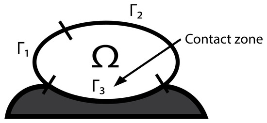
Figure 1. Physical setting.

As contact condition and friction law we firstly use

$$-{\sigma }_{\nu }\left(\mathit{x}\right)=k_0{u}_{\nu }\left(\mathit{x}\right),{\mathbf{\sigma }}_{\tau }\left(\mathit{x}\right)=0(k_{\mathbf{0}}>0).$$

(15)

Secondly we are going to set

$$u_{\nu }\left(\mathit{x}\right)=0,{\mathbf{\sigma }}_{\tau }\left(\mathit{x}\right)=-g\frac{{\mathit{u}}_{\tau }\left(\mathit{x}\right)}{\sqrt{\parallel {\mathit{u}}_{\tau }{\left(\mathit{x}\right)\parallel }^2+{\rho }^2}}(g>0,\rho >0).$$

(16)

As usual, we denoted by $\mathit{u}=\left(u_i\right)$ the displacement field, by $\mathbf{\epsilon }\left(\mathit{u}\right)=\left({\epsilon }_{ij}\left(u\right)\right)$ the infinitesimal strain tensor and by $\mathbf{\sigma }=\left({\sigma }_{ij}\right)$ the Cauchy stress tensor. The normal and the tangential components of the Cauchy vector on the boundary are defined by the formulas ${\sigma }_{\nu }=\left(\mathbf{\sigma }\mathbf{\nu }\right)·\mathbf{\nu },$ ${\mathbf{\sigma }}_{\tau }=\mathbf{\sigma }\mathbf{\nu }-{\sigma }_{\nu }\mathbf{\nu }$ (see, e.g., [13] (p. 89)), while the normal and the tangential components of the displacement vector on the boundary are defined by the formulas $u_{\nu }=\mathit{u}·\mathbf{\nu },$ ${\mathit{u}}_{\tau }=\mathit{u}-u_{\nu }\mathbf{\nu }$ (see, e.g., [13] (p. 86)).

Thus, each of our models consists of the equilibrium Equation (10), the set-valued constitutive law (11) governed by the constitutive function $\omega :{\mathbb{S}}^3\to \mathbb{R}$, the homogeneous displacement condition (12), the traction condition (13), and one of the boundary conditions (15) and (16). In (15), we have a frictionless contact condition involving the Winkler contact law, a law which describes in a simplified manner the interaction between a deformable body and the soil (see [12]). The boundary condition (16) is a frictional bilateral contact condition involving a static version of a regularized Coulomb friction law, see, e.g., [13] (pp. 107–110). For relevant engineering examples in contact mechanics, we refer, for instance, to [26,27,28].

We study successively the problems (10)–(13) (15) and (10)–(13) (16). Let us make the following assumptions:

Assumption A1.

The constitutive function $\omega :{\mathbb{S}}^3\to \mathbb{R}$ is convex and lower semicontinuous. In addition, there exist $\alpha ,\beta$ such that $1>\beta \ge \alpha >0$ and ${\beta \parallel \mathbf{\epsilon }\parallel }_{{\mathbb{S}}^3}^2\ge \omega \left(\mathbf{\epsilon }\right)\ge \alpha {\parallel \mathbf{\epsilon }\parallel }_{{\mathbb{S}}^3}^2$ for all $\mathbf{\epsilon }\in {\mathbb{S}}^3.$

Assumption A2.

The densities of the volume forces and tractions verify

$$f_0\in L^2{(\Omega )}^3 and f_2\in L^2{\left({\Gamma }_2\right)}^3.$$

(17)

Using a similar technique with that used in [7], Theorem 2 allows us to write the following two-field weak formulation for the problem (10)–(13) (15).

Problem 1.

Find $u\in V$ and $\mathbf{\sigma }\in K_{j_1}(u;f,k_0)$ such that

$$\begin{array}{cc}\hfill b(v,\mathbf{\sigma })-b(u,\mathbf{\sigma })+k_0{j}_1(u,v-u)& \ge {(f,v-u)}_V\mathit{for} \mathit{all} v\in V\hfill \end{array}$$

(18)

$$\begin{array}{cc}\hfill b(u,\mathbf{\mu })-b(u,\mathbf{\sigma })& \ge 0\mathit{for} \mathit{all} \mathbf{\mu }\in K_{j_1}(u;f,k_0),\hfill \end{array}$$

(19)

with $b,$ $j_1,$ $f,$ $K_{j_1}(u;f,k_0)$ as follows.

• The map $b(·,·)$ is the bifunctional

  $$b:V\times L_s^2{(\Omega )}^{3\times 3}\to \mathbb{R},b(v,\mathbf{\mu })={\int }_{\Omega }B(\mathbf{\epsilon }\left(v\right)\left(x\right),\mathbf{\mu }\left(x\right))dx,$$

  (20)

  the map B being the bipotential

  $$B:{\mathbb{S}}^3\times {\mathbb{S}}^3\to \mathbb{R},B(\mathbf{\tau },\mathbf{\mu })=\omega \left(\mathbf{\tau }\right)+{\omega }^{*}\left(\mathbf{\mu }\right).$$

  (21)
  Herein, ${\omega }^{*}$ denotes the Fenchel conjugate of $\omega$,

  $${\omega }^{*}:{\mathbb{S}}^3\to (-\infty ,\infty ],{\omega }^{*}\left(\mathbf{\mu }\right)=\underset{\mathbf{\tau }\in {\mathbb{S}}^3}{sup}\{\mathbf{\mu }:\mathbf{\tau }-\omega \left(\mathbf{\tau }\right)\}.$$

  (22)
  We emphasize that, due to Assumption 1, $\omega \left(\mathbf{\tau }(·)\right)\in L^1(\Omega )$ for all $\mathbf{\tau }\in L_s^2{(\Omega )}^{3\times 3}.$ Moreover, it can be proved that its Fenchel conjugate has a similar property: if $\alpha ,\beta$ are the constants in Assumption 1, then

  $${(1-\beta )\parallel \mathbf{\tau }\parallel }_{{\mathbb{S}}^3}^2\le {\omega }^{*}\left(\mathbf{\tau }\right)\le \frac{1}{4\alpha }{\parallel \mathbf{\tau }\parallel }_{{\mathbb{S}}^3}^2\mathrm{for} \mathrm{all} \mathbf{\tau }\in {\mathbb{S}}^3;$$

  (23)

  see, e.g., [5,6]. It follows that ${\omega }^{*}\left(\mathbf{\tau }(·)\right)\in L^1(\Omega )$ for all $\mathbf{\tau }\in L_s^2{(\Omega )}^{3\times 3}.$ Therefore, $B(\mathbf{\epsilon }\left(v\right)(·),\mathbf{\tau }(·))\in L^1(\Omega )$ for all $v\in V,\mathbf{\tau }\in L_s^2{(\Omega )}^{3\times 3}.$
• The bifunctional $j_1(·,·)$ is defined as follows:

  $$j_1:V\times V\to \mathbb{R},j_1(\mathit{u},\mathit{v})={\int }_{{\Gamma }_3}{u}_{\nu }{v}_{\nu }d\Gamma .$$

  (24)
• The element $\mathit{f}\in V$ is defined as follows:

  $${(\mathit{f},\mathit{v})}_V={\int }_{\Omega }{\mathit{f}}_0·\mathit{v}dx+{\int }_{{\Gamma }_2}{\mathit{f}}_2·\mathbf{\gamma }\mathit{v}d\Gamma \mathrm{for} \mathrm{all} \mathit{v}\in V.$$

  (25)
• Given $k_0>0,$ $K_{j_1}(·;\mathit{f},k_0)$ stands for a variable subset of $L_s^2{(\Omega )}^{3\times 3}$ defined as follows: for each $\mathbf{\phi }\in V,$

  $$\begin{array}{cc}\hfill K_{j_1}(\mathbf{\phi };\mathit{f},k_0)=& \{\mathbf{\mu }\in L_s^2{(\Omega )}^{3\times 3}:{(\mathbf{\mu },\mathbf{\epsilon }\left(\mathit{v}\right))}_{L_s^2{(\Omega )}^{3\times 3}}+k_0{j}_1(\mathbf{\phi },\mathit{v})={(\mathit{f},\mathit{v})}_V\hfill \\ \hfill & \mathrm{for} \mathrm{all} \mathit{v}\in V\}.\hfill \end{array}$$

  (26)

Definition 3.

Any solution $(\mathit{u},\mathbf{\sigma })\in V\times K_{j_1}(\mathit{u};\mathit{f},k_0)$ of Problem 1 is called two-field weak solution for the problem (10)–(13) (15).

The problem (10)–(13) (16) has the following two-field weak formulation.

Problem 2.

Find $\mathit{u}\in W$ and $\mathbf{\sigma }\in K_{j_2}(\mathit{u};\mathit{f},g)$ such that

$$\begin{array}{cc}\hfill b(\mathit{v},\mathbf{\sigma })-b(\mathit{u},\mathbf{\sigma })+g{j}_2(\mathit{u},\mathit{v}-\mathit{u})& \ge {(\mathit{f},\mathit{v}-\mathit{u})}_W\mathit{for} \mathit{all} v\in W\hfill \end{array}$$

(27)

$$\begin{array}{cc}\hfill b(\mathit{u},\mathbf{\mu })-b(\mathit{u},\mathbf{\sigma })& \ge 0\mathit{for} \mathit{all} \mathbf{\mu }\in K_{j_2}(\mathit{u};\mathit{f},g),\hfill \end{array}$$

(28)

with $b,$ $j_2,$ $\mathit{f},$ $K_{j_2}(\mathit{u};\mathit{f},g)$ as below.

• The bifunctional $b(·,·)$ is given as follows:

  $$b:W\times L_s^2{(\Omega )}^{3\times 3}\to \mathbb{R},b(\mathit{v},\mathbf{\mu })={\int }_{\Omega }B(\mathbf{\epsilon }\left(\mathit{v}\right)\left(x\right),\mathbf{\mu }\left(x\right))dx$$

  (29)

  with the bipotential B defined in (21).
• The bifunctional $j_2(·,·)$ is defined as follows:

  $$j_2:W\times W\to \mathbb{R},j_2(\mathit{u},\mathit{v})={\int }_{{\Gamma }_3}\frac{{\mathit{u}}_{\tau }}{\sqrt{\parallel {\mathit{u}}_{\tau }{\parallel }^2+{\rho }^2}}·{\mathit{v}}_{\tau }d\Gamma .$$

  (30)
• The element $\mathit{f}\in W$ is defined as follows:

  $${(\mathit{f},\mathit{v})}_W={\int }_{\Omega }{\mathit{f}}_0·\mathit{v}dx+{\int }_{{\Gamma }_2}{\mathit{f}}_2·\mathbf{\gamma }\mathit{v}d\Gamma \mathrm{for} \mathrm{all} \mathit{v}\in W.$$

  (31)
• Given $g>0$, $K_{j_2}(·;\mathit{f},g)$ denotes a variable subset of $L_s^2{(\Omega )}^{3\times 3}$ defined as follows: for each $\mathbf{\phi }\in W,$

  $$\begin{array}{cc}\hfill K_{j_2}(\mathbf{\phi };\mathit{f},g)=& \{\mathbf{\mu }\in L_s^2{(\Omega )}^{3\times 3}:{(\mathbf{\mu },\mathbf{\epsilon }\left(\mathit{v}\right))}_{L_s^2{(\Omega )}^{3\times 3}}+g{j}_2(\mathbf{\phi },\mathit{v})={(\mathit{f},\mathit{v})}_W\hfill \\ \hfill & \mathrm{for} \mathrm{all} \mathit{v}\in W\}.\hfill \end{array}$$

  (32)

Definition 4.

Any solution $(\mathit{u},\mathbf{\sigma })\in W\times K_{j_2}(\mathit{u};\mathit{f},g)$ of Problem 2 is called two-field weak solution for the problem (10)–(13) (16).

4. Abstract Results

Let $(X,{(·,·)}_X,\parallel ·{\parallel }_X)$ and $(Y,{(·,·)}_Y,\parallel ·{\parallel }_Y)$ be two real Hilbert spaces. The first part of this section is devoted to the study of the solvability for the following variational system.

Problem 3.

Find $u\in X$ and $\sigma \in K_j(u;f,\widehat{g})\subset Y$ such that

$$\begin{array}{cc}\hfill J\left(v\right)-J\left(u\right)+\widehat{g}j(u,v-u)& \ge {(f,v-u)}_X\mathit{for} \mathit{all} v\in X\hfill \end{array}$$

(33)

$$\begin{array}{cc}\hfill J^{*}\left(\mu \right)-J^{*}\left(\sigma \right)& \ge 0\mathit{for} \mathit{all} \mu \in K_j(u;f,\widehat{g}).\hfill \end{array}$$

(34)

In order to prove the existence of at least one solution for Problem 3, we shall assume the following hypotheses.

(H1) 

$f\in X,\widehat{g}>0.$

(H2) 

$j:X\times X\to \mathbb{R}$ is a bifunctional such that

$$j(u,v)={(\nabla \psi \left(u\right),v)}_X\mathrm{for} \mathrm{all} v\in X,$$

(35)

where $\psi :X\to {\mathbb{R}}_{+}$ is a convex, lower semicontinuous and Gâteaux differentiable functional, $\nabla \psi \left(u\right)$ denoting the Gâteaux gradient in $u\in X.$

(H3) 

$J:X\to \mathbb{R}$ is a convex and lower semicontinuous map. In addition, there exists ${\alpha }_1>0$ such that $J\left(v\right)\ge {\alpha }_1{\parallel v\parallel }_X^2$ for all $v\in X$.

(H4) 

$J^{*}:Y\to \mathbb{R}$ is a convex and lower semicontinuous map. In addition, there exists ${\alpha }_2>0$ such that $J^{*}\left(\mu \right)\ge {\alpha }_2{\parallel \mu \parallel }_Y^2$ for all $\mu \in Y$.

(H5) 

For each $\phi \in X,$ $K_j(\phi ;f,\widehat{g})$ is a nonempty closed convex subset of Y.

The first abstract result is given by the following theorem.

Theorem 4.

If (H1)–(H5) hold true, then Problem 3 admits at least one solution. If, in addition, J and $J^{*}$ are strictly convex, then Problem 3 admits a unique solution.

Proof. 

We claim that Problem 3 is equivalent to the following problem:

$\left(\mathcal{P}\right):$ find $u\in X$ and $\sigma \in K_j(u;f,\widehat{g})$ such that

$$\begin{array}{cc}\hfill J\left(v\right)-J\left(u\right)+\widehat{g}\psi \left(v\right)-\widehat{g}\psi \left(u\right)& \ge {(f,v-u)}_X\mathrm{for} \mathrm{all} v\in X\hfill \end{array}$$

(36)

$$\begin{array}{cc}\hfill J^{*}\left(\mu \right)-J^{*}\left(\sigma \right)& \ge 0\mathrm{for} \mathrm{all} \mu \in K_j(u;f,\widehat{g}).\hfill \end{array}$$

(37)

Indeed, according to Theorem 1, due to the convexity and the Gâteaux differentiability of the functional $\psi$ considered in (H2), we have

$$\psi \left(v\right)-\psi \left(u\right)\ge {(\nabla \psi \left(u\right),v-u)}_X.$$

(38)

Note that using (35) the above relation yields

$$\psi \left(v\right)-\psi \left(u\right)\ge j(u,v-u).$$

(39)

As a result, if $(u,\sigma )$ is a solution of Problem 3, then $(u,\sigma )$ verifies $\left(\mathcal{P}\right)$.

Conversely, let $(u,\sigma )\in X\times K_j(u;f,\widehat{g})$ be a solution of $\left(\mathcal{P}\right)$.

Setting in (36) $v=u+t(w-u)$ with $w\in X$ arbitrarily fixed and $t\ne 0$ a real number, then for all $t>0$, we can write

$$\frac{J(u+t(w-u\left)\right)-J\left(u\right)}{t}+\frac{\widehat{g}\psi (u+t(w-u))-\widehat{g}\psi \left(u\right)}{t}\ge \frac{{(f,t(w-u))}_X}{t}.$$

(40)

We now use the convexity of J from (H3) to obtain

$$J\left(w\right)-J\left(u\right)+\frac{\widehat{g}\psi (u+t(w-u))-\widehat{g}\psi \left(u\right)}{t}\ge {(f,w-u)}_X,$$

(41)

for all $t\in (0,1).$ Passing to the limit when $t\searrow 0,$ as $\psi$ is Gâteaux differentiable, we obtain

$$J\left(w\right)-J\left(u\right)+\widehat{g}{(\nabla \psi \left(u\right),w-u)}_X\ge {(f,w-u)}_X\mathrm{for} \mathrm{all} w\in X.$$

(42)

Therefore, if $(u,\sigma )\in X\times K_j(u;f,\widehat{g})$ is a solution of $\left(\mathcal{P}\right)$, then $(u,\sigma )$ verifies Problem 3.

Let us define now the functional

$${\tilde{J}}_{f,\widehat{g}}:X\to \mathbb{R},{\tilde{J}}_{f,\widehat{g}}\left(v\right)=J\left(v\right)+\widehat{g}\psi \left(v\right)-{(f,v)}_X.$$

(43)

Note that $\left(\mathcal{P}\right)$ can be written as follows: find $u\in X$ and $\sigma \in K_j(u;f,\widehat{g})$ such that

$$\begin{array}{cc}\hfill {\tilde{J}}_{f,\widehat{g}}\left(v\right)-{\tilde{J}}_{f,\widehat{g}}\left(u\right)& \ge 0\mathrm{for} \mathrm{all} v\in X\hfill \end{array}$$

(44)

$$\begin{array}{cc}\hfill J^{*}\left(\mu \right)-J^{*}\left(\sigma \right)& \ge 0\mathrm{for} \mathrm{all} \mu \in K_j(u;f,\widehat{g}).\hfill \end{array}$$

(45)

It is easy to observe that ${\tilde{J}}_{f,\widehat{g}}$ is convex, lower semicontinuous and coercive, due to the properties of J and $\psi$ from (H2) and (H3). Therefore, using Theorem 3, we deduce that ${\tilde{J}}_{f,\widehat{g}}$ has at least one minimum on X. Let $u^{*}\in X$ be such an element. Consider now the subset $K_j(u^{*};f,\widehat{g}).$ Keeping in mind (H5) with $\phi =u^{*}$, we note that $K_j(u^{*};f,\widehat{g})$ is a nonempty closed convex set. Since $J^{*}$ fulfills (H4), we apply again Theorem 3 to obtain that $J^{*}$ has at least one minimum ${\sigma }^{*}\in K_j(u^{*};f,\widehat{g})$ on $K_j(u^{*};f,\widehat{g})$. We conclude that $(u^{*},{\sigma }^{*})\in X\times K_j(u^{*};f,\widehat{g})$ is a solution of Problem 3. In order to study the uniqueness, we admit in addition that the functionals J and $J^{*}$ are strictly convex. Then, ${\tilde{J}}_{f,\widehat{g}}$ has a unique minimum u on X, and $J^{*}$ has a unique minimum $\sigma$ on $K_j(u;f,\widehat{g}).$ Therefore, the pair $(u,\sigma )$ is the unique solution of Problem 3. □

We are now interested in finding some properties of the solution. Precisely, we are interested to study the dependence of the solution $(u,\sigma )$ on the data f and $\widehat{g}$. For the next result, we need additional hypotheses.

(H6) 

J and $\psi$ vanish in $0_X$;

(H7) 

There exists ${\beta }_2>0$ such that $J^{*}\left(\mu \right)\le {\beta }_2{\parallel \mu \parallel }_Y^2$ for all $\mu \in Y$;

(H8) 

There exists $C>0$ such that $|j(u,v)|\le {C\parallel u\parallel }_X{\parallel v\parallel }_X$ for all $u,v\in X$;

(H9) 

There exists a linear and continuous operator $T:X\to Y$ such that, for each $u\in X,$ $T(f-\widehat{g}\nabla \psi \left(u\right))\in K_j(u;f,\widehat{g}).$

The next proposition delivers useful information that is exploited for the later results.

Proposition 1.

Consider (H1)–(H9). Let $(u,\sigma )$ be a solution of Problem 3. Then,

$$\begin{array}{ccc}& {\parallel u\parallel }_X& \le \frac{1}{{\alpha }_1}{\parallel f\parallel }_X;\hfill \end{array}$$

(46)

$$\begin{array}{cc}\hfill {\parallel \nabla \psi \left(u\right)\parallel }_X& \le \frac{C}{{\alpha }_1}{\parallel f\parallel }_X;\hfill \end{array}$$

(47)

$$\begin{array}{cc}\hfill {\parallel \sigma \parallel }_Y& \le \frac{{\parallel T\parallel }_{\mathcal{L}(X,Y)}}{{\alpha }_1}\sqrt{\frac{2{\beta }_{2}max\{1,{\widehat{g}}^2\}({\alpha }_1^2+C^2)}{{\alpha }_2}}{\parallel f\parallel }_X.\hfill \end{array}$$

(48)

Proof. 

To prove (46), we take $v=0_X$ in (36), and due to (H6), we obtain

$$J\left(u\right)+\widehat{g}\psi \left(u\right)\le {(f,u)}_X.$$

(49)

As $\psi \left(u\right)\ge 0$ (see (H2)) and $\widehat{g}>0$ (see (H1)), by using (H3), we obtain

$${\alpha }_1{\parallel u\parallel }_X^2\le {\parallel f\parallel }_X{\parallel u\parallel }_X,$$

(50)

which implies (46).

In order to obtain (47), we firstly write

$${\parallel \nabla \psi \left(u\right)\parallel }_X=\underset{v\in X,v\ne 0_X}{sup}\frac{{(\nabla \psi \left(u\right),v)}_X}{{\parallel v\parallel }_X}.$$

(51)

Let $v\in X,$ $v\ne 0_X.$ Then, by (H8), we have

$$\frac{{(\nabla \psi \left(u\right),v)}_X}{{\parallel v\parallel }_X}\le \frac{|j(u,v)|}{{\parallel v\parallel }_X}\le C{\parallel u\parallel }_X.$$

(52)

Hence, by using (46), we immediately obtain (47).

Finally, let us prove (48). Since $(u,\sigma )$ is a solution of Problem 3, then

$$J^{*}\left(\mu \right)-J^{*}\left(\sigma \right)\ge 0\mathrm{for} \mathrm{all} \mu \in K_j(u;f,\widehat{g}).$$

(53)

The above inequality and the hypotheses (H4) and (H7) lead us to

$${\alpha }_2{\parallel \sigma \parallel }_Y^2\le {\beta }_2{\parallel \mu \parallel }_Y^2\mathrm{for} \mathrm{all} \mu \in K_j(u;f,\widehat{g}).$$

(54)

Since (H9) holds, let us take $\mu =T(f-\widehat{g}\nabla \psi \left(u\right))$ in (54). From the linearity and continuity of T, we know that $\parallel T(f-\widehat{g}\nabla \psi \left(u\right)){\parallel }_Y\le {\parallel T\parallel }_{\mathcal{L}(X,Y)}{\parallel f-\widehat{g}\nabla \psi \left(u\right)\parallel }_X.$ Hence, we obtain

$${\alpha }_2{\parallel \sigma \parallel }_Y^2\le {\beta }_2{\parallel T\parallel }_{\mathcal{L}(X,Y)}^2{\parallel f-\widehat{g}\nabla \psi \left(u\right)\parallel }_X^2,$$

(55)

which leads to

$${\parallel \sigma \parallel }_Y^2\le \frac{2{\beta }_2{\parallel T\parallel }_{\mathcal{L}(X,Y)}^{2}max\{1,{\widehat{g}}^2\}}{{\alpha }_2}\left({\parallel f\parallel }_X^2+{\parallel \nabla \psi \left(u\right)\parallel }_X^2\right).$$

(56)

Using (47), we can write

$${\parallel \sigma \parallel }_Y^2\le \frac{2{\beta }_2{\parallel T\parallel }_{\mathcal{L}(X,Y)}^{2}max\{1,{\widehat{g}}^2\}\left(1+\frac{C^2}{{\alpha }_1^2}\right)}{{\alpha }_2}{\parallel f\parallel }_X^2,$$

(57)

and from this, we easily obtain (48). □

For the next result, we need new hypotheses.

(H10) 

$J^{*}$ is upper semicontinuous.

(H11) 

If ${\left({\phi }_n\right)}_n,{\left(f_n\right)}_n\subset X$, and ${\left({\widehat{g}}_n\right)}_n\subset (0,\infty )$ are three sequences and $\phi ,f\in X,\widehat{g}\in (0,\infty )$ are three elements such that

$${\phi }_n\rightharpoonup \phi \mathrm{in} X,f_n\to f \mathrm{in} X \mathrm{and} {\widehat{g}}_n\to \widehat{g} \mathrm{in} \mathbb{R}$$

(58)

then $K_j({\phi }_n;f_n,{\widehat{g}}_n)\stackrel{\mathrm{M}}{\to }{K}_j(\phi ;f,\widehat{g}).$

We are now in the position to prove our next abstract result, which shows how the solution depends on the data.

Theorem 5.

We admit (H1)–(H11), and in addition, we assume that J and $J^{*}$ are strictly convex. The operator

$$S:X\times \mathbb{R}\to X\times Y,S(f,\widehat{g})=(u,\sigma )$$

(59)

associated with Problem 3 is demicontinuous.

Proof. 

Let ${\left(f_n\right)}_n\subset X$ be a convergent sequence to f, and let ${\left({\widehat{g}}_n\right)}_n\subset (0,\infty )$ be a convergent sequence to $\widehat{g}>0.$ Let n be a positive integer, and let $(u_n,{\sigma }_n)$ be the unique solution of Problem 3 corresponding to $(f_n,{\widehat{g}}_n).$ We denote by $(u,\sigma )$ the unique solution of Problem 3 corresponding to $(f,\widehat{g})$.

Since ${\left(f_n\right)}_n\subset X$ is a convergent sequence, then there exists $M>0$ such that

$$\parallel f_n{\parallel }_X\le M\mathrm{for} \mathrm{all} n\in \mathbb{N}.$$

(60)

Keeping in mind Proposition 1, by (60) we obtain

$$\parallel u_n{\parallel }_X\le \frac{M}{{\alpha }_1}\mathrm{for} \mathrm{all} n\in \mathbb{N},$$

(61)

which means that the sequence ${\left(u_n\right)}_n\subset X$ is bounded. Therefore, there exists a subsequence ${\left(u_{n_k}\right)}_{n_k}$ and an element $\tilde{u}\in X$ such that

$$u_{n_k}\rightharpoonup \tilde{u}inX.$$

(62)

On the other hand, keeping in mind Proposition 1, for each $n_k,$

$$\parallel {\sigma }_{n_k}{\parallel }_Y\le \frac{{\parallel T\parallel }_{\mathcal{L}(X,Y)}}{{\alpha }_1}\sqrt{\frac{2{\beta }_{2}max\{1,{\widehat{g}}_{n_k}^2\}({\alpha }_1^2+C^2)}{{\alpha }_2}}{\parallel f_{n_k}\parallel }_X.$$

(63)

As ${\left(f_{n_k}\right)}_{n_k}\subset X$ and ${\left({\widehat{g}}_{n_k}\right)}_{n_k}\subset (0,\infty )$ are bounded sequences, then there exists $\tilde{M}>0$ such that

$$\parallel {\sigma }_{n_k}{\parallel }_Y\le \tilde{M},$$

(64)

which implies that there exists a subsequence ${\left({\sigma }_{n^{\prime }}\right)}_{n^{\prime }}$ of ${\left({\sigma }_{n_k}\right)}_{n_k}$ such that

$${\sigma }_{n^{\prime }}\rightharpoonup \tilde{\sigma }\mathrm{in} Y \mathrm{as} n^{\prime }\to \infty .$$

(65)

As a result, there exist ${\left(u_{n^{\prime }}\right)}_{n^{\prime }}\subset X$ and ${\left({\sigma }_{n^{\prime }}\right)}_{n^{\prime }}\subset Y$ such that

$$(u_{n^{\prime }},{\sigma }_{n^{\prime }})\rightharpoonup (\tilde{u},\tilde{\sigma })\mathrm{in} X\times Y \mathrm{as} n^{\prime }\to \infty ,$$

(66)

$(u_{n^{\prime }},{\sigma }_{n^{\prime }})$ being the unique solution of Problem 3 corresponding to the data $(f_{n^{\prime }},{\widehat{g}}_{n^{\prime }})$ for a fixed $n^{\prime }.$

We know that the following inequality holds:

$$J\left(v\right)-J\left(u_{n^{\prime }}\right)+{\widehat{g}}_{n^{\prime }}\psi \left(v\right)-{\widehat{g}}_{n^{\prime }}\psi \left(u_{n^{\prime }}\right)\ge {(f_{n^{\prime }},v-u_{n^{\prime }})}_X\mathrm{for} \mathrm{all} v\in X.$$

(67)

Taking the limsup as $n^{\prime }\to \infty$ in (67), since J and $\psi$ are convex and lower semicontinuous, we obtain

$$J\left(v\right)-J\left(\tilde{u}\right)+\widehat{g}\psi \left(v\right)-\widehat{g}\psi \left(\tilde{u}\right)\ge {(f,v-\tilde{u})}_X\mathrm{for} \mathrm{all} v\in X.$$

(68)

We also know that the following inequality holds:

$$J^{*}\left({\mu }_{n^{\prime }}\right)-J^{*}\left({\sigma }_{n^{\prime }}\right)\ge 0\mathrm{for} \mathrm{all} {\mu }_{n^{\prime }}\in K_j(u_{n^{\prime }};f_{n^{\prime }},{\widehat{g}}_{n^{\prime }}).$$

(69)

We want to prove that for all $\mu \in K_j(\tilde{u};f,\widehat{g})$, we have

$$J^{*}\left(\mu \right)-J^{*}\left(\tilde{\sigma }\right)\ge 0.$$

(70)

For this purpose, let $\mu \in K_j(\tilde{u};f,\widehat{g})$. Notice that (H10) implies

$$K_j(u_{n^{\prime }};f_{n^{\prime }},{\widehat{g}}_{n^{\prime }})\stackrel{\mathrm{M}}{\to }{K}_j(\tilde{u};f,\widehat{g}).$$

(71)

Therefore, there exists ${\left({\tilde{\mu }}_{n^{\prime }}\right)}_{n^{\prime }}\subset Y$ such that ${\tilde{\mu }}_{n^{\prime }}\in K_j(u_{n^{\prime }};f_{n^{\prime }},{\widehat{g}}_{n^{\prime }})$ for each $n^{\prime }\in \mathbb{N}$ and ${\tilde{\mu }}_{n^{\prime }}\to \mu$ in Y as $n^{\prime }\to \infty .$

Hence, we can write

$$J^{*}\left({\tilde{\mu }}_{n^{\prime }}\right)\ge J^{*}\left({\sigma }_{n^{\prime }}\right),$$

(72)

and passing to the limsup as $n^{\prime }\to \infty$ in the above inequality, using (H9) and the fact that $J^{*}$ is convex and lower semicontinuous, we obtain

$$J^{*}\left(\mu \right)\ge J^{*}\left(\tilde{\sigma }\right).$$

(73)

In addition, as ${\sigma }_{n^{\prime }}\rightharpoonup \tilde{\sigma }$ as $n^{\prime }\to \infty$ and ${\sigma }_{n^{\prime }}\in K_j(u_{n^{\prime }};f_{n^{\prime }},{\widehat{g}}_{n^{\prime }})$ for each $n^{\prime }$, then we have from (71) that $\tilde{\sigma }\in K_j(\tilde{u};f,\widehat{g}).$ Therefore, keeping in mind (68) and (73), we deduce that $(\tilde{u},\tilde{\sigma })$ is a solution of Problem 3 corresponding to f and $\widehat{g}$. Since $(u,\sigma )$ is the unique solution of Problem 3 corresponding to $(f,\widehat{g})$, we deduce that $\tilde{u}=u,$ $\tilde{\sigma }=\sigma$ and

$$\begin{array}{cc}\hfill u_{n^{\prime }}& \rightharpoonup u \mathrm{as} n^{\prime }\to \infty ,\hfill \end{array}$$

(74)

$$\begin{array}{cc}\hfill {\sigma }_{n^{\prime }}& \rightharpoonup \sigma \mathrm{as} n^{\prime }\to \infty .\hfill \end{array}$$

(75)

Thus, the weak limits are independent of the subsequences. Consequently, the entire sequences ${\left(u_n\right)}_n$ and ${\left({\sigma }_n\right)}_n$ are weakly convergent to u and $\sigma ,$ respectively. Then,

$$\begin{array}{c}\hfill (u_n,{\sigma }_n)\rightharpoonup (u,\sigma ).\end{array}$$

(76)

Therefore, $S(f_n,{\widehat{g}}_n)\rightharpoonup S(f,\widehat{g}),$ which concludes that S is demicontinuous. □

5. Well-Posedness

In this section, we use the abstract results from Section 4 in order to study the existence, the uniqueness and the dependence on the data of the weak solutions of the models described in Section 3. At the beginning of this study, our aim is to prove that Problem 1 and Problem 2 admit at least one solution, and also to discuss on the uniqueness.

Before we delve into this analysis, we prove a useful lemma.

Lemma 1.

The subsets $K_{j_1}(·;\mathit{f},k_0)$ and $K_{j_2}(·;\mathit{f},g)$ defined in (26) and (32) satisfy (H5).

Proof. 

Let $\mathbf{\phi }\in V$ be arbitrarily fixed. Since $V\ni \mathit{v}\to j_1(\mathbf{\phi },\mathit{v})$ is a linear and continuous mapping, then there exists $\overline{\mathbf{\phi }}\in V$ such that

$$j_1(\mathbf{\phi },\mathit{v})={(\overline{\mathbf{\phi }},\mathit{v})}_V.$$

(77)

It is easy to observe that $\mathbf{\epsilon }(\mathit{f}-k_0\overline{\mathbf{\phi }})$ is an element of $K_{j_1}(\mathbf{\phi };\mathit{f},k_0)$; therefore, the set is nonempty.

Analogously, let $\mathbf{\phi }\in W$ be arbitrarily fixed. As $W\ni \mathit{v}\to j_2(\mathbf{\phi },\mathit{v})$ is a linear and continuous mapping, then there exists $\tilde{\mathbf{\phi }}\in W$ such that

$$j_2(\mathbf{\phi },\mathit{v})={(\tilde{\mathbf{\phi }},\mathit{v})}_W.$$

(78)

As a result, $\mathbf{\epsilon }(\mathit{f}-g\tilde{\mathbf{\phi }})$ is an element of $K_{j_2}(\mathbf{\phi };\mathit{f},g)$. Hence, the set $K_{j_2}(\mathbf{\phi };\mathit{f},g)$ is nonempty. Moreover, by using standard arguments, we deduce that $K_{j_1}(\mathbf{\phi };\mathit{f},k_0)$ and $K_{j_2}(\mathbf{\phi };\mathit{f},g)$ are closed and convex sets. □

The solvability of Problem 1 can be established with the help of Theorem 4 as the following result shows.

Theorem 6.

Under Assumptions 1 and 2, Problem 1 has at least one solution. If, in addition, ω and ${\omega }^{*}$ are strictly convex, then Problem 1 has a unique solution.

Proof. 

Since the bifunctional $b(·,·)$ given by (20) can be written as

$$b(\mathit{v},\mathbf{\mu })=J\left(\mathit{v}\right)+J^{*}\left(\mathbf{\mu }\right),$$

(79)

where

$$J:V\to \mathbb{R},J\left(\mathit{v}\right)={\int }_{\Omega }\omega \left(\mathbf{\epsilon }\left(\mathit{v}\right)\left(\mathit{x}\right)\right)dx$$

(80)

and

$$J^{*}:L_s^2{(\Omega )}^{3\times 3}\to \mathbb{R},J^{*}\left(\mathbf{\mu }\right)={\int }_{\Omega }{\omega }^{*}\left(\mathbf{\mu }\left(\mathit{x}\right)\right)dx,$$

(81)

then we easily observe that

$$\begin{array}{ccc}\hfill b(\mathit{v},\mathbf{\sigma })-b(\mathit{u},\mathbf{\sigma })& =& J\left(\mathit{v}\right)-J\left(\mathit{u}\right)\hfill \end{array}$$

(82)

$$\begin{array}{ccc}\hfill b(\mathit{u},\mathbf{\mu })-b(\mathit{u},\mathbf{\sigma })& =& J^{*}\left(\mathbf{\mu }\right)-J^{*}\left(\mathbf{\sigma }\right).\hfill \end{array}$$

(83)

In consequence, Problem 1 can be equivalently written as follows: find $\mathit{u}\in V$ and $\mathbf{\sigma }\in K_{j_1}(\mathit{u};\mathit{f},k_0)$ such that

$$\begin{array}{cc}\hfill J\left(\mathit{v}\right)-J\left(\mathit{u}\right)+k_0{j}_1(\mathit{u},\mathit{v}-\mathit{u})& \ge {(\mathit{f},\mathit{v}-\mathit{u})}_V\mathrm{for} \mathrm{all} \mathit{v}\in V\hfill \end{array}$$

(84)

$$\begin{array}{cc}\hfill J^{*}\left(\mathbf{\mu }\right)-J^{*}\left(\mathbf{\sigma }\right)& \ge 0\mathrm{for} \mathrm{all} \mathbf{\mu }\in K_{j_1}(\mathit{u};\mathit{f},k_0).\hfill \end{array}$$

(85)

In the sequel, we will apply Theorem 4 with $X=V,$ $Y=L_s^2{(\Omega )}^{3\times 3},$ $J,$ $J^{*}$ given by (80) and (81), $j=j_1$ given by (24), $\mathit{f}=\mathit{f}$ given by (25) and $\widehat{g}=k_0.$ With this end in view, we have to verify (H1)–(H5).

As $\mathit{f}\in V$ and $k_0>0$, (H1) is fulfilled. To proceed, we introduce the functional

$${\psi }_1:V\to {\mathbb{R}}_{+},{\psi }_1\left(\mathit{v}\right)=\frac{1}{2}{\int }_{{\Gamma }_3}{|v_{\nu }|}^{2}d\Gamma \mathrm{for} \mathrm{all} \mathit{v}\in V.$$

(86)

Obviously, ${\psi }_1$ is convex, lower semicontinuous and Gâteaux differentiable, the Gâteaux gradient in $\mathit{u}\in V$ denoted by $\nabla {\psi }_1\left(\mathit{u}\right)$ verifying

$${(\nabla {\psi }_1\left(\mathit{u}\right),\mathit{v})}_V=j_1(\mathit{u},\mathit{v})\mathrm{for} \mathrm{all} \mathit{v}\in V.$$

(87)

Therefore, (H2) is fulfilled. Next, by considering Assumption 1, we deduce that the functionals J and $J^{*}$ given by (80) and (81) satisfy (H3) and (H4). Finally, Lemma 1 ensures that $K_{j_1}(·;\mathit{f},k_0)$ fulfills (H5). Consequently, we can apply Theorem 4 in order to obtain the existence of at least one solution for Problem 1.

If, in addition, $\omega$ and ${\omega }^{*}$ are strictly convex, then the functionals J and $J^{*}$ are strictly convex. As a result, Theorem 4 ensures also the uniqueness. □

Below, we focus on Problem 2.

Theorem 7.

Under Assumptions 1 and 2, Problem 2 has at least one solution. If, in addition, ω and ${\omega }^{*}$ are strictly convex, then Problem 2 has a unique solution.

Proof. 

We observe that the bifunctional $b(·,·)$ given by (29) can be written as

$$b(\mathit{v},\mathbf{\mu })=J\left(\mathit{v}\right)+J^{*}\left(\mathbf{\mu }\right),$$

(88)

where

$$J:W\to \mathbb{R},J\left(\mathit{v}\right)={\int }_{\Omega }\omega \left(\mathbf{\epsilon }\left(\mathit{v}\right)\left(\mathit{x}\right)\right)dx$$

(89)

and $J^{*}$ is given by (81), and then

$$\begin{array}{ccc}\hfill b(\mathit{v},\mathbf{\sigma })-b(\mathit{u},\mathbf{\sigma })& =& J\left(\mathit{v}\right)-J\left(\mathit{u}\right)\hfill \end{array}$$

(90)

$$\begin{array}{ccc}\hfill b(\mathit{u},\mathbf{\mu })-b(\mathit{u},\mathbf{\sigma })& =& J^{*}\left(\mathbf{\mu }\right)-J^{*}\left(\mathbf{\sigma }\right).\hfill \end{array}$$

(91)

Thus, Problem 2 can be equivalently written as follows: find $\mathit{u}\in W$ and $\mathbf{\sigma }\in K_{j_2}(\mathit{u};\mathit{f},g)$ such that

$$\begin{array}{cc}\hfill J\left(\mathit{v}\right)-J\left(\mathit{u}\right)+g{j}_2(\mathit{u},\mathit{v}-\mathit{u})& \ge {(\mathit{f},\mathit{v}-\mathit{u})}_W\mathrm{for} \mathrm{all} \mathit{v}\in W\hfill \end{array}$$

(92)

$$\begin{array}{cc}\hfill J^{*}\left(\mathbf{\mu }\right)-J^{*}\left(\mathbf{\sigma }\right)& \ge 0\mathrm{for} \mathrm{all} \mathbf{\mu }\in K_{j_2}(\mathit{u};\mathit{f},g).\hfill \end{array}$$

(93)

Therefore, we are going to apply Theorem 4 with $X=W,$ $Y=L_s^2{(\Omega )}^{3\times 3},$ $J,$ $J^{*}$ given by (89) and (81), $j=j_2$ given by (30), $f=\mathit{f}$ given by (31) and $\widehat{g}=g.$ Thus, we have to verify (H1)–(H5).

As $\mathit{f}\in W$ and $g>0,$ (H1) is fulfilled. In order to verify (H2), we define the following functional inspired by [13] (pp. 150–152):

$${\psi }_2:W\to {\mathbb{R}}_{+},{\psi }_2\left(\mathit{v}\right)={\int }_{{\Gamma }_3}(\sqrt{\parallel {\mathit{v}}_{\tau }{\parallel }^2+{\rho }^2}-\rho )d\Gamma \mathrm{for} \mathrm{all} \mathit{v}\in W;$$

(94)

the functional ${\psi }_2$ is convex, lower semicontinuous and Gâteaux differentiable, the Gâteaux gradient in $\mathit{u}\in W$ denoted by $\nabla {\psi }_2\left(\mathit{u}\right)$ verifying

$${(\nabla {\psi }_2\left(\mathit{u}\right),\mathit{v})}_W=j_2(\mathit{u},\mathit{v})\mathrm{for} \mathrm{all} \mathit{v}\in W.$$

(95)

Therefore, (H2) is fulfilled. By considering the functional J defined in (89) and the functional $J^{*}$ defined in (81), then (H3) and (H4) are also fulfilled. Finally, from Lemma 1, we have (H5). The claim follows straightforwardly from Theorem 4. □

Next, we turn our attention to the question of how the weak solutions of the problems (10)–(13) (15) and (10)–(13) (16) depend on the data. With this end in view, we firstly prove the following lemma.

Lemma 2.

The subsets $K_{j_1}(·;f,k_0)$ and $K_{j_2}(·;f,g)$ defined in (26) and (32) satisfy (H11).

Proof. 

We consider the case corresponding to $j_2$ because the case corresponding to $j_1$ is easier. Let ${\left({\mathbf{\phi }}_n\right)}_n,{\left(f_n\right)}_n\subset W$ and ${\left(g_n\right)}_n\subset (0,\infty )$ be three sequences, and let $\mathbf{\phi },f\in W$, $g\in (0,\infty )$ be three elements such that

$$\begin{array}{cc}\hfill {\mathbf{\phi }}_n& \rightharpoonup \mathbf{\phi } \mathrm{in} W,\hfill \end{array}$$

(96)

$$\begin{array}{cc}\hfill {\mathit{f}}_n& \to \mathit{f} \mathrm{in} W,\hfill \end{array}$$

(97)

$$\begin{array}{cc}\hfill g_n& \to g \mathrm{in} \mathbb{R}.\hfill \end{array}$$

(98)

In order to prove that $K_{j_2}({\mathbf{\phi }}_n;{\mathit{f}}_n,g_n)\stackrel{\mathrm{M}}{\to }{K}_{j_2}(\mathbf{\phi };\mathit{f},g)$, we have to check the conditions in Definition 2. To start, we prove that for every sequence ${\left({\mathbf{\mu }}_n\right)}_n$ such that ${\mathbf{\mu }}_n\in K_{j_2}({\mathbf{\phi }}_n;{\mathit{f}}_n,g_n)$ for each $n\in \mathbb{N}$ and ${\mathbf{\mu }}_n\rightharpoonup \mathbf{\mu }$ in $L_s^2{(\Omega )}^{3\times 3}$, we have $\mathbf{\mu }\in K_{j_2}(\mathbf{\phi };\mathit{f},g)$.

Let ${\left({\mathbf{\mu }}_n\right)}_n\subset {\left(K_{j_2}({\mathbf{\phi }}_n;{\mathit{f}}_n,g_n)\right)}_n$ be such that ${\mathbf{\mu }}_n\rightharpoonup \mathbf{\mu }$ in $L_s^2{(\Omega )}^{3\times 3}$ as $n\to \infty$.

It holds

$${({\mathbf{\mu }}_n,\mathbf{\epsilon }\left(\mathit{v}\right))}_{L_s^2{(\Omega )}^{3\times 3}}+g_n{j}_2({\mathbf{\phi }}_n,\mathit{v})={({\mathit{f}}_n,\mathit{v})}_W\mathrm{for} \mathrm{all} \mathit{v}\in W.$$

(99)

Let $\mathit{v}\in W.$ It is worth emphasizing that

$$|j_2({\mathbf{\phi }}_n,\mathit{v})-j_2(\mathbf{\phi },\mathit{v})|\le {\int }_{{\Gamma }_3}\parallel \frac{{\left({\mathbf{\phi }}_n\right)}_{\tau }}{\sqrt{\parallel {\left({\mathbf{\phi }}_n\right)}_{\tau }{\parallel }^2+{\rho }^2}}-\frac{{\mathbf{\phi }}_{\tau }}{\sqrt{\parallel {\mathbf{\phi }}_{\tau }{\parallel }^2+{\rho }^2}}\parallel \parallel {\mathit{v}}_{\tau }\parallel d\Gamma .$$

(100)

We now use the fact that

$$\parallel \frac{{\left({\mathbf{\phi }}_n\right)}_{\tau }\left(x\right)}{\sqrt{\parallel {\left({\mathbf{\phi }}_n\right)}_{\tau }\left(x\right){\parallel }^2+{\rho }^2}}-\frac{{\mathbf{\phi }}_{\tau }\left(x\right)}{\sqrt{\parallel {\mathbf{\phi }}_{\tau }{\left(x\right)\parallel }^2+{\rho }^2}}\parallel \le \frac{2}{\rho }\parallel {\left({\mathbf{\phi }}_n\right)}_{\tau }\left(x\right)-{\mathbf{\phi }}_{\tau }\left(x\right)\parallel \mathrm{a.e.} \mathrm{on} {\Gamma }_3$$

(101)

(for a justification of the above inequality, see [13] (pp. 153–154)).

Hence,

$$|j_2({\mathbf{\phi }}_n,\mathit{v})-j_2(\mathbf{\phi },\mathit{v})|\le \frac{2}{\rho }\parallel \mathbf{\gamma }{\mathbf{\phi }}_n{-\mathbf{\gamma }\mathbf{\phi }\parallel }_{L^2{(\Gamma )}^3}{\parallel \mathbf{\gamma }\mathit{v}\parallel }_{L^2{(\Gamma )}^3}.$$

(102)

Since (96) holds and $\mathbf{\gamma }:H^1{(\Omega )}^3\to L^2{(\Gamma )}^3$ is a linear and continuous map, then $j_2({\mathbf{\phi }}_n,\mathit{v})\to j_2(\mathbf{\phi },\mathit{v})$ as $n\to \infty .$

Therefore, by passing to the limit for $n\to \infty$ in (99), we obtain

$${(\mathbf{\mu },\mathbf{\epsilon }\left(\mathit{v}\right))}_{L_s^2{(\Omega )}^{3\times 3}}+g{j}_2(\mathbf{\phi },\mathit{v})={(\mathit{f},\mathit{v})}_W\mathrm{for} \mathrm{all} \mathit{v}\in W,$$

(103)

which concludes that $\mathbf{\mu }\in K_{j_2}(\mathbf{\phi };\mathit{f},g).$

We prove now that for every $\mathbf{\mu }\in K_{j_2}(\mathbf{\phi };\mathit{f},g)$, there exists a sequence ${\left({\mathbf{\mu }}_n\right)}_n$ such that ${\mathbf{\mu }}_n\in K_{j_2}({\mathbf{\phi }}_n;{\mathit{f}}_n,g_n)$ for each $n\in \mathbb{N}$ and ${\mathbf{\mu }}_n\to \mathbf{\mu }$ in $L_s^2{(\Omega )}^{3\times 3}.$

Let $\mathbf{\mu }\in K_{j_2}(\mathbf{\phi };\mathit{f},g)$ be arbitrarily fixed. Let us construct a sequence ${\left({\mathbf{\mu }}_n\right)}_n$ as follows: for each positive integer $n,$

$${\mathbf{\mu }}_n=\mathbf{\mu }-\mathbf{\epsilon }\left(\mathit{f}\right)+\mathbf{\epsilon }\left({\mathit{f}}_n\right)+g\mathbf{\epsilon }\left(\tilde{\mathbf{\phi }}\right)-g_n\mathbf{\epsilon }\left({\tilde{\mathbf{\phi }}}_n\right),$$

(104)

where $\tilde{\mathbf{\phi }}$ is defined in (78) and ${\tilde{\mathbf{\phi }}}_n\in W$ is also obtained from Riesz’s representation theorem, $j_2({\mathbf{\phi }}_n,\mathit{v})={({\tilde{\mathbf{\phi }}}_n,\mathit{v})}_W.$

We claim that ${\mathbf{\mu }}_n\in K_{j_2}({\mathbf{\phi }}_n;{\mathit{f}}_n,g_n)$ for each positive integer $n.$ Indeed, it is easy to observe that

$${({\mathbf{\mu }}_n,\mathbf{\epsilon }\left(\mathit{v}\right))}_{L_s^2{(\Omega )}^{3\times 3}}+g_n{j}_2({\mathbf{\phi }}_n,\mathit{v})={({\mathit{f}}_n,\mathit{v})}_W\mathrm{for} \mathrm{all} \mathit{v}\in W.$$

(105)

On the other hand, by (102), we have

$$\begin{array}{cc}& \parallel {\tilde{\mathbf{\phi }}}_n-\tilde{\mathbf{\phi }}{\parallel }_W=\underset{\mathit{v}\in W,\mathit{v}\ne 0_W}{sup}\frac{{({\tilde{\mathbf{\phi }}}_n-\tilde{\mathbf{\phi }},\mathit{v})}_W}{{\parallel \mathit{v}\parallel }_W}=\underset{\mathit{v}\in W,\mathit{v}\ne 0_W}{sup}\frac{j_2({\mathbf{\phi }}_n,\mathit{v})-j_2(\mathbf{\phi },\mathit{v})}{{\parallel \mathit{v}\parallel }_W}\hfill \\ \hfill & \le \underset{\mathit{v}\in W,\mathit{v}\ne 0_W}{sup}\frac{\frac{2}{\rho }\parallel \mathbf{\gamma }{\mathbf{\phi }}_n{-\mathbf{\gamma }\mathbf{\phi }\parallel }_{L^2{(\Gamma )}^3}{\parallel \mathbf{\gamma }\mathit{v}\parallel }_{L^2{(\Gamma )}^3}}{{\parallel \mathit{v}\parallel }_W}\le \frac{2c_{tr}}{\rho c_K}{\parallel \mathbf{\gamma }{\mathbf{\phi }}_n-\mathbf{\gamma }\mathbf{\phi }\parallel }_{L^2{(\Gamma )}^3}.\hfill \end{array}$$

(106)

Here and everywhere below in this paper, $c_{tr}>0$ and $c_K>0$ stand for the constants appearing in (4) and (6). Using (96) and the fact that $\mathbf{\gamma }:H^1{(\Omega )}^3\to L^2{(\Gamma )}^3$ is a linear and continuous map, we can see that $\parallel \mathbf{\gamma }{\mathbf{\phi }}_n{-\mathbf{\gamma }\mathbf{\phi }\parallel }_{L^2{(\Gamma )}^3}\to 0$ and therefore, ${\tilde{\mathbf{\phi }}}_n\to \tilde{\mathbf{\phi }}$ in W as $n\to \infty .$ As $\mathbf{\epsilon }$ is a linear and continuous operator, see (5), then $\mathbf{\epsilon }\left({\tilde{\mathbf{\phi }}}_n\right)\to \mathbf{\epsilon }\left(\tilde{\mathbf{\phi }}\right)$ as $n\to \infty .$ This convergence, together with (97), (98), and (104), lead to ${\mathbf{\mu }}_n\to \mathbf{\mu }$ in $L_s^2{(\Omega )}^{3\times 3}.$ Analogously, it can be proved that the two conditions in Definition 2 also hold for the subset $K_{j_1}(\mathbf{\phi };f,k_0)$ for each $\mathbf{\phi }\in V.$ □

In the sequel, we consider a new assumption.

Assumption A3.

${\omega }^{*}$ is upper semicontinuous.

Theorem 8.

We admit Assumptions 1–3, and in addition, we assume that ω and ${\omega }^{*}$ are strictly convex. The operator

$$S:V\times \mathbb{R}\to V\times L_s^2{(\Omega )}^{3\times 3},S(\mathit{f},k_0)=(\mathit{u},\mathbf{\sigma })$$

(107)

associated to Problem 1 is demicontinuous.

Proof. 

We are going to apply Theorem 5 with $X=V,$ $Y=L_s^2{(\Omega )}^{3\times 3},$ $J,$ $J^{*}$ given by (80) and (81), $j=j_1$ given by (24), $f=\mathit{f}$ given by (25) and $\widehat{g}=k_0.$ Recall that (H1)–(H5) are fulfilled (see the proof of Theorem 6). By considering Assumption 1, it follows that $J\left({\mathit{0}}_V\right)=0$. Moreover, from (86), it follows that ${\psi }_1\left({\mathit{0}}_V\right)=0$; hence, (H6) is fulfilled too. Assumption 1 also guarantees that (23) holds, and therefore, (H7) is fulfilled. For (H8), note that

$$|j_1{(\mathit{u},\mathit{v})|\le \parallel \mathbf{\gamma }\mathit{u}\parallel }_{L^2{(\Gamma )}^3}{\parallel \mathbf{\gamma }\mathit{v}\parallel }_{L^2{(\Gamma )}^3}\le \frac{c_{tr}^2}{c_K^2}{\parallel \mathit{u}\parallel }_V{\parallel \mathit{v}\parallel }_V\mathrm{for} \mathrm{all} \mathit{u},\mathit{v}\in V.$$

(108)

We can take $C=\frac{c_{tr}^2}{c_K^2}.$ Next, we prove that $\mathbf{\mu }=\mathbf{\epsilon }(\mathit{f}-k_0\nabla {\psi }_1\left(\mathit{u}\right))\in K_{j_1}(\mathit{u};\mathit{f},k_0)$ for each $\mathit{u}\in V.$ We emphasize that, due to (87), we have

$$\begin{array}{cc}& {(\mathbf{\epsilon }(\mathit{f}-k_0\nabla {\psi }_1\left(\mathit{u}\right)),\mathbf{\epsilon }\left(\mathit{v}\right))}_{L_s^2{(\Omega )}^{3\times 3}}+k_0{j}_1(\mathit{u},\mathit{v})\hfill \\ & ={(f-k_0\nabla {\psi }_1\left(\mathit{u}\right),\mathit{v})}_V+k_0{j}_1(\mathit{u},\mathit{v})={(\mathit{f},\mathit{v})}_V-k_0{j}_1(\mathit{u},\mathit{v})+k_0{j}_1(\mathit{u},\mathit{v})\hfill \\ \hfill & ={(\mathit{f},\mathit{v})}_V.\hfill \end{array}$$

(109)

Thus, we can consider the linear and continuous operator $T:V\to L_s^2{(\Omega )}^{3\times 3},$ $T\left(\mathit{v}\right)=\mathbf{\epsilon }\left(\mathit{v}\right);$ hence, (H9) is also fulfilled. Finally, Assumption 3 and Lemma 2 ensure that (H10) and (H11) hold. Therefore, we can apply Theorem 5 to conclude that the operator S associated with Problem 1 is demicontinuous. □

A similar result concerning the solution of Problem 2 can be delivered.

Theorem 9.

We admit Assumptions 1–3, and in addition, we assume that ω and ${\omega }^{*}$ are strictly convex. The operator

$$S:W\times \mathbb{R}\to W\times L_s^2{(\Omega )}^{3\times 3},S(\mathit{f},g)=(\mathit{u},\mathbf{\sigma })$$

(110)

associated with Problem 2 is demicontinuous.

Proof. 

We apply Theorem 5 with $X=W,$ $Y=L_s^2{(\Omega )}^{3\times 3},$ $J,$ $J^{*}$ given by (89), (81), $j=j_2$ given by (30), $f=\mathit{f}$ given by (31) and $\widehat{g}=g.$ As (H1)–(H5) are fulfilled (see the proof of Theorem 7), it remains to check (H6)–(H11). From the definition of ${\psi }_2$ in (94), it is easy to observe that it vanishes in $0_W.$ Actually, we easily observe that (H6) and (H7) hold. Next, we examine if (H8) holds:

$$|j_2(\mathit{u},\mathit{v})|\le \frac{1}{\rho }{\parallel \mathbf{\gamma }\mathit{u}\parallel }_{L^2{(\Gamma )}^3}{\parallel \mathbf{\gamma }\mathit{v}\parallel }_{L^2{(\Gamma )}^3}\le \frac{1}{\rho }\frac{c_{tr}^2}{c_K^2}{\parallel \mathit{u}\parallel }_W{\parallel \mathit{v}\parallel }_W\mathrm{for} \mathrm{all} \mathit{u},\mathit{v}\in W.$$

(111)

We can take $C=\frac{1}{\rho }\frac{c_{tr}^2}{c_K^2}.$

Keeping in mind (95), we observe that

$$\mathbf{\mu }=\mathbf{\epsilon }(\mathit{f}-g\nabla {\psi }_2\left(\mathit{u}\right))\in K_{j_2}(\mathit{u};\mathit{f},g)\mathrm{for} \mathrm{all} \mathit{u}\in W.$$

(112)

Thus, (H9) is fulfilled with $T:W\to L_s^2{(\Omega )}^{3\times 3},$ $T\left(\mathit{v}\right)=\mathbf{\epsilon }\left(\mathit{v}\right)$. Finally, Assumption 3 and Lemma 2 ensure that (H10) and (H11) hold. Therefore, we can apply Theorem 5 to conclude that the operator S associated with Problem 2 is demicontinuous. □

6. Conclusions

The present work is a contribution to the theory of multi-field weak solvability in continuum mechanics by means of an approach based on the theory of bipotentials.

Two contact models were addressed. For each of them, we obtained existence and uniqueness results, and we studied the dependence of the weak solution on the data. Firstly, we made an investigation in an abstract setting covering both models. Then, we applied the abstract results in order to study the well-posedness of each of the two models under consideration.

The weak formulation of the first model consists of the following variational problem: find $\mathit{u}\in V$ and $\mathbf{\sigma }\in K_{j_1}(\mathit{u};\mathit{f},k_0)$ such that

$$\begin{array}{cc}\hfill b(\mathit{v},\mathbf{\sigma })-b(\mathit{u},\mathbf{\sigma })+k_0{j}_1(\mathit{u},\mathit{v}-\mathit{u})& \ge {(\mathit{f},v-\mathit{u})}_V\mathrm{for} \mathrm{all} \mathit{v}\in V\hfill \end{array}$$

(113)

$$\begin{array}{cc}\hfill b(\mathit{u},\mathbf{\mu })-b(\mathit{u},\mathbf{\sigma })& \ge 0\mathrm{for} \mathrm{all} \mathbf{\mu }\in K_{j_1}(\mathit{u};\mathit{f},k_0).\hfill \end{array}$$

(114)

This variational formulation is an alternative to the primal variational formulation: find $\mathit{u}\in V$ such that

$$\begin{array}{cc}\hfill J\left(\mathit{v}\right)-J\left(\mathit{u}\right)+k_0{j}_1(\mathit{u},\mathit{v}-\mathit{u})& \ge {(\mathit{f},\mathit{v}-\mathit{u})}_V\mathrm{for} \mathrm{all} \mathit{v}\in V.\hfill \end{array}$$

(115)

In the classical approach, the stress tensor $\mathbf{\sigma }$ has to verify $\mathbf{\sigma }\left(x\right)\in \partial \omega \left(\mathbf{\epsilon }\right(\mathit{u}\left)\right(x\left)\right)$ a.e. in $\Omega$, where $\mathit{u}\in V$ is the solution of the variational inequality (115).

Similarly, the weak formulation of the second model consists of the following variational problem: find $\mathit{u}\in W$ and $\mathbf{\sigma }\in K_{j_2}(\mathit{u};\mathit{f},g)$ such that

$$\begin{array}{cc}\hfill b(\mathit{v},\mathbf{\sigma })-b(\mathit{u},\mathbf{\sigma })+g{j}_2(\mathit{u},\mathit{v}-\mathit{u})& \ge {(\mathit{f},\mathit{v}-\mathit{u})}_W\mathrm{for} \mathrm{all} \mathit{v}\in W\hfill \end{array}$$

(116)

$$\begin{array}{cc}\hfill b(\mathit{u},\mathbf{\mu })-b(\mathit{u},\mathbf{\sigma })& \ge 0\mathrm{for} \mathrm{all} \mathbf{\mu }\in K_{j_2}(\mathit{u};\mathit{f},g).\hfill \end{array}$$

(117)

This variational system is an alternative to the primal variational formulation: find $\mathit{u}\in W$ such that

$$\begin{array}{cc}\hfill J\left(\mathit{v}\right)-J\left(\mathit{u}\right)+g{j}_2(\mathit{u},\mathit{v}-\mathit{u})& \ge {(\mathit{f},\mathit{v}-\mathit{u})}_W\mathrm{for} \mathrm{all} \mathit{v}\in W.\hfill \end{array}$$

(118)

Thus, in the classical approach, the stress tensor $\mathbf{\sigma }$ has to verify $\mathbf{\sigma }\left(\mathit{x}\right)\in \partial \omega \left(\mathbf{\epsilon }\right(\mathit{u}\left)\right(\mathit{x}\left)\right)$ a.e. in $\Omega$, where $\mathit{u}\in W$ is the solution of the variational inequality (118).

Notice that, due to the separability property of the form b, both variational problems governed by bipotentials can be equivalently expressed in an abstract setting as follows: find $(u,\sigma )\in X\times K_j(u;f,\widehat{g})$ such that

$$\begin{array}{cc}\hfill J\left(v\right)-J\left(u\right)+\widehat{g}\psi \left(v\right)-\widehat{g}\psi \left(u\right)& \ge {(f,v-u)}_X\mathrm{for} \mathrm{all} v\in X\hfill \end{array}$$

(119)

$$\begin{array}{cc}\hfill J^{*}\left(\mu \right)-J^{*}\left(\sigma \right)& \ge 0\mathrm{for} \mathrm{all} \mu \in K_j(u;f,\widehat{g}).\hfill \end{array}$$

(120)

The unique solution $(u,\sigma )$ can be computed by means of a minimization technique as follows: u is the unique minimizer of the functional ${\tilde{J}}_{f,\widehat{g}}(·)=J(·)+\widehat{g}\psi (·)-{(f,·)}_X$ on X and $\sigma$ is the unique minimizer of $J^{*}(·)$ on $K_j(u;f,\widehat{g}).$ At this stage, it would be interesting to propose efficient algorithms in order to approximate the weak solutions. In addition, it would be of high interest to examine if the abstract theory from this paper can be applied in order to study other models.

References

- Schröder, J.; Iglebüscher, M.; Schwarz, A.; Starke, G. A Prange-Hellinger-Reissner type finite element formulation for small strain elasto-plasticity. Comput. Methods Appl. Mech. Eng. 2017, 317, 400–418. [Google Scholar] [CrossRef]
- Hüeber, S.; Wohlmuth, B. An optimal a priori error estimate for nonlinear multibody contact problems. SIAM J. Numer. Anal. 2005, 43, 156–173. [Google Scholar] [CrossRef]
- Hüeber, S.; Matei, A.; Wohlmuth, B. Efficient algorithms for problems with friction. SIAM J. Sci. Comput. 2007, 29, 70–92. [Google Scholar] [CrossRef]
- Matei, A.; Niculescu, C. Weak solutions via bipotentials in mechanics of deformable solids. J. Math. Anal. Appl. 2011, 379, 15–25. [Google Scholar] [CrossRef] [Green Version]
- Matei, A. A variational approach via bipotentials for unilateral contact problems. J. Math. Anal. Appl. 2013, 397, 371–380. [Google Scholar] [CrossRef]
- Matei, A. A variational approach via bipotentials for a class of frictional contact problems. Acta Appl. Math. 2014, 134, 45–59. [Google Scholar] [CrossRef]
- Matei, A.; Osiceanu, M. Two-field variational formulations for a class of nonlinear mechanical models. Math. Mech. Solids 2022. [Google Scholar] [CrossRef]
- Buliga, M.; de Saxcé, G.; Vallée, C. A variational formulation for constitutive laws described by bipotentials. Math. Mech. Solids 2013, 18, 78–90. [Google Scholar] [CrossRef] [Green Version]
- Buliga, M.; de Saxcé, G.; Vallée, C. Bipotentials for Non-monotone Multivalued Operators: Fundamental Results and Applications. Acta Appl. Math. 2010, 110, 955–972. [Google Scholar] [CrossRef] [Green Version]
- Buliga, M.; de Saxcé, G.; Vallée, C. Existence and construction of bipotentials for graphs of multivalued laws. J. Convex Anal. 2008, 15, 87–104. [Google Scholar]
- Buliga, M.; de Saxcé, G.; Vallée, C. Non-maximal cyclically monotone graphs and construction of a bipotential for the Coulomb’s dry friction law. J. Convex Anal. 2010, 17, 81–94. [Google Scholar]
- Panagiotopoulos, P.D. Inequality Problems in Mechanics and Applications. Convex and Nonconvex Energy Functions; Birkhäuser: Basel, Switzerland, 1985; pp. 83–84. [Google Scholar]
- Sofonea, M.; Matei, A. Mathematical Models in Contact Mechanics; Cambridge University Press: New York, NY, USA, 2012; pp. 29, 30, 86, 88, 89, 107–110, 150–154. [Google Scholar]
- Saramito, P. Complex fluids. Modeling and Algorithms; Springer International Publishing: Cham, Switzerland, 2016. [Google Scholar]
- Versaci, M.; Palumbo, A. Magnetorheological Fluids: Qualitative comparison between a mixture model in the Extended Irreversible Thermodynamics framework and an Herschel–Bulkley experimental elastoviscoplastic model. Int. J. Non-Linear Mech. 2020, 118, 103288. [Google Scholar] [CrossRef]
- Yilmaz, N.; Sahiner, A. Generalization of hyperbolic smoothing approach for non-smooth and non-Lipschitz functions. J. Ind. Manag. Optim. 2021. [Google Scholar] [CrossRef]
- Shi, Z.; Wang, H.; Leung, C.S.; So, H.C.; Member EURASIP. Robust MIMO radar target localization based on lagrange programming neural network. Signal Process. 2020, 174, 107574. [Google Scholar] [CrossRef]
- Nečas, J.; Hlaváček, I. Mathematical Theory of Elastic and Elastico-Plastic Bodies: An Introduction; Elsevier Scientific Publishing Company: Amsterdam, The Netherlands, 1981; p. 79. [Google Scholar]
- Migorski, S.; Ochal, A.; Sofonea, M. Nonlinear Inclusions and Hemivariational Inequalities. Models and Analysis of Contact Problems; Springer: New York, NY, USA, 2013; p. 34. [Google Scholar]
- Kurdila, A.J.; Zabarankin, M. Convex Functional Analysis; Birkhäuser Verlag: Basel, Switzerlad, 2005; pp. 180–183. [Google Scholar]
- Niculescu, C.P.; Persson, L.-E. Convex Functions and Their Applications. A Contemporary Approach; Springer: New York, NY, USA, 2006; pp. 45, 116. [Google Scholar]
- Brézis, H. Functional Analysis, Sobolev Spaces and Partial Differential Equations; Springer: New York, NY, USA, 2011; pp. 138–141. [Google Scholar]
- Struwe, M. Variational Methods. Applications to Nonlinear Partial Differential Equations and Hamiltonian Systems; Springer: Heidelberg, Germany, 1996; pp. 1–73. [Google Scholar]
- De Saxcé, G. Une généralisation de l’inégalité de Fenchel et ses applications aux lois constitutives. C. R. Acad. Sci. 1992, 314, 125–129. [Google Scholar]
- Mosco, U. Convergence of Convex Sets and of Solutions of Variational Inequalities. Adv. Math. 1969, 3, 510–585. [Google Scholar] [CrossRef] [Green Version]
- Laursen, T. Computational Contact and Impact Mechanics; Springer: Heidelberg, Germany, 2002. [Google Scholar]
- Wriggers, P. Computational Contact Mechanics; John Wiley & Sons: Hoboken, NJ, USA, 2002. [Google Scholar]
- Wriggers, P.; Laursen, T. Computational Contact Mechanics; Springer: Wien, Austria, 2007. [Google Scholar]
Publisher’s Note: MDPI stays neutral with regard to jurisdictional claims in published maps and institutional affiliations. |
© 2022 by the authors. Licensee MDPI, Basel, Switzerland. This article is an open access article distributed under the terms and conditions of the Creative Commons Attribution (CC BY) license (https://creativecommons.org/licenses/by/4.0/).