Conditions for Existence of Second-Order and Third-Order Filters for Discrete Systems with Additive Noises

Abstract

The problem of constructing functional optimal observers (filters) for stochastic control systems with additive noises in discrete time are studied in this work. Under the assumption that there is no filter of the first order, necessary and sufficient conditions for the existence of filters of the second and third order are obtained in the canonical basis. Analytical expressions of the transfer function matrix from the input noise to the estimation error are presented. A numerical example is given to compare the performance of filters by the quadratic criterion in the steady state.

1. Introduction

The reduced-order filtering problem occupies an important place in the theory of optimal state estimation. Instead of the traditionally used Kalman filter, which forms an estimate of the total system state vector and has an order that coincides with the order of the system, it is proposed to construct its analogue, a functional filter with a reduced dimension. In this case, the computational effort to implement a functional filter is reduced. In addition, the reduced order of the filter simplifies the analysis of the dynamic system.

The problem under study is at the intersection of two classical problems of state estimation theory: the full order filtering problem for stochastic systems and the design functional observer problem for deterministic systems. The first problem relates to the filtration theory and was solved for non-linear case (even for the non-stationary case) in 1959–1960 by Stratonovich [1,2], and for linear case in 1960–1961 by Kalman and Bucy [3,4], for both continuous and discrete time. The solution to the second problem of constructing functional observers for linear stationary fully defined systems was proposed in 1966 by Luenberger [5]. The further development of the theory of functional observers is reflected in detail in the books by O’Reilly [6] and Korovin and Fomichev [7]. In particular, in [7], the conditions of existence and algorithms for the synthesis of functional observers for linear stationary fully deterministic systems are given for various cases, namely scalar and vector output; and scalar and vector functional. Two methods of solving the design functional observer problem are also proposed: the pseudo-input method and the scalar observer method. Both methods allow one to obtain necessary and sufficient conditions for the existence of functional observers of order k ($k<\nu -1,$ where $\nu$ is the observability index of the system), which were first proposed in [8,9].

Much attention has been paid to the construction of the reduced-order filters for linear systems. Minimizing the quadratic error criterion over the interval and using the solution of the two-point boundary value problem, the reduced-order filter is designed in [10,11]. Based on the quasi-diagonal matrix decomposition and the solution of the Riccati and Lyapunov matrix equations, a method is proposed in [12] for determining the parameters of continuous and digital linear filters of reduced order which ensures their asymptotic stability provided that the estimated system is stabilizable and detectable. In [13,14,15], the proof of the uniqueness of the optimal unbiased reduced-order filter and the properties of the reduced-order innovation process in continuous and discrete time are proposed. Developing the results obtained in [13], the necessary and sufficient conditions for existence, stability, and convergence of the designed filter are obtained for both continuous and discrete stochastic systems in [14], and for discrete stochastic systems with unknown inputs in [15]. In [16], a method for the synthesis of functional optimal observers in the frequency domain using spectral factorization in continuous and discrete time is proposed, and the transfer function of the filter and the properties of its associated innovation sequence are obtained. In [17], using a model reduction of the original system and solving the Lyapunov equations involved in each iteration of the optimum search algorithm, a simple method for reduced-order ${\mathcal{H}}_2$ filter design is proposed. An approach to design a sliding mode control-based functional observer for discrete-time stochastic systems, existence conditions, and stability analysis of the proposed observer are given in [18]. In [19], a generalization of the classical unbiasedness condition in the joint problem of stabilization and optimal filtering is presented, and an alternative method for constructing reduced-order filters is proposed, based on reduction to a non-linear optimization problem. Conditions for existence of second-order and third-order filters for systems in continuous time with additive noises are proposed in [20]. In [21,22], the frequency-weighted ${\mathcal{H}}_2$-optimal model order reduction problem is investigated, and algorithms are proposed, that constructs a reduced-order model, which nearly satisfies the first-order optimality conditions.

In practice, reduced-order optimal filters are used in signal processing of inertial navigation systems, in health parameter estimation for an aircraft turbofan engine, in induction motor state estimation, in dynamic image analysis, in restoration of progressive and interlaced video, in separation of heart and respiratory sounds, in meteorology and oceanography applications (see [23] and references therein).

This article proposes an approach to constructing reduced-order filters, which differs from the methods in [13,14,15,16] in that the filter order does not necessarily coincide with the dimension of the estimated functional. Unlike the methods in [12,17,21,22], where Lyapunov equations are used to calculate the quality criterion, this article uses the method of integral quadratic performance measures, which makes it possible to determine the dependence on parameters in an explicit form.

The problem formulation is presented in Section 2, where the scalar linear functional of the state vector is estimated from the measured scalar output. Perturbations are white random processes with a priori known probabilistic characteristics, uncorrelated with each other at different times and with the initial state of the system. The root-mean-square error in the steady state is chosen as a criterion of optimality. In Section 3, necessary and sufficient conditions for the existence of filters of the second and third order are obtained using canonical forms. Analytical expressions for the transfer function matrix are given in Section 4. The dependence of the parameters number of second-order and third-order filters on the order of original system is presented. Section 5 contains an illustrative example of comparing second and third order filters by quadratic criterion in steady state. Section 6 summarizes the article.

The mathematical notations used in this text are listed in

Table 1. Mathematical notations.

Notation	Meaning
0	zero; zero vector; zero matrix
∈	belongs to
$\mathbb{R}$	the set of real numbers
${·}^{⊺}$	transposition of a vector or matrix
i	integer
j	$\sqrt{-1}$; integer
$\mathbb{E}[·]$	the mathematical expectation operator
${\delta }_{ij}$	Kronecker delta
$\stackrel{\Delta }{=}$	equal by definition
$det(·)$	determinant of the square matrix
z	z-transform variable
$I_k$	identity matrix of dimension $k\times k$
$\theta$	normalized angular frequency
$\omega$	angular frequency
${·}^{-1}$	inverse of the square matrix
$|·|$	magnitude or absolute value of a complex scalar

.

2. Problem Statement

Consider an n–dimensional linear discrete system with stochastic perturbations and with a scalar output:

$$\begin{array}{cc}\hfill x_{i+1}& =A{x}_i+B{u}_i+w_i,\hfill \\ \hfill y_i& =C{x}_i+v_i,\hfill \end{array}i\ge 0,$$

(1)

where $x_i\in {\mathbb{R}}^n$ is the unknown phase vector, $u_i\in {\mathbb{R}}^m$ is the known input of the system, and $y_i\in \mathbb{R}$ is the measured output of the system; A, B, C are constant matrices of appropriate sizes, $w_i$, $v_i$ are discrete uncorrelated, and zero mean white noise processes of dimensions n and 1, respectively, with given covariance matrices $\mathbb{E}[w_i{w}_j^{⊺}]=Q{\delta }_{ij}$, $\mathbb{E}\left[v_i{v}_j\right]=R{\delta }_{ij}$; the initial state $x_0$ is a random variable uncorrelated with noises $w_i$, $v_i$, and has $\mathbb{E}\left[x_0\right]={\overline{x}}_0$, $\mathbb{E}\left[(x_0-{\overline{x}}_0){(x_0-{\overline{x}}_0)}^{⊺}\right]=P_0$. Here, Q, $P_0$ are positive semidefinite matrices; and $R>0$. These assumptions can be represented as

$$\mathbb{E}\left[\left(\begin{array}{c}{w}_i\\ v_i\\ x_0\end{array}\right)\left(\begin{array}{cccc}{w}_j^{⊺}& v_j& x_0^{⊺}& 1\end{array}\right)\right]=\left[\begin{array}{cccc}Q{\delta }_{ij}& 0& 0& 0\\ 0& R{\delta }_{ij}& 0& 0\\ 0& 0& P_0+{\overline{x}}_0{{\overline{x}}_0}^{⊺}& {\overline{x}}_0\end{array}\right],i\ge 0,j\ge 0.$$

It is also assumed that the matrices Q, R, $P_0$ are known a priori. The first equation in the system (1) can be understood in the sense of the stochastic difference equation [24].

Required based on the observation of the output $y_i$ and the known input $u_i$, define an unbiased estimate ${\tilde{\sigma }}_i$ for scalar functional

$${\sigma }_i=F{x}_i,i\ge 0,$$

(2)

with the known matrix $F\in {\mathbb{R}}^{1\times n}$, providing the minimum of the steady state mean value of the squared observation error $e_i\stackrel{\Delta }{=}{\sigma }_i-{\tilde{\sigma }}_i$:

$$J=\underset{i\to \infty }{lim}\mathbb{E}\left[e_i^2\right]\to min.$$

(3)

3. Filter Design

Let matrix F have the standard decomposition [6,7]

$$F=PT+VC,$$

where $P\in {\mathbb{R}}^{1\times k},$$T\in {\mathbb{R}}^{k\times n},$ and $V\in \mathbb{R}.$ Then, ${\sigma }_i=P{q}_i+V{y}_i-V{v}_i,$ where $q_i=T{x}_i\in {\mathbb{R}}^k$ is an unknown vector to be estimated. To reconstruct it, we use an observer of order k

$$\begin{array}{cccc}\hfill {\tilde{q}}_{i+1}& =N{\tilde{q}}_i+TB{u}_i+M{y}_i,\hfill & \hfill {\tilde{q}}_0& =T{\overline{x}}_0,\hfill \\ \hfill {\tilde{\sigma }}_i& =P{\tilde{q}}_i+V{y}_i,\hfill & \hfill \end{array}i\ge 0,$$

(4)

where ${\tilde{q}}_i\in {\mathbb{R}}^k$ is the phase vector of the observer; $N,$ M are constant matrices of appropriate sizes. In the second equation of the observer, the output $y_i$ of the original system (1) appears, which makes it possible to obtain an advantage in terms of the quadratic criterion over the filter without it.

Without loss of generality, we make the following standard [6] assumptions regarding the original system (1) and the desired filter (4).

Assumption 1.

The pair $\{C,A\}$ is observable and is given in the second canonical form of observability [7]

$$A=\left(\begin{array}{ccccc}0& 0& \dots & 0& -{\alpha }_1\\ 1& 0& \dots & 0& -{\alpha }_2\\ \dots & \dots & \dots & \dots & \dots \\ 0& 0& \dots & 1& -{\alpha }_n\end{array}\right),C=\left(\begin{array}{cccc}0& \dots & 0& 1\end{array}\right),$$

(5)

where ${\alpha }_i$ is the coefficients of the characteristic polynomial of the matrix A, i.e.,

$$\alpha (z)=det(z{I}_n-A)=z^n+{\alpha }_n{z}^{n-1}+\dots +{\alpha }_1.$$

The matrix F in the canonical basis has the form:

$$F=\left(\begin{array}{cccc}{f}_1& f_2& \dots & f_n\end{array}\right).$$

Assumption 2.

The pair $\{P,N\}$ is observable and is given in the first canonical form of observability [7]

$$N=\left(\begin{array}{ccccc}0& 1& 0& \dots & 0\\ 0& 0& 1& \dots & 0\\ \dots & \dots & \dots & \dots & \dots \\ 0& 0& 0& \dots & 1\\ -l_1& -l_2& -l_3& \dots & -l_k\end{array}\right),P=\left(\begin{array}{cccc}1& 0& \dots & 0\end{array}\right),$$

(6)

where $l_i$ is the coefficients of the characteristic polynomial of the matrix N, i.e.,

$$\beta (z)=det(z{I}_k-N)=z^k+l_k{z}^{k-1}+\dots +l_1.$$

Let us investigate the question of when linear filters of the second ($k=2$) and third ($k=3$) order can estimate the functional (2) from the state vector. In addition, it is assumed that there is no first-order ($k=1$) filter giving an unbiased estimate for the functional (2). Discrete-time filters of various orders starting from the first order were considered in [25].

Theorem 1.

For system (1) of order higher than the third $(n>3)$ with stochastic perturbations and filters (4) of the second and third order, giving an unbiased estimate of the functional (2) from the state vector, it is true that:

(1) the necessary and sufficient conditions for the existence of a second-order filter have the form

$$\begin{array}{c}T=\left(\begin{array}{ccccc}{f}_1& f_2& \dots & f_{n-1}& f_n-V\\ f_2& f_3& \dots & f_n-V& t_{2n}\end{array}\right),\\ M=\left(\begin{array}{c}-{\displaystyle \sum _{i=1}^n}{\alpha }_i{f}_i-t_{2n}+{\alpha }_{n}V\\ -{\displaystyle \sum _{i=1}^{n-1}}{\alpha }_i{f}_{i+1}-({\alpha }_n-l_2)t_{2n}+l_1(f_n-V)+{\alpha }_{n-1}V\end{array}\right),\\ V=f_n+l_1{f}_{n-2}+l_2{f}_{n-1},t_{2n}=-l_1{f}_{n-1}-l_2(f_n-V),f_1{f}_3-f_2^2\ne 0,\end{array}$$

$$l_1=\frac{f_{2}a-f_3^2}{f_1{f}_3-f_2^2},l_2=\frac{f_2{f}_3-f_{1}a}{f_1{f}_3-f_2^2},1-l_1>0,1-l_2+l_1>0,1+l_1+l_2>0,$$

(7)

$$a=\left\{\begin{array}{c}{f}_4,\mathrm{if}n>4,\hfill \\ f_4-V,\mathrm{if}n=4;\hfill \end{array}\right.f_i=-l_1{f}_{i-2}-l_2{f}_{i-1},i=5,\dots ,n-1,\mathrm{for}n>5,$$

where the condition $f_1{f}_3-f_2^2\ne 0$ means that the observer (4) of the first order cannot reconstruct the unbiased estimate of the functional (2);

(2) the necessary and sufficient conditions for the existence of a third-order filter have the form

$$\begin{array}{c}T=\left(\begin{array}{cccccc}{f}_1& f_2& \dots & f_{n-2}& f_{n-1}& f_n-V\\ f_2& f_3& \dots & f_{n-1}& f_n-V& t_{2n}\\ f_3& f_4& \dots & f_n-V& t_{2n}& t_{3n}\end{array}\right),\\ M=\left(\begin{array}{c}-{\displaystyle \sum _{i=1}^n}{\alpha }_i{f}_i-t_{2n}+{\alpha }_{n}V\\ -{\displaystyle \sum _{i=1}^{n-1}}{\alpha }_i{f}_{i+1}-{\alpha }_n{t}_{2n}-t_{3n}+{\alpha }_{n-1}V\\ -{\displaystyle \sum _{i=1}^{n-2}}{\alpha }_i{f}_{i+2}-({\alpha }_{n-1}-l_2)t_{2n}-({\alpha }_n-l_3)t_{3n}+l_1(f_n-V)+{\alpha }_{n-2}V\end{array}\right),\\ V=f_n+l_1{f}_{n-3}+l_2{f}_{n-2}+l_3{f}_{n-1},\\ t_{2n}=-l_1{f}_{n-2}-l_2{f}_{n-1}-l_3(f_n-V),t_{3n}=-l_1{f}_{n-1}-l_2(f_n-V)-l_3{t}_{2n},\end{array}$$

$$b\ne \frac{f_3(f_3^2-f_{2}a)+a(f_{1}a-f_2{f}_3)}{f_1{f}_3-f_2^2},$$

(8)

$$\begin{array}{c}{l}_1=\frac{a(a^2-f_{3}b)+b(f_{2}b-f_{3}a)+c(f_3^2-f_{2}a)}{b(f_1{f}_3-f_2^2)-f_3(f_3^2-f_{2}a)-a(f_{1}a-f_2{f}_3)},\\ l_2=\frac{a(f_{2}b-f_{3}a)+b(f_3^2-f_{1}b)+c(f_{1}a-f_2{f}_3)}{b(f_1{f}_3-f_2^2)-f_3(f_3^2-f_{2}a)-a(f_{1}a-f_2{f}_3)},\\ l_3=\frac{a(f_3^2-f_{2}a)+b(f_{1}a-f_2{f}_3)+c(f_2^2-f_1{f}_3)}{b(f_1{f}_3-f_2^2)-f_3(f_3^2-f_{2}a)-a(f_{1}a-f_2{f}_3)},\end{array}$$

$$1-l_1^2>0,l_1^2-1<l_1{l}_3-l_2,1+l_3+l_2+l_1>0,-1+l_3-l_2+l_1<0,$$

(9)

$$a=\left\{\begin{array}{c}{f}_4,\mathrm{if}n>4,\hfill \\ f_4-V,\mathrm{if}n=4;\hfill \end{array}\right.b=\left\{\begin{array}{c}{f}_5,\mathrm{if}n>5,\hfill \\ f_5-V,\mathrm{if}n=5,\hfill \\ t_{24},\mathrm{if}n=4;\hfill \end{array}\right.c=\left\{\begin{array}{c}{f}_6,\mathrm{if}n>6,\hfill \\ f_6-V,\mathrm{if}n=6,\hfill \\ t_{25},\mathrm{if}n=5,\hfill \\ t_{34},\mathrm{if}n=4;\hfill \end{array}\right.$$

$$f_i=-l_1{f}_{i-3}-l_2{f}_{i-2}-l_3{f}_{i-1},i=7,\dots ,n-1,\mathrm{for}n>7,$$

where the condition (8) for the case $n>5$ means that the observer (4) of the second order cannot reconstruct the unbiased estimate of the functional (2).

Proof. 

Using the stochastic difference equations of the original system (1) and the observer (4), it is not difficult to obtain that the estimation error $e_i^q\stackrel{\Delta }{=}{q}_i-{\tilde{q}}_i$ is described by the equation

$$\begin{array}{c}{e}_{i+1}^q=q_{i+1}-{\tilde{q}}_{i+1}=T{x}_{i+1}-N{\tilde{q}}_i-TB{u}_i-M{y}_i\hfill \\ \hspace{1em}\hspace{1em}\hspace{1em}\hspace{1em}\hspace{1em}\hspace{1em}\hspace{1em}=TA{x}_i-N(q_i-e_i^q)-MC{x}_i+T{w}_i-M{v}_i\\ \hfill \hspace{1em}\hspace{1em}\hspace{1em}\hspace{1em}\hspace{1em}\hspace{1em}\hspace{1em}\hspace{1em}\hspace{1em}\hspace{1em}\hspace{1em}\hspace{1em}=N{e}_i^q+(TA-MC-NT)x_i+T{w}_i-M{v}_i.\end{array}$$

(10)

The equation for the error $e_i={\sigma }_i-{\tilde{\sigma }}_i$ has the form

$$e_i={\sigma }_i-{\tilde{\sigma }}_i=F{x}_i-P{\tilde{q}}_i-V{y}_i=PT{x}_i+VC{x}_i-P{\tilde{q}}_i-VC{x}_i-V{v}_i=P{e}_i^q-V{v}_i.$$

(11)

Based on the known results [6], we can conclude that the estimates ${\tilde{q}}_i$ and ${\tilde{\sigma }}_i$ are unbiased for $q_i$ and ${\sigma }_i$, respectively, if and only if the following conditions are satisfied:

$$F=PT+VC,TA-MC-NT=0,N\mathrm{is}\mathrm{a}\mathrm{Schur}\mathrm{matrix}.$$

(12)

Moreover, if the matrix N is a Schur matrix, then [26] the observation error $e_i^q$ in the steady state is a stationary in the wide sense random process, in which the mathematical expectation is constant, and the correlation function depends on one variable.

Both statements of the theorem are obtained in a similar way from the conditions (12), Assumption 1 about the canonical representations of the original system (5) and Assumption 2 about the canonical representations of the desired filter (6). □

Remark 1.

Inequalities in Formulas (7) and (9) are discrete stability constraints for the filter (4) obtained using the simplified stability criterion [27] for linear discrete systems.

Remark 2.

If the condition (8) is violated, then there is a set of the degenerate third-order observers whose coefficients of the characteristic polynomial according to Vieta’s formulas have the form

$$l_1=z_1{z}_2(C_1+z_1+z_2),l_2=z_1{z}_2-(z_1+z_2)(C_1+z_1+z_2),l_3=C_1$$

and are located at the intersection of the domain of discrete stability of the matrix N and the solution set for the system of equations

$$z_1^3+l_3{z}_1^2+l_2{z}_1+l_1=0,z_2^3+l_3{z}_2^2+l_2{z}_2+l_1=0,$$

(13)

where $z_1,z_2$ are the roots of the characteristic polynomial $z^2+l_{2}z+l_1$ with coefficients $l_1,l_2$ satisfying (7); and they are determined by the quadratic formula

$$z_{1,2}=\frac{f_{1}a-f_2{f}_3\pm \sqrt{{(f_2{f}_3-f_{1}a)}^2-4(f_{2}a-f_3^2)(f_1{f}_3-f_2^2)}}{2(f_1{f}_3-f_2^2)}.$$

$C_1$ is a free unknown, which is chosen so that the stability conditions (9) are satisfied:

$$-1-z_1-z_2<C_1<1-z_1-z_2,$$

and the variable a is determined according to the second statement of Theorem 1.

4. Transfer Function Matrix of the Estimation Error System

This section discusses a method for calculating the optimality criterion (3) by interpreting [28] the steady state root-mean-square error as ${\mathcal{H}}_2$ norm of the weighted transfer matrix of the estimation error system (10) and (11)

$$J=\underset{i\to \infty }{lim}\mathbb{E}\left[e_i^2\right]=\frac{1}{2\pi }\underset{-\pi }{\overset{\pi }{\int }}{W}_{e\overline{u}}(e^{j\theta })\left(\begin{array}{cc}Q& 0\\ 0& R\end{array}\right)W_{e\overline{u}}^{⊺}(e^{-j\theta })d\theta ,$$

where the transfer function matrix $W_{e\overline{u}}(z)$ from the vector noise ${\overline{u}}_i\stackrel{\Delta }{=}{\left(\begin{array}{cc}{w}_i^{⊺}& v_i\end{array}\right)}^{⊺}$ to the estimation error $e_i$ must be stable and can be found using the following theorem.

Theorem 2.

If the conditions of Theorem 1 are satisfied, then the transfer function matrix $W_{e\overline{u}}(z)$ of the estimation error system has the form

$$W_{e\overline{u}}(z)=\frac{1}{\beta (z)}\left(\begin{array}{cccc}{W}_{ew}^1(z)& \dots & W_{ew}^n(z)& W_{ev}(z)\end{array}\right),$$

(1) in which, for the case of a second-order filter:

$$\begin{array}{c}{W}_{ew}^i(z)=f_i(z+l_2)+f_{i+1},i=1,\dots ,n-2,\\ W_{ew}^{n-1}(z)=f_{n-1}(z+l_2)+f_n-V,W_{ew}^n(z)=(f_n-V)(z+l_2)+t_{2n},\\ W_{ev}(z)=-V\beta (z)+(\sum _{i=1}^n{\alpha }_i{f}_i+t_{2n}-{\alpha }_{n}V)(z+l_2)\\ +\sum _{i=1}^{n-1}{\alpha }_i{f}_{i+1}+({\alpha }_n-l_2)t_{2n}-l_1(f_n-V)-{\alpha }_{n-1}V,\\ \beta (z)=z^2+l_{2}z+l_1;\end{array}$$

(2) in which, for the case of a third-order filter:

$$\begin{array}{c}{W}_{ew}^i(z)=f_i(z^2+l_{3}z+l_2)+f_{i+1}(z+l_3)+f_{i+2},i=1,\dots ,n-3,\\ W_{ew}^{n-2}(z)=f_{n-2}(z^2+l_{3}z+l_2)+f_{n-1}(z+l_3)+f_n-V,\\ W_{ew}^{n-1}(z)=f_{n-1}(z^2+l_{3}z+l_2)+(f_n-V)(z+l_3)+t_{2n},\\ W_{ew}^n(z)=(f_n-V)(z^2+l_{3}z+l_2)+t_{2n}(z+l_3)+t_{3n},\\ W_{ev}(z)=-V\beta (z)+(\sum _{i=1}^n{\alpha }_i{f}_i+t_{2n}-{\alpha }_{n}V)(z^2+l_{3}z+l_2)\\ +(\sum _{i=1}^{n-1}{\alpha }_i{f}_{i+1}+{\alpha }_n{t}_{2n}+t_{3n}-{\alpha }_{n-1}V)(z+l_3)\\ +\sum _{i=1}^{n-2}{\alpha }_i{f}_{i+2}+({\alpha }_{n-1}-l_2)t_{2n}+({\alpha }_n-l_3)t_{3n}-l_1(f_n-V)-{\alpha }_{n-2}V,\\ \beta (z)=z^3+l_3{z}^2+l_{2}z+l_1.\end{array}$$

Proof. 

The estimation error system (10) and (11) can be written as follows:

$$\begin{array}{c}{e}_{i+1}^q=N{e}_i^q+\overline{B}{\overline{u}}_i,e_i=P{e}_i^q+\overline{D}{\overline{u}}_i,i\ge 0,\\ \overline{B}=(T\hspace{1em}-M),\overline{D}=(0\hspace{1em}-V).\end{array}$$

For this system, the transfer function matrix from the input ${\overline{u}}_i$ to the output $e_i$ is equal to

$$W_{e\overline{u}}(z)=P{(z{I}_k-N)}^{-1}\overline{B}+\overline{D}.$$

(14)

Using Formula (14), the necessary and sufficient existence conditions of a filter of the appropriate order from Theorem 1, and Assumption 2 on the canonical representation of the filter, we obtain both statements of Theorem 2. Moreover, the pair $\{P,N\}$ is observable by Assumption 2, and the pair $\{N,\overline{B}\}$ is controllable by the condition $f_1{f}_3-f_2^2\ne 0$ for the second-order filter and by the condition (8) for the third-order filter. Consequently, using the properties [29,30] of the concept of controllability and observability, we obtain that the specified transfer function matrix is irreducible. □

Remark 3.

Depending on the order n of the original system (1) and the order k of the desired filter (4), the transfer function matrix $W_{e\overline{u}}(z)$ has unknown parameters indicated in

Table 2. Transfer function matrix parameters.

The Order of the Original System	The Order of the Desired Filter
	k = 2	k = 3
$n=4$	V	$V,$$t_{24},$$t_{34}$
$n=5$	no parameters	$V,$$t_{25}$
$n=6$		V
$n>6$		no parameters

.

Remark 4.

If the condition (8) of Theorem 1 is violated for a third-order filter, then the transfer matrix of the error system can be calculated according to the first statement of Theorem 2.

There are various ways to find the optimality criterion without calculating the poles of the transfer function. Firstly, calculation J can be reduced to the calculation of integrals

$$\frac{1}{2\pi }\underset{-\pi }{\overset{\pi }{\int }}{\left|\frac{b_0{e}^{j\theta k}+b_1{e}^{j\theta (k-1)}+\dots +b_k}{a_0{e}^{j\theta k}+a_1{e}^{j\theta (k-1)}+\dots +a_k}\right|}^{2}d\theta ,$$

(15)

where the coefficients $a_i,$$b_i$ depend on unknown parameters of the filter (4) according to Theorem 2 and Remark 3. There are special formulas and tables [31,32,33,34,35] for calculating integrals (15).

Secondly, by bilinear transformation [36], calculation J can be reduced to the calculation of integrals

$$\frac{1}{2\pi }\underset{-\infty }{\overset{\infty }{\int }}{\left|\frac{{\tilde{b}}_0{(j\omega )}^k+{\tilde{b}}_1{(j\omega )}^{k-1}+\dots +{\tilde{b}}_k}{{\tilde{a}}_0{(j\omega )}^{k+1}+{\tilde{a}}_1{(j\omega )}^k+\dots +{\tilde{a}}_{k+1}}\right|}^{2}d\omega .$$

(16)

There are also special formulas and tables [35,37,38,39] for calculating integrals (16).

Thirdly, a discrete Lyapunov matrix equation can be used [40] to calculate $J.$

5. Numerical Example

This section presents a numerical example of comparing second and third order filters in terms of the asymptotic quadratic mean observation error.

We consider the system (1) and (2) of the fourth order, in which the matrices $A,$ C are given in the canonical form (5) with ${\alpha }_1=1/16,$ ${\alpha }_2=1/2,$ ${\alpha }_3=3/2,$ ${\alpha }_4=2;$ the matrix B is zero matrix; the elements of the matrix F are equal to $f_1=1,$ $f_2=1/2,$ $f_3=1/3,$ $f_4=1/4;$ the probabilistic characteristics are $Q=P_0=I_4,$ $R=1,$ ${\overline{x}}_0={\left[\begin{array}{cccc}1& 0& 0& 0\end{array}\right]}^{⊺}.$

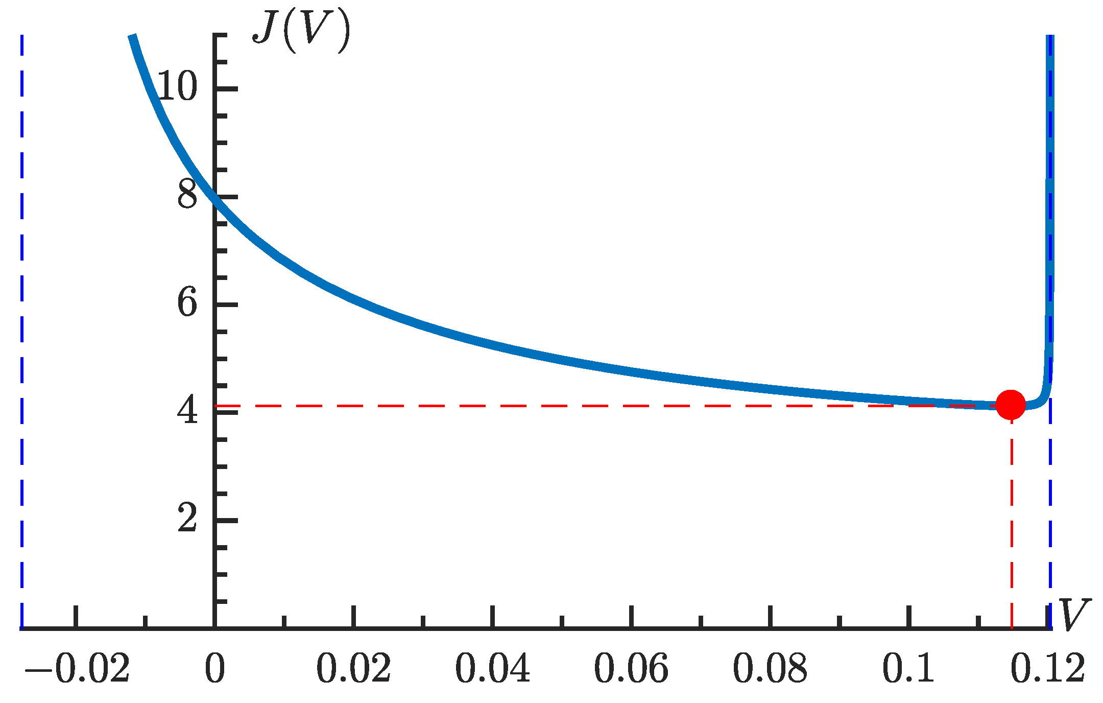
There is no first-order filter reconstructing the unbiased estimate of the scalar functional (2). To find the unknown parameter (V) of the second-order filter (4), we solve the problem of minimizing the optimality criterion (3), which, according to Section 4, is

$$J(V)=\frac{492,687,360V^4+143,928,576V^3+55,244,160V^2-6,303,956V-396,985}{768(36V+1)(36V+5)(108V-13)},$$

(17)

where the parameter V must be such that the characteristic polynomial of the observer is stable, i.e., $V\in (-1/36,13/108).$ The function (17) defined over the open interval $(-1/36,13/108)$ has a global minimum at $V\approx 0.1148.$ Figure 1 shows the graph of the function $J(V).$

The numerical values of the second-order filter matrices are

$$P=(1\hspace{1em}0),N\approx (\begin{array}{cc}0& 1\\ 0.5224& -0.378\end{array}),$$

$$T\approx (\begin{array}{cccc}1& 0.5& 0.3333& 0.1352\\ 0.5& 0.3333& 0.1352& 0.123\end{array}),M\approx (\begin{array}{c}-1.2058\\ -0.6708\end{array}),V\approx 0.1148.$$

The steady state mean value of the squared observation error in this case is

$$J\approx 4.1223.$$

If the condition (8) is violated ($t_{24}=12V^2-2V+7/36$), then, by Remark 2, degenerate third-order observers have the form (4), in which

$$P=(1\hspace{1em}0\hspace{1em}0),N\approx (\begin{array}{ccc}0& 1& 0\\ 0& 0& 1\\ -0.1975+0.5224C_1& 0.6653-0.378C_1& -C_1\end{array}),$$

$$T\approx \left(\begin{array}{cccc}1& 0.5& 0.3333& 0.1352\\ 0.5& 0.3333& 0.1352& 0.123\\ 0.3333& 0.1352& 0.123& 0.0241\end{array}\right),M\approx \left(\begin{array}{c}-1.2058\\ -0.6708\\ -0.3763\end{array}\right),V\approx 0.1148,$$

where the unknown $C_1$ is chosen so that the stability conditions (9) are satisfied, i.e., $C_1\in (\underline{C_1},\overline{C_1}),$$\underline{C_1}\approx -0.622,$$\overline{C_1}\approx 1.378.$ According to Remark 4, the transfer function matrix and the optimality criterion in this case are found in the same way as for the second-order filter.

Therefore, if the condition (8) is violated, then there is a set of degenerate observers whose coefficients of the characteristic polynomial $\beta (z)$ are at the intersection of the linear manifold of solutions of the system (13) in which

$$\begin{array}{c}{z}_1=\frac{3-36V+\sqrt{3}\sqrt{1+432V^2}}{6}\approx 0.558,\\ z_2=\frac{3-36V-\sqrt{3}\sqrt{1+432V^2}}{6}\approx -0.9361;\end{array}$$

and the domain of discrete stability of the matrix $N.$

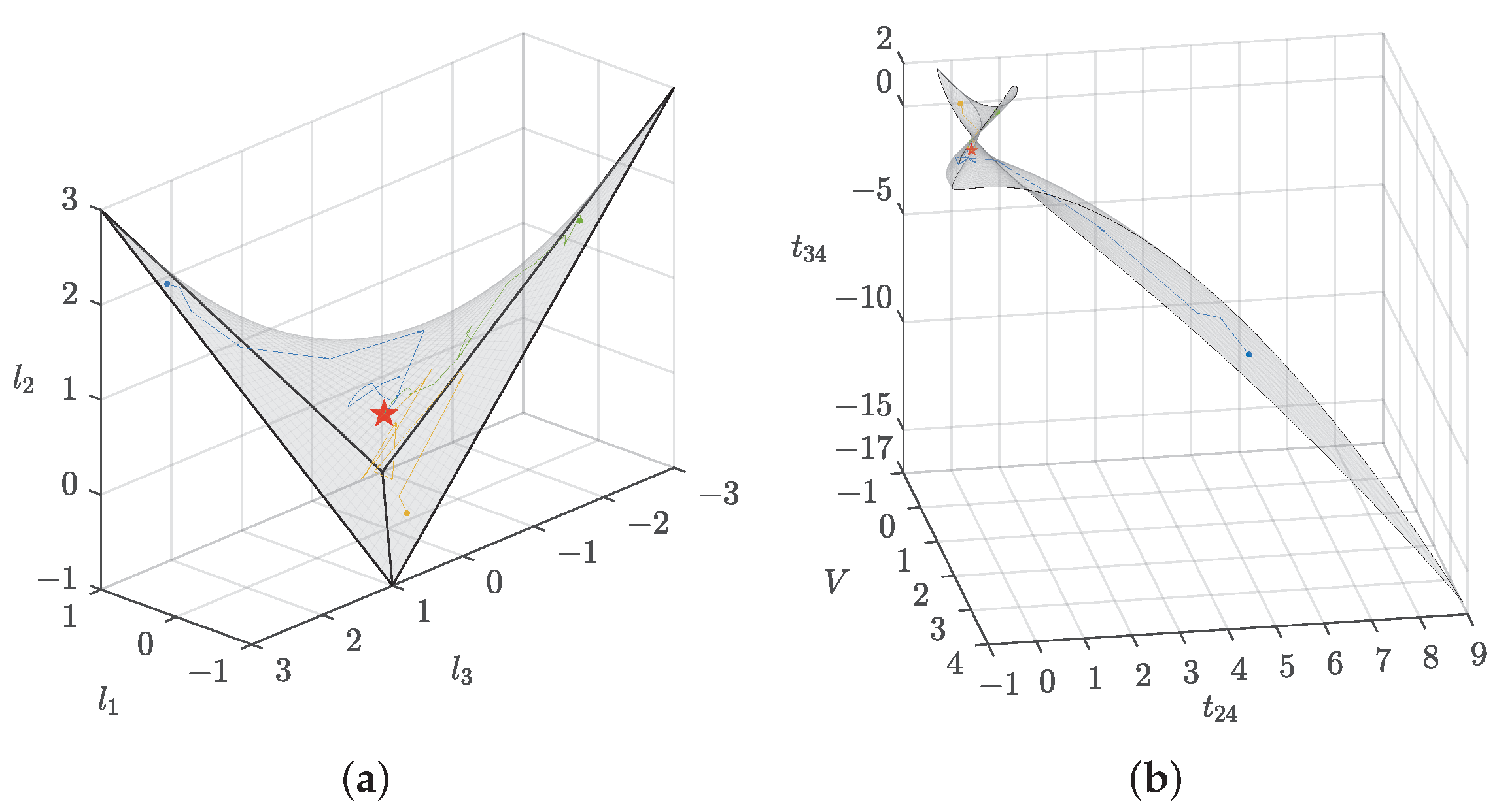
If the condition (8) is satisfied $(t_{24}\ne 12V^2-2V+7/36)$ that there exists a functional optimal observer (4) of the third order solving the optimal filtering problem. In this case, to find unknown variables $(V,t_{24},t_{34}),$ the problem of minimizing the optimality criterion is solved with a restriction on the parameters that must be such that the characteristic polynomial of the observer is stable. Figure 2 illustrates solution of this problem in discrete stability regions given by the inequalities (9) in coordinates $(l_1,l_2,l_3)$ on Figure 2a and in coordinates $(V,t_{24},t_{34})$ on Figure 2b. As one can see, solution paths of the sequential quadratic programming method [41] from different starting points converge to the common minimum of the optimality criterion (4), which has the following coordinates

$$l_1\approx -0.0119,l_2\approx 0.2303,l_3\approx 0.0591;$$

$$V\approx 0.373,t_{24}\approx -0.0636,t_{34}\approx 0.0361.$$

The numerical values of the third-order filter matrices are

$$P=(1\hspace{1em}0\hspace{1em}0),N\approx \left(\begin{array}{ccc}0& 1& 0\\ 0& 0& 1\\ 0.0119& -0.2303& -0.0591\end{array}\right),$$

$$T\approx \left(\begin{array}{cccc}1& 0.5& 0.3333& -0.123\\ 0.5& 0.3333& -0.123& -0.0636\\ 0.3333& -0.123& -0.0636& 0.0361\end{array}\right),M\approx \left(\begin{array}{c}-0.503\\ 0.0776\\ 0.0528\end{array}\right),V\approx 0.373.$$

The optimality criterion in this case is

$$J\approx 2.3179.$$

Thus, the optimality criterion (3) for the third-order filter turned out to be less than for the second-order filter. Previously, second and third order filters were compared from both practical and theoretical points of view. In the context of satellite signal processing, it has been shown [42] that increasing the order of the filters led to an improvement in dynamic stress performance. In [17], a smaller value of the ${\mathcal{H}}_2$ norm for a third-order filter over a second-order filter was obtained on a numerical experiments. Moreover, it has recently been theoretically explained [22] that, as the order of the reduced model was increased, the deviation in the satisfaction of the optimality conditions further reduced.

6. Conclusions

Necessary and sufficient conditions for the existence of discrete unbiased filters of the second and third order are proposed. In the canonical basis, analytical expressions are obtained both for the transfer function matrix of the estimation error system and for the coefficients of the characteristic polynomial of functional filters. In a numerical experiment, filters of the second and third order are constructed for a linear stochastic discrete system of the fourth order. The comparison was carried out according to the root-mean-square optimality criterion. It is shown that, in comparison with the second-order filter, the third-order filter is more optimal in terms of the quadratic criterion in the steady state.

References

1. Stratonovich, R.L. Optimum nonlinear systems which bring about a separation of a signal with constant parameters from noise. Radiofizika 1959, 2, 892–901. [Google Scholar]
2. Stratonovich, R.L. Application of the Markov processes theory to optimal filtering. Radio Eng. Electron. Phys. 1960, 5, 1–19. [Google Scholar]
3. Kalman, R.E. A New Approach to Linear Filtering and Prediction Problems. J. Basic Eng. 1960, 82, 35–45. [Google Scholar] [CrossRef] [Green Version]
4. Kalman, R.E.; Bucy, R.S. New Results in Linear Filtering and Prediction Theory. J. Basic Eng. 1961, 83, 95–108. [Google Scholar] [CrossRef]
5. Luenberger, D. Observers for multivariable systems. IEEE Trans. Autom. Control 1966, 11, 190–197. [Google Scholar] [CrossRef]
6. O’Reilly, J. Observers for Linear Systems; Academic Press: London, UK, 1983. [Google Scholar]
7. Korovin, S.K.; Fomichev, V.V. State Observers for Linear Systems with Uncertainty; de Gruyter: Berlin, Germany, 2009. [Google Scholar]
8. Korovin, S.K.; Il’in, A.V.; Fomichev, V.V.; Hlawenka, A. Asymptotic observers for uncertain vector linear systems. Dokl. Math. 2004, 69, 483–487. [Google Scholar]
9. Korovin, S.K.; Medvedev, I.S.; Fomichev, V.V. Functional observers for linear uncertain stationary dynamical systems. Dokl. Math. 2006, 74, 934–938. [Google Scholar] [CrossRef]
10. Dombrovskij, V.V. Method of synthesizing suboptimal filters of reduced order for digital linear dynamic systems. Autom. Remote Control 1981, 42, 1483–1489. [Google Scholar]
11. Sims, C.S. Reduced-Order Modeling and Filtering. In Advances in Theory and Applications; Control and Dynamic Systems; Leondes, C., Ed.; Academic Press: New York, NY, USA, 1982; Volume 18, pp. 55–103. [Google Scholar] [CrossRef]
12. Dombrovskij, V.V. Synthesis and stability of continuous and discrete low-order linear filters. Autom. Remote Control 1989, 50, 1533–1539. [Google Scholar]
13. Nagpal, K.M.; Helmick, R.E.; Sims, C.S. Reduced-order estimation Part 1. Filtering. Int. J. Control 1987, 45, 1867–1888. [Google Scholar] [CrossRef]
14. Darouach, M. On the optimal unbiased functional filtering. IEEE Trans. Autom. Control 2000, 45, 1374–1379. [Google Scholar] [CrossRef]
15. Darouach, M.; Boutayeb, M.; Zasadzinski, M. Reduced order filtering for stochastic discrete-time systems with unknown inputs. IFAC Proc. Vol. 2002, 35, 133–138. [Google Scholar] [CrossRef]
16. Darouach, M.; Ali, H.S. Optimal unbiased functional filtering in the frequency domain. Syst. Sci. Control Eng. 2014, 2, 308–315. [Google Scholar] [CrossRef] [Green Version]
17. Aalto, H. Simplified Design of H 2 -suboptimal Reduced-order Filters. IFAC Proc. Vol. 2013, 46, 230–235. [Google Scholar] [CrossRef]
18. Singh, S.; Janardhanan, S. Sliding mode control-based linear functional observers for discrete-time stochastic systems. Int. J. Syst. Sci. 2017, 48, 3246–3253. [Google Scholar] [CrossRef]
19. Kamenshchikov, M.A.; Kapalin, I.V. A procedure for constructing optimum functional filters for linear stationary stochastic systems. Mosc. Univ. Comput. Math. Cybern. 2018, 42, 163–170. [Google Scholar] [CrossRef]
20. Fomichev, V.V.; Kamenshchikov, M.A. Comparative analysis of optimal filters of the second and third order for continuous-time systems. Differ. Equ. 2021, 57, 1527–1535. [Google Scholar] [CrossRef]
21. Zulfiqar, U.; Sreeram, V.; Ahmad, M.I.; Du, X. Frequency-weighted H 2 -pseudo-optimal model order reduction. IMA J. Math. Control Inf. 2021, 38, 622–653. [Google Scholar] [CrossRef]
22. Zulfiqar, U.; Sreeram, V.; Ahmad, M.I.; Du, X. Frequency-weighted H 2 -optimal model order reduction via oblique projection. Int. J. Syst. Sci. 2022, 53, 182–198. [Google Scholar] [CrossRef]
23. Simon, D. Reduced order kalman filtering without model reduction. Control Intell. Syst. 2007, 35. [Google Scholar] [CrossRef] [Green Version]
24. Åström, K.J. Introduction to Stochastic Control Theory; Academic Press: New York, NY, USA, 1970. [Google Scholar]
25. Kamenshchikov, M.A. Transfer functions of optimum filters of different dynamic orders for discrete systems. Mosc. Univ. Comput. Math. Cybern. 2021, 45, 60–70. [Google Scholar] [CrossRef]
26. Kwakernaak, H.; Sivan, R. Linear Optimal Control Systems; Wiley-Interscience: New York, NY, USA, 1972. [Google Scholar]
27. Jury, E. A Simplified Stability Criterion for Linear Discrete Systems. Proc. IRE 1962, 50, 1493–1500. [Google Scholar] [CrossRef]
28. Saberi, A.; Stoorvogel, A.A.; Sannuti, P. Filtering Theory; Birkhäuser: Boston, MA, USA, 2007. [Google Scholar]
29. Kailath, T. Linear Systems; Prentice-Hall: Hoboken, NJ, USA, 1980. [Google Scholar]
30. Chen, C.T. Linear System Theory and Design; Oxford University Press: New York, NY, USA, 1999. [Google Scholar]
31. Tsypkin, Y.Z. Sampling Systems Theory and Its Application; Pergamon: Oxford, UK, 1964. [Google Scholar]
32. Jury, E.I. Theory and Application of the z-Transform Method; Wiley: New York, NY, USA, 1964. [Google Scholar]
33. Jury, E. A note on the evaluation of the total square integral. IEEE Trans. Autom. Control 1965, 10, 110–111. [Google Scholar] [CrossRef]
34. Astrom, K.; Jury, E.; Agniel, R. A numerical method for the evaluation of complex integrals. IEEE Trans. Autom. Control 1970, 15, 468–471. [Google Scholar] [CrossRef]
35. Jury, E.; Gutman, S. The inner formulation for the total square integral (sum). Proc. IEEE 1973, 61, 395–397. [Google Scholar] [CrossRef]
36. Greaves, C.; Gagne, G.; Bordner, G. Evaluation of integrals appearing in minimization problems of discrete-data systems. IEEE Trans. Autom. Control 1966, 11, 145–148. [Google Scholar] [CrossRef]
37. James, H.M.; Nichols, N.B.; Phillips, R.S. Theory of Servomechanisms; McGraw-Hill: New York, NY, USA, 1947. [Google Scholar]
38. Popov, E.P. The Dynamics of Automatic Control Systems; Pergamon: Oxford, UK, 1962. [Google Scholar]
39. Jury, E.; Dewey, A. A general formulation of the total square integrals for continuous systems. IEEE Trans. Autom. Control 1965, 10, 119–120. [Google Scholar] [CrossRef]
40. Man, F. Evaluation of time-weighted quadratic performance indices for linear discrete systems. IEEE Trans. Autom. Control 1970, 15, 496–497. [Google Scholar] [CrossRef]
41. Nocedal, J.; Wright, S. Numerical Optimization; Springer Science & Business Media: New York, NY, USA, 2006. [Google Scholar]
42. Kaplan, E.; Hegarty, C. Understanding GPS: Principles and Applications; Artech House: Boston, MA, USA, 2005. [Google Scholar]
Figure 1. Graph of the function (17). The global minimum of the function J ( V ) over the open interval ( 1 / 36 , 13 / 108 ) is the red point ( V 0.1148 , J ( V ) 4.1223 ). The two blue dashed lines are the asymptotes V = 1 / 36 and V = 13 / 108 .
Mathematics 10 00370 g001
Figure 2. Three convergence paths (blue, green and orange arrows) to the common minimum (red star) of the optimality criterion J from various starting points in the discrete stability regions in coordinates (a) l 1 , l 2 , l 3 ; (b) V , t 24 , t 34 .
Mathematics 10 00370 g002