Abstract
In this work, the quantized Hill problem is considered in order for us to study the existence and stability of equilibrium points. In particular, we have studied three different cases which give all whole possible locations in which two points are emerging from the first case and four points from the second case, while the third case does not provide a realistic locations. Hence, we have obtained four new equilibrium points related to the quantum perturbations. Furthermore, the allowed and forbidden regions of motion of the first case are investigated numerically. We demonstrate that the obtained result in the first case is a generalization to the classical one and it can be reduced to the classical result in the absence of quantum perturbation, while the four new points will disappear. The regions of allowed motions decrease as the value of the Jacobian constant increases, and these regions will form three separate areas. Thus, the infinitesimal body can never move from one allowed region to another, and it will be trapped inside one of the possible regions of motion with the relative large values of the Jacobian constant.
MSC:
70F05; 70F07; 70F10; 70F15; 70H14
1. Introduction
Hill’s problem is a particularly limiting case for the restricted three-body problem (RTBP). Researchers can obtain the Hill problem by using some scales and transformations while taking limits, as mass parameter tends to zero. Hence, it is an interesting application based problem, and many scientists have studied different versions of this problem by considering different perturbation forces in the classical Hill problem. This means the primary bodies possess point masses and move in circular orbits around their common centre of mass or in elliptical trajectory, while the third body moves in space under the effect of gravitational forces of the primary bodies without affecting their motions [1,2,3,4].
In [5], the authors have studied the Hill stability of satellites by utilising the RTBP configuration. However, in [6,7,8], the authors have studied the same configuration with various perturbations as radiation pressure and oblateness of the primaries. Additionally, in [9,10,11,12], the authors have explored and analysed the Hill four bodies problem with its application to the Earth–Moon–Sun system and satellite motion about binary asteroids. In this context, Hill’s problem, with oblate secondary in three dimensions, has been illustrated in [13], where the equilibrium points and their stability have been determined.
Further to the precedent work, the radiation pressure effect of the bigger primary and the secondary oblateness on the new version of Hill’s problem are investigated in [14], where the authors illustrated that their study is more appropriate for astronomical application. They also used iterative methods to identify the locations of equilibrium points and used the linear stability analysis method to examine their stability properties. They proved that all the equilibrium points are unstable for this model. In [15], the authors investigated Hill’s problem because space missions required the knowledge of orbits with some properties, where periodic solutions are illustrated numerically due to the non-integrability of this problem.
With the continuous contributions analysing the Hill body problem, the existence of positions and stability of collinear equilibrium points in its generalized version under radiation pressure and oblateness effects are studied in [16]; the authors also performed the basins of attraction through the Newton–Raphson method for many values of used parameters. Furthermore, in [17] the author investigated the basins of convergence in the aforementioned problem; his numerical analysis revealed the extraordinary and beautiful formations on the complex plane. In [18], the authors have performed the Hill’s problem by assuming the primaries as the source of radiation pressure; they have determined the asymptotic orbits at collinear points and the same to the lyapunov periodic orbits.
The spatial or planar restricted three-body problem (RTBP) under any kind of perturbation is called the perturbed model. Otherwise, it can be called the phot–gravitational, relativistic, or quantized problem in the case that the system is analysed under the effect of radiation pressure, relativistic, or quantum corrections perturbation, respectively [19,20,21,22,23]. The analysis of the spatial quantized RTBP (i.e., the spatial of RTBP under the effect of quantum corrections) is studied in [24], where the locations of equilibrium points and the allowed and forbidden regions of motions are examined. Furthermore, the quantized RTBP is developed to construct a new version of the Hill problem [25], where the equations of motion for the Hill problem are evaluated under the quantum corrections. Thus, the obtained system is called quantized Hill problem (QHP).
Recently, in [26], the authors investigated the Hill’s problem by assuming that the infinitesimal body varies its mass according to Jeans law, they investigated numerically the location of equilibrium points, regions of motion, and basins of attraction and also examined the stability status of these points by using Meshcherskii’s space–time transformation. Furthermore, in [27] the authors investigated the differences and similarities among the classical perturbation theory, Poincaré–Lindstedt technique, multiple scales method, the KB averaging method, and averaging theory, while the latter is used to find periodic orbits in the framework of the spatial QHP. They stated that this model can be utilized to develop a lunar theory and families of periodic orbits.
In the framework of RTBP, which can be reduced to the Hill model, some effective contributions are outlined in [28,29,30], where the effects of lack of sphericity body shape and radiation pressure on the primaries are studied. In addition, the effect of mass variation in the frame of RTBP is investigated in [31,32,33,34], where the authors have also studied the impact of these perturbations on the positions of equilibrium points, Poincaré surfaces of section, regions of possible and forbidden motion, and basins of attraction and examined the stability of these equilibrium points such that it is proven that, in most cases, these points are unstable.
In general, the Hill body problem has a great significance in both stellar and solar systems and in dynamical astronomy; it has received a considerable analysis in its own literature. Primarily, it is formulated as a model to analyse the Moon’s motion around the Earth under the effect of Sun perturbation. Furthermore, its model, with simple modifications, can also serve as a model for the motion of a star in a star cluster under the created perturbations from the galaxy. The importance of this problem motivated us to study and analyse the Hill body problem under the perturbation of quantum corrections.
In this work, the QHP is considered to study the existence of equilibrium points alongside examining their stability. Under the effect of quantum corrections, the locations of equilibrium points have been analysed. In particular, we have studied three different cases which give all possible locations, where two points are emerging from the first case and they are considered a generalization for the classical two points, as well as four points from the second case, while the third case does not provide any realistic locations. Hence, we have obtained four new equilibrium points related to the quantum perturbations. Furthermore, We demonstrate that the obtained result in the first case can be reduced to the classical result, while the four new points will disappear in the absence of quantum perturbation.
The paper is organized in six sections as follows: The literature surrounding the problem is given in Section 1. The equations of motion are preformed in Section 2. In Section 3, we have determined the positions of equilibrium points. The stability of equilibrium points are studied in Section 4. Furthermore, the numerical results are estimated in Section 5. Finally, the conclusion of the work is presented in Section 6.
2. Equations of Motion
Following the same notations and procedure in [25], we can write the equations of motion of the quantized Hill problem in the synodic coordinates system as:
where
and
In System (1), the parameters , , and represent very small amounts with order of , but is of order where c is the speed of light. Therefore, the value of will tends to zero [27]. Hence . In this context, System (1) can be rewritten as:
where
We would like to provide the reader with the following investigations about the aforementioned perturbation parameters. In fact, the parameters , , and identify the size of the relativistic effect, while estimates the quantum correction contribution. However, all of these effects tend to zero in the case of large distances [21,35].
3. Analysis of Equilibrium Points
The equilibrium points can be obtained by equating all the derivatives with respect to time by zero in system (5), hence
In the classical case, we mean that the quantum effect will be neglected, the parameter , then the equilibrium points are given by where and , hence .
To find the equilibrium points under the quantized effect ( and ), we have to find the solutions of System (6); there are some cases which can be applied to analyse the solutions of this system.
- First case:
- , then , and .
In this case, one obtains
Equation (7) gives a quintic equation in the following form
The solution of the fifth degree equation is generally too complicated, however the equation has at least one real root. Instead, numerical approximations can be evaluated using a root-finding algorithm for polynomials.
In fact, it is not our aim to find a solution of a quintic equation, but we aim to find the quantum corrections’ impact on the locations of equilibrium points. Thus, we impose that , where is a very small quantity which embodies the effect of quantum correction on the locations of equilibrium points after substituting into Equation (7) or Equation (8), keeping all terms with coefficients of and only, and neglecting all terms with an order of or more. Hence, will satisfy two values, and , which are given by
Substituting in Equation (9), one obtains
As and are very small quantities with order of and , respectively, we keep only terms with order of and and neglect the remanning terms. Thereby, the approximated values of the perturbed parameter are governed by
The parameter of embodies the effect of the quantum corrections and it must equal zero in the absence of these corrections, i.e., when and . However, the obtained solution of does not equal zero and gives an inconvenient solution; thus, the value of is rejected. Hence, the proper approximated value of the parameter is given by
Utilizing Equation (10) with relation to , then the distance at the quantized equilibrium point is
As , we have two possible values for x and , . Thus, the quantized equilibrium points are and , which is considered a generalization of the classical case and can be reduced to the classical one when and .
- Second case:
- , then , and .
This case could occur when the parameters of quantum corrections are negative, i.e., the values of and are negative [24]. Hence, when the solutions of the following quadratic equation are possible
The possible solutions of Equation (14) are
The solutions in Equation (15) are valid if the values of and are positive. To investigate this property, first we remark that , , and have values with order of , , and . Then, the approximated series solutions of Equation (15) can be written as
It is clear that from Equation (16) the values of and are very small and positive when and , respectively, take negative values. Then, we have four new equilibrium points corresponding to the second case under the perturbation of quantum corrections, where and . The new four points are , , , and
- Third case:
- , then , and .
In this case, one obtains
Equation (17) gives also a quintic equation in the following form
To find the solution of Equation (18), we impose that , where is very small quantity which embodies the effect of quantum correction on the locations of equilibrium points in the current case after substituting into Equation (18) and keeping all terms with coefficients of and only, neglecting all terms with order of or more. Hence, will satisfy two values, and , which are given by
It is clear that from Equation (19) the obtained values of the perturbation parameter is complex, which mean that the assumption of the third case does not lead to realistic situations. Thus, this case does not give real equilibrium points and it is rejected.
4. Stability Status of Equilibrium Points
Next, to check the equilibrium points stability, we have to write the equations of motion in to phase space. Thus, System (5) can be rewritten in the following form
where
Here, the Jacobian integral can be rewitten as
The motion in the proximity of any of the equilibrium points and can be studied by putting , and in Equations (20) and (21). Then, we can rewrite the equations of motion in the phase space as
where the superscript zero means that the second derivatives of H are evaluated at the related equilibrium point.
We will examine the stability of equilibrium points in two cases only because there are no equilibrium points in the third case.
4.1. First Case
In this case the equilibrium points and are in symmetry about the Y-axis, therefore it is enough to examine the stability of only one of these two points. In this context, we have to evaluate the values of corresponding to , which are as follows:
Here, , , and show that the sign changes occur one at a time time, thus there exists at least one positive real root. Therefore, the equilibrium point will be unstable in this case.
4.2. Second Case
In this case, the equilibrium points and are symmetrical about the X-axis, hence it is sufficient to examine the stability of only two of these four points. Additionally, we have to evaluate the values of and , and 5 corresponding to and , which are as follows:
and
Here, , , , and , where , show that the sign changes occur one at a time, thus there exists at least one positive real root. Therefore, the equilibrium point will be unstable in this case.
5. Numerical Results
In this section, we illustrate some dynamical properties numerically for the proposed system (i.e., the quantized Hill system) such as the equilibrium points and the allowed and forbidden regions of motion under the quantum corrections. In order to avoid the reparation, we will present the numerical analysis on the first case of equilibrium points; the same procedure can be carried out for the second case.
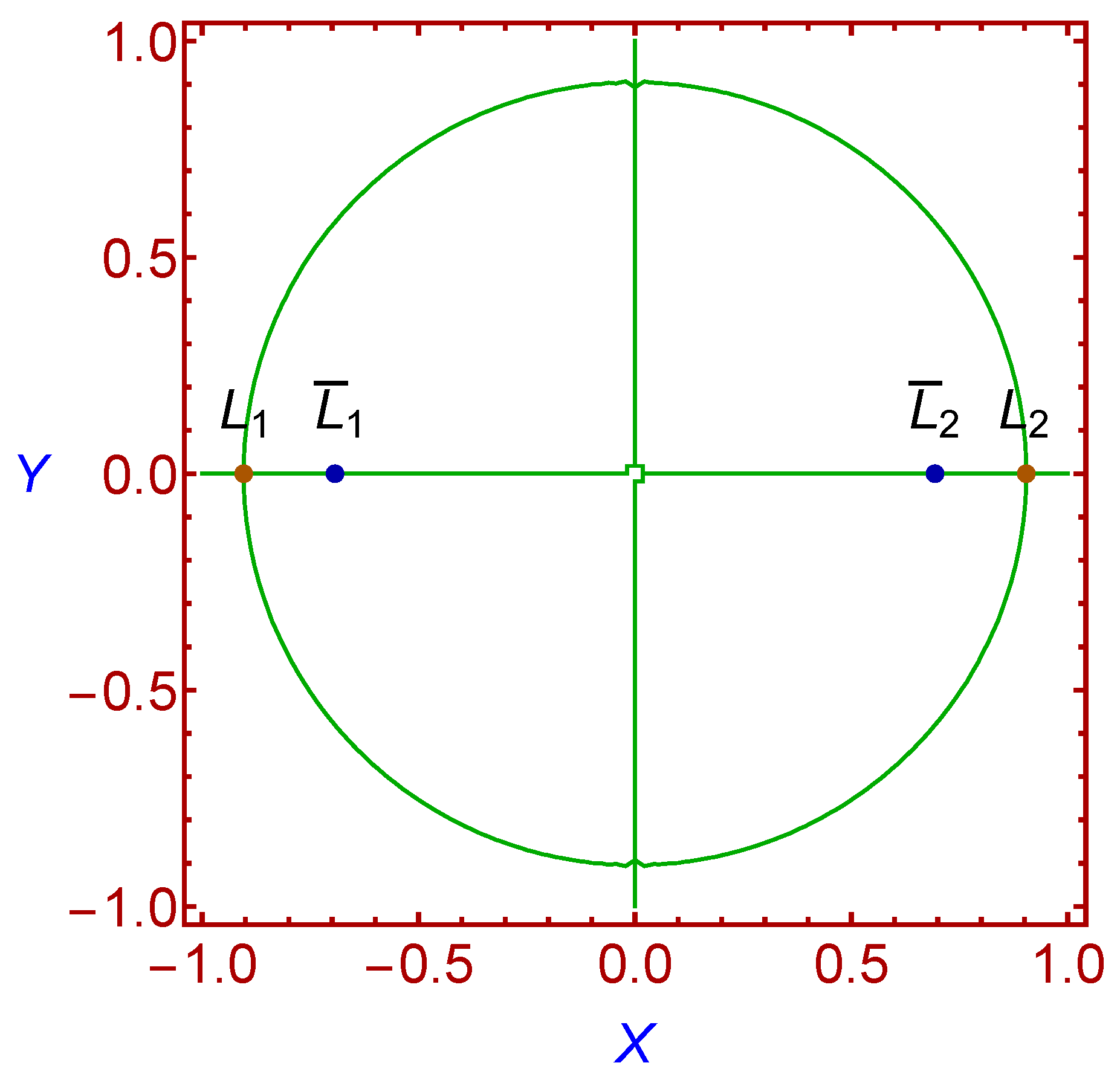
The locations of equilibrium points are shown in Figure 1, for which we have taken zero as the derivatives with respect to time in Equation (5). Then, with the help of the well-known Mathematica Software, the collinear equilibrium points and under the quantum corrections, as well as the unperturbed equilibrium points and , are estimated numerically. Both points exist either side of the origin on the X-axis and are in symmetry about Y-axis. However, we mark that the distance between the perturbed points is more than the distance between the unperturbed points. Of course, this perturbation will affect the other dynamical properties.
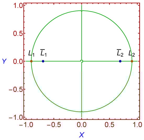
Figure 1.
Locations of equilibrium points.
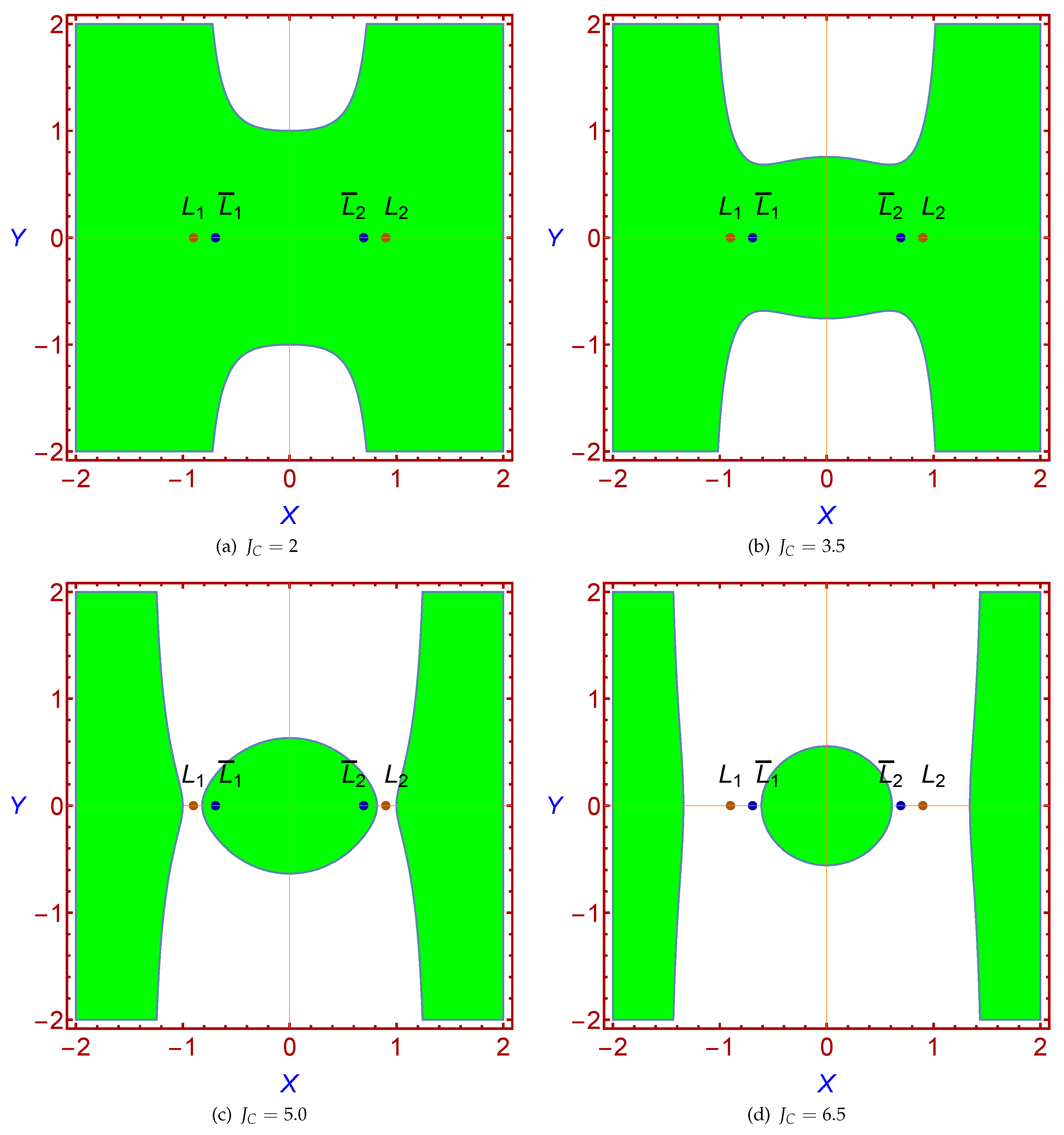
One of the most dynamical properties which can be identified by the Jacobian integral is the possible and forbidden regions of infinitesimal body motions, which are restricted to the locations of where v is the velocity of the infinitesimal body. Hence, Equation (22) can be used to determine the allowed or forbidden regions of motions, as in Figure 2, where the coloured green areas identify the regions of possible motions, while the white determine forbidden regions.
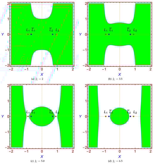
Figure 2.
Regions of allowed (green area) and forbidden (white area) motion.
It is clear from Figure 2a that when the Jacobian constant is relatively small there is one large area for possible region of motion, and the body could move from any region point to another (or from () to ()). When becomes larger, the forbidden region is extended, as in Figure 2b. With further increase in the value of , the forbidden region becomes larger, while the possible region of motion forms three septate areas starting from the perturbed equilibrium points and , as in Figure 2c. In addition, the body cannot move from one to another, because the three areas are not connected. With further increase in the value of , the inner and two outer regions decrease while the separate areas start from the unperturbed equilibrium points and , as in Figure 2d. We remark that the infinitesimal can never move from one allowed region to another, and the body will be trapped inside one of the possible regions of motion with the relative large values of the Jacobian constant, as in the case of Figure 2c,d.
The condition of does not provide information about the size or shape of the orbit or the trajectory of the body; it can only identify the region where the infinitesimal body could move.
6. Conclusions
In this work, the quantized Hill problem is considered to study the existence of equilibrium points alongside examining their stability. Under the effect of quantum corrections, the locations of equilibrium points have been analysed, we have studied three different cases which give all possible locations, where two points emerge from the first case, taking a place on the X-axis, and four points dos so from the second case and lie on Y-axis. The third case does not provide a realistic location. Hence, we have obtained four new equilibrium points related to the quantum perturbations.
In this context, we have tested the stability status of all of the equilibrium points and we have found that all points are unstable. Further, we have illustrated the locations of equilibrium points for the first case and the related allowed regions of motion numerically. Similarly, we can perform these illustrations for the second case. Here, we found two equilibrium points which are either side of the origin on the X-axis and in symmetry about the Y-axis, as in Figure 1. The regions of possible and forbidden motion are investigated for different values of Jacobian constant, as in Figure 2.
Finally, we demonstrate that the obtained result in the first case is a generalization of the classical one, and it can be reduced to the classical result, while the four new points will disappear in the absence of quantum perturbation. The regions of possible motions decrease with the increasing value of Jacobian constant and these regions will form three separate areas. Thus, the infinitesimal body can never move from one allowed region to another, and it will be trapped inside one of the possible regions of motion with the relative large values for the Jacobian constant.
Author Contributions
Formal analysis, A.A.A., S.A., E.I.A. and S.K.S.; investigation, A.A.A., S.A., E.I.A. and S.K.S.; methodology, A.A.A., S.A., E.I.A. and S.K.S.; project administration, E.I.A.; software, E.I.A.; Validation, A.A.A., S.A., E.I.A. and S.K.S.; visualization, E.I.A.; Writing—original draft, E.I.A.; and writing—review and editing, A.A.A., S.A., E.I.A. and S.K.S. All authors have read and agreed to the published version of the manuscript.
Funding
This work was funded by the National Research Institute of Astronomy and Geophysics (NRIAG), Helwan 11421, Cairo, Egypt. The third author, therefore, acknowledges his gratitude for NRIAG’s technical and financial support. Moreover, this paper was supported by the National Natural Science Foundation of China (NSFC), grant no. 12172322.
Institutional Review Board Statement
Not applicable.
Informed Consent Statement
Not applicable.
Data Availability Statement
The study does not report any data.
Conflicts of Interest
The authors declare no conflict of interest.
References
- Kummer, M. On the stability of Hill’s solutions of the plane restricted three body problem. Am. J. Math. 1979, 101, 1333–1354. [Google Scholar] [CrossRef]
- Perdiou, A.; Perdios, E.; Kalantonis, V. Periodic orbits of the Hill problem with radiation and oblateness. Astrophys. Space Sci. 2012, 342, 19–30. [Google Scholar] [CrossRef]
- Makó, Z. Connection between Hill stability and weak stability in the elliptic restricted three-body problem. Celest. Mech. Dyn. Astron. 2014, 120, 233–248. [Google Scholar] [CrossRef]
- Gong, S.; Li, J. Analytical criteria of Hill stability in the elliptic restricted three body problem. Astrophys. Space Sci. 2015, 358, 1–10. [Google Scholar] [CrossRef]
- Szebehely, V. Stability of artificial and natural satellites. Celest. Mech. 1978, 18, 383–389. [Google Scholar] [CrossRef]
- Markellos, V.V.; Roy, A.E. Hill stability of satellite orbits. Celest. Mech. 1981, 23, 269–275. [Google Scholar] [CrossRef]
- Markellos, V.V.; Roy, A.E.; Velgakis, M.J.; Kanavos, S.S. A photogravitational Hill problem and radiation effects on Hill stability of orbits. Astrophys. Space Sci. 2000, 271, 293–301. [Google Scholar] [CrossRef]
- Markellos, V.V.; Roy, A.E.; Perdios, E.A.; Douskos, C.N. A Hill problem with oblate primaries and effect of oblateness on Hill stability of orbits. Astrophys. Space Sci. 2001, 278, 295–304. [Google Scholar] [CrossRef]
- Scheeres, D. The Restricted Hill Four-Body Problem with Applications to the Earth-Moon-Sun System. Celest. Mech. Dyn. Astron. 1998, 70, 75–98. [Google Scholar] [CrossRef]
- Scheeres, D.J.; Bellerose, J. The Restricted Hill Full 4-Body Problem: Application to spacecraft motion about binary asteroids. Dyn. Syst. Int. J. 2005, 20, 23–44. [Google Scholar] [CrossRef]
- Burgos-García, J.; Gidea, M. Hill’s approximation in a restricted four-body problem. Celest. Mech. Dyn. Astron. 2015, 122, 117–141. [Google Scholar] [CrossRef] [Green Version]
- Liu, C.; Gong, S. Hill stability of the satellite in the elliptic restricted four–body problem. Astrophys. Space Sci. 2018, 363, 1–9. [Google Scholar] [CrossRef]
- Perdiou, A.E.; Markellos, V.V.; Douskos, C.N. The Hill problem with oblate secondary: Numerical Exploration. Earth Moon Planets 2006, 97, 127–145. [Google Scholar] [CrossRef]
- Markakis, M.P.; Perdiou, A.E.; Douskos, C.N. The photogravitational Hill problem with oblateness: Equilibrium points and Lyapunov families. Astrophys. Space Sci. 2008, 315, 297–306. [Google Scholar] [CrossRef]
- Batkhin, A.B.; Batkhina, N.V. Hierarchy of periodic solutions families of spatial Hills problem. Sol. Syst. Res. 2009, 43, 178. [Google Scholar] [CrossRef]
- Douskos, C.N. Collinear equilibrium points of Hill’s problem with radiation pressure and oblateness and their fractal basins of attraction. Astrophys. Space Sci. 2010, 326, 263–271. [Google Scholar] [CrossRef]
- Zotos, E.E. Comparing the fractal basins of attraction in the Hill problem with oblateness and radiation. Astrophys. Space Sci. 2017, 362, 190. [Google Scholar] [CrossRef] [Green Version]
- Kalantonis, V.S.; Perdiou, A.E.; Douskos, C.N. Asymptotic orbits in Hills problem when the larger primary is a source of radiation. Appl. Nonlinear Anal. 2018, 134, 523–535. [Google Scholar]
- Nartikoev, P. Photogravitational Restricted Three-Body Problem; Sev.-Oset. Univ.: Ordzhonikidze, Russia, 1987. [Google Scholar]
- Ragos, O.; Perdios, E.; Kalantonis, V.; Vrahatis, M. On the equilibrium points of the relativistic restricted three-body problem. Nonlinear Anal. Theory Methods Appl. 2001, 47, 3413–3418. [Google Scholar] [CrossRef]
- Mohr, R.; Furnstahl, R.; Hammer, H.W.; Perry, R.; Wilson, K. Precise numerical results for limit cycles in the quantum three-body problem. Ann. Phys. 2006, 321, 225–259. [Google Scholar] [CrossRef] [Green Version]
- Donoghue, J.F. Leading quantum correction to the Newtonian potential. Phys. Rev. Lett. 1994, 72, 2996. [Google Scholar] [CrossRef] [PubMed] [Green Version]
- Battista, E.; Esposito, G. Restricted three-body problem in effective-field-theory models of gravity. Phys. Rev. D 2014, 89, 084030. [Google Scholar] [CrossRef] [Green Version]
- Alshaery, A.; Abouelmagd, E.I. Analysis of the spatial quantized three-body problem. Results Phys. 2020, 17, 103067. [Google Scholar] [CrossRef]
- Abouelmagd, E.I.; Kalantonis, V.S.; Perdiou, A.E. A Quantized Hill’s Dynamical System. Adv. Astron. 2021, 2021, 9963761. [Google Scholar] [CrossRef]
- Bouaziz, F.; Ansari, A.A. Perturbed Hill’s problem with variable mass. Astron. Nachr. 2021, 342, 666–674. [Google Scholar] [CrossRef]
- Abouelmagd, E.I.; Alhowaity, S.; Diab, Z.; Guirao, J.L.; Shehata, M.H. On the Periodic Solutions for the Perturbed Spatial Quantized Hill Problem. Mathematics 2022, 10, 614. [Google Scholar] [CrossRef]
- Abouelmagd, E.I.; El-Shaboury, S.M. Periodic orbits under combined effects of oblateness and radiation in the restricted problem of three bodies. Astrophys. Space Sci. 2012, 341, 331–341. [Google Scholar] [CrossRef]
- Abouelmagd, E.I.; Mostafa, A. Out of plane equilibrium points locations and the forbidden movement regions in the restricted three-body problem with variable mass. Astrophys. Space Sci. 2015, 357, 58. [Google Scholar] [CrossRef]
- Ansari, A.A. Triaxial primaries in circular Hill problem. Astron. Rep. 2021, 65, 1178–1183. [Google Scholar] [CrossRef]
- Singh, J.; Leke, O. Equilibrium points and stability in the restricted three-body problem with oblateness and variable masses. Astrophys. Space Sci. 2012, 340, 27–41. [Google Scholar] [CrossRef]
- Ansari, A.A. Effect of Albedo on the motion of the infinitesimal body in circular restricted three-body problem with variable masses. Ital. J. Pure Appl. Math. 2017, 38, 581–600. [Google Scholar]
- Abouelmagd, E.I.; Ansari, A.A.; Ullah, M.S.; Guirao, J.L.G. A Planar Five-body Problem in a Framework of Heterogeneous and Mass Variation Effects. Astron. J. 2020, 160, 216. [Google Scholar] [CrossRef]
- Suraj, M.S.; Aggarwal, R.; Asique, M.C.; Mittal, A. On the modified circular restricted three-body problem with variable mass. New Astron. 2021, 84, 101510. [Google Scholar] [CrossRef]
- Bjerrum-Bohr, N.E.J.; Donoghue, J.F.; Holstein, B.R. Quantum gravitational corrections to the nonrelativistic scattering potential of two masses. Phys. Rev. D 2003, 67, 084033. [Google Scholar] [CrossRef] [Green Version]
Publisher’s Note: MDPI stays neutral with regard to jurisdictional claims in published maps and institutional affiliations. |
© 2022 by the authors. Licensee MDPI, Basel, Switzerland. This article is an open access article distributed under the terms and conditions of the Creative Commons Attribution (CC BY) license (https://creativecommons.org/licenses/by/4.0/).