Stochastic Transcription with Alterable Synthesis Rates

Abstract

Background: Gene transcription is a random bursting process that leads to large variability in mRNA numbers in single cells. The main cause is largely attributed to random switching between periods of active and inactive gene transcription. In some experiments, it has been observed that variation in the number of active transcription sites causes the initiation rate to vary during elongation. Results: We established a mathematical model based on the molecular reaction mechanism in single cells and studied a stochastic transcription system consisting of two active states and one inactive state, in which mRNA molecules are produced with two different synthesis rates. Conclusions: By calculation, we obtained the average mRNA expression level, the noise strength, and the skewness of transcripts. We gave a necessary and sufficient condition that causes the average mRNA level to peak at a limited time. The model could help us to distinguish an appropriate mechanism that may be employed by cells to transcribe mRNA molecules. Our simulations were in agreement with some experimental data and showed that the skewness can measure the deviation of the distribution of transcripts from the mean value. Especially for mature mRNAs, their distributions were almost able to be determined by the mean, the noise (or the noise strength), and the skewness.

1. Introduction

The process of synthesizing a ribonucleic acid (RNA) copy of a deoxyribonucleic acid (DNA) molecule is called transcription, which is involved in virtually all significant physiological processes and necessary for all forms of life. It is now well established that transcription is a complex and stochastic process and occurs in a bursting fashion both in prokaryotes [1,2] and eukaryotes [3,4]. From RNA polymerase binding at the promoter to RNA splicing and processing, numerous successive steps are involved in this process, and each one is stochastic. The accumulation of stochasticity in the whole transcription event results in fluctuations in transcripts in single cells.

In the last three decades, experimental works and theoretical works have interacted and helped to move each other forward. Bartman et al. [5] showed that transcriptional burst initiation and polymerase pause release could regulate transcription together. The enhancer and transcription factors regulate transcriptional outputs by modulating the transcriptional burst or frequency [6,7]. Many novel models have been established and used to interpret experimental phenomena. Peccoud and Ycart [8] established a two-state gene expression model in which the promoter stochastically switches between an OFF and an ON state. Tang [9] constructed a three-state model by dividing the OFF state into two substates to evaluate the dynamical and stationary mean transcript level. Cao et al. [10] studied the effect of RNA polymerase recruitment and polymerase pause release and derived the distributions of mRNA and protein numbers. At the same time, many effective approaches have been developed to calculate the distributions of mRNAs and proteins. For instance, Sun et al. [11] and Zhu et al. [12] derived the distribution of mRNA molecules produced in a system activated by cross-talking pathways. Chen and Jiao [13] presented an approach to calculating mRNA distribution with time. Cao and Grima [14] extended the two-state transcription model to dividing cells. Distributions of mRNAs and proteins in a complex expression system were studied in [15,16].

The mRNA production rates always have global effects on RNA synthesis and should play a role in transcription. For example, in dividing cells, the mRNA production rate depends on the cell size and gene copies [17]. The average mRNA level does not double between the interphase and the mitotic phase, and the noise and noise strength depend on the cell cycle duration [18]. Jiao and Tang [19] proposed a novel index, which relates to the transcription level and the noise, to quantify transcription noise’s impact on cell fate commitment. When the production rate was periodic with a fixed period, the average mRNA and the noise were derived [20].

With the development of observation techniques, large amounts of data on gene expression can be measured and collected everyday. However, an increasing amount of data demonstrate that bursting kinetics are highly gene-specific [4,21]. Thus, we should seek to develop a suitable mathematical model to explore the transcription mechanisms of the targeted gene.

Using single-molecule fluorescence in situ hybridization (smFISH), Senecal et al. [6] quantified the transcriptional activity of the protooncogene c-Fos and measured the nascent and mature c-Fos mRNA amounts. They found that several transcriptions after different levels of serum induction showed similar induction kinetics; that is, mRNA levels increased rapidly to reach a maximum and then returned to basal expression after 1∼2 h. Moreover, we can clearly see that the distributions of nascent and mature mRNAs are positively skewed. To understand the molecular mechanisms of the experimental phenomenon reported by Senecal et al. [6], we modify and analyze the two-ON transcription model that they introduced in their paper, and we derive the temporal profiles of the average mRNA level and the mRNA distribution.

In this paper, we describe the two-ON transcription model, detailed in Section 2. The transcriptional output and stochasticity are often quantified by the mean and the noise strength. To depict the distribution of transcripts in more detail, we introduce the skewness to describe the asymmetry of such distribution. For a random variable X, $\mathbf{E}\left[X\right]$ denotes the mean value, while the noise strength and the skewness are defined by

$$\begin{array}{c}\hfill \varphi \left[X\right]=\frac{{\sigma }^2\left[X\right]}{\mathbf{E}\left[X\right]}\mathrm{and}S\left[X\right]=\frac{\rho \left[X\right]}{{\sigma }^3\left[X\right]}\end{array}$$

where ${\sigma }^2\left[X\right]$ and $\rho \left[X\right]$ denote the second and the third central moments, respectively. Since ${\sigma }^2\left[X\right]$ and $\rho \left[X\right]$ are determined by the first to the third raw moments, we only need to calculate $\mathbf{E}\left[X\right],\mathbf{E}\left[X^2\right]$ and $\mathbf{E}\left[X^3\right]$. Thus, we present the master equations of the transcription system and the differential equations of the three moments in Section 2. We show the analytical form of the average mRNA level and give a necessary and sufficient condition such that the average level could peak at a limited time point in Section 3. Moreover, we give a detailed procedure to calculate the skewness but do not present the exact form for the sake of brevity. By using the measured experimental data in [6], we simulate our results in Section 4 and identify more potential properties of the distribution from the skewness by the simulations.

2. Model Specification

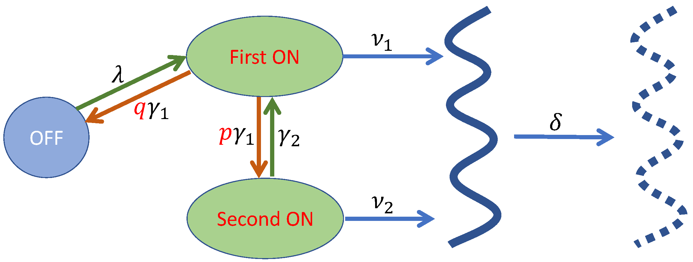
2.1. The Characterization of the Gene Transcription Mechanism

The model is established based on the experimental observations in [6]. When analyzing the serum induction data, Senecal et al. [6] found that there is a temporary increase in the initiation rate during elongation. They conjectured that there may exist a second active state with a higher initiation rate. The experimental phenomenon differs from other models, and the data or parameters cannot be fitted by existing models. This observation motivates us to study the stochastic dynamics of gene transcription with the existence of two active states in detail, and give the analytical form of the average mRNA level and the distribution of transcripts.

We assume that there are two active states with different initiation rates to produce mRNA molecules and one inactive state with no production taking place. As shown in Figure 1, it can be postulated that the gene promoter randomly transfers within the OFF state, the first ON state, and the second ON state with constant rates. To activate transcription, it takes an exponentially distributed time of rate $\lambda$ to open the DNA duplex to form a transcription bubble and bind an RNA polymerase to a special region. The RNA chain is synthesized with synthesis rate ${\nu }_1$ when the RNA polymerase moves along the DNA. The sojourn time in the first ON state is assumed to be independently and exponentially distributed with a rate ${\gamma }_1$. As observed in [6], a second ON state with an independent initiation rate ${\nu }_2$ is added that can be reached at high p-ERK levels from the first ON state, and the system resides at this state for a time, which is independently and exponentially distributed with a rate ${\gamma }_2$. Following such an observation, we assume that, at the exit of the first ON state, the promoter may transfer to the second ON state with a probability p, or to the OFF state with a probability $q=1-p$. At the exit of the second ON state, the promoter returns to the first ON state. Then, the promoter makes a selection again, similar to the previous instance. When the RNA polymerase dissociates at a terminator site, the transcription stops and the DNA duplex reforms. The promoter returns to the OFF state. Throughout the whole transcription process, transcripts are turned over with a degradation rate $\delta >0$.

As is common, we use the mean, the noise strength to depict the average transcription level, and the fluctuation of transcripts in single cells. Let $M\left(t\right)$ denote the transcript number of a gene of interest in single cells at time t. In individual cells, $M\left(t\right)$ is a natural number that varies over a large region. Usually, we expect to count the average transcript number produced per cell in a population of isogenic cells. This value, called the mean, is given by the first moment of $M\left(t\right)$, i.e.,

$$\begin{array}{c}\hfill m\left(t\right)=\mathbf{E}\left[M\right(t\left)\right].\end{array}$$

To determine the numbers of transcripts in individual cells deviating from the mean, we employ the noise strength, defined by

$$\begin{array}{c}\hfill \varphi \left(t\right)=\mathbf{E}\left[\frac{{[M\left(t\right)-m\left(t\right)]}^2}{m\left(t\right)}\right]=\frac{{\sigma }^2\left(t\right)}{m\left(t\right)}=\frac{\mu \left(t\right)-m^2\left(t\right)}{m\left(t\right)},\end{array}$$

to characterize the fluctuation of transcripts, where $\mu \left(t\right)=\mathbf{E}\left[M^2\left(t\right)\right]$ is the second moment of transcripts. Furthermore, we also introduce the probability mass function$P_m\left(t\right)$, defined by

$$\begin{array}{c}\hfill P_m\left(t\right)=\mathrm{Prob}\{M\left(t\right)=m\}\end{array}$$

to show the distribution of transcripts.

To better depict the distribution $P_m\left(t\right)$, we introduce the skewness of transcripts, which is defined as

$$\begin{array}{c}\hfill S\left(t\right)=\mathbf{E}{\left[\frac{M\left(t\right)-m\left(t\right)}{\sigma \left(t\right)}\right]}^3=\frac{k_3\left(t\right)-3\mu \left(t\right)m\left(t\right)+2m^3\left(t\right)}{{\sigma }^3\left(t\right)},\end{array}$$

where $k_3\left(t\right)=\mathbf{E}\left[M^3\left(t\right)\right]$ is the third moment of transcripts. It measures the deviation of the transcript distribution from a symmetric distribution.

2.2. The Master Equations

For any given time $t\ge 0$, we let $X=X\left(t\right)$ specify the system state. We write $X\left(t\right)=O$ when the promoter is in the OFF state at time t, and $X\left(t\right)=E_1$ and $X\left(t\right)=E_2$ when the promoter is in the first ON and the second ON states, respectively. Then, $X\left(t\right)$ randomly transfers among the three functional states O, $E_1$, and $E_2$. We define $P_{m,O}\left(t\right)$ to be the probability that the promoter resides at the OFF state with m transcripts at time t in single cells, i.e.,

$$\begin{array}{c}\hfill P_{m,O}\left(t\right)=\mathrm{Prob}\{M\left(t\right)=m,X\left(t\right)=O\},m=0,1,2,\cdots .\end{array}$$

(1)

Similarly, we give two other probabilities, namely

$$\begin{array}{c}\hfill P_{m,E_1}\left(t\right)=\mathrm{Prob}\{M\left(t\right)=m,X\left(t\right)=E_1\},\end{array}$$

(2)

$$\begin{array}{c}\hfill P_{m,E_2}\left(t\right)=\mathrm{Prob}\{M\left(t\right)=m,X\left(t\right)=E_2\},\end{array}$$

(3)

to denote the probabilities that the promoter resides at the first ON and the second ON states with m transcripts at time t, respectively.

By using a standard procedure in the stochastic process, we calculate the time evolutions of these probabilities. Suppose that the system is in the first ON state and m copies of the mRNA are present in the cell at time $t+\Delta t$ for an infinitesimal time increment $\Delta t>0$. Then, one of the following events must occur at time t:

1.

$(M\left(t\right),X\left(t\right))=(m,E_1)$, with no production or elimination of transcripts and transfer of the system states taking place during the time interval $(t,t+\Delta t)$. This event has a probability $P_{m,E_1}\left(t\right)·(1-{\nu }_1\Delta t)(1-m\delta \Delta t)(1-{\gamma }_1\Delta t)$.

2.

$(M\left(t\right),X\left(t\right))=(m+1,E_1)$, with one transcript being eliminated during $(t,t+\Delta t)$. This event has a probability $P_{m+1,E_1}\left(t\right)·(m+1)\delta \Delta t$.

3.

$(M\left(t\right),X\left(t\right))=(m-1,E_1)$, with one transcript being produced during $(t,t+\Delta t)$. This event has a probability $P_{m-1,E_1}\left(t\right)·{\nu }_1\Delta t$.

4.

$(M\left(t\right),X\left(t\right))=(m,E_2)$, the system being transferred from the second ON state to the first one during $(t,t+\Delta t)$. This event has a probability $P_{m,E_2}\left(t\right)·{\gamma }_2\Delta t$.

5.

$\left(M\right(t),X(t\left)\right)=(m,O)$, the system being transferred from the OFF state to the first ON state during $(t,t+\Delta t)$. This event has a probability $P_{m,O}\left(t\right)·\lambda \Delta t$.

Adding the five probabilities together gives $P_{m,E_1}(t+\Delta t)$. By dividing the resulting equality by $\Delta t$ and then letting $\Delta t\to 0$, we obtain

$$\begin{array}{cc}\hfill P_{m,E_1}^{\prime }\left(t\right)=& -({\nu }_1+m\delta +{\gamma }_1)P_{m,E_1}\left(t\right)+{\nu }_1{P}_{m-1,E_1}\left(t\right)\hfill \end{array}$$

$$\begin{array}{cc}\hfill & +(m+1)\delta P_{m+1,E_1}\left(t\right)+{\gamma }_2{P}_{m,E_2}\left(t\right)+\lambda P_{m,O}\left(t\right),\hfill \end{array}$$

(4)

$$\begin{array}{cc}\hfill P_{m,O}^{\prime }\left(t\right)=& -(m\delta +\lambda )P_{m,O}\left(t\right)+(m+1)\delta P_{m+1,O}+q{\gamma }_1{P}_{m,E_1}\left(t\right),\hfill \\ \hfill P_{m,E_2}^{\prime }\left(t\right)=& -({\nu }_2+m\delta +{\gamma }_2)P_{m,E_2}\left(t\right)+{\nu }_2{P}_{m-1,E_2}\left(t\right)\hfill \end{array}$$

(5)

$$\begin{array}{cc}\hfill & +(m+1)\delta P_{m+1,E_2}\left(t\right)+p{\gamma }_1{P}_{m,E_1}\left(t\right),\hfill \end{array}$$

(6)

where $p+q=1$, p, and q are the respective probabilities that the second ON state and the OFF state are selected when the transfer of the system states occurs. The three time evolutions (4)–(6) constitute the master equations of the gene transcription system.

In addition, we need to calculate the following two probabilities to depict the activation rate of the promoter. The dynamical transcriptional efficiencies in the two ON states are determined by probabilities

$$\begin{array}{c}\hfill P_{E_1}\left(t\right)=\sum _{m=0}^{\infty }{P}_{m,E_1}\left(t\right)\mathrm{and}{P}_{E_2}\left(t\right)=\sum _{m=0}^{\infty }{P}_{m,E_2}\left(t\right).\end{array}$$

and the total efficiency is determined by summing the two efficiencies, i.e.,

$$P_E\left(t\right)=P_{E_1}\left(t\right)+P_{E_2}\left(t\right).$$

The probability $P_E\left(t\right)$ also indicates the ratio of cells that are producing transcripts in cell population at time t. Similarly, we define the transcriptional inefficiency by

$$\begin{array}{c}\hfill P_O\left(t\right)=\sum _{m=0}^{\infty }{P}_{m,O}\left(t\right)\end{array}$$

to indicate the ratio of cells that are in silence. Summing the three probabilities (1)–(3) gives the probability mass function $P_m\left(t\right)$, which is

$$\begin{array}{c}\hfill P_m\left(t\right)=P_{m,O}\left(t\right)+P_{m,E_1}\left(t\right)+P_{m,E_2}\left(t\right).\end{array}$$

(7)

2.3. The Differential Equations

Without loss of generality, we assume that the transcription starts from the gene OFF state, and we count only the newly produced transcripts. Then, the initial condition is

$$\begin{array}{c}\hfill P_{0,O}\left(0\right)=1,P_{0,E_1}\left(0\right)=P_{0,E_2}\left(0\right)=0,P_{m,O}\left(0\right)=P_{m,E_1}\left(0\right)=P_{m,E_2}\left(0\right)=0\mathrm{for}m>0.\end{array}$$

(8)

Adding the master Equations (4)–(6) in m, we obtain a closed system of $P_O\left(t\right),P_{E_1}\left(t\right)$ and $P_{E_2}\left(t\right)$, i.e., the interrelation of these three probabilities is governed by ordinary differential equations

$$\begin{array}{c}\hfill \left\{\begin{array}{c}{P}_O^{\prime }\left(t\right)=q{\gamma }_1{P}_{E_1}\left(t\right)-\lambda P_O\left(t\right),\hfill \\ P_{E_1}^{\prime }\left(t\right)=\lambda P_O\left(t\right)+{\gamma }_2{P}_{E_2}\left(t\right)-{\gamma }_1{P}_{E_1}\left(t\right),\hfill \\ P_{E_2}^{\prime }\left(t\right)=p{\gamma }_1{P}_{E_1}\left(t\right)-{\gamma }_2{P}_{E_2}\left(t\right),\hfill \end{array}\right.\end{array}$$

(9)

and the initial values for them can be determined by (8) and are given as

$$\begin{array}{c}\hfill P_O\left(0\right)=1,P_{E_1}\left(0\right)=0,P_{E_2}\left(0\right)=0.\end{array}$$

(10)

Solving the initial value problem (9) and (10), we derive the analytical forms of $P_O\left(t\right)$, $P_{E_1}\left(t\right)$ and $P_{E_2}\left(t\right)$ as shown in the following lemma.

Lemma 1.

If the durations for which the promoter resides in the OFF and two ON states are exponentially distributed with rates $\lambda ,{\gamma }_1,{\gamma }_2$, and the initial condition holds, then

$$\begin{array}{c}\hfill \left\{\begin{array}{c}{P}_O\left(t\right)=\frac{q{\gamma }_1{\gamma }_2}{\alpha \beta }-\frac{{\alpha }^2-({\gamma }_1+{\gamma }_2)\alpha +q{\gamma }_1{\gamma }_2}{\alpha (\beta -\alpha )}{e}^{-\alpha t}-\frac{{\beta }^2-({\gamma }_1+{\gamma }_2)\beta +q{\gamma }_1{\gamma }_2}{\beta (\alpha -\beta )}{e}^{-\beta t},\hfill \\ P_{E_1}\left(t\right)=\frac{\lambda {\gamma }_2}{\alpha \beta }-\frac{\lambda ({\gamma }_2-\alpha )}{\alpha (\beta -\alpha )}{e}^{-\alpha t}-\frac{\lambda ({\gamma }_2-\beta )}{\beta (\alpha -\beta )}{e}^{-\beta t},\hfill \\ P_{E_2}\left(t\right)=\frac{p\lambda {\gamma }_1}{\alpha \beta }-\frac{p\lambda {\gamma }_1}{\alpha (\beta -\alpha )}{e}^{-\alpha t}-\frac{p\lambda {\gamma }_1}{\beta (\alpha -\beta )}{e}^{-\beta t},\hfill \end{array}\right.\end{array}$$

(11)

where the two constants α and β are unequal and satisfy

$$\begin{array}{c}\hfill \alpha +\beta =\lambda +{\gamma }_1+{\gamma }_2,\alpha \beta =p\lambda {\gamma }_1+\lambda {\gamma }_2+q{\gamma }_1{\gamma }_2.\end{array}$$

(12)

The total frequency of elongation $P_E\left(t\right)$ is

$$\begin{array}{c}\hfill P_E\left(t\right)=\frac{\lambda (p{\gamma }_1+{\gamma }_2)}{\alpha \beta }-\frac{\lambda (p{\gamma }_1+{\gamma }_2-\alpha )}{\alpha (\beta -\alpha )}{e}^{-\alpha t}-\frac{\lambda (p{\gamma }_1+{\gamma }_2-\beta )}{\beta (\alpha -\beta )}{e}^{-\beta t},\end{array}$$

(13)

which increases continuously to approach a stationary value $P_E^{*}$, where

$$P_E^{*}=\underset{t\to \infty }{lim}{P}_E\left(t\right)=\frac{\lambda (p{\gamma }_1+{\gamma }_2)}{\alpha \beta }.$$

We rewrite $P_E^{*}$ as

$$\begin{array}{c}\hfill P_E^{*}=\frac{1/{\gamma }_1+p/{\gamma }_2}{1/{\gamma }_1+p/{\gamma }_2+q/\lambda }.\end{array}$$

The denominator in the above fraction is the average duration of each transcription cycle and the numerator is the sum of the durations in the two active states in one cycle. It is easy to deduce that the system is the classical two-state transcription model when $p=0$. When $p=1$, promoter leakage occurs during gene transcription [22,23].

Before giving the main proof, we first give the definition of the Laplace transform.

Definition 1

([24]). The Laplace transform of a function f defined on $D_f=(0,\infty )$ is

$$\begin{array}{c}\hfill F\left(s\right)={\int }_0^{\infty }{e}^{-st}f\left(t\right)dt,\end{array}$$

defined for all $s\in D_F\subset R$ where the integral converges.

The Laplace transform converts a differential equation for an unknown function into an algebraic equation for a transformed function. More detailed properties of the Laplace transform can be found in [24]. Next, we give the proof of Lemma 1.

Proof. 

The differential Equation (9) are a closed system, and the initial condition (10) holds. By applying the Laplace transform to (9), we obtain a system of algebraic equations

$$\begin{array}{c}\hfill \left\{\begin{array}{c}s\mathcal{L}\left(P_O\right)-1=q{\gamma }_1\mathcal{L}\left(P_{E_1}\right)-\lambda \mathcal{L}\left(P_O\right),\hfill \\ s\mathcal{L}\left(P_{E_1}\right)=\lambda \mathcal{L}\left(P_O\right)+{\gamma }_2\mathcal{L}\left(P_{E_2}\right)-{\gamma }_1\mathcal{L}\left(P_{E_1}\right),\hfill \\ s\mathcal{L}\left(P_{E_2}\right)=p{\gamma }_1\mathcal{L}\left(P_{E_1}\right)-{\gamma }_2\mathcal{L}\left(P_{E_2}\right).\hfill \end{array}\right.\end{array}$$

Solving this system, we have

$$\begin{array}{c}\hfill \left\{\begin{array}{c}\mathcal{L}\left(P_O\right)=\frac{s^2+({\gamma }_1+{\gamma }_2)s+q{\gamma }_1{\gamma }_2}{s[s^2+(\alpha +\beta )s+\alpha \beta ]},\hfill \\ \mathcal{L}\left(P_{E_1}\right)=\frac{\lambda (s+{\gamma }_2)}{s[s^2+(\alpha +\beta )s+\alpha \beta ]},\hfill \\ \mathcal{L}\left(P_{E_2}\right)=\frac{p\lambda {\gamma }_1}{s[s^2+(\alpha +\beta )s+\alpha \beta ]}.\hfill \end{array}\right.\end{array}$$

(14)

Then, using the inverse Laplace transform to (14), we derive the three probabilities as given in (11). As there are two gene ON states during elongation, the frequency of elongation is derived by summing the two probabilities $P_{E_1}\left(t\right)$ and $P_{E_2}\left(t\right)$.

From (12), $\alpha$ and $\beta$ are two real distinct roots, i.e.,

$$\begin{array}{c}\hfill \left\{\begin{array}{c}\alpha =\left[\lambda +{\gamma }_1+{\gamma }_2-\sqrt{{[\lambda +{\gamma }_1+{\gamma }_2]}^2-4(p\lambda {\gamma }_1+\lambda {\gamma }_2+q{\gamma }_1{\gamma }_2)}\right]/2,\hfill \\ \beta =\left[\lambda +{\gamma }_1+{\gamma }_2+\sqrt{{[\lambda +{\gamma }_1+{\gamma }_2]}^2-4(p\lambda {\gamma }_1+\lambda {\gamma }_2+q{\gamma }_1{\gamma }_2)}\right]/2.\hfill \end{array}\right.\end{array}$$

It is easy to prove that $\alpha \le p{\gamma }_1+{\gamma }_2\le \beta$. Differentiating (13) with respect to t gives

$$\begin{array}{c}\hfill P_E^{\prime }\left(t\right)=\frac{\lambda }{\beta -\alpha }{e}^{-\beta t}\left[(p{\gamma }_1+{\gamma }_2-\alpha )e^{(\beta -\alpha )t}-(p{\gamma }_1+{\gamma }_2-\beta )\right]>0\end{array}$$

for all $t>0$, which means that $P_E\left(t\right)$ increases in the time interval $(0,\infty )$. □

By definition, the average transcript level $m\left(t\right)$ is defined to be the sum of $m{P}_m\left(t\right)$, where $P_m\left(t\right)$ is given in (7). Multiplying (7) by m and summing the products leads to

$$\begin{array}{c}\hfill m\left(t\right)=\mathbf{E}\left[M\left(t\right)\right]=\sum _{m=0}^{\infty }m{P}_m\left(t\right)=\sum _{m=0}^{\infty }m\left[P_{m,O}\left(t\right)+P_{m,E_1}\left(t\right)+P_{m,E_2}\left(t\right)\right].\end{array}$$

(15)

By differentiating (15) with respect to t and substituting (4)–(6) into the result, we derive the time evolution of $m\left(t\right)$, i.e.,

$$\begin{array}{c}\hfill m^{\prime }\left(t\right)=\sum _{m=0}^{\infty }m\left[P_{m,O}^{\prime }\left(t\right)+P_{m,E_1}^{\prime }\left(t\right)+P_{m,E_2}^{\prime }\left(t\right)\right]={\nu }_1{P}_{E_1}\left(t\right)+{\nu }_2{P}_{E_2}\left(t\right)-\delta m\left(t\right).\end{array}$$

(16)

From the initial condition (8), we know that $m\left(0\right)=0$. Before giving the second and the third moments of transcripts, we define three joint average levels, as follows:

$$\begin{array}{c}\hfill m_0\left(t\right)=\sum _{m=0}^{\infty }m{P}_{m,O}\left(t\right),m_1\left(t\right)=\sum _{m=0}^{\infty }m{P}_{m,E_1}\left(t\right)\mathrm{and}{m}_2\left(t\right)=\sum _{m=0}^{\infty }m{P}_{m,E_2}\left(t\right).\end{array}$$

From (15), the mean $m\left(t\right)$ can be rewritten as

$$\begin{array}{c}\hfill m\left(t\right)=m_0\left(t\right)+m_1\left(t\right)+m_2\left(t\right).\end{array}$$

(17)

The second moment of transcript number $M\left(t\right)$ is

$$\begin{array}{c}\hfill \mu \left(t\right)=\mathbf{E}\left[M^2\left(t\right)\right]=\sum _{m=0}^{\infty }{m}^2{P}_m\left(t\right)=\sum _{m=0}^{\infty }{m}^2\left[P_{m,O}\left(t\right)+P_{m,E_1}\left(t\right)+P_{m,E_2}\left(t\right)\right].\end{array}$$

(18)

Differentiating (18) and with the assistance of (4)–(6) again, we obtain its time evolution as

$$\begin{array}{c}\hfill {\mu }^{\prime }\left(t\right)=2{\nu }_1{m}_1\left(t\right)+2{\nu }_2{m}_2\left(t\right)+{\nu }_1{P}_{E_1}\left(t\right)+{\nu }_2{P}_{E_2}\left(t\right)+\delta m\left(t\right)-2\delta \mu \left(t\right).\end{array}$$

(19)

The initial condition for $\mu \left(t\right)$ is $\mu \left(0\right)=0$. We rewrite the second moment $\mu \left(t\right)$ as

$$\mu \left(t\right)={\mu }_0\left(t\right)+{\mu }_1\left(t\right)+{\mu }_2\left(t\right),$$

where ${\mu }_0\left(t\right),{\mu }_1\left(t\right)$, and ${\mu }_2\left(t\right)$ are defined as

$${\mu }_0\left(t\right)=\sum _{m=0}^{\infty }{m}^2{P}_{m,O}\left(t\right),{\mu }_1\left(t\right)=\sum _{m=0}^{\infty }{m}^2{P}_{m,E_1}\left(t\right)\mathrm{and}{\mu }_2\left(t\right)=\sum _{m=0}^{\infty }{m}^2{P}_{m,E_2}\left(t\right).$$

Next, we give the time evolution of $k_3\left(t\right)$. By definition, the third moment $k_3\left(t\right)$ is

$$\begin{array}{c}\hfill k_3\left(t\right)=\mathbf{E}\left[M^3\left(t\right)\right]=\sum _{m=0}^{\infty }{m}^3{P}_m\left(t\right)=\sum _{m=0}^{\infty }{m}^3[P_{m,O}\left(t\right)+P_{m,E_1}\left(t\right)+P_{m,E_2}\left(t\right)].\end{array}$$

(20)

Differentiating (20) with respect to t, we derive the time evolution as

$$\begin{array}{cc}\hfill k_3^{\prime }\left(t\right)=& {\nu }_1[P_{E_1}\left(t\right)+3m_1\left(t\right)+3{\mu }_1\left(t\right)]+{\nu }_2[P_{E_2}\left(t\right)+3m_2\left(t\right)+3{\mu }_2\left(t\right)]\hfill \\ \hfill & -\delta [m\left(t\right)-3\mu \left(t\right)+3k_3\left(t\right)].\hfill \end{array}$$

(21)

From the initial condition (8), the initial value is $k_3\left(0\right)=0$.

Solving (16), (19), and (21) with their initial values gives the exact forms of the average transcript level $m\left(t\right)$, the second moment $\mu \left(t\right)$, and the third moment $k_3\left(t\right)$. Then, we can derive the analytical forms of the variance ${\sigma }^2\left(t\right)$, the noise strength $\varphi \left(t\right)$, and the skewness $S\left(t\right)$ for their definitions, respectively.

3. Results

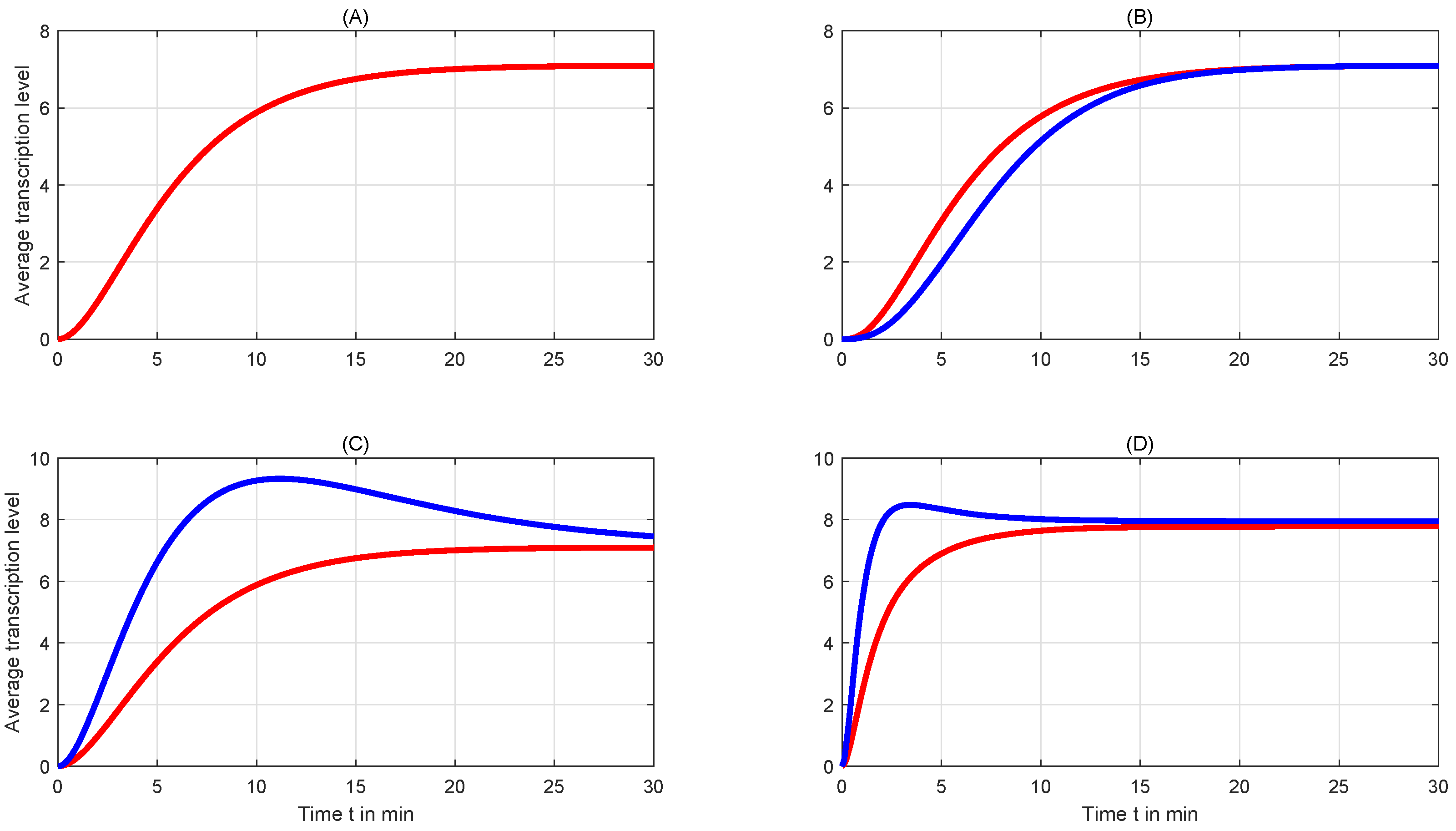
3.1. The Average Transcription Levels

In statistics, the expected value is a long-term average value of random variables. In this paper, it indicates the anticipated number of transcripts produced in single cells. It also indicates the probability-weighted average of all possible transcript numbers produced in a homologous genetic cell. In the following theorem, we give the analytical form of the average transcript level, which shows how many transcripts one expects to count per cell.

Theorem 1.

Assume that there are two activated states and one inactivated state; then, the average transcript level is given by

$$\begin{array}{cc}\hfill m\left(t\right)=& \frac{{\nu }_1\lambda {\gamma }_2+{\nu }_{2}p\lambda {\gamma }_1}{\alpha \beta \delta }-\frac{{\nu }_1\lambda ({\gamma }_2-\delta )+{\nu }_{2}p\lambda {\gamma }_1}{\delta (\alpha -\delta )(\beta -\delta )}{e}^{-\delta t}\hfill \\ \hfill & -\frac{{\nu }_1\lambda ({\gamma }_2-\alpha )+{\nu }_{2}p\lambda {\gamma }_1}{\alpha (\beta -\alpha )(\delta -\alpha )}{e}^{-\alpha t}-\frac{{\nu }_1\lambda ({\gamma }_2-\beta )+{\nu }_{2}p\lambda {\gamma }_1}{\beta (\alpha -\beta )(\delta -\beta )}{e}^{-\beta t},\hfill \end{array}$$

(22)

where $\alpha +\beta =\lambda +{\gamma }_1+{\gamma }_2,\alpha \beta =p\lambda {\gamma }_1+\lambda {\gamma }_2+q{\gamma }_1{\gamma }_2.$

When $\alpha =\delta$ or $\beta =\delta$, the level (22) is not well defined, but we can derive the mean $m\left(t\right)$ by taking the limits in (22) as $\alpha \to \delta$ or $\beta \to \delta$.

Proof. 

Since the two probabilities $P_{E_1}\left(t\right)$ and $P_{E_2}\left(t\right)$ have been derived, the average transcript level $m\left(t\right)$ can be obtained directly by solving (16) with the initial condition $m\left(0\right)=0$. To derive the second and the third moments, we need to calculate the exact forms of $m_1\left(t\right)$ and $m_2\left(t\right)$. Here, we use the Laplace transform to solve them. Multiplying (4)–(6) by m and summing the products leads to

$$\begin{array}{c}\hfill \left\{\begin{array}{c}{m}_0^{\prime }\left(t\right)=q{\gamma }_1{m}_1\left(t\right)-(\lambda +\delta )m_0\left(t\right),\hfill \\ m_1^{\prime }\left(t\right)={\nu }_1{P}_{E_1}\left(t\right)+\lambda m_0\left(t\right)+{\gamma }_2{m}_2\left(t\right)-({\gamma }_1+\delta )m_1\left(t\right),\hfill \\ m_2^{\prime }\left(t\right)={\nu }_2{P}_{E_2}\left(t\right)+p{\gamma }_1{m}_1\left(t\right)-({\gamma }_2+\delta )m_2\left(t\right).\hfill \end{array}\right.\end{array}$$

(23)

From the initial condition (8), we find that $m_0\left(0\right)=m_1\left(0\right)=m_2\left(0\right)=0$. Note that the analytical forms $P_{E_1}\left(t\right)$ and $P_{E_2}\left(t\right)$ have been given in Lemma 1. Thus, the differential system (23) is closed.

By applying the Laplace transform to the system (23), we obtain three algebraic equations, namely

$$\begin{array}{c}\hfill \left\{\begin{array}{c}s\mathcal{L}\left(m_0\right)=q{\gamma }_1\mathcal{L}\left(m_1\right)-(\lambda +\delta )\mathcal{L}\left(m_0\right),\hfill \\ s\mathcal{L}\left(m_1\right)={\nu }_1\mathcal{L}\left(P_{E_1}\right)+\lambda \mathcal{L}\left(m_0\right)+{\gamma }_2\mathcal{L}\left(m_2\right)-({\gamma }_1+\delta )\mathcal{L}\left(m_1\right),\hfill \\ s\mathcal{L}\left(m_2\right)={\nu }_2\mathcal{L}\left(P_{E_2}\right)+p{\gamma }_1\mathcal{L}\left(m_1\right)-({\gamma }_2+\delta )\mathcal{L}\left(m_2\right).\hfill \end{array}\right.\end{array}$$

Solving these algebraic equations and substituting (14), we derive

$$\begin{array}{c}\hfill \left\{\begin{array}{c}\mathcal{L}\left(m_0\right)=\frac{q{\nu }_1\lambda {\gamma }_1(s+{\gamma }_2)(s+\delta +{\gamma }_2)+pq{\nu }_2\lambda {\gamma }_1^2{\gamma }_2}{s(s+\alpha )(s+\beta )(s+\delta )(s+\delta +\alpha )(s+\delta +\beta )},\hfill \\ \mathcal{L}\left(m_1\right)=\frac{{\nu }_1\lambda (s+\delta +\lambda )(s+\delta +{\gamma }_2)(s+{\gamma }_2)+p{\nu }_2\lambda {\gamma }_1{\gamma }_2(s+\delta +\lambda )}{s(s+\alpha )(s+\beta )(s+\delta )(s+\delta +\alpha )(s+\delta +\beta )},\hfill \\ \mathcal{L}\left(m_2\right)=\frac{p\lambda {\gamma }_1\left[{\nu }_1(s+\delta +\lambda )(s+{\gamma }_2)+{\nu }_2[(s+\delta )(s+\delta +\lambda +{\gamma }_1)+p\lambda {\gamma }_1]\right]}{s(s+\alpha )(s+\beta )(s+\delta )(s+\delta +\alpha )(s+\delta +\beta )}.\hfill \end{array}\right.\end{array}$$

(24)

Then, applying the inverse Laplace transform to them, we obtain the exact forms of $m_0\left(t\right),m_1\left(t\right)$ and $m_2\left(t\right)$. For example, we rewrite $\mathcal{L}\left(m_0\right)$ as

$$\mathcal{L}\left(m_0\right)=\frac{A}{s}+\frac{B}{s+\alpha }+\frac{C}{s+\beta }+\frac{D}{s+\delta }+\frac{E}{s+\delta +\alpha }+\frac{F}{s+\delta +\beta }.$$

Then, reducing the above fraction to a common denominator gives

$$\begin{array}{cc}\hfill q{\nu }_1\lambda {\gamma }_1(s+{\gamma }_2)(s+\delta +{\gamma }_2)+pq{\nu }_2\lambda {\gamma }_1^2{\gamma }_2=& A(s+\alpha )(s+\beta )(s+\delta )(s+\delta +\alpha )(s+\delta +\beta )\hfill \\ \hfill & +\cdots +Fs(s+\alpha )(s+\beta )(s+\delta )(s+\delta +\alpha ).\hfill \end{array}$$

Let $s=0$, and we obtain

$$A=\frac{q{\nu }_1\lambda {\gamma }_1{\gamma }_2(\delta +{\gamma }_2)+pq{\nu }_2\lambda {\gamma }_1^2{\gamma }_2}{\alpha \beta \delta (\delta +\alpha )(\delta +\beta )}.$$

Then, let $s=-\alpha ,-\beta ,\cdots ,-\delta -\beta$, and we obtain $B,C,\cdots ,F$. Thus, $m_0\left(t\right)$ is given as

$$\begin{array}{cc}\hfill m_0\left(t\right)=& \frac{q{\nu }_1\lambda {\gamma }_1{\gamma }_2(\delta +{\gamma }_2)+pq{\nu }_2\lambda {\gamma }_1^2{\gamma }_2}{\alpha \beta \delta (\delta +\alpha )(\delta +\beta )}-\frac{q{\nu }_1\lambda {\gamma }_1{\gamma }_2({\gamma }_2-\delta )+pq{\nu }_2\lambda {\gamma }_1^2{\gamma }_2}{\delta (\alpha -\delta )(\beta -\delta )\alpha \beta }{e}^{-\delta t}\hfill \\ \hfill & -\frac{q{\nu }_1\lambda {\gamma }_1({\gamma }_2-\alpha )(\delta +{\gamma }_2-\alpha )+pq{\nu }_2\lambda {\gamma }_1^2{\gamma }_2}{\alpha (\beta -\alpha )(\delta -\alpha )\delta (\delta +\beta -\alpha )}{e}^{-\alpha t}\hfill \\ \hfill & -\frac{q{\nu }_1\lambda {\gamma }_1({\gamma }_2-\beta )(\delta +{\gamma }_2-\beta )+pq{\nu }_2\lambda {\gamma }_1^2{\gamma }_2}{\beta (\alpha -\beta )(\delta -\beta )(\delta +\alpha -\beta )\delta }{e}^{-\beta t}\hfill \\ \hfill & -\frac{q{\nu }_1\lambda {\gamma }_1({\gamma }_2-\alpha )({\gamma }_2-\delta -\alpha )+pq{\nu }_2\lambda {\gamma }_1^2{\gamma }_2}{(\delta +\alpha )\delta (\beta -\delta -\alpha )\alpha (\beta -\alpha )}{e}^{-(\delta +\alpha )t}\hfill \\ \hfill & -\frac{q{\nu }_1\lambda {\gamma }_1({\gamma }_2-\beta )({\gamma }_2-\delta -\beta )+pq{\nu }_2\lambda {\gamma }_1^2{\gamma }_2}{(\delta +\beta )(\alpha -\delta -\beta )\delta \beta (\alpha -\beta )}{e}^{-(\delta +\beta )t}.\hfill \end{array}$$

Similarly, we obtain exact forms of $m_1\left(t\right)$ and $m_2\left(t\right)$, which are

$$\begin{array}{cc}\hfill m_1\left(t\right)=& \frac{[{\nu }_1(\delta +{\gamma }_2)+p{\nu }_2{\gamma }_1]\lambda {\gamma }_2(\delta +\lambda )}{\alpha \beta \delta (\delta +\alpha )(\delta +\beta )}-\frac{[{\nu }_1({\gamma }_2-\delta )+p{\nu }_2{\gamma }_1]{\lambda }^2{\gamma }_2}{\delta (\alpha -\delta )(\beta -\delta )\alpha \beta }{e}^{-\delta t}\hfill \\ \hfill & -\frac{[{\nu }_1(\delta +{\gamma }_2-\alpha )({\gamma }_2-\alpha )+p{\nu }_2{\gamma }_1{\gamma }_2]\lambda (\delta +\lambda -\alpha )}{\alpha (\beta -\alpha )(\delta -\alpha )\delta (\delta +\beta -\alpha )}{e}^{-\alpha t}\hfill \\ \hfill & -\frac{[{\nu }_1(\delta +{\gamma }_2-\beta )({\gamma }_2-\beta )+p{\nu }_2{\gamma }_1{\gamma }_2]\lambda (\delta +\lambda -\beta )}{\beta (\alpha -\beta )(\delta -\beta )(\delta +\alpha -\beta )\delta }{e}^{-\beta t}\hfill \\ \hfill & -\frac{[{\nu }_1({\gamma }_2-\alpha )({\gamma }_2-\delta -\alpha )+p{\nu }_2{\gamma }_1{\gamma }_2]\lambda (\lambda -\alpha )}{(\delta +\alpha )\delta (-\beta -\delta -\alpha )\alpha (\beta -\alpha )}{e}^{-(\delta +\alpha )t}\hfill \\ \hfill & -\frac{[{\nu }_1({\gamma }_2-\beta )({\gamma }_2-\delta -\beta )+p{\nu }_2{\gamma }_1{\gamma }_2]\lambda (\lambda -\beta )}{(\delta +\beta )(\alpha -\delta -\beta )\delta \beta (\alpha -\beta )}{e}^{-(\delta +\beta )t},\hfill \\ \hfill m_2\left(t\right)=& \frac{\left[{\nu }_1(\delta +\lambda ){\gamma }_2+{\nu }_2[\delta (\delta +\lambda +{\gamma }_1)+p\lambda {\gamma }_1]\right]p\lambda {\gamma }_1}{\alpha \beta \delta (\delta +\alpha )(\delta +\beta )}-\frac{[{\nu }_1({\gamma }_2-\delta )+p{\nu }_2{\gamma }_1]p{\lambda }^2{\gamma }_1}{\delta (\alpha -\delta )(\beta -\delta )\alpha \beta }{e}^{-\delta t}\hfill \\ \hfill & -\frac{\left[{\nu }_1(\delta +\lambda -\alpha )({\gamma }_2-\alpha )+{\nu }_2[(\delta -\alpha )(\delta +\lambda +{\gamma }_1-\alpha )+p\lambda {\gamma }_1]\right]p\lambda {\gamma }_1}{\alpha (\beta -\alpha )(\delta -\alpha )\delta (\delta +\beta -\alpha )}{e}^{-\alpha t}\hfill \\ \hfill & -\frac{\left[{\nu }_1(\delta +\lambda -\beta )({\gamma }_2-\beta )+{\nu }_2[(\delta -\beta )(\delta +\lambda +{\gamma }_1-\beta )+p\lambda {\gamma }_1]\right]p\lambda {\gamma }_1}{\beta (\alpha -\beta )(\delta -\beta )(\delta +\alpha -\beta )\delta }{e}^{-\beta t}\hfill \\ \hfill & -\frac{\left[{\nu }_1(\lambda -\alpha )({\gamma }_2-\delta -\alpha )+{\nu }_2[p\lambda {\gamma }_1-\alpha (\lambda +{\gamma }_1-\alpha )]\right]p\lambda {\gamma }_1}{(\delta +\alpha )\delta (\beta -\delta -\alpha )\alpha (\beta -\alpha )}{e}^{-(\delta +\alpha )t}\hfill \\ \hfill & -\frac{\left[{\nu }_1(\lambda -\beta )({\gamma }_2-\delta -\beta )+{\nu }_2[p\lambda {\gamma }_1-\beta (\lambda +{\gamma }_1-\beta )]\right]p\lambda {\gamma }_1}{(\delta +\beta )(\alpha -\delta -\beta )\delta \beta (\alpha -\beta )}{e}^{-(\delta +\beta )t}.\hfill \end{array}$$

We rewrite them as

$$\begin{array}{c}\hfill m_0\left(t\right)=m_0^{*}+{\overline{m}}_0\left(t\right),m_1\left(t\right)=m_1^{*}+{\overline{m}}_1\left(t\right),m_2\left(t\right)=m_2^{*}+{\overline{m}}_2\left(t\right),\end{array}$$

(25)

for the sake of brevity, where ${\overline{m}}_0\left(t\right),{\overline{m}}_1\left(t\right),and{\overline{m}}_0\left(t\right)$ are damped exponentially and $m_0^{*}$$m_1^{*},m_2^{*}$ are given as

$$\begin{array}{cc}\hfill m_0^{*}=& \frac{q{\nu }_1\lambda {\gamma }_1{\gamma }_2(\delta +{\gamma }_2)+pq{\nu }_2\lambda {\gamma }_1^2{\gamma }_2}{\alpha \beta \delta (\delta +\alpha )(\delta +\beta )},\hfill \\ \hfill m_1^{*}=& \frac{[{\nu }_1(\delta +{\gamma }_2)+p{\nu }_2{\gamma }_1]\lambda {\gamma }_2(\delta +\lambda )}{\alpha \beta \delta (\delta +\alpha )(\delta +\beta )},\hfill \\ \hfill m_2^{*}=& \frac{\left[{\nu }_1(\delta +\lambda ){\gamma }_2+{\nu }_2[{\delta }^2+(\lambda +{\gamma }_1)\delta +p\lambda {\gamma }_1]\right]p\lambda {\gamma }_1}{\alpha \beta \delta (\delta +\alpha )(\delta +\beta )}.\hfill \end{array}$$

From (17), summing $m_0\left(t\right)$, $m_1\left(t\right)$, and $m_2\left(t\right)$ also gives the average transcript level $m\left(t\right)$. □

From (22), the level $m\left(t\right)$ has a limit when time t reaches infinity, i.e.,

$$\begin{array}{c}\hfill m^{*}=\underset{t\to \infty }{lim}m\left(t\right)=\frac{{\nu }_1\lambda {\gamma }_2+{\nu }_{2}p\lambda {\gamma }_1}{\delta (p\lambda {\gamma }_1+\lambda {\gamma }_2+q{\gamma }_1{\gamma }_2)}=\frac{{\nu }_1/{\gamma }_1+p{\nu }_2/{\gamma }_2}{p/\lambda +1/{\gamma }_1+q/{\gamma }_2}·\frac{1}{\delta }.\end{array}$$

The limitation implies that the stationary level can be characterized as

$$\begin{array}{c}\hfill \frac{\mathrm{Burst}\mathrm{size}\mathrm{in}1\mathrm{st}\mathrm{ON}+\mathrm{Burst}\mathrm{size}\mathrm{in}2\mathrm{nd}\mathrm{ON}}{\mathrm{Average}\mathrm{transcription}\mathrm{duration}}\times \mathrm{Average}\mathrm{lifetime}\mathrm{of}\mathrm{mRNAs}.\end{array}$$

Since the initial value of $m\left(t\right)$ is set to 0 and the gene resides in the OFF state, we wish to know the temporal profile of $m\left(t\right)$ thereafter. The following theorem gives a necessary and sufficient condition causing $m\left(t\right)$ to peak at some time point.

Theorem 2.

Assume that the three parameters $\alpha ,\beta$, and δ are real distinct numbers. If

$$\begin{array}{c}\hfill min\{\alpha ,\beta ,\delta \}>\frac{{\nu }_1{\gamma }_2+p{\nu }_2{\gamma }_1}{{\nu }_1}\end{array}$$

(26)

holds, then the mean level $m\left(t\right)$ peaks at some time ${\tau }_1$.

Proof. 

Differentiating $m\left(t\right)$ twice with respect to t gives

$$\begin{array}{cc}\hfill m^{\prime }\left(t\right)=& \frac{{\nu }_1\lambda ({\gamma }_2-\alpha )+{\nu }_{2}p\lambda {\gamma }_1}{(\beta -\alpha )(\delta -\alpha )}{e}^{-\alpha t}+\frac{{\nu }_1\lambda ({\gamma }_2-\beta )+{\nu }_{2}p\lambda {\gamma }_1}{(\alpha -\beta )(\delta -\beta )}{e}^{-\beta t}\hfill \\ \hfill & +\frac{{\nu }_1\lambda ({\gamma }_2-\delta )+{\nu }_{2}p\lambda {\gamma }_1}{(\alpha -\delta )(\beta -\delta )}{e}^{-\delta t},\hfill \\ \hfill m^{″}\left(t\right)=& -\frac{\alpha [{\nu }_1\lambda ({\gamma }_2-\alpha )+{\nu }_{2}p\lambda {\gamma }_1]}{(\beta -\alpha )(\delta -\alpha )}{e}^{-\alpha t}-\frac{\beta [{\nu }_1\lambda ({\gamma }_2-\beta )+{\nu }_{2}p\lambda {\gamma }_1]}{(\alpha -\beta )(\delta -\beta )}{e}^{-\beta t}\hfill \\ \hfill & -\frac{\delta [{\nu }_1\lambda ({\gamma }_2-\delta )+{\nu }_{2}p\lambda {\gamma }_1]}{(\alpha -\delta )(\beta -\delta )}{e}^{-\delta t}.\hfill \end{array}$$

At time $t=0$, we have $m^{\prime }\left(0\right)=0$ and $m^{″}\left(0\right)={\nu }_1\lambda$. Thus, $m\left(t\right)$ is increasing at $t=0$, and there exists a $T_1>0$ such that $m^{\prime }\left(t\right)>0$ for $t\in (0,T_1)$.

Since $\alpha ,\beta$ and $\delta$ are distinct, we assume that $\alpha <\beta <\delta$. Then, $m^{\prime }\left(t\right)$ can be rewritten as

$$m^{\prime }\left(t\right)=e^{-\delta t}·H\left(t\right),$$

where

$$\begin{array}{cc}\hfill H\left(t\right)=& \frac{{\nu }_1\lambda ({\gamma }_2-\alpha )+{\nu }_{2}p\lambda {\gamma }_1}{(\beta -\alpha )(\delta -\alpha )}{e}^{(\delta -\alpha )t}+\frac{{\nu }_1\lambda ({\gamma }_2-\beta )+{\nu }_{2}p\lambda {\gamma }_1}{(\alpha -\beta )(\delta -\beta )}{e}^{(\delta -\beta )t}\hfill \\ \hfill & +\frac{{\nu }_1\lambda ({\gamma }_2-\delta )+{\nu }_{2}p\lambda {\gamma }_1}{(\alpha -\delta )(\beta -\delta )}.\hfill \end{array}$$

Taking the limit as $t\to \infty$, we obtain

$$\underset{t\to \infty }{lim}H\left(t\right)=-\infty$$

when $\alpha >({\nu }_1{\gamma }_2+{\nu }_{2}p{\gamma }_1)/{\nu }_1$. Then, there exists a large $T_2>0$, such that $H\left(t\right)<0$ for all $t>T_2$. Taking these together, we find that there exists a unique ${\tau }_1\in (T_1,T_2)$ such that $m^{\prime }\left({\tau }_1\right)=0$. To prove the uniqueness, we only need to show that $H\left(t\right)$ has a unique critical point.

Differentiating $H\left(t\right)$ gives

$$H^{\prime }\left(t\right)=\frac{{\nu }_1\lambda ({\gamma }_2-\alpha )+{\nu }_{2}p\lambda {\gamma }_1}{\beta -\alpha }{e}^{(\delta -\alpha )t}+\frac{{\nu }_1\lambda ({\gamma }_2-\beta )+{\nu }_{2}p\lambda {\gamma }_1}{\alpha -\beta }{e}^{(\delta -\beta )t}.$$

Then, $H^{\prime }\left(t\right)=0$ has only one root over $(0,\infty )$. Combining $H\left(0\right)=0$ and $H^{\prime }\left(0\right)={\nu }_1\lambda >0$, we obtain that ${\tau }_1$ is unique. For other cases, we achieve the same conclusion by using similar discussions. □

We wish to determine when the condition (26) can be satisfied. Noticing that the degradation rate $\delta$ is independent of the five parameters in $({\nu }_1{\gamma }_2+{\nu }_{2}p{\gamma }_1)/{\nu }_1$ and $\beta >\alpha$ holds, we only need to guarantee $\alpha >({\nu }_1{\gamma }_2+{\nu }_{2}p{\gamma }_1)/{\nu }_1$. When ${\nu }_1\le {\nu }_2$ holds, we will show $\alpha <({\nu }_1{\gamma }_2+{\nu }_{2}p{\gamma }_1)/{\nu }_1$. We use the method of proof by contradiction. Suppose, on the contrary, that $\alpha \ge ({\nu }_1{\gamma }_2+{\nu }_{2}p{\gamma }_1)/{\nu }_1$. Then, $\lambda +{\gamma }_1>{\gamma }_2+2{\nu }_{2}p{\gamma }_1/{\nu }_1$ and

$${\left(\lambda +\frac{{\nu }_1-2p{\nu }_2}{{\nu }_1}{\gamma }_1-{\gamma }_2\right)}^2\ge {(\lambda +{\gamma }_1+{\gamma }_2)}^2-4(p\lambda {\gamma }_1+\lambda {\gamma }_2+q{\gamma }_1{\gamma }_2)$$

hold. It follows that

$$\lambda +{\gamma }_1\le \frac{(p{\nu }_2^2-{\nu }_1^2){\gamma }_1+({\nu }_1{\nu }_2-{\nu }_1^2){\gamma }_2}{{\nu }_1{\nu }_2-{\nu }_1^2}.$$

However, this contradicts $\lambda +{\gamma }_1>{\gamma }_2+2{\nu }_{2}p{\gamma }_1/{\nu }_1$. Thus, the inequality $\alpha \ge ({\nu }_1{\gamma }_2+{\nu }_{2}p{\gamma }_1)/{\nu }_1$ must be false. Therefore, $\alpha <({\nu }_1{\gamma }_2+{\nu }_{2}p{\gamma }_1)/{\nu }_1$.

When ${\nu }_1>{\nu }_2$ holds, $\alpha >({\nu }_1{\gamma }_2+{\nu }_{2}p{\gamma }_1)/{\nu }_1$ is equivalent to

$$({\nu }_1-{\nu }_2){\nu }_1(\lambda -{\gamma }_2)>({\nu }_1{\nu }_2-p{\nu }_2^2){\gamma }_1.$$

From the above analysis, we derive that, for a transcription system, the mean level $m\left(t\right)$ always exhibits increasing behavior if the mRNA molecules are stable. It is interesting to see that, only when mRNA molecules are easily degraded, the mean level $m\left(t\right)$ increases very abruptly and reaches its maximal value. It then decays and approaches its stationary value.

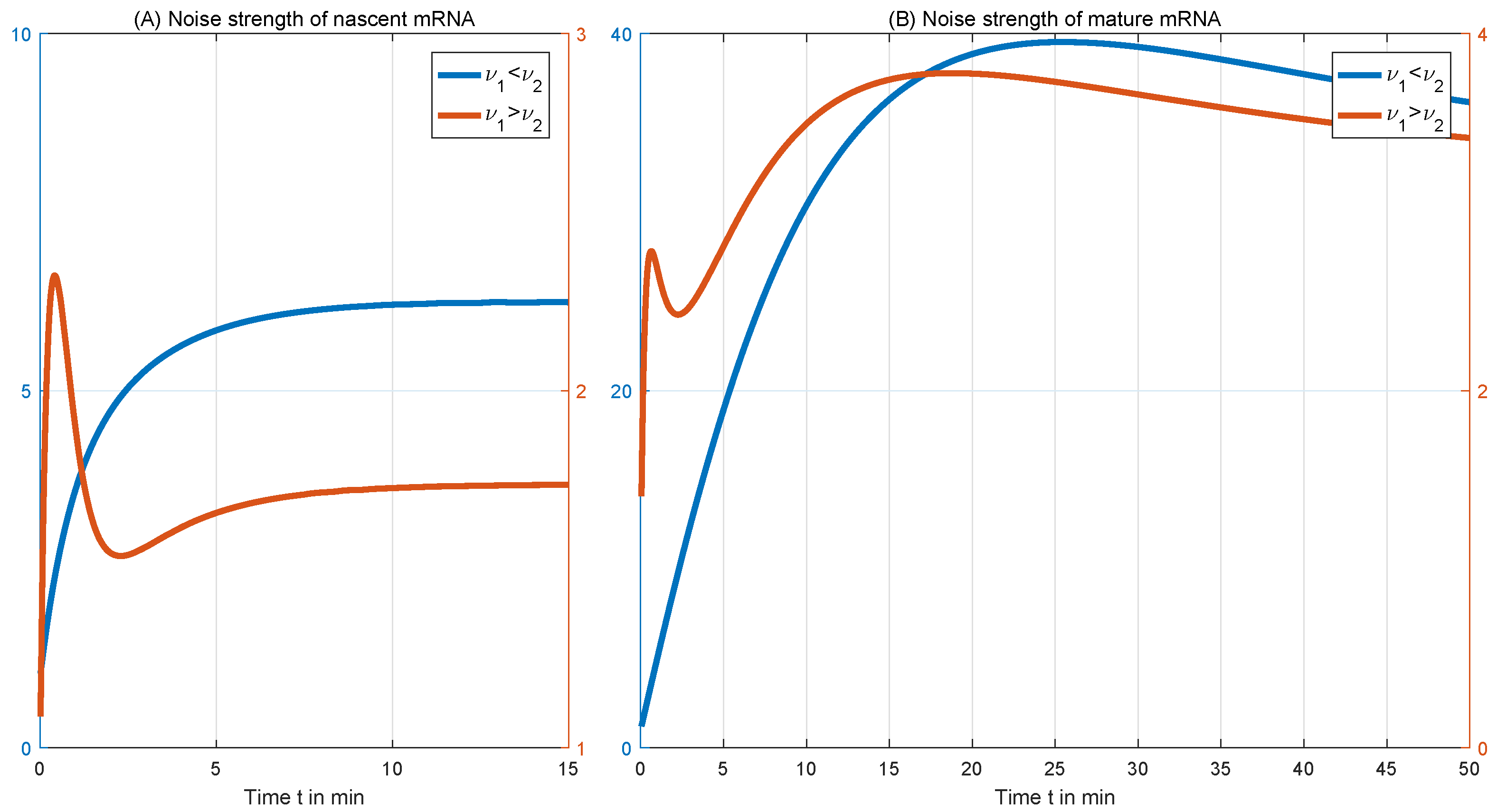
3.2. The Noise and the Skewness of Transcripts

In the past two decades, the noise ${\eta }^2\left(t\right)$ and the noise strength $\varphi \left(t\right)$ have been widely used to characterize the fluctuations of transcripts in cell populations. The noise is defined as the ratio between the variance and the mean square, and the noise strength is the ratio of the variance to the mean. Both of them are completely determined by the mean level $m\left(t\right)$ and the second moment $\mu \left(t\right)$. Thus, to derive the noise and the noise strength, we only need to calculate the second moment.

By definition, the second moment of transcripts is

$$\begin{array}{c}\hfill \mu \left(t\right)=\mathbf{E}\left[M^2\left(t\right)\right]=\sum _{m=0}^{\infty }{m}^2{P}_m\left(t\right).\end{array}$$

Multiplying (4)–(6) by $m^2$ and taking the sum, we derive (19) with the initial value $\mu \left(0\right)=0$. By solving the initial value problem, and we can obtain the exact form of $\mu \left(t\right)$.

Theorem 3.

Under the same condition of Theorem 1, the second moment $\mu \left(t\right)=\mathrm{E}\left[M^2\left(t\right)\right]$ of transcripts $M\left(t\right)$ takes the form

$$\begin{array}{c}\hfill \mu \left(t\right)={\mu }^{*}+\overline{\mu }\left(t\right),\end{array}$$

where the first coefficient is given by

$$\begin{array}{c}\hfill {\mu }^{*}=m^{*}+\frac{{\nu }_1^2\lambda {\gamma }_2(\delta +\lambda )(\delta +{\gamma }_2)+2{\nu }_1{\nu }_{2}p\lambda {\gamma }_1{\gamma }_2(\delta +\lambda )+{\nu }_2^{2}p\lambda {\gamma }_1({\delta }^2+\delta (\lambda +{\gamma }_1)+p\lambda {\gamma }_1)}{\alpha \beta {\delta }^2(\delta +\alpha )(\delta +\beta )},\end{array}$$

and $\overline{\mu }\left(t\right)$ is damped exponentially.

The second moment $\mu \left(t\right)$ approaches a stationary value ${\mu }^{*}$ when the time t reaches infinity. Then, the variance is determined by the mean $m^{*}$ and ${\mu }^{*}$, i.e.,

$$\begin{array}{cc}\hfill {\sigma }^{2*}=& {\mu }^{*}-{\left(m^{*}\right)}^2\hfill \\ \hfill =& m^{*}+{\left(m^{*}\right)}^2·\frac{\alpha \beta \delta -(\alpha +\beta )\delta \lambda -{\delta }^2\lambda }{\lambda (\delta +\alpha )(\delta +\beta )}+\frac{({\nu }_1^2{\gamma }_2+p{\nu }_2^2{\gamma }_1)(\delta +\lambda )+pq{\nu }_2^2{\gamma }_1^2\lambda }{\alpha \beta \delta (\delta +\alpha )(\alpha +\beta )}.\hfill \end{array}$$

and the stationary noise strength is

$$\begin{array}{c}\hfill {\varphi }^{*}=1+m^{*}·\frac{\alpha \beta \delta -(\alpha +\beta )\delta \lambda -{\delta }^2\lambda }{\lambda (\delta +\alpha )(\delta +\beta )}+\frac{({\nu }_1^2{\gamma }_2+p{\nu }_2^2{\gamma }_1)(\delta +\lambda )+pq{\nu }_2^2{\gamma }_1^2\lambda }{({\nu }_1\lambda {\gamma }_1+p{\nu }_2\lambda {\gamma }_1)(\delta +\alpha )(\alpha +\beta )},\end{array}$$

(27)

which is greater than 1.

Next, we provide the process by which to calculate the third moment of transcripts. Since the analytical form of the third moment is too long, we omit this expatiatory expression from the text. Multiplying (4)–(6) by $m^2$ and summing the products, we have

$$\begin{array}{c}\hfill \left\{\begin{array}{c}{\mu }_0^{\prime }\left(t\right)=\delta m_0\left(t\right)+q{\gamma }_1{\mu }_1\left(t\right)-(\lambda +2\delta ){\mu }_0\left(t\right),\hfill \\ {\mu }_1^{\prime }\left(t\right)={\nu }_1{P}_{E_1}\left(t\right)+(2{\nu }_1+\delta )m_1\left(t\right)+\lambda {\mu }_0\left(t\right)+{\gamma }_2{\mu }_2\left(t\right)-({\gamma }_1+2\delta ){\mu }_1\left(t\right),\hfill \\ {\mu }_2^{\prime }\left(t\right)={\nu }_2{P}_{E_2}\left(t\right)+(2{\nu }_2+\delta )m_2+p{\gamma }_1{\mu }_1\left(t\right)-({\gamma }_2+2\delta ){\mu }_2\left(t\right).\hfill \end{array}\right.\end{array}$$

(28)

From the initial condition (8), we find that ${\mu }_0\left(0\right)={\mu }_1\left(0\right)={\mu }_2\left(0\right)=0$. Note that the analytical forms $P_{E_1}\left(t\right)$ and $P_{E_2}\left(t\right)$ have been derived in Lemma 1, $m_0\left(t\right)$, $m_1\left(t\right)$ and $m_2\left(t\right)$ have been given in the proof of Theorem 1. Applying the Laplace transform to (28), we obtain

$$\begin{array}{c}\hfill \left\{\begin{array}{c}s\mathcal{L}\left({\mu }_0\right)=\delta \mathcal{L}\left(m_0\right)+q{\gamma }_1\mathcal{L}\left({\mu }_1\right)-(\lambda +2\delta )\mathcal{L}\left({\mu }_0\right),\hfill \\ s\mathcal{L}\left({\mu }_1\right)={\nu }_1\mathcal{L}\left(P_{E_1}\right)+(2{\nu }_1+\delta )\mathcal{L}\left(m_1\right)+\lambda \mathcal{L}\left({\mu }_0\right)+{\gamma }_2\mathcal{L}\left({\mu }_2\right)-({\gamma }_1+2\delta )\mathcal{L}\left({\mu }_1\right),\hfill \\ s\mathcal{L}\left({\mu }_2\right)={\nu }_2\mathcal{L}\left(P_{E_2}\right)+(2{\nu }_2+\delta )\mathcal{L}\left(m_2\right)+p{\gamma }_1\mathcal{L}\left({\mu }_1\right)-({\gamma }_2+2\delta )\mathcal{L}\left({\mu }_2\right).\hfill \end{array}\right.\end{array}$$

Solving these equations, we obtain the Laplace transforms of ${\mu }_0\left(t\right),{\mu }_1\left(t\right)$ and ${\mu }_2\left(t\right)$, which are linearly combined by $\mathcal{L}\left(P_{E_1}\right),\mathcal{L}\left(P_{E_2}\right)$ and $\mathcal{L}\left(m_0\right),\mathcal{L}\left(m_1\right),\mathcal{L}\left(m_2\right)$. Then, substituting (14) and (24) into the above equations gives $\mathcal{L}\left({\mu }_0\right),\mathcal{L}\left({\mu }_1\right)$ and $\mathcal{L}\left({\mu }_2\right)$.

Next, we use the Laplace transform (21) and obtain

$$\begin{array}{cc}\hfill \mathcal{L}\left(k_3\right)=& {\nu }_1[\mathcal{L}\left(P_{E_1}\right)+3\mathcal{L}\left(m_1\right)+3\mathcal{L}\left({\mu }_1\right)]+{\nu }_2[\mathcal{L}\left(P_{E_2}\right)+3\mathcal{L}\left(m_2\right)+3\mathcal{L}\left({\mu }_2\right)]\hfill \\ \hfill & -\delta [\mathcal{L}\left(m\right)-3\mathcal{L}\left(\mu \right)+3\mathcal{L}\left(k_3\right)],\hfill \end{array}$$

which can be rewritten as

$$\begin{array}{c}\hfill \mathcal{L}\left(k_3\right)=\frac{{\nu }_1[\mathcal{L}\left(P_{E_1}\right)+3\mathcal{L}\left(m_1\right)+3\mathcal{L}\left({\mu }_1\right)]+{\nu }_2[\mathcal{L}\left(P_{E_2}\right)+3\mathcal{L}\left(m_2\right)+3\mathcal{L}\left({\mu }_2\right)]+\delta [3\mathcal{L}\left(\mu \right)-\mathcal{L}\left(m\right)]}{s+3\delta }.\end{array}$$

Substituting (14), (24), $\mathcal{L}\left({\mu }_1\right)$, and $\mathcal{L}\left({\mu }_2\right)$ into the above equation, we obtain a fraction with respect to s. It is easy to solve the algebraic equation and convert the transformed function back into the original function. This function $k_3\left(t\right)$ is the third moment of transcripts. Let $k_3^{*}$ be the limit of $k_3\left(t\right)$. By the definition, we obtain the analytical form of the skewness, which takes the form

$$\begin{array}{c}\hfill S\left(t\right)=S^{*}+\overline{S}\left(t\right),\end{array}$$

where $\overline{S}\left(t\right)$ decays exponentially, and

$$S^{*}=\frac{k_3^{*}-3{\mu }^{*}{m}^{*}+2{\left(m^{*}\right)}^3}{{\left({\sigma }^{*}\right)}^3}.$$

4. Simulation and Discussion

With the development of detection techniques, such as single-molecule fluorescence in situ hybridization (smFISH) [25] and the single-cell RNA sequencing method (scRNA-seq) [26], huge amounts of experimental data are obtained through the real-time monitoring of transcription in individual living cells. These data have been applied to reveal random gene expression, identify gene regulatory mechanisms, and investigate the dynamics of physiological processes. In the following, we use numerical simulations to demonstrate the predictions achievable with our model. Data were analyzed and numerical simulations were performed using Matlab 9.4.0.813654 (R2018a https://ww2.mathworks.cn, accessed on 4 March 2022) [27].

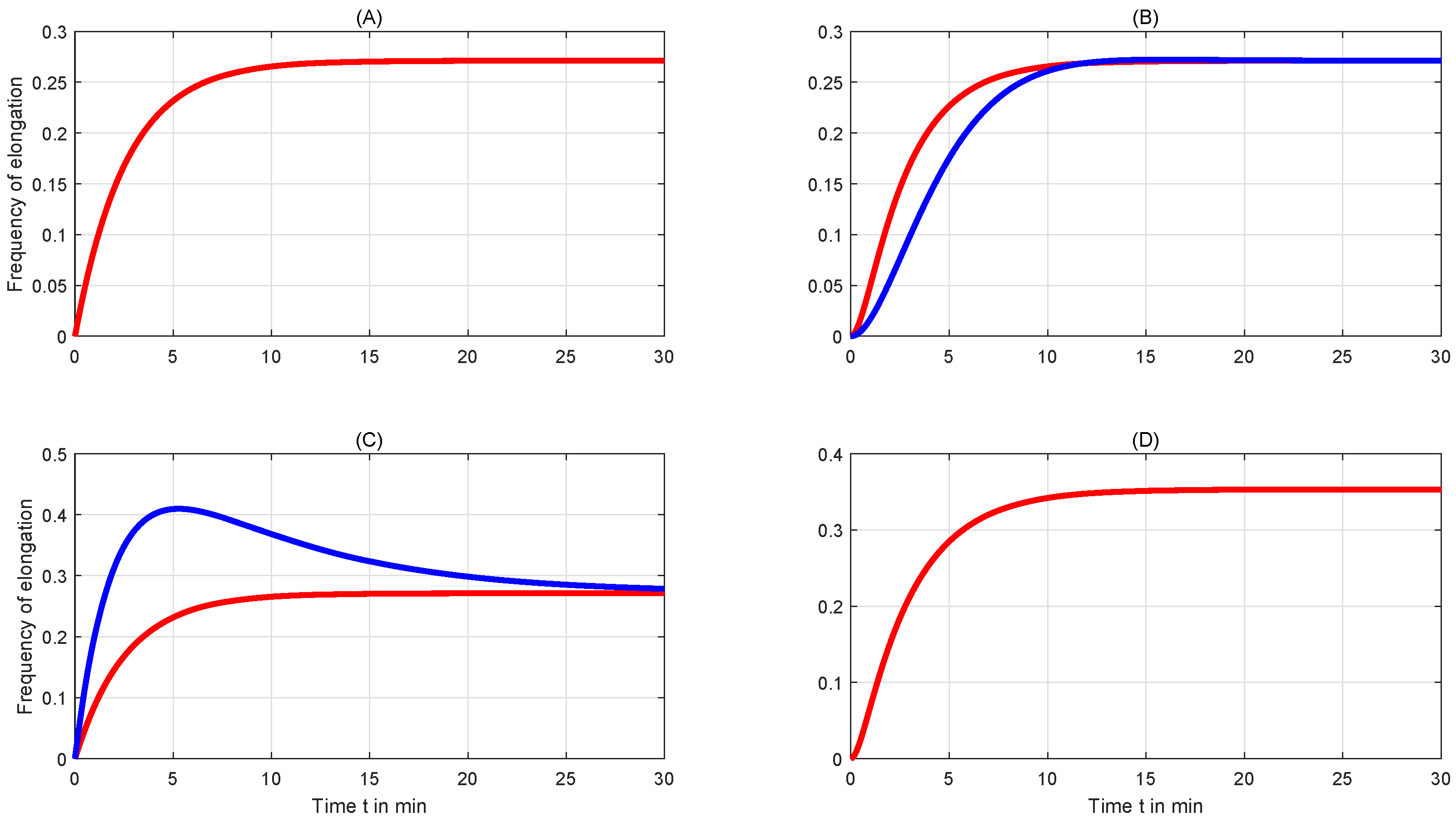
4.1. Comparison of Frequencies in Different Transcription Systems

By definition, the frequency $P_E\left(t\right)$ can be used to depict the ratio of cells that the target genes are transcribing as mRNA molecules. The real-time value of $P_E\left(t\right)$ can be derived by monitoring fluorescent proteins, and its dynamics have been widely discussed [9,28].

In the two-state transcription system, the promoter switches randomly between active and inactive states. The dynamics of frequency are very simple, increasing continuously and approaching a stationary value, as shown in Figure 2A. When there are two OFF states, the system transfers between the two OFF states and the ON state, and the frequency has two modes, as shown in Figure 2B: one is increasing and approaching its limit value (red curve), while the other one is an oscillatory function (blue curve). Since it is damped by the exponential function, the oscillation in the frequency of elongation may not be easily observed in experiments. The transcription regulated by cross-talking pathways was firstly established in 2012 [28]. In this system, the frequency also has two modes, as shown in Figure 2C. One mode shows that the frequency increases from 0 to approach its stationary value (red curve), and the other one is that the frequency may reach its stationary value in a limited time and remain above this level thereafter (blue curve). This means that cross-talking signaling pathways are capable of inducing more cells to transcribe than the steady-state level after a short time period of signal transduction. The two-ON-state transcription system established here has only one mode; that is, the frequency is increasing continuously and approaching its stationary value, as shown in Figure 2D.

By the above comparison, when the frequency exhibits a simple behavior, as shown by the red curves, it is difficult to distinguish which system is used to transcribe mRNA molecules. Only when a more complex behavior exists, such as shown by the blue curves in (C) and (D), can we eliminate some impossible systems. To confirm the transcription mechanism, we need more information from experimental data. In the next subsection, we compare the mean levels to further analyze the system that will be used.

4.2. Comparison of Mean Levels

From the real-time monitoring of transcription in individual living cells, we could obtain the average nascent/mature mRNA levels at different time points. In Theorem 1, we have given the dynamical expression of the average mRNA level for the transcription model that is established in Section 2. By comparing the analytical form with the observed data, we could confirm or rule out the established model.

In Figure 3, we compare the dynamical behaviors of average mRNA levels produced in different systems. As shown in Figure 3A, the average mRNA levels produced in the two-state transcription model increase over $(0,\infty )$ and approach their stationary values. In the three-state transcription model, the average mRNA levels exhibit two different behaviors: one is increasing monotonically—see the red curve in Figure 3B—and the other is damped oscillating—see the blue curve in Figure 3B—which may not be easily observed in experiments. For the situation wherein the transcription is activated by two competitive pathways, Sun et al. [29] gave a necessary and sufficient condition for the existence of the expression peak value; see Figure 3C. For the two-ON transcription model that we have established in this paper, the average mRNA levels also exhibit two behaviors; see Figure 3D. We also give a necessary and sufficient condition for the existence of the expression peak value. The expression peak occurs only when the mRNA is easily degraded, and the synthesis rate is larger in the first ON state.

From Figure 3, we find that the average mRNA levels produced by the cross-talking pathway activated transcription system and the two-ON transcription system are similar. More properties of the levels produced by the cross-talking pathway activated transcription system can be found in [12,30].

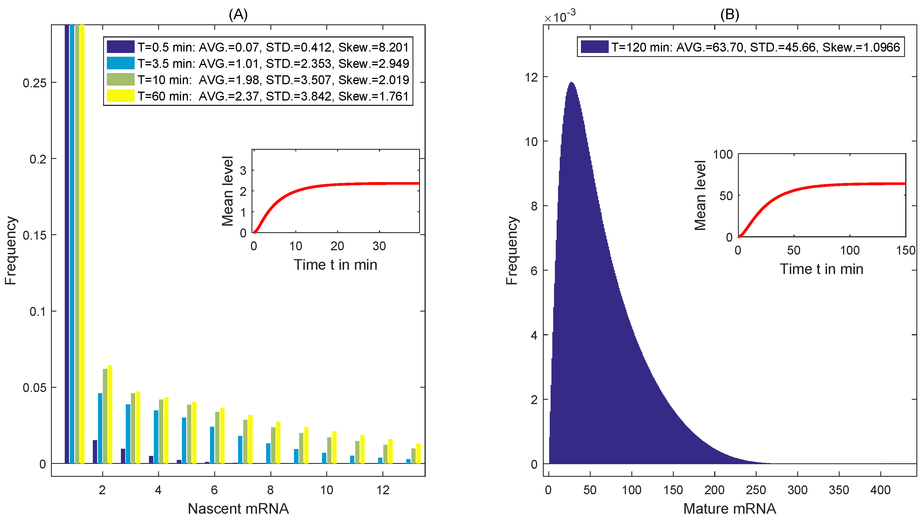
4.3. The Distribution of Transcripts

Usually, the mass probability function $P_m$ is difficult to calculate. Only under some special cases can it be derived [12,31]. In this subsection, we use the experimental data to simulate the distribution of transcripts produced in the two-ON transcription system. Using the smFISH approach, Senecal et al. [6] measured c-Fos transcription and derived the c-Fos mature and nascent mRNA numbers in individual cells. The data that we collated are as follows:

$$\begin{array}{c}\hfill \begin{array}{c}{T}_{Off}=9.24\min ,T_{On1}=1.916\min ,T_{On2}=4.23\min ,\\ {\delta }_{Nascent}=1.25{\min }^{-1},{\delta }_{Mature}=0.0462{\min }^{-1},\\ {\nu }_{On1}=6.16{\min }^{-1},{\nu }_{On2}=13.6{\min }^{-1},p=0.293,q=0.707.\end{array}\end{array}$$

(29)

The average durations for which the promoter resides at the OFF and the two ON states follow exponential distributions with rates $0.1082,0.5219$ and $0.2364$, respectively. The probability that the system leaves the first ON state and enters the second ON state is $0.293$. Then, the transfer rate from the first ON state to the second ON state is $0.1529$, and the rate from the first ON state to the OFF state is $0.3690$. The synthesis rates are $6.16$ during the first ON state and $13.6$ in the second ON state. The degradation rate for mature mRNA is set at $0.0462$ min${}^{-1}$; thus, the half-life is approximately 15 min [6,32]. In our simulation, the nascent mRNAs are assumed to degrade as a first-order reaction with a constant ${\delta }_{Nascent}=1.25$ min${}^{-1}$, and then the condition (26) holds.

Utilizing a modified finite-state projections analysis [33], we derived the distribution of mRNA molecules at different time points; see Figure 4 for details. When ${\nu }_1<{\nu }_2$, the nascent mRNA molecules exhibit a decaying distribution; that is, $P_m\left(t\right)$ is decreasing in m. When the time t takes a large value, the skewness is small, causing the distribution to display a long distribution tail; see Figure 4A. For mature mRNAs, the distribution exhibits a unimodal distribution when time t is large. The skewness is positive, meaning that the distribution has a long right tail.

To make condition (26) hold, we exchange the synthesis rates in the two ON states and accelerate the active rate in the OFF state. The data are given as

$$\begin{array}{c}\hfill \begin{array}{c}{T}_{Off}=0.33\min ,T_{On1}=1.916\min ,T_{On2}=4.23\min ,\\ {\delta }_{Nascent}=1.25{\min }^{-1},{\delta }_{Mature}=0.0462{\min }^{-1},\\ {\nu }_{On1}=13.6{\min }^{-1},{\nu }_{On2}=6.16{\min }^{-1},p=0.293,q=0.707.\end{array}\end{array}$$

(30)

For the nascent mRNA molecules, the insert in Figure 5A shows the temporal profile of the nascent mRNA level. The average mRNA level peaks at $t=3.5$ min and then decreases slowly. Compared with the profile of the mature mRNA level, the peak in mRNA levels occurs only when the half-life of transcripts is short, and the DNA duplex is easily opened to form a transcription bubble. This conclusion has also been proven in the competing pathway transcription system [29]. The histogram shows that the distribution changes from a decaying distribution to a bimodal distribution and then to a unimodal distribution at different time points. The skewness of distributions is positive, implying that all four distributions have a right distribution tail. By calculation, we find that the distribution has the smallest positive skewness at the moment that the transcript expression peaks. At steady state, the mean mRNA level and the skewness finally level out at around 8 and $0.445$.

For the mature mRNA molecules, the skewness is negative, which means that the distribution right tail has been shortened and the transcript numbers in single cells are mainly distributed around the mean value. In addition, we also find when the half-life of mRNAs increases, the skewness will be reduced further.

After serum induction, mature mRNA numbers at different time points were determined by using single-molecule FISH to quantify c-Fos transcription [6]. The numbers show that the mature mRNA levels decreased rapidly and returned to basal expression after reaching a maximum. Our model cannot simulate such a quick reduction, but it simulates the expression of the phosphorylated kinases ERK1/2 well. The diversity between the two expressions may be caused by different transcription mechanisms [4,21]:

We show the temporal profiles of noise strength in Figure 6. Similar to the average mRNA level, the behavior of the noise strength of both nascent and mature RNA is simple when the synthesis rate ${\nu }_2$ is greater, as shown by the blue curves in Figure 6. If the synthesis rate ${\nu }_1$ is greater, the noise strength exhibits a more complex behavior, as shown by the red curves.

5. Conclusions

Transcription kinetics are highly gene-specific [4,21]. To confirm the corresponding regulation mechanisms used by genes during transcription, many experimental techniques [34,35] and theoretical models with multiple stages [36,37] or in non-Markovian biochemical reaction systems [16,38] have been established during the last three decades. Using smFISH, Senecal et al. [6] detected up to four active c-Fos transcription sites per cell. Temporal variation in the number of active sites results in the switching of different initiation rates during elongation. By assuming that there are two active states and one inactive state of the promoter switching randomly to produce mRNA chains, we established a transcription model. Using this model, we studied the temporal behavior of transcription and its corresponding mechanism.

We derived the exact forms of the average transcript level and the noise strength, and then proved that this level may peak only when the transcripts are unstable, the synthesis rate in the first active state is higher and the DNA chain is easily unwound to form a stable preinitiation complex. We compared the behaviors of the elongation frequencies and the average transcript levels with those of three other transcription systems. If the transcription of a gene obeys the model described in Figure 1, the elongation frequency shows a simple behavior, which is increasing. The average level may increase continually or peak at some time point. Through these comparisons, we can reject some impractical models.

We also calculated the noise strength to characterize the fluctuation in the mRNA numbers, which shows a complex behavior when the synthesis rate in the first ON state is greater than that in the second one. To better depict the distribution of transcripts, we provided an effective method to calculate the skewness. For a further analysis, we will confirm all parameters related to transcription systems from experimental data with the help of appropriate algorithms [33,39,40] and parameter estimations [41,42]. These data help us to simulate and analyze behaviors of transcription. When the synthesis rate of the second active state is greater than that of the first one, the skewness is always positive, and the distribution of transcripts is skewed to the right, which is in agreement with published results [6]. However, the average mRNA level is increasing, and it cannot peak at some time point. We modified some experimental data and simulated transcription again. When the system has a higher synthesis rate in the first ON state, the distribution of transcripts is also right-skewed when the degradation rate is large. We found that, when the degradation rate decreases, the skewness also decreases. When the half-life of transcripts is large enough, the distribution could change to be left-skewed and has a fatter left tail. Our simulations can match some mRNA numbers and distributions well, especially for nascent mRNA. However, for other genes, there is a gap between our simulations and observed data of mature mRNA. The basic reason for this is that the intrinsic regulation mechanism remains unknown, which motivates us to make a further attempt in the future.

An enhancer could affect transcription through enhancer–promoter interactions, which depend on its contact probability with the promoter [7]. Enhancer contacts modulate burst frequency [7] or transcription initiation [43]. Variations in the enhancer number and their distances to the promoter cause the contacts to vary at discrete times, resulting in variation in the initiation rates. Our results give a potential method with which to study the contact probability and to explore the linear or nonlinear relationships among the enhancer, promoter, and initiation rate.

References

1. Elowitz, M.B.; Levine, A.J.; Siggia, E.D.; Swain, P.S. Stochastic gene expression in a single cell. Science 2002, 297, 1183. [Google Scholar] [CrossRef] [PubMed] [Green Version]
2. Golding, I.; Paulsson, J.; Zawilski, S.M.; Cox, E.C. Real-time kinetics of gene activity in individual bacteria. Cell 2005, 123, 1025. [Google Scholar] [CrossRef] [Green Version]
3. Blake, W.J.; Kaern, M.; Cantor, C.R.; Collins, J.J. Noise in eukaryotic gene expression. Nature 2003, 422, 633. [Google Scholar] [CrossRef] [PubMed]
4. Suter, D.M.; Molina, M.; Gatfield, D.; Schneider, K.; Schibler, U.; Naef, F. Mammalian genes are transcribed with widely different bursting kinetics. Science 2011, 332, 472. [Google Scholar] [CrossRef] [PubMed] [Green Version]
5. Bartman, C.R.; Hamagami, N.; Keller, C.A.; Giardine, B.; Hardison, R.C.; Blobel, G.A.; Raj, A. Transcriptional burst initiation and polymerase pause release are key control points of transcriptional regulation. Mol. Cell 2019, 79, 519. [Google Scholar] [CrossRef] [PubMed] [Green Version]
6. Senecal, A.; Munsky, B.; Proux, F.; Ly, N.; Braye, F.E.; Zimmer, C.; Mueller, F.; Darzacq, X. Transcription factors modulate c-Fos transcriptional bursts. Cell Rep. 2014, 8, 75–83. [Google Scholar] [CrossRef] [PubMed]
7. Zuin, J.; Roth, G.; Zhan, Y.; Cramard, J.; Redolfi, J.; Piskadlo, E.; Mach, P.; Kryzhanovska, M.; Tihanyi, G.; Kohler, H.; et al. Nonlinear control of transcription through enhancer-promoter interactions. Nature 2022, 604, 571–577. [Google Scholar] [CrossRef] [PubMed]
8. Peccoud, J.; Ycart, B. Markovian modeling of gene-product synthesis. Theor. Popul. Biol. 1995, 48, 222. [Google Scholar] [CrossRef]
9. Tang, M. The mean and noise of stochastic gene transcription. J. Theor. Biol. 2008, 253, 271–280. [Google Scholar] [CrossRef]
10. Cao, Z.; Filatova, T.; Oyarzun, D.A.; Grima, R. A stochastic model of gene expression with polymerase recruitment and pause release. Biophys. J. 2020, 119, 1002–1014. [Google Scholar] [CrossRef]
11. Sun, Q.; Cai, Z.; Zhu, C. A novel dynamical regulation of mRNA distribution by cross-talking pathways. Mathematics 2022, 10, 1515. [Google Scholar] [CrossRef]
12. Zhu, C.; Han, G.; Jiao, F. Dynamical regulation of mRNA distribution by cross-talking signaling pathways. Complexity 2020, 2020, 6402703. [Google Scholar] [CrossRef]
13. Chen, J.; Jiao, F. A novel approach for calculating exact forms of mRNA distribution in single-cell measurements. Mathematics 2022, 10, 27. [Google Scholar] [CrossRef]
14. Cao, Z.; Grima, R. Analytical distributions for detailed models of stochastic gene expression in eukaryotic cells. Proc. Natl. Acad. Sci. USA 2020, 117, 4682–4692. [Google Scholar] [CrossRef] [Green Version]
15. Jia, C.; Grima, R. Frequency domain analysis of fluctuations of mRNA and protein copy numbers within a cell lineage: Theory and experimental validation. Phys. Rev. X 2021, 11, 021032. [Google Scholar] [CrossRef]
16. Zhang, J.; Zhou, T. Markovian approaches to modeling intracellular reaction processes with molecular memory. Proc. Natl. Acad. Sci. USA 2019, 116, 23542–23550. [Google Scholar] [CrossRef] [Green Version]
17. Zopf, C.J.; Quinn, K.; Zeidman, J.; Maheshri, N. Cell-cycle dependence of transcription dominates noise in gene expression. PLoS Comput. Biol. 2013, 9, e1003161. [Google Scholar] [CrossRef] [Green Version]
18. Sun, Q.; Jiao, F.; Lin, G.; Yu, J.; Tang, M. The nonlinear dynamics and fluctuations of mRNA levels in cell cycle coupled transcription. PLoS Comput. Biol. 2019, 15, e100701. [Google Scholar] [CrossRef]
19. Jiao, F.; Tang, M. Quantification of transcription noise’s impact on cell fate commitment with digital resolutions. Bioinformatics 2022, 38, 3062–3069. [Google Scholar] [CrossRef]
20. Sun, Q.; Jiao, F.; Yu, J. The dynamics of gene transcription with a periodic synthesis rate. Nonlinear Dynamcis 2021, 104, 4477–4492. [Google Scholar] [CrossRef]
21. Larson, D.R. What do expression dynamics tell us about the mechanism of transcription? Curr. Opin. Genet. Dev 2011, 21, 591–599. [Google Scholar] [CrossRef] [PubMed] [Green Version]
22. Huang, L.; Yuan, Z.; Liu, P.; Zhou, T. Effects of promoter leakage on dynamics of gene expression. BMC Syst. Biol. 2015, 9, 16. [Google Scholar] [CrossRef] [PubMed] [Green Version]
23. Smith, S.; Grima, R. Plasticity of the truth table of low-leakage genetic logic gates. Phys. Rev. E 2018, 98, 062410. [Google Scholar] [CrossRef] [Green Version]
24. Weisstein, E.W. Laplace Transform. Available online: https://mathworld.wolfram.com/ (accessed on 8 August 2020).
25. Raj, A.; van den Bogaard, P.; Rifkin, S.A.; van Oudenaarden, A.; Tyagi, S. Imaging individual mRNA molecules using multiple singly labeled probes. Nat. Methods 2008, 5, 877–879. [Google Scholar] [CrossRef] [Green Version]
26. Tang, F.; Barbacioru, C.; Wang, Y.; Nordman, E.; Lee, C.; Xu, N.; Wang, X.; Bodeau, J.; Tuch, B.B.; Siddiqui, A.; et al. mRNA-Seq wholetranscriptome analysis of a single cell. Nat. Methods 2009, 6, 377–382. [Google Scholar] [CrossRef]
27. MathWorks. Matlab 9.4.0.813654 (R2018a). Available online: https://ww2.mathworks.cn (accessed on 4 March 2020).
28. Sun, Q.; Tang, M.; Yu, J. Temporal profile of gene transcription noise modulated by cross-talking signal transduction pathways. Bull. Math. Biol. 2012, 74, 375–398. [Google Scholar] [CrossRef]
29. Yu, J.; Sun, Q.; Tang, M. The nonlinear dynamics and fluctuations of mRNA levels in cross-talking pathway activated transcription. J. Theor. Biol. 2014, 363, 223–234. [Google Scholar] [CrossRef]
30. Jiao, F.; Zhu, C. Regulation of gene activation by competitive cross talking pathways. Biphysical J. 2020, 119, 1204–1214. [Google Scholar] [CrossRef]
31. Jiao, F.; Ren, J.; Yu, J. Analytical formula and dynamic profile of mRNA distribution. Discret. Contin. Dyn. Syst. B 2020, 25, 241–257. [Google Scholar] [CrossRef] [Green Version]
32. Shyu, A.B.; Greenberg, M.E.; Belasco, J.G. The c-Fos transcript is targeted for rapid decay by two distinct mRNA degradation pathways. Genes Dev. 1989, 3, 60–72. [Google Scholar] [CrossRef] [Green Version]
33. Munsky, B.; Khammash, M. The finite state projection algorithm for the solution of the chemical master equation. J. Chem. Phys. 2006, 124, 044104. [Google Scholar] [CrossRef] [PubMed]
34. Müller, G.A.; Stangner, K.; Schmitt, T.; Wintsche, A.; Engeland, K. Timing of transcription during the cell cycle: Protein complexes binding to E2F, E2F/CLE, CDE/CHR, or CHR promoter elements define early and late cell cycle gene expression. Oncotarget 2017, 8, 97736–97748. [Google Scholar] [CrossRef] [Green Version]
35. Caveney, P.M.; Norred, S.E.; Chin, C.W.; Boreyko, J.B.; Razooky, B.S.; Retterer, S.T.; Collier, C.P.; Simpson, M.L. Resource sharing controls gene expression bursting. ACS Synth. Biol. 2017, 6, 334–343. [Google Scholar] [CrossRef] [PubMed]
36. Jia, C. Simplification of Markov chains with infinite state space and the mathematical theory of random gene expression bursts. Phys. Rev. E 2017, 96, 032402. [Google Scholar] [CrossRef] [PubMed] [Green Version]
37. Jia, C. Kinetic foundation of the zero-inflated negative binomial model for single-cell RNA sequencing data. SIAM J. Appl. Math. 2020, 80, 1336–1355. [Google Scholar] [CrossRef]
38. Yang, X.; Chen, Y.; Zhou, T.; Zhang, J. Exploring dissipative sources of non-Markovian biochemical reaction systems. Phys. Rev. E 2021, 103, 052411. [Google Scholar] [CrossRef] [PubMed]
39. Peng, J.; Kocarev, L. First encounters on Bethe lattices and Cayley trees. Commun. Nonlinear Sci. Numer. Simul. 2021, 95, 105594. [Google Scholar] [CrossRef]
40. Gao, L.; Peng, J.; Tang, C. Optimizing the first-passage process on a class of fractal scale-free trees. Fractal Fract. 2021, 5, 184. [Google Scholar] [CrossRef]
41. Chen, L.; Zhu, C.; Jiao, F. A generalized moment-based method for estimating parameters of stochastic gene transcription. Math. Biosci. 2022, 345, 108780. [Google Scholar] [CrossRef]
42. Cao, Z.; Grima, R. Accuracy of parameter estimation for auto-regulatory transcriptional feedback loops from noisy data. J. R. Soc. Interface 2019, 16, 20180967. [Google Scholar] [CrossRef]
43. Larke, M.S.C.; Schwessinger, R.; Nojima, T.; Telenius, J.; Beagrie, R.A.; Downes, D.J.; Oudelaar, A.M.; Truch, J.; Graham, B.; Bender, M.A.; et al. Enhancers predominantly regulate gene expression during differentiation via transcription initiation. Mol. Cell 2021, 81, 983–997.e7. [Google Scholar] [CrossRef] [PubMed]
Figure 1. The stochastic transition of transcription with two active states and one inactive state.
Mathematics 10 02189 g001
Figure 2. The temporal profiles of elongation frequency in different transcription systems; (A) two-state transcription system; (B) three-state transcription system; (C) the cross-talking transcription system; (D) two-ON transcription system.
Mathematics 10 02189 g002
Figure 3. The mean transcription levels produced in different systems. (A) two-state transcription system; (B) three-state transcription system; (C) the cross-talking transcription system; (D) two-ON transcription system.
Mathematics 10 02189 g003
Figure 4. (A) The distribution of nascent mRNAs when ν 1 < ν 2 at different times; (B) the distribution of mature mRNAs when ν 1 < ν 2 at T = 120 min. Parameters are given in (29).
Mathematics 10 02189 g004
Figure 5. (A) The distribution of nascent mRNAs when ν 1 > ν 2 at different times; (B) the distribution of mature mRNAs when ν 1 > ν 2 at T = 120 min. Parameters are given in (30).
Mathematics 10 02189 g005
Figure 6. (A) Noise strengths of nascent mRNAs for cases ν 1 < ν 2 and ν 1 > ν 2 ; (B) noise strengths of mature mRNAs for cases ν 1 < ν 2 and ν 1 > ν 2 .
Mathematics 10 02189 g006
Publisher’s Note: MDPI stays neutral with regard to jurisdictional claims in published maps and institutional affiliations.