Predicting the Business Cycle in South Africa: Insights from a Real-Financial Activity Gap

Abstract

Traditional approaches to predicting business cycles are limited by their omission of financial variables, which, in turn, leads to failures to signal financial-sector crises and to misestimate the duration and intensity of economic events. This study addresses this challenge by constructing a real-financial activity gap for South Africa and utilising it to predict the occurrence of economic recoveries. The study examines the period from 1970Q1 to 2023Q4, using real GDP, domestic credit, house prices, and share prices. The dynamic factor model and the Hodrick–Prescott filter are employed to construct the real-financial activity gap. The recursive ADF unit root test is used to assess the presence, frequency, and duration of economic recoveries. To validate the results, a Markov switching dynamic regression model is applied. The results reveal that the new gap tends to produce economic recovery predictions that are less frequent but longer in duration. In contrast, predictions based on real GDP lead to more frequent but shorter recoveries. The new gap suggests that financial variables contribute to stabilising growth over extended periods, whereas real GDP reflects quicker but more volatile economic adjustments. The latest gap offers a more stable basis for forecasting recoveries, aiding policymakers in better anticipating and mitigating economic downturns. Accordingly, the output gap and the real-financial activity gap should be used as complements.

1. Introduction

The experience of the global financial crisis in 2007/09 challenged existing business cycle models and necessitated the incorporation of financial variables in business cycle models. Existing business cycle models, such as the real business cycle model (RBC) and the new Keynesian model (NKM), ignored the role of financial variables in instigating and propagating macroeconomic developments, and, as a result, they were unable foresee the financial vulnerabilities that crept up over time and ultimately led to the devasting crisis in 2007/09 (Adarov, 2021, 2023). Against this backdrop, there have been increasing efforts to examine financial variables closely. Earlier contributions, including Bernanke and Gertler (1999), Kiyotaki and Moore (1997), and Bernanke et al. (1999), were among the first to incorporate financial variables, such as credit and equity prices, in macroeconomic models. These studies developed the financial accelerator mechanism that illustrates how financial frictions in firms’ net worth, collateral values, and borrowing constraints can significantly influence investment, consumption, and overall economic activity. By integrating financial frictions into macroeconomic frameworks, their work highlighted the critical role of credit dynamics in shaping business cycles and deepening economic downturns.

The downside of these studies is that they considerd financial variables as nominal frictions that marginally affect the speed of adjustment of business cycles back to equilibrium in an otherwise stable environment (C. Borio, 2014; Woodford, 2010). In particular, the financial accelerator mechanism suggests that temporary output shocks, which increase the net worth of agents, lead to easier lending conditions and higher credit growth, which, in turn, induce business cycle booms (Giri et al., 2019; Oliviero & Puopolo, 2021; De Groot, 2021). Conversely, in a recession, negative shocks affect the net worth of firms and households, reducing their value, and with lower values of assets that can be pledged as collateral, backs become less willing to lend, hampering access to credit, which, in turn, puts downward pressure on output (Foroni et al., 2022; Chiarini et al., 2022).

More recent contributions have taken a different approach, where they develop financial cycles that can act as an alternative to business cycles in predicting economic events. It has been found that the financial cycles provide early and stable signals of economic activity and, as a result, can act as complements to business cycles. Schüler et al. (2020), Adarov (2021), Jordà et al. (2018), Aldasoro et al. (2020), and Rünstler and Vlekke (2018) constructed financial cycles and examined their features in advanced economies. They found that financial cycles have longer durations of expansions and downturns compared to business cycles, suggesting that these cycles are useful for tracing economic events that develop over longer periods of time. Drehmann et al. (2012) found that, in advanced economies, business cycles have a length of 10 years, whereas financial cycles have a length of 30 years. In emerging markets such as South Africa, financial cycles are less pronounced, although they remain longer than business cycles. Studies, such as Magubane (2024a), Nyati et al. (2021), Farrell and Kemp (2020), and De Wet and Botha (2022), found that the business cycle lasts up to 5.5 years on average, whereas financial cycles last up to 17.5 years on average.

A number of studies have documented that there is a significant relationship between business and financial cycles, lending support to using these measures as complements. Oman (2019) investigated the synchronisation of business and financial cycles in the Euro area using the Harding and Pagan concordance index. The study found evidence of co-movement of business and financial cycles. These results have been supported by others, for instance, Kovačić and Vilotić (2017), Batóg and Batóg (2019), and Albarrán Macías et al. (2022). In emerging market economies, Claessens et al. (2012) found that business cycle recessions coinciding with financial cycle busts tend to be deeper, and recoveries are weak when they coincide with financial cycle busts. This is similar to Akar (2016), who found that business and financial cycles are highly synchronised in Turkey. El-Baz (2018) found that these cycles were driven by supply shocks in Saudi Arabia, pointing to their strong synchronisation. Studies such as Nyati et al. (2023), Magubane and Mncayi-Makhanya (2025), and Boshoff and Fourie (2020) reaffirm that, in South Africa, business and financial cycles are strongly synchronised.

Given the complementary nature of business and financial cycles, this study posits that it may be beneficial to harmonise and consolidate the shared information between these variables into a single, unified measure of economic activity. By doing so, policymakers and analysts could develop a more holistic and accurate understanding of the economy’s performance. The synchronisation of these cycles suggests that both business and financial dynamics are interconnected, influencing one another in ways that shape the overall economic landscape. Therefore, a combined indicator could offer a more holistic view of economic conditions, integrating the real (output) and financial (credit, housing market activity, financial market stability) components.

The idea behind combining these variables is rooted in the premise that business and financial cycles, despite their differences in length and amplitude, are not entirely separate phenomena. Rather, they reflect different aspects of the same underlying economic processes. Financial cycles often precede or influence business cycles, particularly during turning points, and the degree of synchronisation between them can provide important signals about the economy’s future trajectory (Bilan et al., 2019; Kalemli-Ozcan et al., 2009). By merging real and financial data, we can capture the full spectrum of economic activity, providing a richer picture of the economy’s health.

For example, financial market conditions, such as credit availability, stock market movements, or interest rate fluctuations, can influence real economic activity by affecting investment, consumption, and overall demand (Bernanke, 2018; Iacoviello, 2015). In turn, the real economy, with its output and employment indicators, can impact financial markets through shifts in investor confidence, asset valuations, and risk perceptions (Aikman et al., 2019). The interdependence of these cycles means that a single, integrated measure could reflect both the current state of the economy and provide leading indicators for future economic trends.

Moreover, consolidating these cycles into a unified measure could be a valuable tool for policymakers, particularly in coordinating monetary and macroprudential policies. When the business and financial cycles are aligned, policymakers could rely on either monetary or macroprudential policies to achieve stability (Epure et al., 2024; Bauer et al., 2018). However, when cycles diverge, using a single measure that captures both dimensions of economic activity would allow for more coordinated interventions. This would enable policymakers to address the root causes of economic instability more effectively, whether the issue arises in the real economy or the financial sector.

The idea of harmonising business and financial cycles into a single measure of economic activity is further inspired by the work of C. Borio et al. (2017), who expressed dissatisfaction with traditional output gap measures. These traditional measures, which focus on the difference between actual output and the non-inflationary potential output, are often seen as too narrow for identifying unsustainable paths of economic activity. C. Borio et al. (2017) argue that inflation may not be the only symptom of an unsustainable economic expansion. In fact, excessive credit growth, rising asset prices, and an increase in the investment of riskier assets can lead to imbalances that threaten economic stability, even when inflation remains low and stable. Grintzalis et al. (2017) further support this perspective, highlighting that financial factors such as credit expansion and asset bubbles are key drivers of economic imbalances, often preceding broader economic disruptions.

To address these limitations, C. Borio et al. (2017) extended the Hodrick–Prescott (HP) filter (Hodrick & Prescott, 1997), traditionally used to separate cyclical components from trends in output, by incorporating financial data. Their findings revealed that incorporating developments in credit and housing prices helped explain a significant portion of cyclical movements in output gaps across several advanced economies. This approach marked a departure from the traditional reliance on real variables alone, providing a more nuanced view of economic cycles that takes into account financial dynamics.

In a similar vein, Bernhofer et al. (2014) applied this approach within an unobserved component model and found that financial variables significantly impacted the output gap before and after the 2007–2009 global financial crisis. They emphasised that the cyclical fluctuations in output were not solely driven by traditional real variables but were also significantly influenced by financial factors. These findings were echoed by other studies, such as Berger et al. (2015), who used a multivariate filtering technique to demonstrate that financial variables played a critical role in driving business cycles in Europe. Similarly, Maliszewski and Zhang (2015) found evidence that financial factors, including credit cycles and asset price movements, were essential for understanding the broader business cycle dynamics. These studies collectively support the notion that financial cycles and real economic activity are intertwined in a way that traditional output gap measures fail to capture. This strengthens the argument for combining real and financial variables into a single measure of economic activity.

This study contributes to the ongoing research by extending the method of constructing business cycles to an African economy, specifically South Africa. It does so by constructing a real-financial activity gap (RFAG), which combines both real economic output and key financial variables such as credit and asset prices. A significant departure from traditional approaches is that this study uses the real–financial activity gap and output to predict economic recoveries in South Africa, whereas previous studies have largely confined themselves to providing stylised facts on finance-adjusted business cycles. The ability to distinguish between sustainable and unsustainable recoveries, particularly in the presence of financial imbalances, is of paramount importance for effective policy formulation.

This topic is particularly relevant within the South African context, as the country has faced several economic challenges in recent years. Following the COVID-19 pandemic, there has been a marked stagnation in the growth of credit and asset prices, which has raised concerns about the pace of the country’s recovery. According to the Muthu and Wesson (2023), the slow growth of financial variables such as credit and house prices could be contributing to the sluggish recovery of the South African economy. In fact, Figure 1 below illustrates that both the credit gap and the house price gap have remained in the negative zone, even after the global financial crisis (GFC), suggesting that these markets are still in the process of recovery

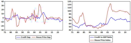
Figure 1. Growth of credit and house prices in South Africa.

South Africa’s real GDP growth statistics reflect this stagnation. After contracting by 7.0% in 2020 due to the pandemic, the economy rebounded with a growth of 4.9% in 2021, largely driven by a low base effect. However, growth slowed significantly in 2022, with real GDP expanding by only 2.0%, and projections for 2023 showed a meagre 1.1% growth. This post-pandemic recovery has been frail, hindered by persistent structural challenges in key sectors, such as power supply issues, weak private-sector investment, and, importantly, stagnation in credit and asset prices.

There is mounting evidence suggesting that financial variables such as credit growth and house prices are leading indicators of business cycles in South Africa. Boshoff and Fourie (2020) provide compelling evidence that credit and housing markets are important early signals of economic activity. Therefore, the sluggish recovery in these markets can be a key reason behind the prolonged stagnation of South Africa’s broader economic recovery. However, such observations based on visual inspection alone are not sufficient to draw firm conclusions. Formal testing, which is conducted in this study, is required to substantiate the relationship between financial variables and the overall economic recovery.

The study also contributes by employing a dynamic factor model to construct the real-financial activity gap, offering a more comprehensive measure of economic fluctuations that account for financial market conditions. This approach complements existing studies that have relied on the HP filter within the state-space framework, providing an alternative methodology that incorporates financial variables and real GDP in the estimation. Moreover, the study utilises the recursive augmented Dickey–Fuller (RADF) model to systematically identify statistically significant economic recoveries, distinguishing between genuine recoveries and those that lack statistical robustness. This method enhances the accuracy of detecting turning points in economic cycles, improving upon traditional unit root tests. Lastly, the study employs the Markov-switching dynamic regression model to formally date economic recoveries, capturing regime shifts and providing a more nuanced understanding of transitions between recessions and recoveries. Covering the period from 1970 to 2024, it offers a long-term perspective on financial and economic dynamics, enabling robust analysis of structural changes and policy implications over time.

The remainder of the study is structured as follows: Section 1 introduces the study. Section 2 reviews the relevant literature. Section 3 describes the data and methodology. Section 4 presents the results and discussion. Finally, Section 5 concludes the study.

2. Literature Review

The importance of financial variables in business cycle estimation has long been recognised in economic theory, with scholars emphasising the interaction between financial and real variables in measuring economic activity (Yan & Huang, 2020; Adarov, 2021; Jawadi et al., 2022). Historically, the role of financial factors in economic fluctuations was highlighted by early theorists such as Fisher (1933) and Keynes (1937), who argued that financial market conditions significantly influence the broader economy. Their insights were later supported by empirical evidence, which demonstrated that financial imbalances contribute to macroeconomic volatility (Afanasyeva et al., 2024; O’Brien & Velasco, 2025).

Fisher’s (1933) debt-deflation theory provided a compelling explanation for the Great Depression. It posits that, during economic booms, financial markets are flooded with liquidity, leading to excessive borrowing and speculative investments in risky assets (Parusel & Viegi, 2009; Hryhoriev, 2024). When asset prices begin to decline, firms and households struggle to service their debts, leading to widespread defaults and a contraction in credit availability. This process further depresses aggregate demand, exacerbating economic downturns. Empirical studies have confirmed the relevance of Fisher’s theory in explaining recent crises, including the 1990s’ Japanese asset price bubble and the 2008 global financial crisis (Bernanke & Gertler, 1999; Reinhart & Rogoff, 2014; Quiviger, 2020; Hryhoriev, 2023).

Similarly, Keynes’ (1937) general theory emphasised the role of credit availability and lender confidence in shaping economic activity. Keynes argued that fluctuations in financial markets impact aggregate demand through changes in investment spending (Mariati et al., 2022; Blackford, 2024). When confidence in the financial system deteriorates, credit tightens, leading to a decline in business investment and economic output (Gatti & Love, 2008; Krugman, 2001; Begg, 2023). This mechanism also proved invaluable for understanding the Great Depression, where a loss of confidence led to a dramatic contraction in credit and spending (Crockett, 1996; Calomiris et al., 2022). Empirical research supports Keynes’ insights, demonstrating that variations in credit conditions strongly influence economic growth patterns (Kim & Mehrotra, 2018; Pelsa & Balina, 2022; Patinkin, 2024).

On the other hand, the credit cycle theory developed by Kiyotaki and Moore (1997) highlights the interaction between asset prices and credit constraints in driving business cycle fluctuations (Mills, 2024). According to this theory, rising asset prices increase the net worth of firms, enabling them to borrow more and invest in further expansion. Conversely, declining asset values tighten credit constraints, leading to economic contraction. Empirical studies support this theory, showing that financial shocks often precede recessions (Z. Liu & Wang, 2014; Drehmann, 2013; Gulen et al., 2024). The credit cycle theory finds application in South Africa’s banking sector, as the 2015–2016 credit contraction, caused by rising interest rates and regulatory tightening, led to reduced investment and slower GDP growth (Mandipa & Sibindi, 2022; Tinbergen, 2024). This aligns with the notion that asset price fluctuations and credit constraints amplify business cycles (Z. Liu & Wang, 2014; Winkler, 2020). Additionally, empirical study by Azolibe et al. (2025) demonstrates that South African bank lending conditions influence private sector investment, further validating the role of financial variables in business cycle dynamics.

Another influential approach is the financial-economic cycle theory proposed by Bernanke et al. (1999) and Gertler and Karadi (2011). It suggests that credit conditions, including bank lending standards and risk perceptions, play a central role in economic fluctuations. When financial institutions tighten lending standards in response to perceived risks, investment and consumption decline, leading to slower economic growth. Studies (see Hubrich et al., 2013; C. Borio et al., 2014; Yang, 2023; Magubane, 2025) confirm this relationship, demonstrating that financial constraints can amplify business cycle fluctuations. For instance, during the 2008 crisis, South Africa witnessed a sharp decline in credit extension, increased loan defaults, and reduced aggregate demand, consistent with the debt-deflation theory (Aron & Muellbauer, 2013). Similarly, the SARB argued that financial imbalances, such as rising household debt and declining business confidence, have been significant predictors of economic slowdowns in South Africa (Magubane, 2024b).

The 1980s witnessed a shift away from financial considerations in macroeconomic modelling. The Modigliani-Miller theorem (1958) posits that a firm’s capital structure—whether financed by debt or equity—was irrelevant to its valuation, leading many economists to downplay the role of financial variables in business cycles (Gersbach & Papageorgiou, 2024; Brusov et al., 2021; Bossone, 2024). This perspective contributed to the failure of mainstream economic models to predict the 2007/09 financial crisis. Standard macroeconomic models, which focused primarily on real variables such as output and employment, overlooked the growing financial imbalances that ultimately triggered the crisis (C. Borio & Zhu, 2012; Correa-Jimenez et al., 2024). Studies show that financial indicators, such as rising private-sector leverage and credit booms, provided early warning signs of the crisis that conventional models failed to capture (Drehmann et al., 2012; C. E. Borio & Lowe, 2002; Kolte et al., 2021; Khan et al., 2022). This underscores a broader limitation in pre-crisis macroeconomic thinking, where financial markets were assumed to be largely self-correcting and of secondary importance to real economic dynamics.

Mainstream macroeconomic models have historically underappreciated the role of financial cycles in economic stability (Coban & Apaydin, 2025). C. Borio et al. (2017) and Yang (2023) argue that traditional models treated financial disturbances as temporary shocks rather than as fundamental drivers of business cycles. However, research increasingly suggests that financial cycles are longer and more pronounced than traditional business cycles, making them essential for understanding macroeconomic dynamics (Drehmann et al., 2012; Alessi & Detken, 2018; Cerra et al., 2023; Coimbra & Rey, 2024). The failure of pre-2007 macroeconomic models to predict the global financial crisis underscores the need to integrate financial and real variables in economic analysis. Empirical evidence from South Africa reinforces these theoretical insights. The economy has experienced financial-driven business cycles, particularly during the 1998 emerging market crisis, the 2008 global financial crisis, and the COVID-19 pandemic in 2020 (Magubane & Mncayi-Makhanya, 2025). These experiences align with international findings, demonstrating that periods of financial instability often precede economic downturns.

Empirically, the link between financial variables such as financial cycles and business cycles has been explored in various ways. Schularick and Taylor (2012), Rünstler and Vlekke (2018), Oman (2019), and Boehm and Kroner (2023) studied the attributes of business and financial cycles. These studies show that despite the financial cycle being longer in amplitude and less frequent, it still shares similar attributes with the business cycle, such as periods of expansions and downturns. However, these studies mostly focus on advanced economies. For example, Drehmann et al. (2012) analysed the characteristics of real GDP (business cycles) and financial cycles in the private credit market, asset market, and equity market in the seven largest advanced economies (Australia, Germany, the United Kingdom, Japan, Norway, Sweden, and the United States). Employing the Harding and Pagan concordance index and frequency-based filters, the study found evidence of longer financial cycles in contrast to shorter business cycles. According to Drehmann et al. (2012), the average business cycle lasts about ten years, while the average financial cycle takes about 30 years. A similar finding was also made by Claessens et al. (2011). Therefore, it can be rationally expected that financial events do not always coincide with business cycle events (Adarov, 2021).

Similar to Drehmann et al. (2012), Schüler et al. (2020) argue that financial cycles are distinct from business cycles. The latter authors found that financial cycles last 15 years on average, in contrast to an average of 9 years for business cycles in G-7 countries, excluding Japan. Rünstler and Vlekke (2018) analysed the attributes of business and financial cycles for the five largest European economies and found that the length of business and financial cycles differed by 7 years, with business cycles lasting up to 8 years, while financial cycles last up to 15 years. A similar finding was reached by Scharnagl and Mandler (2019). Stremmel (2015) found that financial cycles are four times larger than business cycles in the European Union (EU) member countries. These findings highlight that financial cycles are a distinct phenomenon from business cycles, especially in AEs (Agrippino & Rey, 2021). While the central bank primarily anchors its inflation-targeting framework to the business cycle, this focus may inadvertently overlook the slower-moving nature of financial cycles. Since monetary policy decisions such as adjustments to the repo rate are often made in response to short- to medium-term fluctuations in the business cycle, the economy experiences more frequent and rapid cyclical adjustments. In contrast, financial cycles evolve over a much longer horizon, as they are largely driven by factors such as financial innovation and technological developments that take time to diffuse through the economy. This temporal mismatch implies that policy decisions reacting to short-term business fluctuations may overlook emerging financial imbalances that build up over longer horizons. This disconnect underscores the importance of recognising that policy responses aligned solely with business cycles may fail to capture the broader, long-term dynamics of financial cycles (C. Borio, 2014).

Findings from South Africa largely align with those of advanced economies but also reveal unique attributes. Farrell and Kemp (2020) confirm the presence of a financial cycle in South Africa that is longer and has a larger amplitude than the business cycle, consistent with findings from international studies. Their study finds that credit and house prices are key indicators of the South African financial cycle, while the role of equity prices remains uncertain. The 2008 financial crisis illustrated this dynamic, as the collapse of housing prices led to a contraction in credit and a severe economic downturn (Bernanke et al., 1999; Miranda-Agrippino & Rey, 2022; Cerra et al., 2023).

Additionally, periods of financial stress coincide with financial cycle peaks, reinforcing international evidence that financial conditions serve as leading indicators of economic downturns. Similarly, Bosch and Koch (2020) established that the average South African financial cycle lasts approximately 17.3 years, which is significantly longer than the business cycle’s 5.8-year duration, echoing global trends. However, the observation that South Africa has not yet reached a deleveraging trough raises concerns when compared to international cases where financial cycles have typically completed full deleveraging after downturns.

Further research highlights the synchronisation of financial cycles in South Africa. Using the dynamic conditional correlation model and the vector error correction mechanism, Magubane (2024b) found strong correlations among financial cycles in South Africa, with intensification during financial crises. This suggests contagion effects similar to those observed in advanced economies. However, the financial and business cycles in South Africa exhibit a higher degree of synchronisation than those in advanced economies, resembling findings from Latin America and Southeast Asia. As a result, it remains debatable whether South Africa’s monetary and macroprudential frameworks can effectively operate as substitutes, given the country’s financial and policy stance (see Agénor & da Silva, 2019).

The synchronisation of business and financial cycles has rarely been explored in detail, yet it holds significant implications for the coordination of monetary and macroprudential policies (Rünstler & Vlekke, 2018; Nyati et al., 2023). When business and financial cycles are strongly synchronised, monetary and macroprudential policies can be used as substitutes. However, if the two cycles are not in sync, these policies should be employed as complementary tools (Oman, 2019; Mattera & Franses, 2023). The idea behind this distinction is that synchronised cycles suggest a unified path, meaning either monetary or macroprudential policy can ensure both price and financial stability. In contrast, a lack of synchronisation indicates diverging paths, necessitating a coordinated, simultaneous application of both policy tools to achieve stability (Agénor & da Silva, 2019; Chen & Phelan, 2024).

In a comparative analysis, Boshoff (2005) examined the leading indicator properties of multiple financial variables from 1986 to 2004, noting that while some financial variables synchronise well with business cycle phases, no single variable consistently serves as a reliable leading indicator for the South African business cycle. Interestingly, real M3 proved to be a superior leading indicator compared to M1, the measure currently employed by the South African Reserve Bank (SARB). However, local stock market indices were found to have a weakened correlation with economic activity, limiting their usefulness as composite leading indicators (Venter, 2020).

Pahla (2019) further examined South Africa’s financial cycle in relation to global factors, finding that domestic financial cycles are influenced by global financial conditions, particularly low global interest rates post-2007/09. The study reveals that the South African credit cycle is weakly countercyclical, indicating that business cycles may lead credit growth rather than the reverse, a distinction from some international findings where credit cycles often precede business cycles. Additionally, the South African financial cycle exhibits moderate co-movement with the global financial cycle and a stronger negative co-movement with the VIX, suggesting that while it is affected by global trends, it retains some idiosyncratic characteristics.

While these theoretical insights are well established, empirical studies addressing cycle synchronisation often neglect the temporal aspects, focusing instead on static models. A few notable studies, such as those by Claessens et al. (2011), Drehmann et al. (2012), Gomez-Gonzalez et al. (2015), and Clark (2024), have made efforts to examine the relationship between business and financial cycles, but they rely on methods like the Harding and Pagan (2006) concordance index and frequency domain analysis. These models, while helpful in identifying co-movement between cycles, often fail to capture the dynamic nature of their interactions, especially during periods of instability (Coimbra & Rey, 2024). Billio et al. (2017) introduced the dynamic influence Markov-switching dynamic factor model, which quantitatively captures interaction patterns and causal relationships between economic cycles. Building on this, Oman (2019) showed that financial cycles are generally less synchronised than business cycles, with notable differences across economies. More recently, Juhro et al. (2024) found that capital flow cycles often precede both financial and business cycles, emphasising the complexity of these interconnections. Nonetheless, the literature consistently underscores the difficulty of accurately modelling dynamic interactions, particularly during periods of financial instability.

Claessens et al. (2011) examined 700 business cycles and 400 financial cycles across OECD advanced economies from 1960 to 2017, and they found strong synchronisation between business and financial cycles in credit and housing markets, with deep recessions often coinciding with financial disruptions. Similarly, Gomez-Gonzalez et al. (2015) observed bidirectional Granger causality between credit and output cycles at medium frequencies, suggesting that these cycles are interconnected across both developed and emerging markets. Yet, the finding that business cycles are shorter than financial cycles complicates the idea that they always move together (Crispín et al., 2024). Moreover, some research aims to use financial cycle fluctuations to forecast business cycle events. For instance, C. Borio et al. (2017) and Mitchell (2024) studied the predictive power of financial cycles for recessions, finding that, during periods of financial expansion, the probability of a business cycle recession increases in the following three years. This aligns with the view that financial cycles often precede business cycles, particularly at turning points. Furthermore, studies suggest that as economies approach crises, business and financial cycles become more aligned (Oman, 2019; Stremmel & Zsámboki, 2015; Dafermos et al., 2023).

Further exploration of the interactions between business and financial cycles highlights that these cycles, despite their differences in length and amplitude, tend to influence each other positively. Lang and Welz (2018) and Tsiakas and Zhang (2023), for example, investigated the impact of economic factors on housing market financial gaps and found that potential GDP influences financial gaps in the housing market, leading to cycles lasting up to 15 years. Grintzalis et al. (2017) and Banerjee and Goyal (2024) also found that credit inflows from advanced economies (AEs) to emerging market economies (EMEs) cause fluctuations in output. These studies suggest a mutual influence between business and financial cycles, leading them to co-move over time.

Despite these efforts, static models such as the Harding and Pagan concordance index and frequency domain analysis fail to capture the complexities of cycle synchronisation, especially in unstable periods. While Claessens et al. (2011), Drehmann et al. (2012), Gomez-Gonzalez et al. (2015), Celov and Comunale (2022), and Chudziak (2025) highlight the co-movement of business and financial cycles; they do not sufficiently address how the timing of cycle phases affects synchronisation patterns. The persistence of differences in cycle durations and amplitudes further complicates the issue, calling for more dynamic approaches.

There are additional factors behind the distinction of the attributes exhibited by business and financial cycles, including the existence of financial frictions (Bernanke & Gertler, 1999; Bernanke et al., 1999; Kiyotaki & Moore, 1997; Miranda-Agrippino & Rey, 2022) and policy regimes (C. Borio, 2014; C. Borio et al., 2017; Cagliarini & Price, 2017). For instance, the shift towards more financially liberal economies since the 1980s has amplified the length and amplitude of financial cycles (C. E. Borio & Lowe, 2002). This is because, with more financial liberalisation, financial constraints are relaxed, thereby supporting full interplay between financial markets (C. Borio, 2014). This is why strong capital flows are also associated with strong financial booms. This further supports the idea that monetary policy alone cannot achieve both price and financial stability since financial cycles are strongly influenced by the financial regulatory regime in place (Miranda-Agrippino & Rey, 2022).

In this study, we combine both financial and real variables to construct a real-financial activity for South Africa. By integrating financial variables such as credit and house prices with real economic indicators, we aim to provide a more comprehensive measure of economic activity. This approach leverages the complementarity between business and financial cycles to capture a fuller picture of the economy’s performance, particularly in the aftermath of the COVID-19 pandemic and the global financial crisis. The real-financial activity gap allows us to better assess economic recoveries and downturns, distinguishing between those that are sustainable and those driven by financial imbalances. It also provides a more nuanced tool for policymakers to respond to emerging economic risks. The contributions of this study are threefold. Firstly, it extends the methodology of constructing business cycles by applying it to a South African context, an area that has received limited attention in the existing literature. Secondly, it offers a new approach to assessing economic recoveries by incorporating financial variables, enhancing our understanding of how these factors influence overall economic stability. Lastly, the study introduces formal testing to evaluate the role of finance-adjusted gaps in distinguishing between sustainable and unsustainable recoveries, addressing a critical gap in current research.

To test the robustness and relevance of the real-financial activity gap, the following null hypotheses are developed for this study:

• There is a real-financial activity gap for South Africa, implying that the inclusion of financial variables does not improve the measurement of the output gap.
• The real-financial activity gap does not distinguish between economic downturns and recoveries, suggesting that incorporating financial variables does not add predictive value for recovery dynamics.
• The real-financial activity gap is the same in duration, amplitude, volatility, and length as the traditional output gap, indicating that the finance-adjusted gap does not provide a more accurate or differentiated view of economic cycles compared to the traditional output gap.

These hypotheses will be tested using formal statistical methods to assess the validity and utility of incorporating financial variables into the construction of output gaps, ultimately contributing to the broader literature on business cycle analysis and policymaking in South Africa.

3. Methodology

3.1. Data and Definitions

The main aim of the study is to construct an economic measure that accounts for financial developments in South Africa. Thereafter, this cycle will be contrasted with the traditional business cycle in assessing its usefulness in predicting economic recoveries. In this study, we follow the growth deviation cycle definition of business cycles rather than the classical view. The traditional definition of business cycles describes fluctuations in a nation’s aggregate economic activity, marked by expansions, recessions, and contractions, which recur in a general pattern but are not strictly periodic (Burns & Mitchell, 1946; I. Mintz, 1972). These classical recessions, characterised by actual declines in output, have become rare, leading some scholars in the 1960s to question whether business cycles were a thing of the past (Mathews, 1968; N. N. Mintz, 1970).

However, the growth deviation cycle, as proposed by Lucas (1976), offers a more relevant framework for modern economies. This approach focuses on fluctuations around potential growth rather than outright declines. In this view, periods of below-potential growth are considered recessions, while periods of above-potential growth represent expansions. This model better reflects the experience of advanced economies, where output tends to grow over time, rendering classical recessions less frequent. In the literature, there is no agreed-upon definition for the real-financial activity gap. This study follows a definition that considers the finance-adjusted business cycle, which integrates financial market fluctuations with traditional economic activity cycles. This view recognises that financial instability can amplify or dampen the effects of business cycles, with financial booms and busts directly influencing expansions and contractions (C. Borio et al., 2017; Grintzalis et al., 2017).

In order to construct the traditional business cycle, the study utilises real gross domestic product (GDP) collected from the South African Reserve Bank. To construct the real-financial activity gap, real GDP will be combined with the ratio of credit to GDP (CR), house price index (HPI), and the all-share price index (SP). The ratios of credit to GDP and the house price index were both sourced from the Bank of International Settlements, whereas the all-share price index was sourced from the Organisation for Economic Cooperation and Development. Table 1 below provides a summary of variables. These financial variables were chosen for the purpose of this study because several studies have shown that their co-movement strongly correlates with the booms and busts of the financial system. As a result, credit and asset prices are widely regarded as the best representation of the financial developments (Drehmann et al., 2012; Claessens et al., 2012; Oman, 2019; Stremmel, 2015; Gorton & Ordoñez, 2016; Stremmel & Zsámboki, 2015). For instance, Oman (2019) highlights that leverage is strongly associated with credit and asset price movements. Additionally, Adarov (2021) shows that share prices and long-term interest rates are linked to credit and asset prices, reinforcing their role in capturing financial cycles, a view also supported by C. Borio et al. (2017). Therefore, financial cycles can be understood as the co-movement of various financial indicators that may culminate in system-wide booms and busts. Besides this, these variables represent the largest financial markets in South Africa, which are the credit and insurance market as well as the stock market (Magubane, 2024b). All variables were standardised using z-scores to ensure comparability.

Table 1. Summary of variables.

Variable	Definition	Source	Transformation
GPD	Real gross domestic product at market prices	South African Reserve Bank	z-score standardisation
CR	The ratio of total domestic credit to real gross domestic product	Bank of International Settlements	z-score standardisation
HPI	Real house price index	Bank of International Settlements	z-score standardisation
SP	All share price index	Organisation for Economic Cooperation and Development	z-score standardisation

3.2. Methods

The dynamic factor model (DFM) is employed to extract a common factor between real GDP and the financial variables. The dynamic factor model is a dimension-reduction technique summarising the sources of variation among variables (Doz & Fuleky, 2020). The model, although originally developed by Geweke (1978), over time, has been developed in various forms by various scholars (e.g., Sargent & Sims, 1977; Stock & Watson, 1989; Chamberlain, 1983; Koop & Korobilis, 2014; Del Negro & Otrok, 2008). Several good economic analyses have been done using the DFM; for instance, see Bai and Ng (2008), Bai and Wang (2016), Barigozzi (2022), Eickmeier and Breitung (2006), and Stock and Watson (2016). In the area of financial cycle analysis, it has been employed by D. Liu et al. (2020), Pahla (2019), and De Wet and Botha (2022). In this study, we use the DFM to achieve two things. Firstly, the DFM is used to extract a common factor describing joint variation between credit, house, and equity prices for each country. Secondly, the DFM is used to assess the importance of common factors vis-a-vis idiosyncratic factors in explaining variations in financial cycles to analyse how synchronised they are.

The DFM employed in this study is similar to Adarov (2023). Assume that the $n$-dimensional ($n=x$) stationary process $Y_{it},i=1,2\dots ,n$ (variables) can be decomposed into orthogonal unobservable components (Monfort et al., 2003; Moneta & Rüffer, 2009; Nieuwenhuyze, 2006). The unobserved components are factors that capture the common variation in variables and idiosyncratic factors, ${\epsilon }_{it }F$ actors that capture variations specific to each variable but propagate to other variables. It is important to note that although the latent factor affects all indicators simultaneously, its impact is heterogeneous across variables and, therefore, is captured by variable-specific factor loading. The DFM is specified as follows:

$$Y_t={\phi }_{it}{F}_t+{\epsilon }_{it}$$

(1)

Following the language of the Kalman filter, Equations (1) and (2) are referred to as a system of ($n\times 1$) measurement equations (Adarov, 2023), and Equation (4) below is a transition equation.

$$F_t={\chi }_t{F}_{t-1}+\cdots {\chi }_p{F}_{t-p}+{\eta }_t$$

(2)

where $F_t$ is ($k\times 1$) vector of factors, ${\phi }_t$ is a vector of factor loadings or coefficients measuring indicators’ sensitivity to common factors. ${\chi }_t$ is a ($k\times k)$ matrix of (P) coefficients, and ${\epsilon }_t$ and ${\eta }_t$ are error terms that carry the idiosyncratic influence (Stock & Watson, 2010). Furthermore, the study assumes that the error terms are independent, normally distributed, and orthogonal with the covariance matrices $cov\left({\epsilon }_t\right)=Q; cov\left({\eta }_t\right)=R; cov\left({\epsilon }_t,{\eta }_t\right)=0$. Q is the identity matrix, and $R$ is a diagonal matrix with equal variances along the main diagonal. In classic factor models, specific components are assumed to be uncorrelated, limiting their usefulness (Nzimande & Ngalawa, 2019). Forni and Lippi (2001) argue that while the orthogonality assumption of idiosyncratic factors is essential for identification purposes, it is a restrictive assumption. Indeed, within the context of this study, the assumption is not appropriate since financial cycles are interlinked. As such, changes in the financial cycle $x$ can induce changes in the financial indicator $y$ in a way that is closely ‘cross-regressive’, so that a cycle-specific shock originating in the indicator $x$ transmits, with a lag, to the indicator $y$ (Adarov, 2023; Forni & Lippi, 2001). Therefore, this study allows the specific components to be weakly and cross-sectionally correlated to some degree, as in Forni et al. (2004).

To estimate the model, the study follows De Jong (1991) and Hamilton et al. (2016); it uses the Kalman filtering technique to estimate the Gaussian likelihood and the parameters, yielding efficient estimates of the factors. The first step in implementing this approach is to cast the dynamic factor model into a linear space model (Stock & Watson, 2010). Let $F_t={(f}_t^{\prime },f_{t-1}^{\prime },\dots ,f_{t-p}^{\prime })$ represent $(r\times 1)$ vector, let $p$ be the extent of lag polynomials matrix $\Phi \left(L\right),$ and let $\Omega =({\Phi }_0{\Phi }_1,\dots ,{\Phi }_p$ where $\Phi$ is the $(N\times q)$ matrix of coefficients on the $i_{t}h$ lag in $\Phi \left(L\right).$ Also, let $\Psi \left(L\right)$ be the matrix of 1’s and 0’s, and the components of $\chi \left(L\right)$ such that the VAR in equations three and four can be written as follows:

$$Y_{it}=\Omega F_t+{ϵ}_t$$

(3)

$$\Psi \left(L\right)F_t=G{v}_t$$

(4)

where $G$ is a matrix of 1’s and 0’s selected to ensure that Equations (1) and (4) are common. We complete this new representation by specifying the law of motion for ${ϵ}_t$. Thus, ${ϵ}_t$ is assumed to follow a univariate autoregressive process:

$$d_i\left(L\right){ϵ}_t={\eta }_{i}t,i=1,\dots , N$$

(5)

Therefore, Equations (5)–(7) constitute a comprehensive linear state space model. Given the parameters, we exploit the Kalman filter to generate the likelihood and estimate the filtered values of $F_t$ and therefore of $f_t$.

To determine the optimal number of factors (k) and lag length (p) in the dynamic factor model (DFM), we followed the approach proposed by Bai and Ng (2008). The number of factors was selected using their information criteria (IC₁, IC₂, and IC₃), which balance model fit and parsimony. The results consistently indicated that a single common factor (k = 1) sufficiently captures the co-movement between the real and financial variables in the dataset. This finding aligns with previous studies (e.g., Stock & Watson, 2016; Forni et al., 2004), which also find that one dominant factor explains most of the variation in macro-financial aggregates. The lag length (p) in the transition equation was determined using the Akaike (AIC) and Bayesian (BIC) information criteria, both of which favoured a first-order specification (p = 1). These choices ensure a parsimonious yet robust model specification suited for medium-sized quarterly datasets.

As pointed out earlier, this study uses the deviation cycles of Lucas (1976). Therefore, GDP is decomposed into two components: the cyclical and the secular. There exist voluminous filtering techniques in the literature, each with its own attributes. Hence, the discussion of their performance is ignored. The study employs, for comparability purposes, the Hodrick–Prescott filter, which is widely used in the business cycles literature (Lestano & Kuper, 2016; Nzimande & Ngalawa, 2019; Adarov, 2021; Drehmann & Yetman, 2018, among others).

For the purposes of the study, assume that the real-financial activity gap and real GDP are as follows:

$$y_t={\epsilon }_t+{\alpha }_{t}t=1,2\dots ,T$$

(6)

where $y_t$ is the observed series, GDP or the common factor from the DFM, ${\epsilon }_t$ and ${\alpha }_t$ are the trend component and cyclical component of the observed series, respectively. It is, moreover, assumed that the secular component is difference stationary, whereas the cyclical component is stationary at levels.

An estimate of the trend is obtained by minimising Equation (4):

$$\underset{{\left[g_t\right]}_{t=1}^T}{\min }{\sum }_{t=1}^T[{\left(y_t-{\epsilon }_t\right)}^2+\mathsf{\lambda }\left({\epsilon }_{t+1}-{\epsilon }_t\right)-{\left({\epsilon }_{t-1}-{\epsilon }_t\right)}^2]$$

(7)

where $\mathsf{\lambda }$ is the penalty parameter, which is closely related to the smoothness of the estimated trend. The penalty parameter is set to $\mathsf{\lambda }=1600$ for quarterly data, as suggested by Hodrick and Prescott (Lestano & Kuper, 2016). The HP-filtered log of real GDP represents the business cycle (BC). In addition to real GDP, the H-P filter is also applied to the common factor obtained in the DFM to produce the real-financial activity gap.

The Hodrick–Prescott (HP) filter (Hodrick & Prescott, 1997) is renowned for its ability to extract a smooth trend component from a time series, thereby isolating the cyclical component that represents fluctuations around the underlying trend. Since the trend and cyclical components are typically latent, the HP filter serves to approximate them through a minimisation process that balances the series’ deviation from its trend with the smoothness of that trend. A pivotal feature of this methodology is the smoothing parameter λ, which penalises excessive variations in the trend component. For quarterly data, a λ value of 1600 is recommended by Hodrick and Prescott (1997), a position later supported by Marcet and Ravn (2004). To capture the longer duration of financial cycles, the Basel Committee on Banking Supervision, following the approach of Drehmann et al. (2012), recommends using a higher smoothing parameter of λ = 400,000 for quarterly data. For monthly data, Zarnowitz and Ozyildirim (2006) propose a baseline λ of 108,000, and when adjusted using the conversion factor suggested by Drehmann et al. (2012) to reflect the extended financial cycle length, a suitable smoothing parameter becomes λ = 27,648,000.

While the HP filter is widely used and offers clear practical advantages, it is not without limitations. Chief among these are the end-point bias—where the trend is less reliable at the sample’s beginning and end—and the sensitivity of the extracted cycle to the chosen λ value. These limitations mean that care must be taken when interpreting the results, as minor changes in the smoothing parameter or sample period can affect the precise timing of peaks and troughs. Nonetheless, the HP filter remains the most practical and empirically validated detrending method available, particularly for studies seeking comparability with international work on financial and business cycles. Its use is further justified by policy relevance: institutions such as the Bank for International Settlements (BIS) continue to recommend the HP filter for the analysis of cyclical behaviour in financial and macroeconomic variables.

Empirical studies also support its application. Drehmann and Yetman (2018), Dritsaki and Dritsaki (2022), Siemers (2024), and Alfaro and Drehmann (2023) have all found that the HP filter outperforms alternative detrending methods in approximating economic and financial cycles. Furthermore, within the South African context, previous research shows that the choice of detrending method does not significantly alter the qualitative features of financial cycles: Nyati et al. (2021) demonstrate that cycles derived using the Baxter-King (BK) filter are virtually identical to those obtained using the HP filter, a finding corroborated by Bosch and Koch (2020). These results affirm both the robustness and practical suitability of the HP filter for this study, while also underscoring the importance of cautious interpretation in light of its known sensitivities.

The RADF is used to date economic events predicted by the RFAG and the output gap. The RADF has been developed over time in studies such as Dickey and Fuller (1979), Phillips et al. (2011) and Phillips et al. (2015). The RADF calculates three tests that are based on the ADF regression with a constant:

$$∆y_t={\alpha }_{r_1,r_2}+{\beta }_{r_1,r_2}{y}_{t-1}+{\sum }_{i=1}^k{\delta }_{r_1,r_2}^i∆y_{-y_{t-i}}+{\epsilon }_t$$

(8)

where $∆$ is the first difference operator, $y_t$ is the realisation of the time series that is the traditional business cycle and the finance-adjusted output gap at time $t$, $k$ is a scalar that denotes the number of lags of the dependent variable that are included to account for residual serial correlation, and $r_1$ and $r_2$ denote the start and the end of the estimations, respectively. $r_1$ and $r_2$ are expressed as a fraction of the total number of periods $T$ in the entire sample such that $r_2=r_1=r_w$ where $r_w$ is the window size of the regression also expressed as a fraction of $T$. The number of observations used to estimate 8 is denoted as $T_w=\left[T_{r_w}\right]$ where $\left[T\right]$ is the floor function, which gives the integer part of its argument. The error term is ${\epsilon }_t$.

The unit root null hypothesis is given by $H_0:{\beta }_{r1,r_2}=0$ while the alternative hypothesis is that the series of interest exhibits explosive behaviour, i.e., $H_1:{\beta }_{r_1,r_2}>0$. While the augmented Dickey–Fuller (ADF) test is useful for detecting non-stationary processes, its power to detect explosive behaviour is limited, particularly in the presence of collapsing bubbles or short-lived episodes of exuberance. To address this limitation, the methodology introduces recursive variations of the ADF test that are better suited to identify episodes of explosive growth. The supremum ADF (SADF) test, as developed by Phillips et al. (2011), extends the ADF test by recursively estimating the test statistic over expanding subsamples of the data. The SADF statistic is calculated as the supremum of the ADF t-statistics computed over a range of recursive windows. In practice, the SADF test begins by estimating the ADF regression on a small initial sample, then progressively increases the size of the sample window while recalculating the ADF statistic. The supremum ADF statistic is then used to test for explosive behaviour across the entire sample period. This approach allows the SADF test to detect periods of exuberance that may not persist for the entire duration of the sample.

However, the SADF test has a limitation in that it is designed to detect only the first instance of explosive behaviour, potentially missing subsequent bubbles that may occur within the sample. To overcome this, the methodology incorporates the general supremum ADF (GSADF) test, as proposed by Phillips et al. (2015). The GSADF test generalises the SADF procedure by allowing both the starting and ending points of the recursive sample window to vary. This flexibility enables the GSADF test to detect multiple episodes of explosive behaviour within the same series. Specifically, the GSADF statistic is calculated by running a series of ADF regressions over all possible subsample windows and taking the supremum of the resulting ADF t-statistics. This approach significantly enhances the ability of the test to capture multiple explosive episodes, making it particularly useful in analysing time series with complex dynamics, such as asset price bubbles that collapse and re-emerge.

The inference for both the SADF and GSADF tests relies on the comparison of the calculated test statistics against critical values derived from the distribution of the test under the null hypothesis of no explosive behaviour. These critical values are typically obtained through Monte Carlo simulations, where a large number of random walks are generated under the assumption of a unit root. The simulated distributions provide the basis for determining the critical values at different significance levels (e.g., 90%, 95%, 99%) for the SADF and GSADF statistics.

An important aspect of the methodology is the treatment of heteroskedasticity, which can distort the size and power of the tests. To address this issue, the methodology incorporates a wild bootstrap procedure, as recommended by Phillips and Shi (2020). The wild bootstrap is a resampling technique that generates bootstrap replications of the time series by perturbing the residuals in the ADF regression using random draws from a predefined distribution. This approach helps to mitigate the effects of unconditional heteroskedasticity, which can otherwise lead to size distortions in the test. Additionally, the bootstrap provides a means of accounting for the multiplicity of tests conducted in the recursive framework, ensuring that the critical values used in the SADF and GSADF tests are robust to these factors.

In practical terms, the methodology is implemented using the radf command in STATA, which allows users to compute the ADF, SADF, and GSADF statistics for a given time series. The command supports various options for determining the lag length in the ADF regression, either through user specification or via data-dependent criteria such as the Akaike information criterion (AIC) or Schwarz information criterion (SIC). Users can also specify the window width for the recursive estimations, although the default settings follow the recommendations of Phillips et al. (2015). The radf command further provides functionality for generating and graphing sequences of t-statistics, along with the corresponding critical values, enabling a visual representation of episodes of explosive behaviour.

Output gaps have two phases, i.e., expansions and contractions. They transition between these two phases. Accordingly, the MSDR is used in this study to corroborate the findings of the RADF. The model is adopted here because it provides attractive transition features over a set of finite states (Buthelezi, 2023). It allows the transition process to evolve differently in each state. The transition occurs according to a Markov process. The time of transition from one state to another and the duration between changes in the state are random (Hansen, 2000). The MSDR has been applied by Nyati et al. (2021) and De Wet and Botha (2022) to study the features of financial cycles in South Africa. Assume a financial cycle can be denoted by $y_t$ where $t=1,2\dots ,T$ is characterised by two states, then a financial cycle can be presented in Equations (9) and (10) as follows:

$$State1:y_t={\mu }_1+{ϵ}_t$$

(9)

$$State2:y_t={\mu }_2+{ϵ}_t$$

(10)

where ${\mu }_1$ and ${\mu }_2$ are state-dependent means in $State1$ and $State2$ respectively, and ${ϵ}_t$ is a white noise error with variance ${\sigma }^2$. The two-state model shifts in the mean term. If the timing of switches is known, the above model can be expressed as follows:

$$y_t=s_t{\mu }_1+\left(1-s_t\right){\mu }_2+{ϵ}_t$$

(11)

The subscript $s_t$ is the transition process in state 1 and 0 otherwise. The Markov switching regression model allows the parameters to vary over the unobserved states. The MSDR model with state-dependent mean is reflected in Equation (12):

$$y_t={\mu }_{s_t}+{ϵ}_t$$

(12)

where ${\mu }_{s_t}$ is the parameter of interest; ${\mu }_{s_t}={\mu }_1$ when $s_t=1$ and ${\mu }_{s_t}={\mu }_2$ when $s_t=2.$ The probabilities of being in each state can be estimated with transition probabilities (Buthelezi, 2023). One-step transition probabilities are given by $P{s}_t, s_t+1$. For a two-state process, $p_{11}$ denotes the probability of staying in state 1 in the next period, given that the process is in state 1 in the current period. $p_{22}$ denotes the probability of staying in state 2 in the next period, given the process is in state 2 in the current period. The transition probabilities from one state to another can be presented in matrix form:

$$P=\left(\begin{array}{cc}{p}_{11}& p_{12}\\ p_{21}& p_{22}\end{array}\right)$$

(13)

4. Results

4.1. RADF Results

This section presents the results of the RADF test, which was used to examine the null hypothesis of unit roots against the alternative hypothesis of explosive behaviour across the entire sample. The results are displayed in Table 2. In the table, a rejection of the null hypothesis in favour of the alternative is indicated when the $t$-statistic exceeds both the Monte Carlo critical values (RTMC) and the right-tail tabulated critical values (Tab). RFAG refers to the real-financial activity gap, while BC refers to the business cycle or the output gap.

Table 2. RADF main results.

		t-Statistic	RTMC90	RTMC95	RTMC99	Tab90	Tab95	Tab99
RFAG	ADF0	3.1506	−0.3670	0.0012	0.6427	−0.3754	−0.0150	0.6270
	SADF	4.0293	1.3764	1.7905	3.1702	1.0994	1.3915	1.9502
	GSADF	4.0293	2.8607	3.5494	4.6613	1.8590	2.1135	2.5811
BC	ADF0	−5.0464	−0.5505	−0.1431	0.4520	−0.3754	−0.0150	0.6270
	SADF	0.7870	2.2726	2.5625	3.3300	1.0994	1.3915	1.9502
	GSADF	3.4571	3.7118	3.9772	4.9566	1.8590	2.1135	2.5811

Notes: RFAG refers to the real-financial activity gap, while BC refers to the business cycle. RTMC refers to Monte Carlo critical values, while Tab refers to right-tailed tabulated critical values. 90, 95, and 99 refer to the 10%, 5%, and 1% levels of significance, respectively. ADF refers to the augmented Dickey–Fuller, SADF refers to the supremum augmented Dickey–Fuller, and general supremum augmented Dickey–Fuller.

A close inspection of Table 2 reveals that the $t$-statistics for the ADF, SADF, and GSADF tests consistently exceed their corresponding RTMC and tab critical values. This indicates a rejection of the null hypothesis, confirming the presence of explosive behaviour in the series. These findings underscore the predictive value of the real-financial activity gap in identifying periods of economic recovery in South Africa. This result is consistent with previous research that demonstrated how financial variables provide valuable information for forecasting economic activity in South Africa (Venter, 2020; Aye et al., 2019; Brogaard & Detzel, 2015; Boshoff & Fourie, 2020). These financial variables include variables such as interest rates, credit spreads, stock prices, and bank lending data that capture forward-looking dynamics that are not always reflected in traditional economic indicators such as GDP or unemployment. These variables react more swiftly to changes in market sentiment, liquidity conditions, and risk perceptions (Stock & Watson, 2003). For example, widening credit spreads or declining stock prices can signal tightening financial conditions or rising uncertainty, both of which tend to precede economic slowdowns (Adrian et al., 2010). Furthermore, financial variables are closely tied to the availability of credit, which plays a central role in investment and consumption decisions. When financial markets face stress, borrowing costs rise for businesses and consumers, leading to reduced spending and investment, ultimately slowing economic growth (Bernanke & Gertler, 1999).

Incorporating financial variables into forecasting models allows researchers to detect these shifts earlier, improving the accuracy of predictions of economic turning points, particularly during periods of uncertainty or crisis. Empirical studies consistently find that including financial market data enhances forecast precision (Reinhart & Rogoff, 2011; Aye et al., 2019). By integrating financial variables into the output gap measure for South Africa, this study ensures that crucial financial information is incorporated, thereby reducing the likelihood of false signals often associated with traditional business cycle indicators.

Next, the RADF test was conducted to examine the unit root null hypothesis against the alternative of explosive behaviour across the entire sample period. The results are presented in Figure 2 and Table 3. In Figure 2, the red lines represent the RTMC 95% critical value, while the blue lines depict the GSADF $t$-statistic. The figure reveals that both the real-financial activity gap and the traditional business cycle exhibit episodes of explosive behaviour, with the former displaying five such instances and the latter showing four. These episodes correspond to periods of economic recovery in South Africa, and they are clearly identifiable when the $t$-statistic exceeds the critical value.

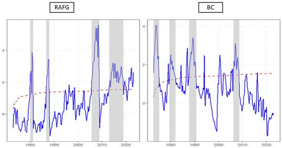
Figure 2. RADF economic recoveries. Notes: red dotted lines represent the RTMC 95% critical value, while the blue lines depict the GSADF t-statistic. RAFG refers to the real-financial activity gap, and BC refers to the business cycle. The grey shaded lines refers to the duration of boom phases of RFAG and the business cycle.

Table 3. RADF economic recoveries.

RAFG:
	Start	End	Duration
1	1 January 1980	1 April 1981	5
2	1 October 1986	1 January 1988	5
3	1 October 2005	1 January 2009	13
4	1 January 2013	1 January 2019	24
5	1 April 2021		9
BC:
	Start	End	Duration
1	1 October 1972	1 April 1975	10
2	1 July 1979	1 January 1982	10
3	1 October 1987	1 October 1990	12
4	1 April 2006	1 October 2008	10

Notes: RAFG refers to the real-financial activity gap, and BC refers to the business cycle.

When examining the shaded areas in Figure 2 and the details in Table 3, the dates of these recoveries are as follows: For the real-financial activity gap, the first episode of explosive behaviour occurred between 1 January 1980 and 1 April 1981. The second took place from 1 October 1986 to 1 January 1988. The third recovery began on 1 October 2005 and lasted until 1 January 2009. The fourth episode started on 1 January 2013 and ended shortly before the onset of the COVID-19 pandemic on 1 January 2019. Interestingly, both the figure and table suggest that the real-financial activity gap signals the beginning of a new economic recovery in the aftermath of the COVID-19 pandemic, a trend not observed in the traditional output gap.

In contrast, the traditional business cycle displays recoveries at different intervals. The first recovery occurred between 1 October 1972 and 1 April 1975. The second occurred from 1 July 1979 to 1 January 1982. The third recovery spanned 1 October 1987 to 1 October 1990, and the fourth took place between 1 April 2006 and 1 October 2008. Notably, the traditional business cycle does not indicate any recovery following the global financial crisis in 2007/2009. Figure 2 and Table 3 also highlight that, in recent years, the recoveries shown by the real-financial activity gap tend to last longer than those depicted by the traditional business cycle. Economic recoveries portrayed by the traditional business cycle typically last up to 10 quarters (approximately 2.5 years). In contrast, the recovery associated with the real-financial activity gap, beginning in 2005, lasted for 13 quarters (roughly three years). The recovery that started in 2013 was even longer, lasting 24 quarters (approximately five years). This suggests that the real-financial activity gap provides more extended recoveries, particularly in the aftermath of financial disruptions such as the global financial crisis and the COVID-19 pandemic.

The results that show longer economic recoveries for the real-financial activity gap compared to the traditional business cycle in South Africa can be justified using both economic theory and empirical evidence. The real-financial activity gap, which integrates financial market indicators with real economic variables, captures broader and slower-moving dynamics that extend the duration of recovery phases. According to the financial accelerator theory (Bernanke et al., 1999), financial conditions magnify and propagate economic shocks through credit and asset-price channels. When financial markets begin to recover after a downturn, improving balance sheets and easier access to credit stimulate investment and consumption, thereby sustaining expansion for longer periods than what is reflected by real output alone.

Empirical data from South Africa strongly supports this interpretation. For example, during the 2002/2008 expansion, private sector credit grew at an average annual rate of 14%, driven by rapid increases in household mortgage lending and corporate borrowing. Over this same period, domestic credit to the private sector rose from 71% of GDP in 2001 to approximately 142% of GDP by 2007—one of the highest ratios in South Africa’s post-apartheid history. This financial boom persisted for nearly six consecutive years, supported by rising asset prices on the Johannesburg Stock Exchange (the JSE All Share Index increased by over 230% between 2003 and 2007) and by a surge in household consumption financed by credit. Real GDP, by contrast, expanded at a more moderate average annual rate of 4.8% and began to decelerate sharply by late 2008 as global conditions deteriorated. Hence, while the real economy’s upswing lasted about 24 quarters, the financial boom and its recovery effects stretched closer to 30–32 quarters, continuing to support aggregate demand even as output growth slowed.

A similar divergence appeared in the post-2009 recovery. After the global financial crisis, South Africa’s real GDP rebounded quickly—rising by 4.9% in 2011—but the momentum faded by 2013 as investment and consumption weakened. Credit growth, however, followed a more prolonged and uneven path. Household debt-to-income ratios remained high (around 61%–63% between 2010 and 2014), and corporate credit continued expanding at about 8 to 10% annually well into 2015, long after real output growth had slowed to below 2%. This indicates that the financial recovery extended almost five to six years, while the real recovery was effectively exhausted after three years. More recently, following the COVID-19 recession of 2020, output rebounded by 4.9% in 2021 but then slowed to 1.9% in 2023. Financial conditions, however, improved more gradually: private sector credit, which contracted in 2020, began rising steadily by 4 to 6% per year between 2022 and 2025, with total credit reaching R5.1 trillion by September 2025 (a 6% year-on-year increase, driven mainly by corporate lending). This recovery in financial variables continues even as GDP growth remains subdued, again showing that the financial cycle—and therefore the real-financial activity gap—has a longer recovery trajectory than the traditional business cycle.

According to C. Borio (2014), the financial regime—defined by the degree of financial liberalisation, monetary policy stance, and institutional depth—plays a crucial role in determining the duration and amplitude of financial conditions. In the South African case, the post-apartheid liberalisation of capital markets, deepening of domestic credit markets, and flexible inflation-targeting regime established since 2000 have all contributed to lengthening the financial cycle. As financial integration increased, recoveries became more dependent on the restoration of credit and asset market conditions. This structural evolution means that South Africa’s economic expansions are now increasingly shaped by the financial regime itself—where monetary easing, credit expansion, and asset revaluation collectively prolong the recovery phase relative to the traditional, output-based business cycle.

Taken together, these episodes illustrate that financial recoveries in South Africa often outlast and out-amplify real ones. While output typically regains its pre-crisis level within two to three years, financial conditions—credit, asset prices, and balance sheet repair—take 5–8 years to normalise. The real-financial activity gap, therefore, provides a more realistic measure of the economy’s underlying recovery momentum, capturing the extended influence of financial sector dynamics that sustain growth long after the conventional business cycle has peaked.

The real-financial activity gap’s ability to indicate that South Africa entered an economic recovery following the COVID-19 pandemic, while the traditional business cycle shows no recovery from the global financial crisis of 2007/09, can also be explained by the role of financial markets in modern economies. The COVID-19 pandemic led to unprecedented global monetary and fiscal responses, including interest rate cuts and quantitative easing, which helped stabilise financial markets and foster recovery. South Africa, like many emerging economies, implemented accommodative monetary policies that supported financial markets, even amid the real sector’s downturn. These measures may not have been fully captured by the traditional business cycle approach, which focuses on real economy indicators, but were reflected in the real-financial activity gap.

In contrast, during the 2007/09 global financial crisis, South Africa experienced a more muted recovery in financial markets, with less accommodative monetary policy, higher interest rates, and more constrained credit markets (Aron & Muellbauer, 2013). As a result, the traditional business cycle does not show a strong recovery after this period, which aligns with the slow pace of economic recovery globally. The real-financial activity gap, by capturing both real and financial dynamics, is more sensitive to these shifts in monetary policy and financial market conditions, thereby better reflecting the post-COVID-19 recovery, while the absence of financial market stabilisation in 2007/09 leads to no recovery being detected.

Moreover, the data on South Africa’s economic performance supports these conclusions. South Africa’s GDP growth averaged 2.6% from 2005 to 2008 before contracting sharply during the financial crisis, whereas the post-COVID recovery saw growth bounce back from a 7% contraction in 2020 to a 4.9% rebound in 2021. This faster rebound post-pandemic, spurred by aggressive financial policies, explains why the real-financial activity gap detects a recovery following COVID-19, while the global financial crisis period lacked such momentum.

4.2. MSDR Main Results

The MSDR was employed to corroborate the findings of the RADF. We now turn to the results of the MSDR, which are presented in Table 4. In this table, subscript 1 refers to state 1, while subscript 2 refers to state 2. An evaluation of the state-dependent mean, μ, indicates that state 1 corresponds to economic downturns, whereas state 2 corresponds to recovery. This is reflected in the relationship that μ_2 > μ_1. The duration parameter, φ, shows that economic events characterised by the real-financial activity gap have a longer duration compared to those indicated by the traditional business cycle, reinforcing the findings of the RADF. Specifically, economic recoveries represented by the real-financial activity gap last up to 31 quarters, which is approximately six years. In contrast, recoveries depicted by the traditional business cycle last up to 19 quarters, roughly four years. The transition probabilities of remaining in economic recovery, represented as ρ_22 = 0.954 and ρ_21 = 0.949, are both close to 1, indicating that economic recoveries are persistent. This suggests a high likelihood of remaining in the recovery state once it is reached. Additionally, the variances, σ_2 = 0.558 and σ_1 = 0.011, suggest that the real-financial activity gap is associated with more volatile economic recoveries compared to the traditional business cycle. This perennial finding implies that the real-financial activity gap is able to capture and even forecast economic recoveries characterised by high volatility, which the traditional business cycle may fail to detect. This capability is particularly important because periods of over-indebtedness, excessive borrowing, and an accommodative policy stance during an economic boom can sow the seeds of the subsequent crisis.

Table 4. MSDR main results.

	RFAG	BC
${\mu }_1$	−0.742 ***	−0.001 *
${\mu }_2$	0.501 ***	0.001
${\sigma }_1$	0.361 **	0.003 *
${\sigma }_2$	0.558 **	0.011 ***
${\rho }_{11}$	0.935	0.929
${\rho }_{12}$	0.065	0.071
${\rho }_{21}$	0.046	0.051
${\rho }_{22}$	0.954	0.949
${\phi }_1$	15.317	9.082
${\phi }_2$	31.676	19.397

Notes: RAFG refers to the real-financial activity gap, and BC refers to the business cycle. $\mu , \sigma , \rho , \phi$ refer to state mean, state variance, transition probabilities, and state duration, respectively. The subscripts 1 and 2 denote downturns and recovery states, respectively. ***, **, and * refer to the p-values at the 1%, 5% and 10% level of significance, respectively.

To justify this finding, take the following examples. Prior to the 2008/2009 financial crisis in South Africa, the traditional business cycle suggested a stable economy. Real GDP was growing at robust rates of around 4.6% in 2004 and 5.4% in 2007, and conventional indicators such as employment and capacity utilisation showed no imminent risk. In contrast, financial conditions were signalling increasing volatility and systemic fragility. Private sector credit was expanding rapidly at roughly 25.1% year-on-year by April 2007 while the ratio of domestic credit to the private sector as a share of GDP reached approximately 142%. Household debt-to-income ratios climbed from around 69.4% in 2006 to 76% in early 2007 and peaked at 82% in the first quarter of 2008. reflecting rising leverage and growing financial vulnerability. Asset markets, including property and equity prices, were also highly volatile, exhibiting large swings in valuations. A similar pattern occurred earlier during the 2002 small banks crisis, when several smaller commercial banks experienced liquidity stress due to overexposure to risky loans, even though GDP growth at the time remained moderate and the broader business cycle did not indicate systemic weakness. These episodes indicate that the financial sector can accumulate risk and exhibit volatility well before downturns become visible in the real economy. This divergence demonstrates that the real-financial activity gap captures recoveries characterised by heightened volatility—periods of expansion that are inherently fragile and prone to reversal—whereas traditional output-based business cycle measures fail to detect these latent vulnerabilities.

Besides the above, empirical studies on South Africa have shown that the business cycle often behaves as a lagging indicator, responding to shocks only after they have affected output and employment, whereas financial variables—such as credit growth, asset prices, and leverage—tend to act as leading indicators (Aron & Muellbauer, 2013). Consequently, the RFAG, by incorporating these financial variables alongside real activity, is better positioned to detect building volatility in the economy and to provide early warning signals of potential crises, while traditional output-based measures typically register these vulnerabilities only after they have materialised.

In addition to increased volatility, the real-financial activity gap demonstrates greater persistence in economic recoveries. Research by Jordà et al. (2013) highlights that post-crisis recoveries often unfold slowly, particularly when initial downturns are linked to financial disturbances. High levels of household and corporate debt create an environment where consumers and businesses are hesitant to spend, leading to subdued demand and prolonged recovery periods. This persistent economic weakness is not adequately captured by traditional output gap calculations, which typically assume a more rapid return to potential output. The real-financial activity gap, therefore, serves as a more realistic measure of recovery, accounting for the time required to stabilise financial conditions and restore confidence in the economy.

Ultimately, these findings emphasise the importance of integrating financial analysis into economic assessments to formulate effective policy responses. Policymakers need to recognise that economic recovery is not solely dependent on traditional supply and demand factors; it is significantly influenced by the underlying health of financial systems. By adopting a real-financial activity gap framework, policymakers can better understand the volatility and persistence of recoveries, allowing for more targeted interventions. This holistic approach to economic analysis not only enhances our comprehension of output gaps but also facilitates the development of strategies aimed at achieving sustainable economic growth and stability in the face of financial uncertainty.

Next, we turn to the dating of economic recoveries using the MSDR. Figure 3 and Table 5 present the dates. MSDR indicates that RAFG experienced recoveries during 1981Q1–1986Q2, 1989Q1–1992Q2, 1996Q3–2000Q1, 2005Q1–2009Q3, 2010Q4–2016Q1, 2017Q4–2020Q3, and 2021Q1–2023Q2. In comparison, BC recoveries occurred in 1970Q1–1973Q3, 1974Q4–1977Q3, 1980Q1–1983Q2, 1994Q3–1997Q1, 2000Q1–2003Q1, 2005Q1–2009Q3, 2010Q4–2016Q1, 2017Q4–2020Q3, and 2021Q1–2023Q2. RADF results roughly correspond to these periods but show notable differences. In comparison, for RAFG, RADF recoveries include periods such as 1980/01–1981/04 (5 quarters), 1986/10–1988/01 (5 quarters), 2005/10–2009/01 (13 quarters), 2013/01–2019/01 (24 quarters), and 2021/04–2021/12 (9 quarters), while BC recoveries occur in 1972/10–1975/04, 1979/07–1982/01, 1987/10–1990/10, and 2006/04–2008/10. This indicates that RADF tends to detect shorter, more punctuated recovery periods, often starting earlier or ending sooner than those captured by MSDR, whereas MSDR captures longer, regime-confirmed expansions that reflect sustained recoveries.

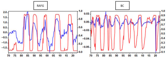
Figure 3. MSDR state probabilities. Notes: The blue lines represent RAFG and BC. The red lines represent the probabilities of entering a recovery phase.

Table 5. MSDR economic recoveries.

RAFG		BC
Date	Duration	Date	Duration
1981Q1–1986Q2	28	1970Q1–1973Q3	15
1989Q1–1992Q2	20	1974Q1–1977Q3	15
1996Q3–2000Q1	20	1980Q1–1983Q2	14
2004Q4–2012Q2	36	1984Q1–1986Q4	12
2016Q2–2020Q1	24	1988Q4–1992Q3	16
		1994Q3–1999Q1	19
		2000Q1–2003Q1	13
		2005Q1–2009Q3	19
		2010Q4–2016Q1	22
		2017Q4–2020Q3	12
		2021Q1–2023Q2	10

Notes: RAFG refers to the real-financial activity gap, and BC refers to the business cycle.

The differences between the two models can be explained by their underlying properties. RADF is designed to identify periods of explosive behaviour in time series, making it highly sensitive to early signals of recovery or temporary surges, even if they are not fully persistent. In contrast, MSDR identifies structural regime shifts, capturing persistent changes in the underlying economic process and effectively filtering out short-term fluctuations. This property explains why RADF sometimes signals recoveries earlier or for shorter durations, while MSDR produces longer, smoother recovery periods that reflect confirmed regime changes. Both models are therefore reliable within their respective frameworks: RADF excels at providing early warnings, while MSDR delivers robust confirmation of sustained economic shifts.

Specific examples illustrate these differences. For RAFG, MSDR indicates a recovery beginning in 1981Q1, while RADF shows an earlier start in 1980/01 (≈1980Q1), likely reflecting early signs of recovery in real-financial activity. MSDR, in contrast, identifies recovery only once the regime has entered a sustained expansion. For BC, MSDR shows recovery in 2005Q1–2009Q3, whereas RADF reports 2005/10–2009/01, capturing short-term fluctuations before the economy stabilises fully. Importantly, RAFG often signals recoveries earlier than BC, highlighting the predictive advantage of combining financial and real variables. This observation aligns with studies indicating that financial factors frequently lead the real economy (e.g., Drehmann et al., 2012; Schularick & Taylor, 2012). Moreover, RADF recoveries tend to be shorter in duration, emphasising temporary surges that may not persist, whereas MSDR recoveries are longer, reflecting regimes with inertia and persistence.

For policymakers, these mixed signals should be treated as complementary rather than conflicting. RADF provides timely, high-frequency indications that may signal early intervention points, while MSDR offers confirmation of sustained economic recoveries. By considering both models together, policymakers can respond proactively to emerging trends without overreacting to transient fluctuations, ensuring that interventions are both timely and grounded in structural evidence. Overall, the combination of RADF and MSDR enhances the reliability of recovery assessments and strengthens the policy toolkit for managing complex dynamics in both financial and real sectors.

5. Conclusions

This study aimed to construct a finance-output-adjusted gap for South Africa and utilise it to predict the occurrence of economic recoveries. Given that recoveries precede downturns, understanding their timing and frequency is essential for policymakers to anticipate and mitigate subsequent downturns. To achieve this, the study examined the period from 1970Q1 to 2023Q4, incorporating real GDP, domestic credit, house prices, and share prices. A dynamic factor model and the Hodrick–Prescott filter were used to construct the finance-adjusted gap, while the recursive ADF unit root test assessed the frequency and duration of economic recoveries. To validate the findings, a Markov switching dynamic regression model was employed to analyse the volatility of economic recoveries, transition probabilities from downturns to recoveries, and recovery durations in South Africa.

The findings of this study reinforce the growing body of literature that emphasises the significance of integrating financial variables into traditional business cycle analysis to enhance predictive accuracy. Prior studies have shown that financial developments influence economic fluctuations and that neglecting these factors can lead to underestimations of recovery dynamics (C. Borio, 2014; Drehmann et al., 2012). The results of this research align with these insights, demonstrating that the real-financial activity gap provides a more stable and extended view of economic recoveries compared to real GDP-based predictions, which tend to suggest shorter but more frequent recoveries. This underscores the need to refine economic forecasting models by incorporating financial cycle dynamics.

For practitioners and policymakers, these findings have several critical implications. Firstly, understanding that financial variables contribute to prolonged but less frequent recoveries suggests that stabilising credit and asset price growth can help smooth economic cycles and reduce abrupt downturns. Policymakers, particularly central banks and financial regulators, should closely monitor financial indicators alongside traditional macroeconomic measures to better anticipate economic recoveries and mitigate future recessions. Additionally, financial stability measures—such as macroprudential policies—can be designed to manage excessive credit growth and asset price inflation, fostering more resilient economic recoveries.

Despite its contributions, this study has certain limitations. The real-financial activity gap, while incorporating key financial indicators, may still omit other critical factors such as global financial spillovers, geopolitical risks, and behavioural finance aspects, which could further refine recovery predictions. Additionally, the reliance on the Hodrick–Prescott filter and dynamic factor model assumes a relatively stable relationship between financial and real economic variables, which may not fully capture structural changes over time.

Future research should explore more granular financial indicators, such as sector-specific credit conditions or household and corporate leverage dynamics, to improve the accuracy of recovery predictions. Additionally, expanding the analysis to other emerging markets and systemic advanced economies could provide a comparative perspective on how financial conditions shape recoveries within different economic contexts. Further work could also integrate machine learning techniques to enhance forecasting models and test their robustness under varying macroeconomic conditions.

Overall, this study contributes to the evolving discourse on financial cycle dynamics by highlighting the predictive power of real-financial activity gaps. By incorporating financial variables into economic recovery analysis, this research provides a valuable tool for policymakers seeking to design more effective stabilisation policies and navigate the complexities of modern economic cycles.

References

- Adarov, A. (2021). Dynamic interactions between financial cycles, business cycles and macroeconomic imbalances: A panel VAR analysis. International Review of Economics & Finance, 74, 434–451. [Google Scholar] [CrossRef]
- Adarov, A. (2023). Financial cycles in Europe: Dynamics, synchronicity and implications for business cycles and macroeconomic imbalances. Empirica, 50, 551–583. [Google Scholar] [CrossRef]
- Adrian, T., Estrella, A., & Shin, H. S. (2010). Monetary cycles, financial cycles, and the business cycle. Technical Report, Staff Report. Federal Reserve Bank of New York. [Google Scholar]
- Afanasyeva, E., Jerow, S., Lee, S. J., & Modugno, M. (2024). Sowing the seeds of financial imbalances: The role of macroeconomic performance. Journal of Financial Stability, 74, 100839. [Google Scholar] [CrossRef]
- Agénor, P. R., & da Silva, L. A. P. (2019). Integrated inflation targeting—Another perspective from the developing world. Available online: https://www.bis.org/publ/othp30.pdf (accessed on 16 November 2025).
- Agrippino, S. M., & Rey, H. (2021). The global financial cycle. NBER Working Paper, (w29327). Available online: https://www.nber.org/papers/w29327 (accessed on 16 November 2025).
- Aikman, D., Giese, J., Kapadia, S., & McLeay, M. (2019). Targeting financial stability: Macroprudential or monetary policy? (ECB Working Paper). Bank of England. [Google Scholar]
- Akar, C. (2016). Analyzing the synchronization between the financial and business cycles in Turkey. Journal of Review on Global Economics, 5, 25–35. [Google Scholar] [CrossRef]
- Albarrán Macías, D., Mejía Reyes, P., & López Herrera, F. (2022). Synchronization of the business cycles of Mexico and the United States: A dynamic correlation approach. Investigación Económica, 81(319), 37–62. [Google Scholar] [CrossRef]
- Aldasoro, I., Avdjiev, S., Borio, C. E., & Disyatat, P. (2020). Global and domestic financial cycles: Variations on a theme. BIS. [Google Scholar]
- Alessi, L., & Detken, C. (2018). Identifying excessive credit growth and leverage. Journal of Financial Stability, 35, 215–225. [Google Scholar] [CrossRef]
- Alfaro, R., & Drehmann, M. (2023). The Holt–Winters filter and the one-sided HP filter: A close correspondence. Economics Letters, 222, 110925. [Google Scholar] [CrossRef]
- Aron, J., & Muellbauer, J. (2013). Wealth, credit conditions, and consumption: Evidence from South Africa. Review of Income and Wealth, 59, S161–S196. [Google Scholar] [CrossRef]
- Aye, G. C., Christou, C., Gil-Alana, L. A., & Gupta, R. (2019). Forecasting the probability of recessions in South Africa: The role of decomposed term spread and economic policy uncertainty. Journal of International Development, 31, 101–116. [Google Scholar] [CrossRef]
- Azolibe, C. B., Dimnwobi, S. K., & Uzochukwu-Obi, C. P. (2025). The determinants of unemployment rate in developing economies: Does banking system credit matter? Journal of Economic and Administrative Sciences, 41(1), 300–319. [Google Scholar] [CrossRef]
- Bai, J., & Ng, S. (2008). Large dimensional factor analysis. Foundations and Trends® in Econometrics, 3, 89–163. [Google Scholar] [CrossRef]
- Bai, J., & Wang, P. (2016). Econometric analysis of large factor models. Annual Review of Economics, 8, 53–80. [Google Scholar] [CrossRef]
- Banerjee, K., & Goyal, A. (2024). New perspectives on the rise and fall of global imbalances: Evidence from large emerging market economies. Review of World Economics, 160(2), 541–583. [Google Scholar] [CrossRef]
- Barigozzi, M. (2022). On estimation and inference of large approximate dynamic factor models via the principal component analysis. arXiv, arXiv:2211.01921. [Google Scholar]
- Batóg, J. A., & Batóg, B. (2019). Synchronization of business cycles in the EU: Time series clustering. WSEAS Transactions on Business and Economics, 16, 298–305. [Google Scholar]
- Bauer, G., Pasricha, G., Sekkel, R., & Terajima, Y. (2018). The global financial cycle, monetary policies, and macroprudential regulations in small, open economies. Canadian Public Policy, 44, 81–99. [Google Scholar] [CrossRef]
- Begg, H. M. (2023). Global banks in national markets: A theory of post-crisis reform as democracies under constraint [Doctoral dissertation, University of Oxford]. [Google Scholar]
- Berger, M. H., Dowling, M. T., Lanau, M. S., Mrkaic, M. M., Rabanal, M. P., & Sanjani, M. T. (2015). Steady as she goes—Estimating potential output during financial “booms and busts”. International Monetary Fund. [Google Scholar]
- Bernanke, B. S. (2018). The real effects of disrupted credit: Evidence from the global financial crisis. Brookings Papers on Economic Activity, 2018, 251–342. [Google Scholar] [CrossRef]
- Bernanke, B. S., & Gertler, M. (1999). Inside the black box: The credit channel of monetary policy transmission. Journal of Economic Perspectives, 9, 27–48. [Google Scholar] [CrossRef]
- Bernanke, B. S., Gertler, M., & Gilchrist, S. (1999). The financial accelerator in a quantitative business cycle framework. Handbook of Macroeconomics, 1, 1341–1393. [Google Scholar]
- Bernhofer, D., Fernández-Amador, O., Gächter, M., & Sindermann, F. (2014). Finance, potential output and the business cycle: Empirical evidence from selected advanced and CESEE economies. Focus on European Economic Integration, 2, 52–75. [Google Scholar]
- Bilan, Y., Brychko, M. M., Buriak, A. V., & Vasylieva, T. A. (2019). Financial, business and trust cycles: The issues of synchronization. Zbornik Radova Ekonomskog Fakulteta u Rijeci: Časopis za Ekonomsku teoriju i Praksu/Proceedings of Rijeka Faculty of Economics: Journal of Economics and Business, 37(1), 113–138. [Google Scholar] [CrossRef]
- Billio, M., Donadelli, M., Paradiso, A., & Riedel, M. (2017). Which market integration measure? Journal of Banking & Finance, 76, 150–174. [Google Scholar] [CrossRef]
- Blackford, G. H. (2024). Causality in economics and Keynes’ general theory. Real-World Economics Review, 1(109), 84–107. [Google Scholar]
- Boehm, C. E., & Kroner, T. N. (2023). The US, economic news, and the global financial cycle. Review of Economic Studies, 1, rdaf020. [Google Scholar]
- Borio, C. (2014). The financial cycle and macroeconomics: What have we learnt? Journal of Banking & Finance, 45, 182–198. [Google Scholar] [CrossRef]
- Borio, C., Disyatat, P., & Juselius, M. (2017). Rethinking potential output: Embedding information about the financial cycle. Oxford Economic Papers, 69, 655–677. [Google Scholar] [CrossRef]
- Borio, C., Drehmann, M., & Tsatsaronis, K. (2014). Stress-testing macro stress testing: Does it live up to expectations? Journal of Financial Stability, 12, 3–15. [Google Scholar] [CrossRef]
- Borio, C., & Zhu, H. (2012). Capital regulation, risk-taking and monetary policy: A missing link in the transmission mechanism? Journal of Financial Stability, 8(4), 236–251. [Google Scholar] [CrossRef]
- Borio, C. E., & Lowe, P. W. (2002). Asset prices, financial and monetary stability: Exploring the nexus. Available online: https://www.bis.org/publ/work114.htm (accessed on 16 November 2025).
- Bosch, A., & Koch, S. F. (2020). The South African financial cycle and its relation to household deleveraging. South African Journal of Economics, 88(2), 145–173. [Google Scholar] [CrossRef]
- Boshoff, W. H. (2005). The properties of cycles in South African financial variables and their relation to the business cycle. South African Journal of Economics, 73(4), 694–709. [Google Scholar] [CrossRef]
- Boshoff, W. H., & Fourie, J. (2020). Business cycles and structural change in South Africa. Springer. [Google Scholar]
- Bossone, B. (2024). A Modigliani-Miller theorem for the public finances of globalized economies. International Review of Financial Analysis, 94, 103257. [Google Scholar] [CrossRef]
- Brogaard, J., & Detzel, A. (2015). The asset-pricing implications of government economic policy uncertainty. Management Science, 61, 3–18. [Google Scholar] [CrossRef]
- Brusov, P., Filatova, T., Orekhova, N., Kulik, V., Chang, S. I., & Lin, G. (2021). Generalization of the Modigliani–Miller theory for the case of variable profit. Mathematics, 9(11), 1286. [Google Scholar] [CrossRef]
- Burns, A. F., & Mitchell, W. C. (1946). Measuring business cycles. National Bureau of Economic Research. [Google Scholar]
- Buthelezi, E. M. (2023). Impact of government expenditure on economic growth in different states in South Africa. Cogent Economics & Finance, 11, 2209959. [Google Scholar] [CrossRef]
- Cagliarini, A., & Price, F. (2017). Exploring the link between the macroeconomic and financial cycles|conference–2017. Available online: https://www.rba.gov.au/publications/confs/2017/pdf/rba-conference-volume-2017-cagliarini-price.pdf (accessed on 16 November 2025).
- Calomiris, C. W., Jaremski, M., & Wheelock, D. C. (2022). Interbank connections, contagion and bank distress in the Great Depression. Journal of Financial Intermediation, 51, 100899. [Google Scholar] [CrossRef]
- Celov, D., & Comunale, M. (2022). Business cycles in the EU: A comprehensive comparison across methods. In Essays in honour of Fabio Canova (Vol. 44, pp. 99–146). Emerald Publishing Limited. [Google Scholar]
- Cerra, V., Fatás, A., & Saxena, S. C. (2023). Hysteresis and business cycles. Journal of Economic Literature, 61(1), 181–225. [Google Scholar] [CrossRef]
- Chamberlain, G. (1983). Funds, factors, and diversification in arbitrage pricing models. Econometrica: Journal of the Econometric Society, 51(5), 1305–1323. [Google Scholar] [CrossRef]
- Chen, W., & Phelan, G. (2024). Liquidity provision and financial stability. Journal of Money, Credit and Banking, 56(2–3), 455–487. [Google Scholar] [CrossRef]
- Chiarini, B., Ferrara, M., & Marzano, E. (2022). Tax evasion and financial accelerator: A corporate sector analysis for the US business cycle. Economic Modelling, 108, 105780. [Google Scholar] [CrossRef]
- Chudziak, S. (2025). Economic dynamics may be different than it seems: Multiplicity of relevant economic cycles. SGH KAE. [Google Scholar]
- Claessens, S., Kose, M. A., & Terrones, M. E. (2011, May). Financial cycles: What? How? When? In NBER international seminar on macroeconomics. (Vol. 7, No. 1, pp. 303–344). University of Chicago Press. [Google Scholar]
- Claessens, S., Kose, M. A., & Terrones, M. E. (2012). How do business and financial cycles interact? Journal of International Economics, 87, 178–190. [Google Scholar] [CrossRef]
- Clark, J. M. (2024). Business acceleration and the law of demand: A technical factor in economic cycles. In Classics in institutional economics, part II (Vol. 6, pp. 24–43). Routledge. [Google Scholar]
- Coban, M. K., & Apaydin, F. (2025). Navigating financial cycles: Economic growth, bureaucratic autonomy, and regulatory governance in emerging markets. Regulation & Governance, 19(1), 126–145. [Google Scholar]
- Coimbra, N., & Rey, H. (2024). Financial cycles with heterogeneous intermediaries. Review of Economic Studies, 91(2), 817–857. [Google Scholar] [CrossRef]
- Correa-Jimenez, A., Davies, R., & Siddique, R. (2024). Macroeconomic modelling: A review. Available online: https://economicsobservatory.com/Macroeconomic_Modelling_Review.pdf (accessed on 16 November 2025).
- Crispín, Á. R. M., Silva, M. O. C., Villarrue, M. M. Á. L., & Pérez, M. W. M. C. (2024). The business cycle and the financial cycle: Granger causality for the Peruvian economy, 2000–2019. Journal of Ecohumanism, 3(4), 2582–2595. [Google Scholar] [CrossRef]
- Crockett, A. (1996). The theory and practice of financial stability. De Economist, 144(4), 531–568. [Google Scholar] [CrossRef]
- Dafermos, Y., Gabor, D., & Michell, J. (2023). Institutional supercycles: An evolutionary macro-finance approach. New Political Economy, 28(5), 693–712. [Google Scholar] [CrossRef]
- De Groot, O. (2021). A financial accelerator through coordination failure. The Economic Journal, 131, 1620–1642. [Google Scholar] [CrossRef]
- De Jong, P. (1991). The diffuse Kalman filter (pp. 1073–1083). The Annals of Statistics. [Google Scholar]
- Del Negro, M., & Otrok, C. (2008). Dynamic factor models with time-varying parameters: Measuring changes in international business cycles. FRB of New York Staff Report. Federal Reserve Bank of New York. [Google Scholar]
- De Wet, M. C., & Botha, I. (2022). Constructing and characterising the aggregate South African financial cycle: A Markov regime-switching approach. Journal of Business Cycle Research, 18, 37–67. [Google Scholar] [CrossRef]
- Dickey, D. A., & Fuller, W. A. (1979). Distribution of the estimators for autoregressive time series with a unit root. Journal of the American Statistical Association, 74, 427–431. [Google Scholar]
- Doz, C., & Fuleky, P. (2020). Dynamic factor models. In Macroeconomic forecasting in the era of big data: Theory and practice (pp. 27–64). Springer. [Google Scholar]
- Drehmann, M. (2013, June). Total credit as an early warning indicator for systemic banking crises. BIS Quarterly Review. Available online: https://www.bis.org/publ/qtrpdf/r_qt1306f.htm (accessed on 16 November 2025).
- Drehmann, M., Borio, C. E., & Tsatsaronis, K. (2012). Characterising the financial cycle: Don’t lose sight of the medium term! BIS. [Google Scholar]
- Drehmann, M., & Yetman, J. (2018). Why you should use the Hodrick–Prescott filter–at least to generate credit gaps. BIS. [Google Scholar]
- Dritsaki, M., & Dritsaki, C. (2022, July). Modelling and forecasting GDP of Greece with a modified exponential smoothing state space framework. In International conference on applied economics (pp. 89–110). Springer International Publishing. [Google Scholar]
- Eickmeier, S., & Breitung, J. (2006). How synchronized are new EU member states with the euro area? Evidence from a structural factor model. Journal of Comparative Economics, 34, 538–563. [Google Scholar] [CrossRef]
- El-Baz, O. (2018). The synchronization of financial and business cycles in Saudi Arabia. Scholedge International Journal of Management & Development, 5, 32–47. [Google Scholar] [CrossRef][Green Version]
- Epure, M., Mihai, I., Minoiu, C., & Peydró, J.-L. (2024). Global financial cycle, household credit, and macroprudential policies. Management Science, 70, 8096–8115. [Google Scholar] [CrossRef]
- Farrell, G., & Kemp, E. (2020). Measuring the financial cycle in South Africa. South African Journal of Economics, 88(2), 123–144. [Google Scholar] [CrossRef]
- Fisher, I. (1933). The debt-deflation theory of great depressions. Econometrica: Journal of the Econometric Society, 1, 337–357. [Google Scholar] [CrossRef]
- Forni, M., Hallin, M., Lippi, M., & Reichlin, L. (2004). The generalized dynamic factor model consistency and rates. Journal of Econometrics, 119, 231–255. [Google Scholar] [CrossRef]
- Forni, M., & Lippi, M. (2001). The generalized dynamic factor model: Representation theory. Econometric Theory, 17, 1113–1141. [Google Scholar] [CrossRef]
- Foroni, C., Marcellino, M., & Stevanovic, D. (2022). Forecasting the COVID-19 recession and recovery: Lessons from the financial crisis. International Journal of Forecasting, 38, 596–612. [Google Scholar] [CrossRef] [PubMed]
- Gatti, R., & Love, I. (2008). Does access to credit improve productivity? Evidence from Bulgaria 1. Economics of Transition, 16(3), 445–465. [Google Scholar] [CrossRef]
- Gersbach, H., & Papageorgiou, S. (2024). Bank influence at a discount. Journal of Financial and Quantitative Analysis, 59(6), 2970–3000. [Google Scholar] [CrossRef]
- Gertler, M., & Karadi, P. (2011). A model of unconventional monetary policy. Journal of monetary Economics, 58(1), 17–34. [Google Scholar] [CrossRef]
- Geweke, J. (1978). Temporal aggregation in the multiple regression model. Econometrica: Journal of the Econometric Society, 46, 643–661. [Google Scholar] [CrossRef]
- Giri, F., Riccetti, L., Russo, A., & Gallegati, M. (2019). Monetary policy and large crises in a financial accelerator agent-based model. Journal of Economic Behavior & Organization, 157, 42–58. [Google Scholar] [CrossRef]
- Gomez-Gonzalez, J. E., Villamizar-Villegas, M., Zarate, H. M., Amador, J. S., & Gaitan-Maldonado, C. (2015). Credit and business cycles: Causal effects in the frequency domain. Ensayos sobre Política Económica, 33(78), 176–189. [Google Scholar] [CrossRef]
- Gorton, G., & Ordoñez, G. (2016). Fighting crises. Technical Report. National Bureau of Economic Research. [Google Scholar]
- Grintzalis, I., Lodge, D., & Manu, A.-S. (2017). The implications of global and domestic credit cycles for emerging market economies: Measures of real-financial activity gaps. (ECB Working Paper). Bank of England. [Google Scholar]
- Gulen, H., Ion, M., Jens, C. E., & Rossi, S. (2024). Credit cycles, expectations, and corporate investment. The Review of Financial Studies, 37(11), 3335–3385. [Google Scholar] [CrossRef]
- Hamilton, F., Berry, T., & Sauer, T. (2016). Ensemble Kalman filtering without a model. Physical Review X, 6, 011021. [Google Scholar] [CrossRef]
- Hansen, B. E. (2000). Sample splitting and threshold estimation. Econometrica, 68, 575–603. [Google Scholar] [CrossRef]
- Harding, D., & Pagan, A. (2006). Synchronization of cycles. Journal of Econometrics, 132(1), 59–79. [Google Scholar] [CrossRef]
- Hodrick, R. J., & Prescott, E. C. (1997). Postwar US business cycles: An empirical investigation. Journal of Money, Credit, and Banking, 29, 1–16. [Google Scholar] [CrossRef]
- Hryhoriev, H. (2023, December 22). Debt deflation and world economic growth: System dynamics approach. 6th Annual International Research Conference (pp. 30–36), Kyiv, Ukraine. [Google Scholar]
- Hryhoriev, H. (2024). Debt deflation theory and middle-income trap: System dynamics approach. Scientific Papers NaUKMA Economics, 9(1), 24–31. [Google Scholar] [CrossRef]
- Hubrich, K., d’Agostino, A., Cervena, M., Ciccarelli, M., Guarda, P., Haavio, M., Jeanfils, P., Mendicino, C., Ortega, E., Valderrama, M. T., & Valentinyiné Endrész, M. (2013). Financial shocks and the macroeconomy: Heterogeneity and non-linearities. (No. 143. ECB Occasional Paper). European Central Bank. [Google Scholar]
- Iacoviello, M. (2015). Financial business cycles. Review of Economic Dynamics, 18, 140–163. [Google Scholar] [CrossRef]
- Jawadi, F., Ameur, H. B., Bigou, S., & Flageollet, A. (2022). Does the real business cycle help forecast the financial cycle? Computational Economics, 60(4), 1529–1546. [Google Scholar] [CrossRef]
- Jordà, Ò., Schularick, M., & Taylor, A. M. (2013). When credit bites back. Journal of Money, Credit and Banking, 45, 3–28. [Google Scholar] [CrossRef]
- Jordà, Ò., Schularick, M., Taylor, A. M., & Ward, F. (2018). Global financial cycles and risk premiums. Technical Report. National Bureau of Economic Research. [Google Scholar]
- Juhro, S. M., Iyke, B. N., & Narayan, P. K. (2024). Capital flow dynamics and the synchronization of financial cycles and business cycles in emerging market economies. Journal of International Financial Markets, Institutions and Money, 92, 101980. [Google Scholar] [CrossRef]
- Kalemli-Ozcan, S., Papaioannou, E., & Peydró, J.-L. (2009). Financial integration and business cycle synchronization. National Bureau of Economic Research. [Google Scholar]
- Keynes, J. M. (1937). The general theory of employment. The Quarterly Journal of Economics, 51(2), 209–223. [Google Scholar] [CrossRef]
- Khan, A. B., Zulfaqar, M., Iqbal, J., Hatim, M., & Faisal, M. A. (2022). Global financial crisis 2008–2009, macroeconomic variables and the performance of FTSE Bursa Malaysia Hijrah Shariah Index: A case of Malaysian stock market. Hamdard Islamicus, 43(1), 94–99. [Google Scholar]
- Kim, S., & Mehrotra, A. (2018). Effects of monetary and macroprudential policies—evidence from four inflation targeting economies. Journal of Money, Credit and Banking, 50(5), 967–992. [Google Scholar] [CrossRef]
- Kiyotaki, N., & Moore, J. (1997). Credit cycles. Journal of Political Economy, 105, 211–248. [Google Scholar] [CrossRef]
- Kolte, A., Roy, J. K., Patil, D. T., Pawar, A., & Sharma, P. (2021, March 17–18). Global financial crisis in 21st century: A brief analysis of stock exchanges. 2021 International Conference on Computational Intelligence and Knowledge Economy (ICCIKE) (pp. 290–295), Dubai, United Arab Emirates. [Google Scholar]
- Koop, G., & Korobilis, D. (2014). A new index of financial conditions. European Economic Review, 71, 101–116. [Google Scholar] [CrossRef]
- Kovačić, Z., & Vilotić, M. (2017). Assessing European business cycles synchronization. MPRA. [Google Scholar]
- Krugman, P. (2001, March 25–26). Crises: The next generation. Conference Honoring Assaf Razin, Tel Aviv, Israel. [Google Scholar]
- Lang, J. H., & Welz, P. (2018). Semi-structural credit gap estimation. (No. 2194. ECB Working Paper). Bank of England. [Google Scholar]
- Lestano, L., & Kuper, G. H. (2016). Correlation dynamics in East Asian financial markets. Emerging Markets Finance and Trade, 52, 382–399. [Google Scholar] [CrossRef]
- Liu, D., Sun, W., & Zhang, X. (2020). Is the Chinese economy well positioned to fight the COVID-19 pandemic? The financial cycle perspective. Emerging Markets Finance and Trade, 56, 2259–2276. [Google Scholar] [CrossRef]
- Liu, Z., & Wang, P. (2014). Credit constraints and self-fulfilling business cycles. American Economic Journal: Macroeconomics, 6(1), 32–69. [Google Scholar] [CrossRef]
- Lucas, R. E., Jr. (1976, January). Econometric policy evaluation: A critique. In Carnegie-Rochester conference series on public policy (Vol. 1, pp. 19–46). North-Holland. [Google Scholar]
- Magubane, K. (2024a). Exploring causal interactions between macroprudential policy and financial cycles in South Africa. International Journal of Research in Business & Social Science, 13(5), 513–531. [Google Scholar]
- Magubane, K. (2024b). Financial cycles synchronisation in South Africa. A dynamic conditional correlation (DCC) Approach. Cogent Economics & Finance, 12, 2321069. [Google Scholar]
- Magubane, K. (2025). The stability of the financial cycle: Insights from a Markov switching regression in South Africa. Journal of Risk and Financial Management, 18(2), 76. [Google Scholar] [CrossRef]
- Magubane, K., & Mncayi-Makhanya, P. (2025). The dynamic influence of the global financial cycle: Synchronization and impact on South Africa’s financial cycle. Cogent Economics & Finance, 13, 2451051. [Google Scholar] [CrossRef]
- Maliszewski, W., & Zhang, M. L. (2015). China’s growth: Can goldilocks outgrow bears? International Monetary Fund. [Google Scholar]
- Mandipa, G., & Sibindi, A. B. (2022). Financial performance and working capital management practices in the retail sector: Empirical evidence from South Africa. Risks, 10(3), 63. [Google Scholar] [CrossRef]
- Marcet, A., & Ravn, M. O. (2004). The HP-filter in cross-country comparisons. Available online: https://papers.ssrn.com/sol3/papers.cfm?abstract_id=511369 (accessed on 16 November 2025).
- Mariati, W., Yuesti, A., & Tahu, G. P. (2022). Economic growth based on the Keynes theory. International Journal of Sustainability, Education, and Global Creative Economic (IJSEGCE), 5(2), 61–72. [Google Scholar]
- Mathews, R. L. (1968). Finance for education. Economic Papers: A Journal of Applied Economics and Policy, 1(27), 1–30. [Google Scholar] [CrossRef]
- Mattera, R., & Franses, P. H. (2023). Are African business cycles synchronized? Evidence from spatio-temporal modeling. Economic Modelling, 128, 106485. [Google Scholar] [CrossRef]
- Mills, J. (2024). On credit cycles and the origin of commercial panics. In Business cycle theory, part I volume 1 (pp. 55–88). Routledge. [Google Scholar]
- Mintz, I. (1972). Dating American growth cycles. In Economic research: Retrospect and prospect, volume 1, the business cycle today (pp. 39–88). NBER. [Google Scholar]
- Mintz, N. N. (1970). Monetary union and economic integration. CJ Devine Institute of Finance, Graduate School of New York University. [Google Scholar]
- Miranda-Agrippino, S., & Rey, H. (2022). The global financial cycle. In Handbook of international economics (Vol. 6, pp. 1–43). Elsevier. [Google Scholar]
- Mitchell, W. C. (2024). Business cycles. In Business cycle theory, part II volume 8 (pp. 225–241). Routledge. [Google Scholar]
- Moneta, F., & Rüffer, R. (2009). Business cycle synchronisation in East Asia. Journal of Asian Economics, 20, 1–12. [Google Scholar] [CrossRef]
- Monfort, A., Renne, J.-P., Rüffer, R., & Vitale, G. (2003, November). Is economic activity in the G7 synchronized? Common shocks versus spillover effects. CEPR. [Google Scholar]
- Muthu, K., & Wesson, N. (2023). The impact of COVID-19 on company performance per industry sector: Evidence from South Africa. Journal of Economic and Financial Sciences, 16, 801. [Google Scholar] [CrossRef]
- Nieuwenhuyze, C. V. (2006). A generalised dynamic factor model for the Belgian economy-Useful business cycle indicators and GDP growth forecasts. (National Bank of Belgium Working Paper). National Bank of Belgium.
- Nyati, M. C., Muzindutsi, P. F., & Tipoy, C. K. (2023). Macroprudential and monetary policy interactions and coordination in South Africa: Evidence from business and financial cycle synchronization. Economies, 11(11), 272. [Google Scholar] [CrossRef]
- Nyati, M. C., Tipoy, C. K., & Muzindutsi, P.-F. (2021). Measuring and testing a modified version of the South African financial cycle. Economic Research Southern Africa Cape Town. [Google Scholar]
- Nzimande, N., & Ngalawa, H. (2019). Fiscal policy sustainability in SADC countries. African Finance Journal, 21, 86–97. [Google Scholar]
- O’Brien, M., & Velasco, S. (2025). Macro-financial imbalances and cyclical systemic risk dynamics: Understanding the factors driving the financial cycle in the presence of non-linearities. Macroeconomic Dynamics, 29, e13. [Google Scholar] [CrossRef]
- Oliviero, T., & Puopolo, G. W. (2021). Financial accelerator framework. In A modern guide to financial shocks and crises (pp. 45–64). Edward Elgar Publishing. [Google Scholar]
- Oman, W. (2019). The synchronization of business cycles and financial cycles in the euro area. International Journal of Central Banking, 15, 327–362. [Google Scholar]
- Pahla, Z. M. (2019). The determinants of the South African financial cycle. University of Johannesburg (South Africa). [Google Scholar]
- Parusel, M., & Viegi, N. (2009). Economic policy in turbulent times. Citeseer. [Google Scholar]
- Patinkin, D. (2024). ‘The Chicago Tradition, the Quantity Theory and Friedman’. In Keynes, Chicago and Friedman, volume 1 (pp. 85–120). Routledge. [Google Scholar]
- Pelsa, I., & Balina, S. (2022). Development of economic theory–From theories of economic growth and economic development to the paradigm of sustainable development. In DIEM: Dubrovnik international economic meeting (Vol. 7, No. 1, pp. 91–101). Sveučilište u Dubrovniku. [Google Scholar]
- Phillips, P. C., & Shi, S. (2020). Real time monitoring of asset markets: Bubbles and crises. In Handbook of statistics (Vol. 42, pp. 61–80). Elsevier. [Google Scholar]
- Phillips, P. C., Shi, S., & Yu, J. (2015). Testing for multiple bubbles: Historical episodes of exuberance and collapse in the S&P 500. International Economic Review, 56(4), 1043–1078. [Google Scholar] [CrossRef]
- Phillips, P. C., Wu, Y., & Yu, J. (2011). Explosive behavior in the 1990s Nasdaq: When did exuberance escalate asset values? International Economic Review, 52, 201–226. [Google Scholar] [CrossRef]
- Quiviger, Z. (2020). Irving Fisher, the debt-deflation theory, and the crisis of 2008–2009. Undergraduate Economic Review, 16(1), 22. [Google Scholar]
- Reinhart, C. M., & Rogoff, K. S. (2011). From financial crash to debt crisis. American Economic Review, 101, 1676–1706. [Google Scholar] [CrossRef]
- Reinhart, C. M., & Rogoff, K. S. (2014). Recovery from financial crises: Evidence from 100 episodes. American Economic Review, 104, 50–55. [Google Scholar] [CrossRef]
- Rünstler, G., & Vlekke, M. (2018). Business, housing, and credit cycles. Journal of Applied Econometrics, 33, 212–226. [Google Scholar] [CrossRef]
- Sargent, T. J., & Sims, C. A. (1977). Business cycle modeling without pretending to have too much a priori economic theory. New Methods in Business Cycle Research, 1, 145–168. [Google Scholar]
- Scharnagl, M., & Mandler, M. (2019). Real and financial cycles in Euro Area economies: Results from wavelet analysis. Jahrbücher Für Nationalökonomie Und Statistik, 239(5–6), 895–916. [Google Scholar] [CrossRef]
- Schularick, M., & Taylor, A. M. (2012). Credit booms gone bust: Monetary policy, leverage cycles, and financial crises, 1870–2008. American Economic Review, 102(2), 1029–1061. [Google Scholar] [CrossRef]
- Schüler, Y. S., Hiebert, P. P., & Peltonen, T. A. (2020). Financial cycles: Characterisation and real-time measurement. Journal of International Money and Finance, 100, 102082. [Google Scholar] [CrossRef]
- Siemers, L. H. (2024). On the Hamilton-HP Filter Controversy: Evidence from German Business Cycles. Journal of Business Cycle Research, 20(3), 367–409. [Google Scholar] [CrossRef]
- Stock, J. H., & Watson, M. W. (1989). New indexes of coincident and leading economic indicators. NBER Macroeconomics Annual, 4, 351–394. [Google Scholar] [CrossRef]
- Stock, J. H., & Watson, M. W. (2003). Forecasting output and inflation: The role of asset prices. Journal of Economic Literature, 41, 788–829. [Google Scholar] [CrossRef]
- Stock, J. H., & Watson, M. W. (2010). Indicators for dating business cycles: Cross-history selection and comparisons. American Economic Review, 100, 16–19. [Google Scholar] [CrossRef]
- Stock, J. H., & Watson, M. W. (2016). Dynamic factor models, factor-augmented vector autoregressions, and structural vector autoregressions in macroeconomics. In Handbook of macroeconomics (Vol. 2, pp. 415–525). Elsevier. [Google Scholar]
- Stremmel, H. (2015). Capturing the financial cycle in Europe. (ECB Working Paper). Bank of England. [Google Scholar]
- Stremmel, H., & Zsámboki, B. (2015). The relationship between structural and cyclical features of the EU financial sector. (ECB Working Paper). Bank of England. [Google Scholar]
- Tinbergen, J. (2024). Annual survey: Suggestions on quantitative business cycle theory. In Business cycle theory, part II volume 8 (pp. 263–332). Routledge. [Google Scholar]
- Tsiakas, I., & Zhang, H. (2023). On the direction of causality between business and financial cycles. Journal of Risk and Financial Management, 16(10), 430. [Google Scholar] [CrossRef]
- Venter, J. C. (2020). Assessing the 2013 and 2017 business cycle turning points signalled by the SARB’s composite leading business cycle indicator. In Business cycles and structural change in South Africa: An integrated view (pp. 265–284). Springer. [Google Scholar]
- Winkler, F. (2020). The role of learning for asset prices and business cycles. Journal of Monetary Economics, 114, 42–58. [Google Scholar] [CrossRef]
- Woodford, M. (2010). Financial intermediation and macroeconomic analysis. Journal of Economic Perspectives, 24, 21–44. [Google Scholar] [CrossRef]
- Yan, C., & Huang, K. X. (2020). Financial cycle and business cycle: An empirical analysis based on the data from the US. Economic Modelling, 93, 693–701. [Google Scholar] [CrossRef]
- Yang, W. (2023). Business cycles, regime shifts, and return predictability. Journal of Financial and Quantitative Analysis, 58(7), 3058–3084. [Google Scholar] [CrossRef]
- Zarnowitz, V., & Ozyildirim, A. (2006). Time series decomposition and measurement of business cycles, trends and growth cycles. Journal of Monetary Economics, 53(7), 1717–1739. [Google Scholar] [CrossRef]
Disclaimer/Publisher’s Note: The statements, opinions and data contained in all publications are solely those of the individual author(s) and contributor(s) and not of MDPI and/or the editor(s). MDPI and/or the editor(s) disclaim responsibility for any injury to people or property resulting from any ideas, methods, instructions or products referred to in the content. |
© 2025 by the authors. Licensee MDPI, Basel, Switzerland. This article is an open access article distributed under the terms and conditions of the Creative Commons Attribution (CC BY) license (https://creativecommons.org/licenses/by/4.0/).