Bayesian Spatio-Temporal Trajectory Prediction and Conflict Alerting in Terminal Area

Abstract

Precise trajectory prediction in the airspace of a high-density terminal area (TMA) is crucial for Trajectory Based Operations (TBO), but frequent aircraft interactions and maneuvering behaviors can introduce significant uncertainties. Most existing approaches use deterministic deep learning models that lack uncertainty quantification and explicit spatial awareness. To address this gap, we propose the BST-Transformer, a Bayesian spatio-temporal deep learning framework that produces probabilistic multi-step trajectory forecasts and supports probabilistic conflict alerting. The framework first extracts temporal and spatial interaction features via spatio-temporal attention encoders and then uses a Bayesian decoder with variational inference to yield trajectory distributions. Potential conflicts are evaluated by Monte Carlo sampling of the predictive distributions to produce conflict probabilities and alarm decisions. Experiments based on real SSR data from the Guangzhou TMA show that this model performs exceptionally well in improving prediction accuracy by reducing MADE 60.3% relative to a deterministic ST-Transformer with analogous reductions in horizontal and vertical errors (MADHE and MADVE), quantifying uncertainty and significantly enhancing the system’s ability to identify safety risks, and providing strong support for intelligent air traffic management with uncertainty perception capabilities.

1. Introduction

The rapid development of the air transportation industry has driven a sharp increase in global air transportation. According to the World Air Transport Statistics (WATS) released annually by the International Air Transport Association (IATA), global passenger demand (measured in passenger revenue kilometers (RPKs)) in 2024 increased by 10.4% compared to 2023 and exceeded the pre-pandemic level (2019) by 3.8%, setting a new historical record [1]. In modern aviation systems, aircraft have higher maneuverability in three-dimensional space, yet they operate under complex and variable meteorological conditions and constrained airspace. To ensure flight safety and prevent potential conflicts, pilots cannot alter their flight routes without authorization and must rely on real-time instructions from the ground control center.

However, with the continuous growth of transportation demand, this operation mode that highly relies on manual interventions and controllers has become difficult to cope with the increasing number of flights. The rapid recovery of global air transport demand following the COVID-19 pandemic has placed renewed pressure on air traffic management, particularly in terminal areas (TMAs) where traffic density and controller workload are highest. Industry statistics indicate that global passenger traffic continued to grow in 2024, reinforcing capacity and operational challenges across major regions [2]. This has led to flight delays, airspace congestion, and a heightened workload for controllers, highlighting the serious imbalance between air traffic control capabilities and transportation development. Congestion and strain are especially concentrated at terminal areas and airport approaches [3]. During all flight phases, as the TMA undertakes the important functions of approach, departure, and transition flight operations, it has become the main bottleneck of air traffic management. Compared with conventional route flights, the TMA faces unique challenges: aircraft must frequently adjust their altitude, heading, and speed within a limited airspace, which requires the crew to have high responsiveness and flexible control instructions. In addition, the airspace structure at TMAs is complex, usually including multiple cross-routes, waiting modes, and takeoff and landing procedures, and further constrained by airport geography. These factors collectively elevate operational complexity. Against this backdrop, it is particularly urgent to adopt intelligent and automation-driven solutions to ensure the safety and efficiency of flight operations in the TMA. These trends motivate the adoption of more automated and uncertainty-aware decision support tools for TMA operations to preserve safety and efficiency under growing traffic loads.

The Trajectory Based Operation (TBO) proposed by the International Civil Aviation Organization (ICAO) represents the core of the new generation of air traffic management concepts—achieving it through precise planning and dynamic coordination of four-dimensional (latitude, longitude, altitude, and time) trajectories [4]. Under the TBO framework, the aircraft trajectory is no longer a static preset path, but a “negotiated trajectory” that is dynamically adjusted in real time based on factors such as weather conditions, air traffic flow, and airspace availability. This concept is highly dependent on high-precision trajectory prediction, multi-source data fusion, and automated decision support systems, aiming to enhance airspace capacity, reduce delays, improve safety, and lower emissions. As the core technology of TBO [5], four-dimensional trajectory prediction is a key link in optimizing flight planning and execution coordination [6]. This technology typically calculates future flight paths by using mathematical models or machine learning algorithms based on historical flight data, real-time operational status, and environmental variables [7]. By accurately predicting the future three-dimensional positions (latitude, longitude, and altitude) of aircraft and the expected time to reach key airway points, trajectory prediction significantly enhances the situational awareness capability of air traffic management systems, providing a more precise basis for decision-making [8].

Trajectory prediction technology lays the foundation for various intelligent decision support applications, with conflict early warning systems being central to flight safety. Such early warning systems can help pilots and air traffic controllers proactively identify potential conflicts and implement timely avoidance measures. Unlike deterministic early warning models that use simple geometric rules to judge conflicts, probabilistic models better adapt to dynamic, uncertain environments by quantifying conflict likelihood under specific spatiotemporal conditions [9]. In current research, most conflict early warning methods still rely on kinematic or mathematical models to predict the position and speed of future aircraft, which are then input into the deterministic early warning system. Although trajectory prediction models based on deep learning have achieved higher accuracy compared to traditional physical models, their prediction results usually have deterministic features, which limit their practical application value in probabilistic conflict assessment.

To address this, establishing an uncertainty model in trajectory prediction is critical. On one hand, incorporating uncertainty more comprehensively accounts for random environmental factors, enhancing model robustness. On the other hand, probabilistic outputs provide a foundation for conflict probability assessment. While prior studies have attempted to model external uncertainties (e.g., weather, pilot intent), these ultimately manifest in trajectory data. Thus, characterizing uncertainties through dynamic trajectory-point features and directly modeling trajectory data uncertainties can effectively capture aircraft behavior randomness, improving prediction accuracy and anti-interference capabilities. Based on this theoretical foundation, we have further advanced the uncertainty perception modeling on the basis of the previous research [10] on spatio-temporal deep learning models for trajectory prediction in air traffic control areas. In summary, the main contributions of this study can be outlined as follows:

(1)

We propose the BST-Transformer, a Bayesian spatio-temporal deep learning framework. Building upon the multi-dimensional exploration of aircraft trajectory features—including temporal dependencies and spatial positional relationships—the framework incorporates Bayesian inference to characterize model parameter uncertainty, thereby capturing uncertainties arising from limited training data and parameter variability.

(2)

We develop a probabilistic conflict alerting mechanism that directly links predicted trajectory distributions with conflict probability estimation. Based on the predicted distribution of aircraft positions, potential conflicts are identified and quantified using Monte Carlo sampling, which improves the accuracy and robustness of conflict detection.

(3)

We introduce a two-stage probabilistic framework for TMA trajectory prediction, consisting of a trajectory pre-training stage and a probabilistic conflict alerting stage. These two stages are seamlessly connected, enabling an integrated workflow from trajectory prediction to conflict alerting. The framework outputs multi-step probabilistic trajectory forecasts, providing reliable, real-time decision support for air traffic management.

The remainder of this paper is organized as follows. Section 2 reviews related studies on aircraft trajectory prediction. Section 3 presents the Bayesian deep learning methodology and the proposed prediction framework. Section 4 details the implementation and experimental results. Section 5 discusses the values of this study and outlines directions for future research.

2. Literature Review

Aircraft trajectory prediction methods are mainly divided into deterministic methods and probabilistic methods [11]. Deterministic prediction, by analyzing historical flight data, strives to minimize prediction errors and accurately predict individual future trajectory points. Probabilistic prediction, on the other hand, takes into account environmental uncertainties and multiple influencing factors comprehensively. It supports risk assessment and conflict detection by generating trajectory distributions or confidence intervals and thus has higher reliability.

2.1. Deterministic Trajectory Prediction Method

Early deterministic prediction methods mainly relied on rigorous mathematical derivations, calculating unique future trajectories or waypoints through physical dynamic models or state estimation frameworks [12]. As research has progressed, scholars have gradually recognized the diverse demands in different airspace environments. Due to the limitations of dynamic models [13,14,15] and state estimation models [16,17,18,19], current air traffic control airspace research increasingly employs methods based on deep learning. For example, Xu et al. [20] applied the social long short-term memory network Social-LSTM to model the cooperative flight behavior in the airspace of air traffic control. Wu et al. [21] proposed a novel long-term prediction framework based on generative adversarial networks (GANs), which effectively mitigated the cumulative error caused by point-by-point prediction. Sudasanan et al. [22] utilized graph neural networks (GNNs) to represent the air traffic state in the air traffic control airspace as a graph structure and reconstructed trajectory prediction as a node feature prediction problem. Zhu et al. [23] proposed a social long short-term memory network (FGP-SLSTM) model based on flight patterns for trajectory prediction of multiple aircraft.

With the development of artificial intelligence technology, trajectory prediction is increasingly regarded as a time series modeling task. Although traditional recurrent neural networks (RNNs) and long short-term memory networks (LSTMs) [24,25,26,27] perform well in modeling temporal dependencies, they have obvious shortcomings when dealing with long sequences due to limited memory capacity. To address the limitation, the attention mechanism emerged—it enables the model to assign dynamic weights to inputs at different time steps, thereby enhancing the modeling ability of long-distance dependencies. Unlike long-term prediction tasks that mainly focus on error accumulation [28,29], trajectory prediction in TMAs needs to deal with high-density traffic and complex spatial constraints. During the approach and departure phases, the spatio-temporal interaction between aircraft is particularly significant. In this context, the Transformer architecture, as a novel model based on the full attention mechanism, has demonstrated outstanding performance in a variety of sequence modeling tasks, including air traffic prediction, thanks to its unique advantages.

The idea of jointly modeling spatial and temporal features for trajectory prediction initially gained widespread attention in the field of pedestrian tracking—researchers in this field achieve their goals by dynamically avoiding other pedestrians or obstacles. Inspired by this, researchers have extended the spatio-temporal modeling method to the field of aircraft trajectory prediction in the TMA. Shafinia et al. [30] integrated CNN-GRU and three-dimensional convolutional neural network (3D-CNN) for extracting and predicting spatio-temporal features. Xu et al. [31] proposed a pattern-matching Social ST-GCN model, which regards each aircraft as a node in the spatio-temporal graph for four-dimensional trajectory prediction. He et al. [32] combined the two-layer multi-scale TCNs with the graph attention network to achieve joint modeling of spatio-temporal dependencies.

2.2. Probabilistic Trajectory Prediction Method

All the above-mentioned methods are based on deterministic deep learning and can only generate a single predicted trajectory, which is difficult to deal with sudden situations in reality—such as sudden changes in traffic flow, weather disturbances [33], and random changes in aircraft behavior. These limitations have prompted the probabilistic trajectory prediction technique to attract much attention. This method explicitly models uncertainty through probability distributions or confidence intervals [34].

Unlike deterministic methods, probabilistic models can output robust prediction results and are suitable for dynamic and uncertain environments. Barratt et al. [35] utilized cluster analysis to extract typical motion patterns in the TMA and constructed a probability predictor based on the GMM, laying the foundation for airspace uncertainty modeling in the TMA. Based on the deterministic deep learning model, researchers introduce Bayesian inference to achieve probabilistic output. Bayesian methods are regarded as an important means to solve the problem of overfitting in deep learning and quantify uncertainty. Traditional models adopt the point estimation method of network weights, while Bayesian deep learning regards each parameter as a distribution variable and inherently possesses the characteristic of prediction uncertainty. Franco et al. [36] modeled the uncertainty of the ensemble wind field through lognormal distribution, precisely capturing the impact of wind effects on flight trajectories. Zhang et al. [37] trained two independent Bayesian deep learning (BDL) models using different feature sets. Pang et al. [34] employed Bayesian neural network (BNN) combined with random inactivation technology to output the prediction interval through the variational approximation method. Pang et al. [38] constructed a Bayesian dynamic learning model that integrates convective weather data with pre-takeoff planning to achieve probability prediction. Wang et al. [39] developed a Bayesian framework that takes into account the pilot’s intention and weather uncertainty, achieving early conflict warning. Pang et al. [40] proposed a method combining the spatio-temporal structure based on the Transformer with BNN to capture the uncertainty of interaction between flights. Dong et al. [41] utilized the Monte Carlo random inactivation technique to construct a single-step uncertainty feedback model and generate probability trajectories with confidence intervals. Ze et al. [42] employed Bayesian inference to estimate the cost index as a speed prediction indicator and modeled multiple types of uncertainty. Ruan et al. [43] applied Bayesian theory to convolutional long short-term memory networks and developed a Bayesian coordinate long short-term memory network with confidence perception output. Xiang et al. [44] adopted a hybrid sequence-to-sequence model and enhanced the probability decoder to improve the long-term prediction ability. Nick et al. [45] proposes a probabilistic method for generating four-dimensional aircraft trajectories that are specific to a sector of airspace, incorporating multiple routes and allowing local procedures such as coordinated entry and exit points to be modeled. Hu et al. [46] proposed a probabilistic encoder–decoder structure enabling the model to output trajectory distributions rather than single paths and developed a multi-layer attention mechanism that accounts for weather factors. These probabilistic methods not only enhance the robustness and adaptability of the model but also are highly compatible with the probabilistic conflict early warning system, effectively improving flight safety and decision-making levels in complex airspace environments [47].

2.3. Summary

Trajectory prediction technology has evolved from deterministic models to spatio-temporal architectures based on deep learning, which can more accurately capture nonlinear dynamics and aircraft interactions. Although neural networks based on the attention mechanism have improved the prediction accuracy, they usually lack the ability to quantify uncertainty, which limits their application in probabilistic conflict assessment. To address this issue, recent studies have increasingly adopted Bayesian deep learning or Monte Carlo discard techniques to generate distribution predictions, thereby enhancing robustness and practicality in safety-critical application scenarios. However, the existing methods still face three major challenges:

(1)

Limited modeling of aircraft interaction, resulting in underutilization of spatial dependence and behavioral correlation;

(2)

Inconsistent characterization of trajectory uncertainty affects interpretability and applicability;

(3)

The lack of an integrated early warning module failed to meet the closed-loop paradigm requirements advocated by TBO.

Previous trajectory prediction research mainly relied on deterministic deep learning models, with limited exploration of probabilistic or Bayesian methods. Although many studies have applied spatio-temporal neural networks to trajectory prediction, they usually do not integrate uncertainty estimation into conflict early warning modules. Our method combines the Bayesian spatio-temporal Transformer with probabilistic conflict detection mechanism, which not only improves accuracy but also calibrates uncertainty. Compared with the reviewed literature, the innovation of this study lies in the unified application of spatio-temporal trajectory prediction and Bayesian reasoning in conflict early warning, and it has been verified on real SSR data in a dense TMA environment.

3. Methodologies

This section will elaborate in detail on the proposed construction method of the probabilistic trajectory prediction model. Section 3.1 first elaborates on the problem background and defines the modeling framework based on the Bayesian deep learning paradigm; Section 3.2 focuses on analyzing the architecture design of the probability model for TMA trajectory prediction. This model mainly consists of two core components: the trajectory prediction module and the potential conflict early warning module.

3.1. Problem Setup

This paper focuses on the four-dimensional (4D) trajectory prediction problem in air traffic control areas, aiming to establish a prediction model that can predict the positions of multiple future time step points of an aircraft based on its past state. In high-density and dynamically changing air traffic control area environments, such predictions must possess both accuracy and robustness simultaneously.

Let the historical trajectory of an aircraft be denoted as $X=\left\{X_1,X_2,\dots ,X_N\right\}$, where each $X$ represents the sequence of past trajectories. The objective is to generate a multi-step probabilistic trajectory $Y=\left\{Y_1,Y_2,\dots ,Y_N\right\}$, where each predicted trajectory point is represented not as a deterministic value, but as a probability distribution. Unlike traditional point estimation models, the framework proposed in this study aims to integrate a spatio-temporal dependency model, and prediction uncertainties, providing probability outputs for conflict early warning.

The proposed framework consists of two stages: First, predicting the future trajectory distribution from historical data. Second, estimating conflict probability via Monte Carlo sampling and triggering alerts when predefined thresholds are exceeded.

The overall architecture of the proposed probabilistic trajectory prediction and conflict alerting system for TMA is illustrated in Figure 1 It consists of two main stages: trajectory prediction pre-training and potential conflict alerting.

In the first stage, the system receives historical trajectory data from multiple aircraft as input. The data passes through encoder module 1 and encoder module 2 in sequence to extract temporal and spatial attention features, respectively. After these features are fused through the fully connected layer, the Bayesian decoder models the probability trajectory using variational inference and outputs the prediction results and uncertainty assessment. In the second stage, the system compares the predicted trajectory with the preset minimum spacing threshold. After calculating the potential conflict probability by combining uncertain information, the alarm triggering timing is ultimately determined based on the probability threshold.

3.2. Spatio-Temporal Prediction

In the pre-training stage of trajectory prediction, we adopt the ST-Transformer model and integrate spatio-temporal features through the attention mechanism to achieve trajectory prediction. The specific elaboration of this model was provided in previous work [10]. This model follows the standard Transformer architecture. Its time attention module independently models the time series features of each aircraft, with a focus on learning the time dependencies. Each trajectory sequence will be processed separately, and each time step contains a trajectory feature vector. First, apply the lin-ear embedding layer, and then calculate query Qⁱ, key Kⁱ, and value matrix Vⁱ.

$$Q^i=f_Q\left({\left\{h_i^t\right\}}_{t=1}^j\right)$$

(1)

$$K^i=f_K\left({\left\{h_i^t\right\}}_{t=1}^j\right)$$

(2)

$$V^i=f_V\left({\left\{h_i^t\right\}}_{t=1}^j\right)$$

(3)

$f_Q$, $f_K$, $f_V$ represent the query, key, and value functions, respectively, and ${\left\{h_i^t\right\}}_{t=1}^j$ denotes the embedded trajectory features of aircraft i from time step 1 to $j$.

For each aircraft, the time dependence between trajectory points is calculated using the multi-head self-attention mechanism as follows:

$$Attentio{n}_m\left(Q^i,K^i,V^i\right)=softmax\left({\displaystyle \frac{Q^i{K}^{iT}}{\sqrt{d_k}}}\right)V^i$$

(4)

$$MultiAttention\left(Q^i,K^i,V^i\right)=f_{out}\left({\left[Attentio{n}_m\left(Q^i,K^i,V^i\right)\right]}_{m=1}^k\right)$$

(5)

$d_k$ is the dimensionality of the vectors and serves to scale the dot product between the $Q^i$ and $K^i$ vectors; $f_{out}$ is the fully connected layer used to combine the outputs of all attention heads; $Attentio{n}_m\left(Q^i,K^i,V^i\right)$ represents the self-attention output of the $m$ attention head; and $MultiAttention\left(Q^i,K^i,V^i\right)$ denotes the concatenated output of all $k$ attention heads. Equation (4) provides the temporal representation of each trajectory sequence, which is then passed to the fully connected layer for further integration.

The spatial attention module captures the spatial interaction between aircraft by combining the attention mechanism with the graph convolutional network (GCN). At each time step, the system constructs a spatial interaction graph, in which aircraft serve as nodes and undirected edges represent the degree of proximity between them. The edge between aircraft $i$ and $j$ is established if their Euclidean distance is less than a threshold ζ, calculated as follows:

$$d_{i,j}^t=\sqrt{{\left(x_t^i-x_t^j\right)}^2+{\left(y_t^i-y_t^j\right)}^2+{\left(z_t^i-z_t^j\right)}^2}$$

(6)

$\left(x_t^i,y_t^i,z_t^i\right)$, $\left(x_t^j,y_t^j,z_t^j\right)$ are the three-dimensional position coordinates of aircraft $i$ and $j$ at time $t$. If the $d_{i,j}^t$ is less than the threshold $\zeta$ of the adjacent distance between the aircraft, an undirected edge is established between the aircraft and the $\left(i,j\right)$, where $\zeta$ is defined according to the interval regulations in the actual control work and is set to 10 km here.

Using the attention mechanism, the spatial feature update of node $i$ by aggregating information from its neighbors using attention-based convolution is calculated as follows:

$$Attentio{n}^i\left(Q^i,K^i,V^i\right)={\displaystyle \frac{softmax\left({\left[m^{j\to i}\right]}_{j\in NB\left(i\right){\displaystyle \cup \left\{i\right\}}}\right)}{\sqrt{d_k}}}{\left[v_j\right]}_{j\in NB\left(i\right){\displaystyle \cup \left\{i\right\}}}^t+h_t^i$$

(7)

$$h_t^{i^{\prime }}=f_{out}\left(Attentio{n}^i\left(Q^i,K^i,V^i\right)\right)+Attentio{n}^i\left(Q^i,K^i,V^i\right)$$

(8)

$Attentio{n}^i\left(Q^i,K^i,V^i\right)$ is the attention convolution operation for the aircraft $i$, $f_{out}$ is a fully connected layer, $h_t^{i^{\prime }}$ is the feature of the aircraft $i$ at the moment $t$ after the attention convolution operation. After outputting the aircraft trajectory features updated through the attention mechanism, the spatial attention module again performs attention calculation on the time series feature ${\left\{h_i^t\right\}}_{t=1}^j$ of each aircraft, further mining the information containing the spatial positional relationship between the aircraft, thereby obtaining the final encoded output.

3.3. Bayesian Deep Learning

To achieve trajectory prediction with uncertainty perception, we propose a Bayesian deep learning framework incorporating the established Bayesian techniques into a spatio-temporal Transformer architecture and consistently linking the resulting predictive distributions to a probabilistic conflict alerting module for TMA. The framework regards model parameters as probability distributions rather than fixed values. This design enables the predictive model to not only output the expected future trajectory but also present the relevant uncertainties—which is crucial for the subsequent probabilistic conflict assessment.

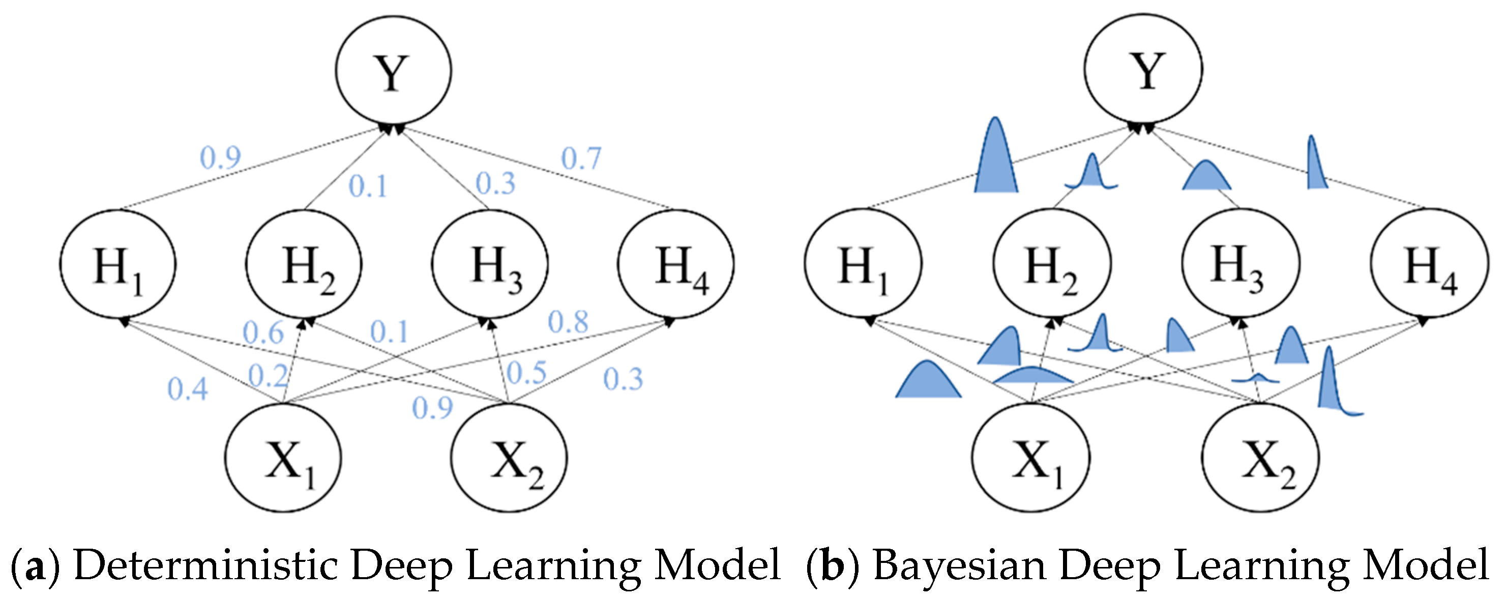
Traditional deterministic deep learning fits the mapping relationship between input and output data by optimizing weights and bias parameters, while Bayesian deep learning uses Bayesian inference methods to approximate the posterior distribution of model parameters rather than point estimation. Its core objective is to output a multi-step trajectory distribution that can simultaneously capture temporal evolution, spatial correlation, and predictive uncertainty. Figure 2 shows a schematic diagram of the comparison between deterministic and Bayesian deep learning models.

3.3.1. Bayesian Inference

The following subsections provide a brief overview of standard Bayesian deep learning techniques, including Bayesian inference, variational inference, KL divergence, and Monte Carlo sampling. These concepts are well established in the literature and are presented here only to support the description of our proposed BST-Transformer framework.

Bayesian inference is the specific application of Bayes’ theorem in the update of probability distributions. From a Bayesian perspective, the model parameters are treated as random variables with a posterior distribution defined by Bayes’ theorem. Its core idea is to use observed data to refine the prior distribution of unknown parameters, thereby obtaining the posterior distribution. Given an input sequence $X=\left\{x_1,\dots ,x_n\right\}$ and its corresponding output sequence $Y=\left\{y_1,\dots ,y_n\right\}$, the objective is to approximate the posterior distribution of network weights ω such that the function y = f^ω(x) best fits the training data. According to Bayes’ theorem, assuming a prior distribution $p\left(\omega \right)$ over the parameters ω, the posterior distribution can be computed as follows:

$$p\left(\omega \left|X,Y\right.\right)={\displaystyle \frac{p\left(Y\left|X,\omega \right.\right)\cdot p\left(\omega \right)}{p\left(Y\left|X\right.\right)}}$$

(9)

$p\left(\omega \left|X,Y\right.\right)$ is the posterior distribution of parameters given data, $p\left(Y\left|X,\omega \right.\right)$ is the likelihood, denoting the probability of observing $Y$ given $X$ and $\omega$, and $p\left(Y\left|X\right.\right)$ is the marginal likelihood, computed by integrating over all possible parameter values. Since the marginal likelihood is constant with respect to $\omega$, it is often treated as a normalization factor during inference.

After obtaining the posterior distribution $p\left(\omega \left|X,Y\right.\right)$ by combining the prior distribution and the likelihood function, the predictive distribution y* for a new input sample x* can be expressed as follows:

$$p\left(y^{\ast }\left|x^{\ast }\right.,X,Y\right)={\displaystyle \int p\left(y^{\ast }\left|x^{\ast }\right.,\omega \right)p\left(\omega \left|X,Y\right.\right)d\omega }$$

(10)

$p\left(y^{\ast }\left|x^{\ast }\right.,X,Y\right)$ represents the predictive probability distribution of the output.

This modeling framework can not only provide predictive estimation but also quantify uncertainty through the output distribution. It enables the model to capture temporal evolution, spatial dependence, and inherent uncertainties in the prediction process, which is crucial for downstream risk cognition and conflict assessment. However, the predictive distribution is obtained by marginalizing over the posterior (Equation (10)), which is intractable in closed form. Therefore, we need a more explicit approach to solve this problem.

3.3.2. Variational Inference

In practical applications, due to the high-dimensionality and nonlinear characteristics of deep neural networks and their activation functions, it is often difficult to directly calculate the precise posterior distribution $p\left(\omega \left|X,Y\right.\right)$. To solve this difficult problem, variational inference (VI) is often used to approximate the posterior distribution. The core idea is to introduce a simpler, tractable distribution $q_{\theta }\left(\omega \right)$ to approximate the true posterior $p\left(\omega \left|X,Y\right.\right)$ and iteratively optimize $q_{\theta }\left(\omega \right)$ during the training process to make it as close as possible to the true posterior. A common assumption is that $q_{\theta }\left(\omega \right)$ belongs to the Gaussian family, as shown in Equation (11):

$$Q_{\theta }\left(\mathsf{\Omega }\right)\sim N\left(\mu ,diag\left({\sigma }_d^2\right)\right)$$

(11)

In physics, the mean field theory is often employed to analyze systems with a large number of interacting components [48]. Similarly, in variational inference, the variational distribution is also decomposed under the mean field approximation:

$$Q_{\theta }\left(\mathsf{\Omega }\right)=\left\{q|q_{\theta }\left(\omega \right)={\displaystyle \prod _{i=1}^n{q}_{{\theta }_i}\left({\omega }_i\right)}\right\}$$

(12)

To measure the similarity between the true posterior distribution $p\left(\omega \left|X,Y\right.\right)$ and the variational approximation $q_{\theta }\left(\omega \right)$, the Kullback–Leibler (KL) divergence is used as the objective metric:

$$\begin{array}{cc}\hfill \underset{q_{\theta }\left(\omega \right)}{\min }KL\left(q_{\theta }\left(\omega \right)\left|\right|p\left(\omega |X,Y\right)\right)& ={\displaystyle \int q_{\theta }\left(\omega \right)\log \frac{q_{\theta }\left(\omega \right)}{p\left(\omega |X,Y\right)}}d\omega \hfill \\ & =KL\left(q_{\theta }\left(\omega \right)\left|\right|p\left(\omega \right)\right)+{\displaystyle \int q_{\theta }\left(\omega \right)\log \frac{q_{\theta }\left(Y|X\right)}{p\left(Y|X,\omega \right)}}d\omega \hfill \\ & =KL\left(q_{\theta }\left(\omega \right)\left|\right|p\left(\omega \right)\right)+\log p\left(Y|X\right)-{\displaystyle \int q_{\theta }\left(\omega \right)\log p\left(Y|X,\omega \right)}d\omega \end{array}$$

(13)

Since the marginal likelihood $p\left(Y|X\right)$ is constant with respect to $\omega$, minimizing the KL divergence is equivalent to maximizing the Evidence Lower Bound (ELBO) with respect to the variational parameters $\theta$, which balances data fit and regularization. The goal is to find the optimal variational parameters $\theta$ such that $q_{\theta }\left(\omega \right)$ closely approximates the true posterior while maintaining similarity to the prior $P\left(\omega \right)$. The ELBO is given by the following:

$$\begin{array}{cc}\hfill \underset{q_{\theta }\left(\omega \right)}{\max }ELBO\left(\theta \right)& ={\displaystyle \int q_{\theta }\left(\omega \right)\log p\left(Y|X,\omega \right)d\omega -KL\left(q_{\theta }\left(\omega \right)\left|\right|p\left(\omega \right)\right)}\hfill \\ & ={\displaystyle \int q_{\theta }\left(\omega \right)\log p\left(Y|X,\omega \right)d\omega -{\displaystyle \int q_{\theta }\left(\omega \right)\log \frac{q_{\theta }\left(\omega \right)}{p\left(\omega \right)}}}d\omega \hfill \\ & =E_{q_{\theta }\left(\omega \right)}\left[\log p\left(Y|X,\omega \right)\right]-E_{q_{\theta }\left(\omega \right)}\left[\log q_{\theta }\left(\omega \right)\right]+E_{q_{\theta }\left(\omega \right)}\left[\log p\left(\omega \right)\right]\hfill \\ & \approx {\displaystyle \frac{1}{N}}{\displaystyle {\sum }_{i+1}^N\left[\log p\left(Y|X,{\omega }_i\right)-\log q_{\theta }\left({\omega }_i\right)+\log p\left({\omega }_i\right)\right]}\hfill \end{array}$$

(14)

Equation (14) presents the Evidence Lower Bound (ELBO), the optimization objective for variational inference. The first term maximizes the expected log-likelihood under the approximate posterior, while the second term minimizes the divergence from the prior. Optimizing ELBO balances model fit and regularization, ensuring both predictive accuracy and calibrated uncertainty. Specifically, the process involves randomly sampling $\omega$, optimizing the parameters via backpropagation, updating the variational distribution $q_{\theta }\left(\omega \right)$, and repeating this process iteratively until convergence.

In this case, weight perturbation refers to sampling the weights of a random network during the training process. The reparameterization trick (Equation (15)) enables efficient sampling while keeping the process differentiable:

$$\omega =\overline{\omega }+\Delta \omega$$

(15)

However, naive Gaussian perturbation may lead to high variance and unstable gradient estimates. To address this issue, Wen et al. [49] proposed the Flipout technique, which introduces pseudo-independent perturbations for each sample in a mini batch without additional computational cost. The Flipout formulation is shown in Equations (16) and (17):

$$△{\omega }_n=△\widehat{\omega }\otimes r_n{s}_n^T$$

(16)

$$\omega =\overline{\omega }+△{\omega }_n$$

(17)

Δω_n is the perturbation matrix applied to the weight layer, r and s are random vectors whose elements are independently sampled from $\{-1,+1\}$, and $△\widehat{\omega }$ is shared basic perturbation and $△\widehat{\omega }\sim q_{\theta }\left(\omega \right)$.

3.4. Probabilistic TMA Trajectory Prediction Framework

3.4.1. BST-Transformer

The BST-Transformer (Bayesian Spatio-Temporal Transformer) is developed to perform trajectory prediction pre-training. The goal of this phase is to create a model capable of accurately modeling the multi-step probabilistic distribution of future aircraft trajectories, simultaneously capturing their motion patterns and inherent uncertainties. The first stage of this framework is dedicated to constructing the trajectory predictor BST-Transformer based on Bayesian inference, aiming to efficiently integrate the quantification of trajectory uncertainty into the prediction process. This design not only enhances the prediction accuracy but also outputs future trajectory data with confidence intervals, thus ensuring seamless integration with the aircraft conflict early warning module of the second stage.

Given that the ST-Transformer model established in previous studies [10] has demonstrated precise deterministic prediction capabilities under terminal area conditions, the BST-Transformer adds probabilistic interpretation capabilities by introducing Bayesian inference technology. This model is also based on the attention mechanism architecture and consists of three core components: the encoder, decoder, and uncertainty output module.

(1) Encoder

This encoder retains the temporal attention module and the spatial attention module and can efficiently model the temporal and spatial dependencies between trajectories. By capturing key features, the encoder can learn the inherent laws of aircraft movement, thereby achieving precise trajectory prediction. During the encoding process, the input trajectory sequence—containing spatio-temporal data spanning multiple time steps and aircraft—is processed to generate an encoded representation rich in context information, which not only captures the dynamic changes in time but also presents the spatial positional relationships between aircraft.

(2) Decoder

The Bayesian decoder has the ability to quantify uncertainty. Its architecture is shown in Figure 3, consisting of a Bayesian layer and a fully connected layer. The Bayesian layer is a key link in modeling and quantifying uncertainty—through Bayesian inference, it can capture the probability distribution of network weights and reflect the inherent uncertainty in the data. The fully connected layer further transforms the Bayesian output to generate the final prediction result. This step ensures the smoothness and stability of the decoder output.

During the model initialization stage, the prior distribution of network weights is usually assumed to follow a Gaussian distribution (i.e., $p\left(\omega \right)=\mathcal{N}\left(0,I\right)$), while the bias term is regarded as a point estimate. During the training process, the variational inference method is used to approximate the difficult-to-handle true posterior distribution. The Kullback–Leibler (KL) divergence is used to quantify the difference between the approximate distribution $q_{\theta }\left(\omega \right)$ and the true posterior distribution $p\left(\omega \left|X,Y\right.\right)$ Equation (18) defines the overall training objective, which combines the prediction loss with a KL regularization term. The goal of model optimization is to minimize this difference through Bayesian backpropagation. The total loss function Loss integrates both the prediction error and the KL divergence term simultaneously:

$$Loss=MSE+\lambda \cdot KL\left(q_{\theta }\left(\omega \right)‖p\left(\omega \left|X,Y\right.\right)\right)$$

(18)

$\lambda$ is a weight coefficient used to control the contribution of the KL divergence term, $\lambda \in \left[0,1\right]$.

After obtaining the approximate posterior distribution through variational inference, the uncertainty output module performs Monte Carlo (MC) sampling by drawing N samples from $q_{\theta }\left(\omega \right)$, and then the expected approximate distribution of $y^{*}$ can be obtained; that is, the probability distribution of the final predicted trajectory points. Equation (19) shows the Monte Carlo approximation of the predictive distribution:

$$\begin{array}{l}p\left(y^{\ast }\left|x^{\ast }\right.,X,Y\right)=E_{p\left(\omega \left|X,Y\right.\right)}\left[p\left(y^{\ast }\left|x^{\ast }\right.,\omega \right)\right]\\ \approx {\displaystyle \frac{1}{N}}{\displaystyle \sum _{k=1}^{N}p\left(y^{\ast }\left|x^{\ast }\right.,{\widehat{\omega }}_k\right)}\end{array}$$

(19)

${\widehat{\omega }}_k$ is the weight matrix obtained for each sampling.

3.4.2. Aircraft Conflict Alerting Module

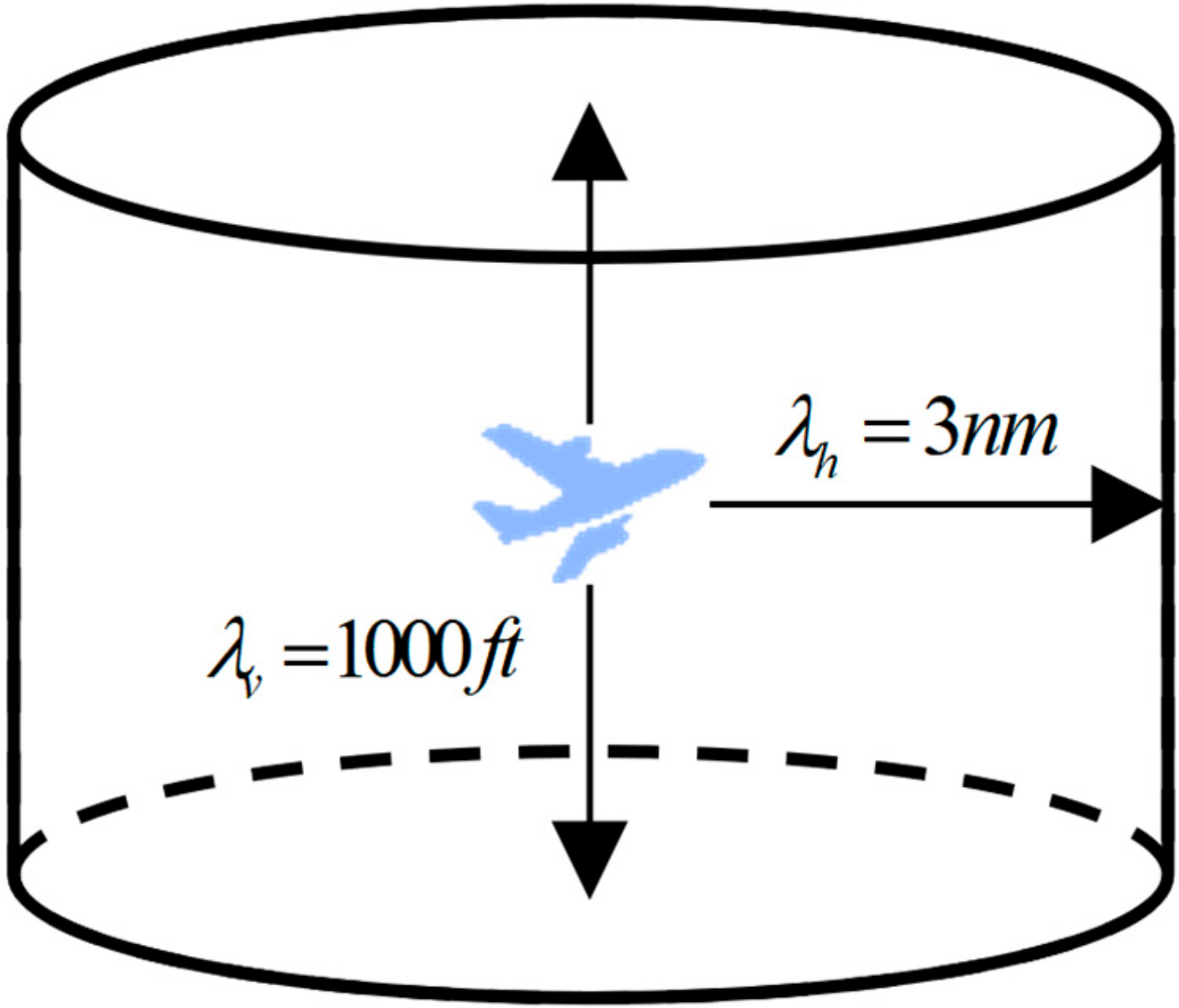
Safety is the cornerstone of the civil aviation industry. Although absolute safety is hard to achieve, it is necessary to maintain continuous and acceptable safety standards. Air traffic controllers are mainly responsible for managing air traffic flow and ensuring operational safety. When these two goals conflict, security must come first—even if it means sacrificing operational efficiency. As a core component of TBO, the aircraft conflict warning system continuously monitors and analyzes the real-time flight status of the aircraft. These systems can proactively identify potential conflicts and issue alerts, thereby assisting controllers in decision-making, reducing their workload, and enhancing safety and operational efficiency in complex airspace environments. According to the “Air Traffic Control Manual” of the Federal Aviation Administration (FAA) of the United States [50], the minimum interval standard for radar-guided operations in air traffic control areas is 3 nautical miles horizontally and 1000 feet vertically, as shown in Figure 4

In the deterministic conflict early warning model, the aircraft safety zone is pre-set through geometric shapes such as cylinders, spheres or ellipsoids. When one aircraft enters the protected area of another, the system will trigger conflict detection. In contrast, probabilistic conflict early warning models focus on the uncertainty of future flight trajectories. This model predicts the probability of a conflict between any two aircraft at some point in the future and triggers an alarm when the probability value exceeds the preset threshold. In the framework proposed in this study, the aircraft conflict early warning module in the second stage takes probabilistic trajectory prediction as input data to calculate the probability of paired conflicts. This design can achieve early warning of potential safety hazards.

Let aircraft $i$ and $j$ have predicted positions $L_i^t=\left(x_i^t,y_i^t,z_i^t\right)$ and $L_j^t=\left(x_j^t,y_j^t,z_j^t\right)$ at time $t$. A potential conflict is identified if either of the following conditions is met:

$$I\left[p\left(r_h\left(L_i^t,L_j^t\right)<{\lambda }_h\right)>{\delta }_h\mathrm{and}p\left(r_h\left(L_i^t,L_j^t\right)<{\lambda }_v\right)>{\delta }_v\right]$$

(20)

$r_h\left(L_i^t,L_j^t\right)$ and $r_v\left(L_i^t,L_j^t\right)$ are the horizontal and vertical separation distances of two aircrafts; ${\lambda }_h$ and ${\lambda }_v$ are minimum separation thresholds (3 nmNM and 1000 ft). $p\left(r_h\left(L_i^t,L_j^t\right)<{\lambda }_h\right)$ and $p\left(r_v\left(L_i^t,L_j^t\right)<{\lambda }_v\right)$ are predefined alert probability thresholds in each dimension. If the probability of conflict in either direction exceeds the corresponding threshold, an alarm will be issued, indicating a possible violation of the safety interval.

In practical computation, if the predicted trajectory points of aircraft i and j follow distributions $f_i^t\left(L_i^t\right)$ and $f_j^t\left(L_j^t\right)$ the conflict probability at time t can be expressed as follows:

$$P_{ij}^t={\displaystyle {\int }_{r\le \lambda }f\left(r\right)dr,r=‖f_i^t\left(L_i^t\right)-f_j^t\left(L_j^t\right)‖}$$

(21)

$f\left(r\right)$ represents the distance distribution function between two aircraft, and λ represents the minimum safe distance. To reflect the different safety margins in the horizontal and vertical directions, the overall conflict probability is further decomposed as fol-lows:

$$\begin{array}{l}{P}_{ij}^t={\displaystyle {\int }_{\begin{array}{l}\sqrt{△x^2+△y^2}\le {\lambda }_h\\ \left|△z\right|\le {\lambda }_v\end{array}}f\left(△x,△y,△z\right)d△xd△yd△z}\\ △x=\left|x_i^t-x_j^t\right|,△y=\left|y_i^t-y_j^t\right|,△z=\left|z_i^t-z_j^t\right|\end{array}$$

(22)

This requires the integration calculation of the joint distance distribution within the area defined by the safety threshold.

Given the infeasibility of the analysis of this integral, we adopted the Monte Carlo simulation method. At each time step t, $N$ samples are drawn from the predicted trajectory distributions of aircraft $i$ and $j$. For each sample $L_i^t$ and $L_j^t$, the horizontal and vertical distances are calculated. If $N_{conflict}$ out of $N$ sample pairs violate the minimum separation, Equation (23) estimates the conflict probability between aircraft $i$ and $j$ at time $t$.

$$P_{ij}^t{\displaystyle \frac{N_{conflict}}{N}}$$

(23)

4. Experiments

4.1. Datasets

The trajectory data adopted in this study is derived from the secondary surveillance radar (SSR) system deployed in the air traffic control infrastructure. By regularly examining the aircraft transponder, the SSR system can obtain key information such as the aircraft’s position, altitude, and speed. Compared with the ADS-B (Automatic Correlation Surveillance Broadcast) data commonly used in recent studies, SSR data has a higher sampling frequency and a lower data loss rate, and it is particularly suitable for multi-target trajectory prediction and conflict probability assessment research in high-density air traffic control areas.

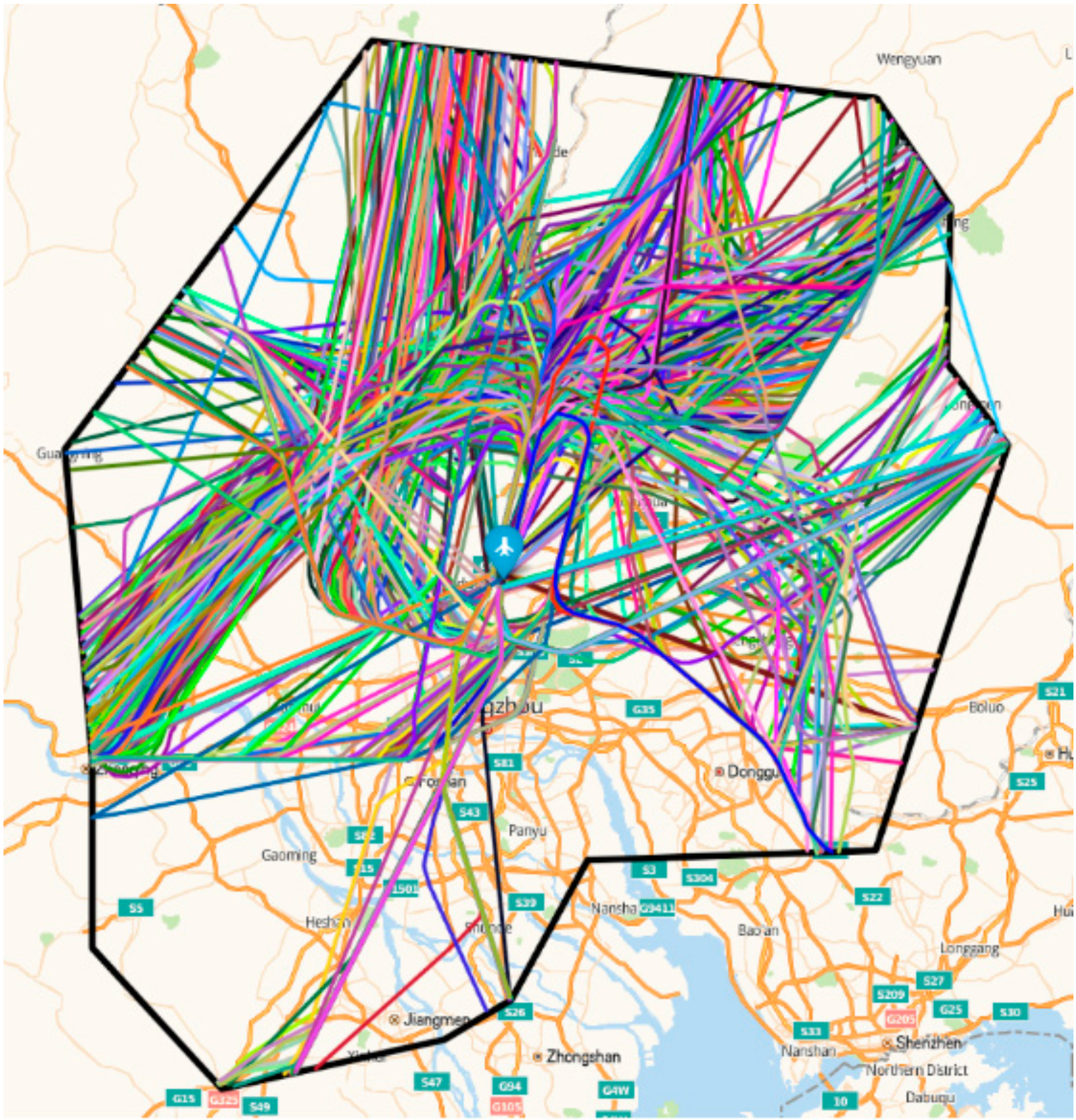
To support the modeling of trajectory distribution and uncertainty in the air traffic control area, we selected the radar trajectory data of a busy operating day in the Guangzhou Air Traffic Control Area (TMA)—this area typically reflects the characteristics of a complex operating environment. The selected area features typical scenarios such as complex airspace structure, large passenger flow, and the convergence of multiple airport air traffic control zones, providing a highly representative research example for simulating actual operational pressure and predicting challenges. Figure 5 shows the original trajectory of Guangzhou TMA.

The original radar data is stored in format $\left(la{t}_i^t,lo{n}_i^t,al{t}_i^t\right)$, and these data cannot be directly used to calculate spatial distances or relative orientations during the modeling process. For this purpose, we take the center of the main runway of Guangzhou Baiyun International Airport as the coordinate origin and use Mercator projection to convert all trajectory points to the two-dimensional 8Cartesian coordinate system $\left(X_i^t,Y_i^t,Z_i^t\right)$. Before the model is input, the data is optimized through preprocessing steps such as deduplication, missing value analysis, and time series resampling.

(1)

Time resampling is carried out with a fixed step of 5 s. If the trajectory point is missing, fill it by linear interpolation between adjacent time steps.

$$X_i^t=X_i^{t-1}+{\displaystyle \frac{X_i^{t+1}-X_i^{t-1}}{\left(t+1\right)-\left(t-1\right)}}\left(t-\left(t-1\right)\right)$$

(24)

(2)

Perform linear interpolation correction on the trajectory points with incomplete positions.

(3)

Convert the timestamp into a relative time difference and label the flight ID to ensure the consistency of the input features.

(4)

To meet the requirement of Bayesian network modeling for complete trajectory observation, only complete trajectory fragments covering the entire takeoff or landing stage were selected.

Thus, the feature vector for the i aircraft at time t can be defined as follows:

$$X_i^t=\left[t_i,c{s}_i,la{t}_i^t,lo{n}_i^t,al{t}_i^t\right]$$

(25)

$t_i$ is the timestamp (relative to a base time), $c{s}_i$ is the label-encoded flight identifier, and $la{t}_i^t$, $lo{n}_i^t$, $al{t}_i^t$ represent the latitude, longitude, and altitude of the aircraft $i$ at time $t$, respectively. This preprocessing guarantees that all input dimensions share compatible units and scales, which facilitates stable model training and evaluation.

To facilitate the precise calculation of aircraft spacing, the Mercator projection with the center point of the airport runway as the projection origin is adopted. The conversion process from the geodetic coordinate system to Cartesian coordinates is as follows:

$$\left\{\begin{array}{l}k={\displaystyle \frac{a^2}{b\sqrt{1+{e^{\prime }}^2{\cos }^2\left(la{t}_0\right)}}}\cos \left(la{t}_0\right)\\ x=k\left(lon-lo{n}_0\right)\\ y=k\ln \left(\tan \left({\displaystyle \frac{\pi }{4}}+{\displaystyle \frac{lat}{2}}\right)\times {\left({\displaystyle \frac{1-e\sin lat}{1+e\sin lat}}\right)}^{{\displaystyle \frac{e}{2}}}\right)\end{array}\right.$$

(26)

$\left(x,y\right)$ are the projected Cartesian coordinates, $\left(lon,lat\right)$ are the original coordinates, $\left(lo{n}_0,la{t}_0\right)$ are the geodetic coordinates, taking the intersection point of 0° latitude and 0° longitude as the projection reference point, the semi-major axis of the Earth $a$ is set to 6,378,137 m, and the semi-minor axis $b$ is set to 6,356,752 m. The first eccentricity $e$ is set to 0.0818, and the second eccentricity $e^{\prime }$ is set to 0.0821. Based on this, the projected coordinate of the origin point $\left(x_0,y_0\right)$ can be obtained. Then, the projected coordinate $\left(x_i,y_i\right)$ of any trajectory point converted from its original latitude and longitude can be further transformed into its actual Cartesian coordinate $\left(x,y\right)$ representation.

$$\left\{\begin{array}{l}x=x_i-x_0\\ y=y_i-y_0\end{array}\right.$$

(27)

Ultimately, we retained 1211 complete flight trajectories for model training. All flight trajectories take off and land at Guangzhou Baiyun International Airport, covering several hours of high-density operation periods. The average trajectory duration is between 4 and 8 min, which makes the dataset highly suitable for multi-step probability prediction.

It should be particularly noted that although this dataset partially overlaps with the data sources used in some existing literature, this study has significant differences in research objectives, modeling strategies, and application directions. Specifically, this study focuses on distributed trajectory prediction and conflict probability reasoning, emphasizing the quantification of uncertainties and their integration into intelligent early warning systems—which is fundamentally different from traditional point-by-regression tasks.

4.2. Evaluation Metrics

Since the longitude and latitude data have been converted into a Cartesian coordinate system centered on the airport during the data preprocessing stage, we use the following indicators to evaluate the trajectory prediction performance: mean absolute displacement error (MADE), mean absolute displacement horizontal error (MADHE), and mean absolute displacement vertical error (MADVE). All indicators are in meters. The corresponding formulas are as follows: DE represents the three-dimensional Euclidean distance between the predicted trajectory point and the actual trajectory point, DHE refers to the horizontal two-dimensional distance within the plane, and DVE represents the height difference between the predicted value and the actual value. The smaller the values of these error indicators are, the better the predictive performance of the model on the given dataset is.

$$MADE={\displaystyle \frac{{\displaystyle \sum _{i=1}^N{\displaystyle \sum _{t=1}^{T_{pred}}\sqrt{{\left(X_i^t-{\widehat{X}}_i^t\right)}^2+{\left(Y_i^t-{\widehat{Y}}_i^t\right)}^2+{\left(Z_i^t-{\widehat{Z}}_i^t\right)}^2}}}}{N\left(T_{pred}-1\right)}}$$

(28)

$$MADHE={\displaystyle \frac{{\displaystyle \sum _{i=1}^N{\displaystyle \sum _{t=1}^{T_{pred}}\sqrt{{\left(X_i^t-{\widehat{X}}_i^t\right)}^2+{\left(Y_i^t-{\widehat{Y}}_i^t\right)}^2}}}}{N\left(T_{pred}-1\right)}}$$

(29)

$$MADVE={\displaystyle \frac{{\displaystyle \sum _{i=1}^N{\displaystyle \sum _{t=1}^{T_{pred}}\sqrt{{\left(Z_i^t-{\widehat{Z}}_i^t\right)}^2}}}}{N\left(T_{pred}-1\right)}}$$

(30)

$\left(X_i^t,Y_i^t,Z_i^t\right)$ denotes the true three-dimensional trajectory coordinate of aircraft $i$ at time $t$, $\left({\widehat{X}}_i^t,{\widehat{Y}}_i^t,{\widehat{Z}}_i^t\right)$ denotes the predicted three-dimensional coordinate at the same time, N is the total number of aircraft, and $T_{pred}$ is the prediction sequence length.

4.3. Trajectory Prediction Results Analysis

To evaluate the proposed Bayesian trajectory prediction framework, we designed a training process specifically for probabilistic modeling tasks. In the first stage, we verified the performance of the BST-Transformer predictor using the differentiable variational inference structure built based on Python 3.10 with PyTorch 2.1.0. The training objective is to maximize the Evidence Lower Bound (ELBO), which consists of two components: (1) reconstruction loss, which measures the fit between the predicted trajectory distribution and the observed trajectory through a negative log-likelihood function; (2) for the regularization term, the Kullback–Leibler (KL) divergence measure is adopted to ensure that the learned posterior distribution is close to the assumed prior distribution, thereby enhancing the generalization ability of the model.

Considering the high spatiotemporal complexity of trajectory prediction and the known challenges such as unstable gradients and slow convergence in the early training of Bayesian models, we additionally adopted the mean square error (MSE) as an auxiliary evaluation metric in the initial training stage. MSE is used to measure the deviation between the predicted mean trajectory and the true value and can provide diagnostic feedback for systematic deviation. Although MSE is not included in the final loss function, it serves as an external signal to assist in model tuning and is used to detect overfitting/underfitting phenomena.

In the process of predictive modeling, the rational selection of hyperparameters plays a critical role in model performance. Optimizing the selection of hyperparameters can strike a balance between the model’s fitting ability and generalization ability, thereby enhancing the accuracy and stability of trajectory prediction results. The parameters of the BST-Transformer model fall into two categories: one is the network weight parameters, namely the weights and bias terms of neuron connections. Their initial values are generated through random initialization and are automatically updated during the training process using the stochastic gradient descent method to minimize the loss function; an-other category is hyperparameters, which involve both model structure design and training strategies. By pre-setting the search range of hyperparameters and combining different values, multiple candidate configurations can be obtained, thereby screening out the parameter scheme that can optimize the loss function. The dataset is divided into 80% training sets and 20% test sets. Each training iteration uses the Adam optimizer, with an initial learning rate of 0.0015 and a batch size of 128. This model adopts a double-layer Transformer encoder architecture, equipped with eight attention heads, with a hidden layer dimension of 32 and a dropout rate of 0.05. Weight perturbation is carried out through the Flipout mechanism to enhance the model’s perception ability of parameter uncertainty. The training process is set with a maximum of 100 iterations. After each round of training, the convergence of the ELBO is monitored to preserve the optimal model weights for the inference and early warning tasks. The model hyperparameters are set as

Table 1. Model hyperparameters.

Parameter	Parameter Value
num of heads	8
num of encoder layers	2
dimension of model	32
dropout	0.05
learning rate	0.0015
train epoch	100
num of aircraft stored as one batch	128

. Model hyperparameters.

To thoroughly evaluate the performance of the proposed BST-Transformer, we compare it against several representative baseline methods in trajectory prediction. The baseline implementations (BP, RNN, LSTM, SR-LSTM, and ST-Transformer) follow the configurations described in our previous work [10], where these models were systematically evaluated on the same trajectory dataset. In this study, they are included again to provide a fair comparison framework and to highlight the improvements achieved by the proposed BST-Transformer. For all models, the batch size is set to 7, with each batch containing around 128 aircraft from different time windows. The activation function used is ReLU, and the Adam optimizer is employed. The comparison model and its parameter settings are as follows:

(1)

Back Propagation (BP) Neural Network: A classic multi-layer feedforward network trained with the backpropagation algorithm, which serves as a fundamental nonlinear function approximator benchmark. The embedding size is set to 32, the number of neurons per hidden layer is 64, the dropout rate is 0.1, the learning rate is 0.0019, and the number of training epochs is 200.

(2)

Recurrent Neural Network (RNN): A fundamental neural network architecture designed for sequential data, which utilizes cyclic connections to maintain a hidden state that captures historical information. The loss function converged within 100 training epochs and the number of epochs is 100. The embedding size is 32, number of hidden layers is 2, number of neurons per hidden layer is 64, dropout rate is 0.1, and learning rate is 0.0015.

(3)

Long Short-Term Memory (LSTM): An advanced variant of RNN that introduces gating mechanisms to mitigate the vanishing gradient problem and better capture long-range dependencies. The loss function converged within 100 training epochs and the number of epochs is set to 100. The embedding size is 32, number of hidden layers is 2, number of neurons per hidden layer is 64, dropout rate is 0.1, and learning rate is 0.0015.

(4)

State Refined LSTM (SR-LSTM): An extension of LSTM that explicitly models the interaction between different temporal states of a single sequence through a state refinement module, enhancing its ability to capture complex temporal patterns. The loss function converged within 100 training epochs and the number of epochs is set to 100. The number of refinement layers is set to 2.

(5)

ST-Transformer: The deterministic version of the Spatio-Transformer, which shares the same spatio-temporal attention architecture as our model but without Bayesian uncertainty quantification. This comparison is crucial to isolate the benefit of our Bayesian framework [10]. The training epochs are 100.

(6)

ST-Transformer Dropout: The Dropout model of the ST-Transformer approximates the Bayesian inference process by applying Dropout to simulate the posterior distribution. This method is based on the equivalence between Monte Carlo Dropout and ELBO maximization, a principle that has been confirmed by the research of Gal et al. [51].

All models were trained using the same trajectory dataset and the same training and testing split ratio. The aim is to analyze the strengths and weaknesses of each model in trajectory prediction through horizontal comparison.

Table 2. Error evaluation metrics.

Model	MADE (m)	MADHE (m)	MADVE (m)
BP	5841.98	5834.31	242.60
RNN	3060.21	3041.44	243.91
LSTM	2616.54	2593.01	237.53
SR-LSTM	2608.83	2583.24	233.36
ST-Transformer	1365.27	1353.54	100.53
ST-Transformer Dropout	703.45	688.78	77.25
BST-Transformer	542.37	511.98	52.36

summarizes the error indicators of each model. For probabilistic models, their error values are obtained by averaging 20 trajectory samples and comparing them with the true values.

The experimental results show that the proposed probability model is superior to the deterministic model in terms of prediction accuracy. The BST-Transformer achieves superior uncertainty modeling through the weight perturbation technique based on Flipout. Compared with the standard Dropout method, this technique not only retains the neuron structure but also provides a more expressive modeling effect.

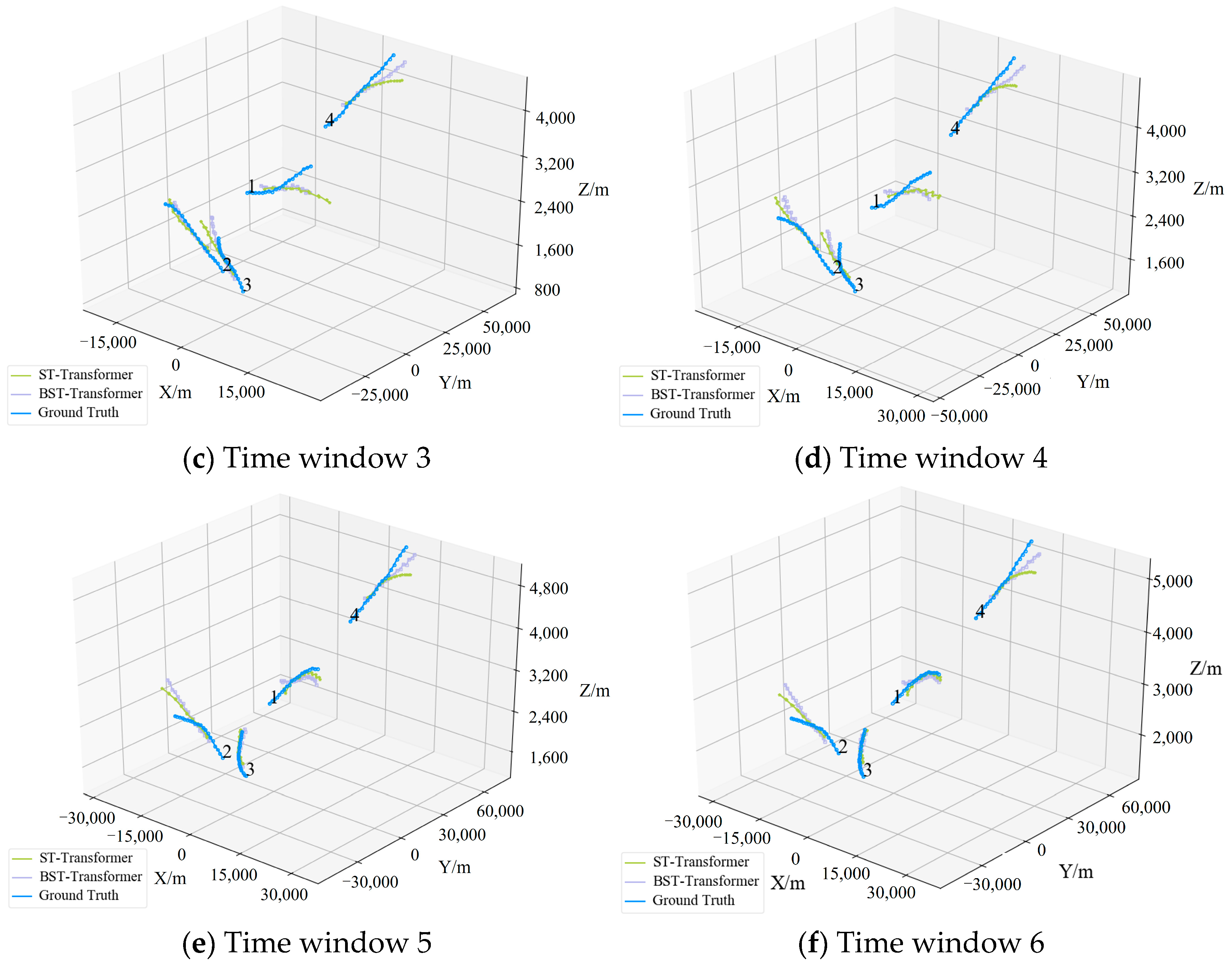
To visually compare the BST-Transformer with the deterministic baseline model, we conducted three-dimensional trajectory prediction visualization for the four aircraft involved in the spatial structure diagram (see Figure 6). The results show that the multi-step cumulative error of the BST-Transformer is significantly reduced, fully demonstrating its robustness in the complex airway airspace environment.

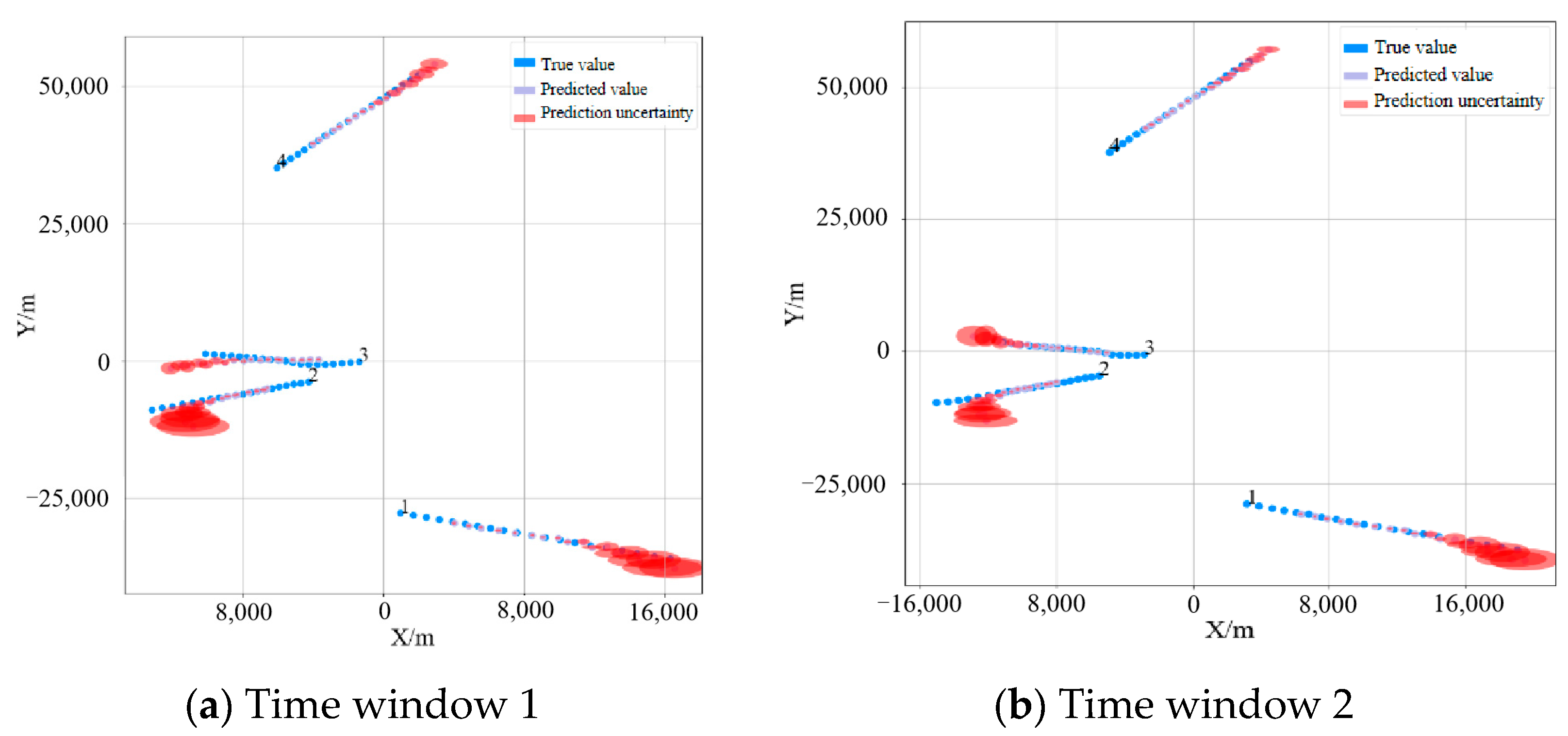
We further demonstrate the uncertainty of the prediction through a two-dimensional graph (Figure 7). The blue line represents the true value, the purple line represents the predicted mean, and the red area represents the 95% confidence interval. Due to their close spatial positions and being in an active maneuvering state (such as turning), Aircraft 2 and 3 exhibit considerable uncertainty. Aircraft 1 and 4, on the other hand, exhibit more stable flight modes with lower uncertainty. Most of the prediction confidence intervals cover the true values, which indicates that the quantitative effect of uncertainty is significant.

Figure 8 shows the standard deviations of altitude predictions within six time windows. The left side of each chart represents the observation timestamp, while the right side shows the future predicted value. As expected, the uncertainty of prediction increases with the extension of the prediction time range. Aircraft 2 and 3 once again exhibit a high standard deviation, which is consistent with the spatial interaction observed in the previous chart.

The Bayesian training introduces additional training overhead compared with the deterministic ST-Transformer; in our hardware environment (Intel Xeon Gold 6330 CPU + NVIDIA RTX 3090 GPU) we estimate that typical training for 100 epochs on the 1211-flight dataset will be on the order of 1 h for the deterministic model and about 1.5–2 h for the Bayesian model, depending on implementation details and sequence length.

4.4. Conflict Alert Analysis

After completing the accuracy verification and probability output validation of the BST-Transformer algorithm, we set out to evaluate the performance of its second-stage conflict early warning module. The selected case study is drawn from real SSR data in the Guangzhou TMA. Guangzhou Baiyun International Airport operates multiple parallel runways, which is relevant for interpreting crossing geometries. The example involving CBJ5270 and CES9767 represents a typical high-density encounter where horizontal trajectories intersect but vertical separation and runway assignments prevent an actual conflict. This case was chosen as it illustrates how the Bayesian framework provides a probabilistic assessment that distinguishes between apparent crossings and genuine risks. Taking the approach data of flights CBJ5270 and CES9767 at Guangzhou Baiyun Airport as the research case, we found that these flight paths frequently crossed trajectories in the horizontal and vertical directions, especially in the final approach stage. This phenomenon not only highlights the potential risk of conflict but also emphasizes the necessity of strengthening trajectory monitoring.

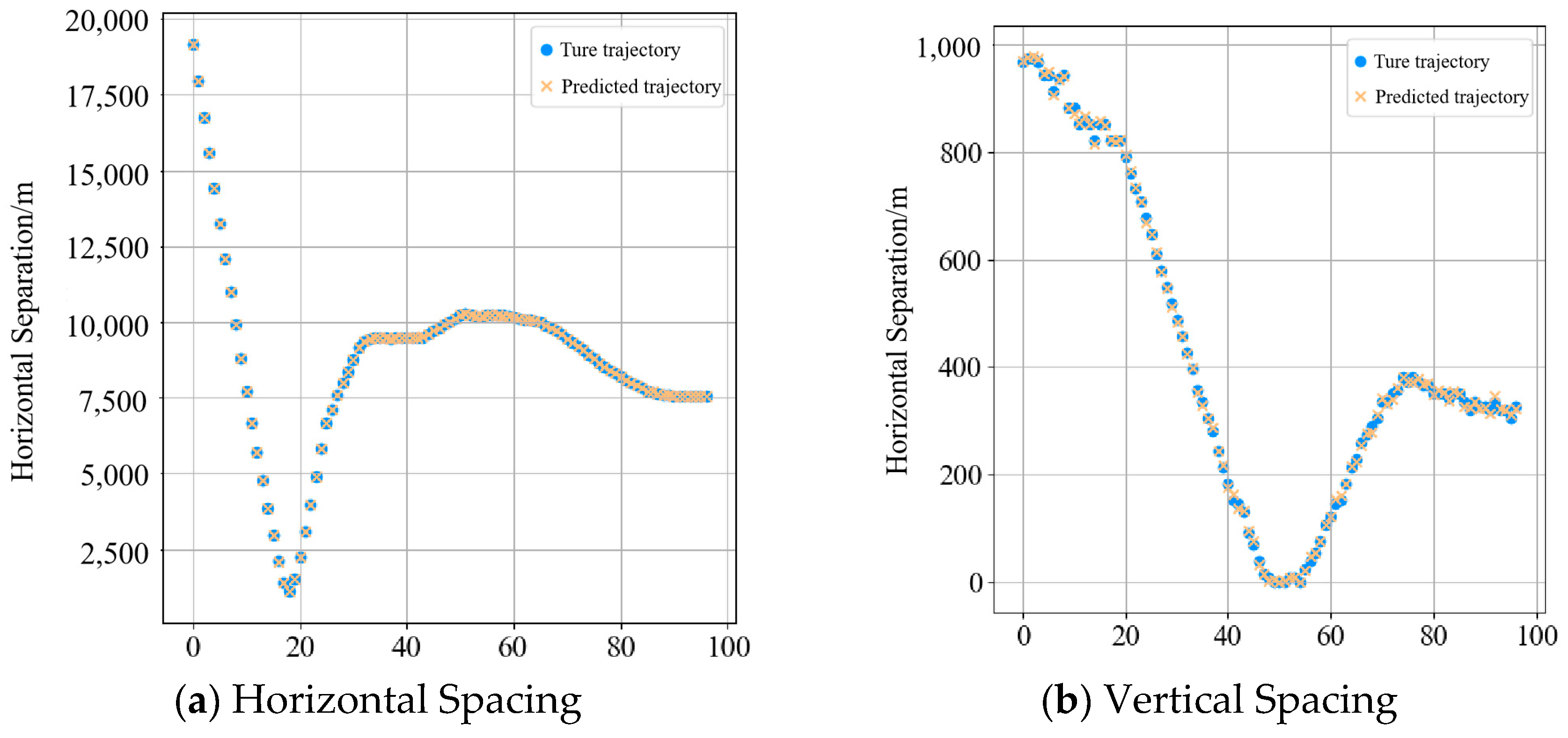
Figure 9 illustrates the relative horizontal trajectories of aircraft CBJ5270 and CES9767 within the Guangzhou TMA. Although the trajectories intersect laterally, the aircraft maintain vertical separation because they are assigned to different runways. This crossing geometry highlights a typical scenario where horizontal proximity does not necessarily indicate a true loss of separation, emphasizing the need for probabilistic conflict assessment rather than purely deterministic distance checks.

We used predicted trajectories to calculate the spatial distance between aircraft and extracted the critical approach interval (Figure 10). The prediction results of the BST-Transformer model are highly consistent with the real spatial trend, which verifies the reliability of the model in the assessment of conflict probability.

To evaluate the distribution characteristics of the predicted trajectories, we used Monte Carlo simulation to draw 5000 samples from the posterior distribution. Figure 11 shows the frequency histograms of the sampling trajectory points in the x, y, and z dimensions. The results show that the data approximately follow a normal distribution centered on the predicted mean. The normality of the distribution was verified through the Anderson–Darling test, which provided strong support for the effectiveness of sampling-based methods.

For probabilistic conflict estimation, Monte Carlo sampling (M = 5000) provides robust probability estimates but increases inference time: a conservative estimate for a single pairwise probability computation is tens of seconds to a few minutes, although efficient GPU batching and parallelization can bring this down significantly (e.g., to the order of 10–100 s per pair in typical settings). Therefore, ensuring real-time feasibility in dense TMAs requires additional engineering, which we identify as future work.

Subsequently, we calculate the conflict probability based on the sampled trajectory data at intervals of 5 s.

To further quantify the effectiveness of the probabilistic conflict alerting framework, Receiver Operating Characteristic (ROC) and Precision–Recall (PR) curves were constructed based on the predicted conflict probabilities across 200 timestamps(Figure 12). The ROC curve illustrates the trade-off between the true positive rate (detection rate) and the false positive rate at different probability thresholds, while the PR curve reflects the balance between precision and recall under class imbalance. Both curves demonstrate strong discriminative performance, with AUC values of 0.9 (ROC) and 0.87 (PR), indicating that the proposed model can reliably distinguish conflict from non-conflict situations.

When examining the operational thresholds adopted in this study, the results are consistent with the ROC/PR analysis. At a probability threshold of 0.6, the model achieves a higher detection rate but at the cost of increased false alarms, which may be preferable in safety-critical contexts where missing a conflict is unacceptable. At the more conservative threshold of 0.8, the false alarm rate is significantly reduced, but some potential conflicts are detected later, reflecting a trade-off between sensitivity and alert stability. These findings confirm that the chosen thresholds (0.6 and 0.8) represent meaningful operating points within the probabilistic framework and provide flexibility for controllers to balance safety and workload in different traffic conditions.

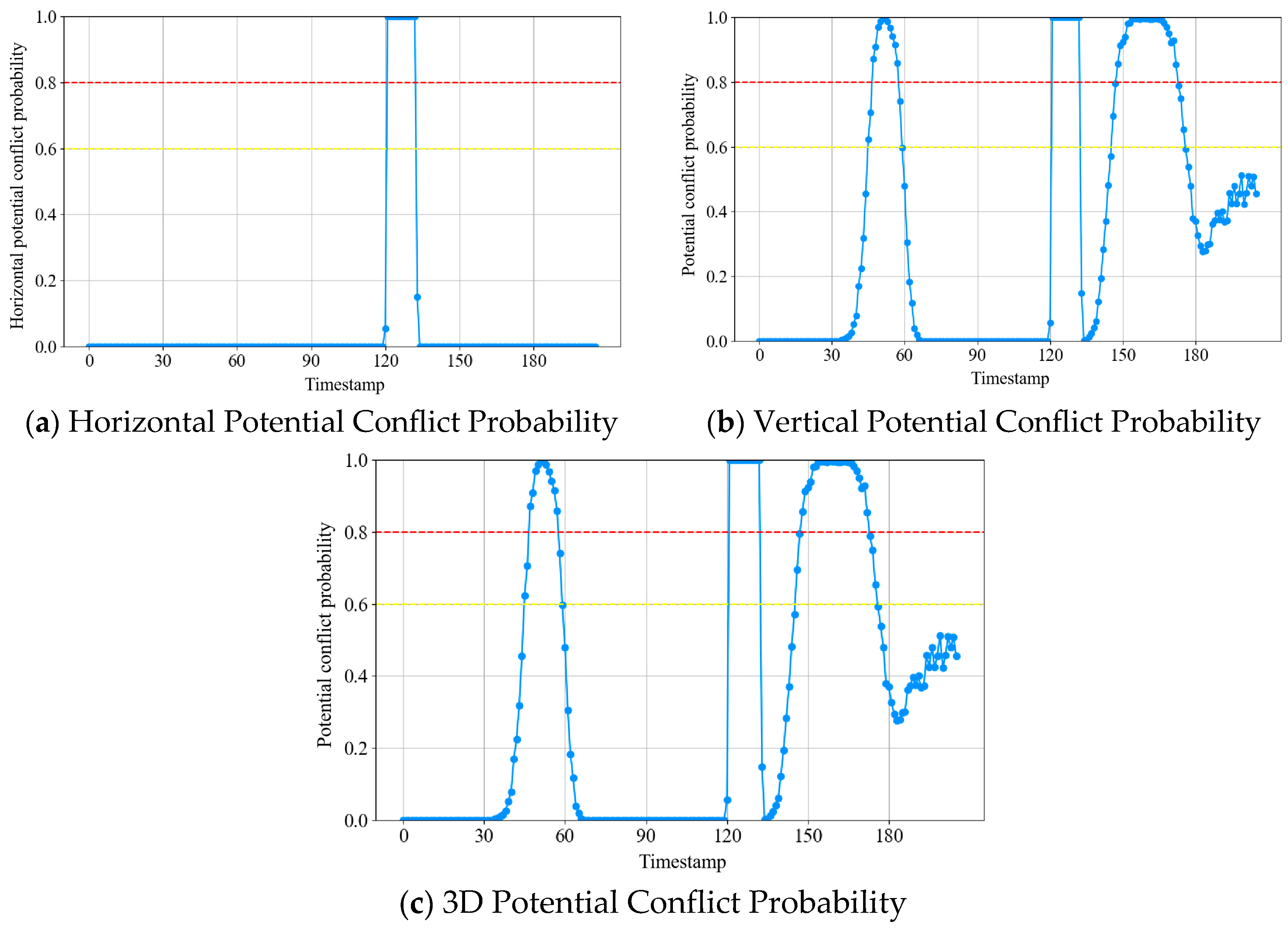
Figure 13 shows the analysis results in the horizontal, vertical, and three-dimensional spatial directions. The three-dimensional conflict probability graph (Figure 13c) shows that a total of 56 warning points were detected at the 0.6 threshold, while there were 48 warning points at the stricter 0.8 threshold. Note on threshold lines in Figure 13. In Figure 13, the two horizontal dashed lines correspond to the alert probability thresholds used in our case study: 0.6 (moderate alert) and 0.8 (high alert). A conflict is considered to be flagged at time t when the estimated conflict probability exceeds the chosen threshold. We emphasize these values are illustrative rather than operational standards. In practice, threshold values should be calibrated in consultation with ATC operational requirements and risk tolerances.

The conflict probability was computed via Monte Carlo sampling with 5000 draws. On our experimental hardware, the average inference time per trajectory sequence was ~0.15s, and the entire sampling process required only a few seconds, demonstrating feasibility for offline evaluation. However, in dense TMA scenarios, scalability may become critical as the number of aircraft pairs increases quadratically. Preliminary tests suggest that reducing the sample size to 1000 yields only a marginal change in probability estimation (2% deviation in peak probability), while significantly lowering runtime. This indicates that adaptive or dynamic sampling strategies could provide a practical trade-off between computational efficiency and prediction accuracy.

5. Conclusions

Trajectory prediction and conflict detection in TMA remain critical challenges in air traffic management. To address these challenges, this paper proposes a Bayesian spatio-temporal deep learning framework (BST-Transformer) that integrates temporal and spatial attention mechanisms for probabilistic trajectory prediction and conflict alerting. Unlike deterministic models, the proposed framework explicitly quantifies predictive uncertainty and incorporates it into the conflict alerting process through Monte Carlo sampling. This probabilistic design enables the estimation of conflict probability distributions rather than binary outcomes, thereby providing a more reliable foundation for operational decision-making.

The main innovations of this study are threefold. First, the BST-Transformer extends the deterministic ST-Transformer by embedding Bayesian inference, allowing uncertainty-aware trajectory forecasting in complex terminal environments. Second, a probabilistic conflict alerting module is developed, which directly connects trajectory distributions to conflict probability evaluation. Third, extensive experiments on real SSR data from the Guangzhou TMA demonstrate that the proposed approach significantly improves prediction accuracy and robustness compared with representative baselines, while offering interpretable conflict probability estimates for practical risk assessment.

The experimental results confirm that the Bayesian framework enhances both accuracy and reliability, though at the expense of increased computational cost. This highlights the trade-off between robustness and efficiency, especially in dense TMAs where scalability becomes critical. In the future, our research will extend in two directions. On the methodological side, we will explore adaptive sampling and lightweight Bayesian approximations to improve computational efficiency for real-time applications. On the application side, we will incorporate richer features such as heading, speed, aircraft type, and meteorological conditions to further enhance predictive performance. Finally, integration with decision-support systems and Trajectory Based Operations (TBO) modules will help translate the proposed method into practical tools for intelligent air traffic control.

References

1. International Air Transport Association. World Air Transport Statistics; IATA: Montreal, QC, Canada, 2023; Available online: https://www.iata.org (accessed on 14 March 2024).
2. IATA. World Air Transport Statistics (WATS), 2024 ed.; International Air Transport Association (IATA): Montreal, QC, Canada, 2024; Available online: https://www.iata.org/en/services/data/market-data/world-air-transport-statistics/ (accessed on 7 June 2025).
3. Performance Review Commission (PRC), EUROCONTROL. Performance Review Report 2022: An Assessment of Air Traffic Management in Europe; Eurocontrol: Brussels, Belgium, 2023; Available online: https://www.eurocontrol.int/sites/default/files/2023-06/eurocontrol-prr-2022.pdf (accessed on 18 December 2024).
4. ICAO. Trajectory Based Operations (TBO)—Global Concept/Operational Guidance; International Civil Aviation Organization (ICAO): Montreal, QC, Canada, 2025; Available online: https://www2023.icao.int/airnavigation/tbo/Pages/Why-Global-TBO-Concept.aspx (accessed on 6 August 2025).
5. Guo, P.; Liang, B.; Li, S.; Yang, K.; Li, Q. Research on Trajectory Conflict Detection and Resolution for TBO. In Proceedings of the International Conference on Guidance, Navigation and Control, Changsha, China, 9–11 August 2024; Springer Nature: Singapore, 2024; pp. 381–392. [Google Scholar] [CrossRef]
6. FAA/EUROCONTROL. Common TP Structure and Terminology in Support of SESAR & NextGen; FAA/Eurocontrol: Brussels, Belgium, 2010.
7. Ma, L.; Tian, S. A Hybrid CNN-LSTM Model for Aircraft 4D Trajectory Prediction. IEEE Access 2020, 8, 134668–134680. [Google Scholar] [CrossRef]
8. Song, Y.; Cheng, P.; Mu, C. An Improved Trajectory Prediction Algorithm Based on Trajectory Data Mining for Air Traffic Management. In Proceedings of the 2012 IEEE International Conference on Information and Automation, Chengdu, China, 6–8 June 2012; IEEE: Shenyang, China, 2012; pp. 981–986. [Google Scholar] [CrossRef]
9. Chen, H.; Jilkov, V.P.; Li, X.R. On Threshold Optimization for Aircraft Conflict Detection. In Proceedings of the 18th International Conference on Information Fusion, Washington, DC, USA, 6–9 July 2015; IEEE: Washington, DC, USA, 2015; pp. 1198–1204. Available online: https://www.webofscience.com/wos/alldb/full-record/WOS:000389523300157 (accessed on 12 January 2025).
10. Dong, X.; Tian, Y.; Dai, L.; Li, J.; Wan, L. A New Accurate Aircraft Trajectory Prediction in Terminal Airspace Based on Spatio-Temporal Attention Mechanism. Aerospace 2024, 11, 718. [Google Scholar] [CrossRef]
11. Kuchar, J.K.; Yang, L.C. A Review of Conflict Detection and Resolution Modeling Methods. IEEE Trans. Intell. Transp. Syst. 2000, 1, 179–189. [Google Scholar] [CrossRef]
12. Hwang, I.; Seah, C.E. Intent-Based Probabilistic Conflict Detection for the Next Generation Air Transportation System. Proc. IEEE 2009, 96, 2040–2059. [Google Scholar] [CrossRef]
13. Lymperopoulos, I.; Lygeros, J.; Lecchini, A. Model Based Aircraft Trajectory Prediction During Takeoff. In Proceedings of the AIAA Guidance, Navigation, and Control Conference and Exhibit, Keystone, CO, USA, 21–24 August 2006; Aerospace Research Central: Keystone, CO, USA, 2006. [Google Scholar]
14. Thipphavong, D.P.; Schultz, C.A.; Lee, A.G.; Chan, S.H. Adaptive Algorithm to Improve Trajectory Prediction Accuracy of Climbing Aircraft. J. Guid. Control Dyn. 2013, 36, 15–24. [Google Scholar] [CrossRef]
15. Zhang, J.; Liu, J.; Hu, R.; Zhu, H. Online Four Dimensional Trajectory Prediction Method Based on Aircraft Intent Updating. Aerosp. Sci. Technol. 2018, 77, 774–787. [Google Scholar] [CrossRef]
16. Chatterji, G. Short-Term Trajectory Prediction Methods. In Proceedings of the AIAA Guidance, Navigation, and Control Conference and Exhibit, Portland, OR, USA, 9–11 August 1999; AIAA: Portland, OR, USA, 1999; p. 4233. [Google Scholar]
17. Zhang, J.; Wang, G.; Xiao, G. Dynamic Trajectory Prediction for Continuous Descend Operations Based on Unscented Kalman Filter. In Proceedings of the 2020 Chinese Intelligent Systems Conference: Volume I., Guilin, China, 25–26 October 2020; Springer: Singapore, 2021; pp. 206–216. [Google Scholar] [CrossRef]
18. Ayhan, S.; Samet, H. Aircraft Trajectory Prediction Made Easy with Predictive Analytics. In Proceedings of the 22nd ACM SIGKDD International Conference on Knowledge Discovery and Data Mining, San Francisco, CA, USA, 13–17 August 2016; ACM: San Francisco, CA, USA, 2016; pp. 21–30. [Google Scholar] [CrossRef]
19. Lin, Y.; Yang, B.; Zhang, J.; Liu, H. Approach for 4D Trajectory Management Based on HMM and Trajectory Similarity. J. Mar. Sci. Technol. 2019, 27, 7. [Google Scholar] [CrossRef]
20. Xu, Z.; Zeng, W.; Chu, X.; Cao, P. Multi-Aircraft Trajectory Collaborative Prediction Based on Social Long Short-Term Memory Network. Aerospace 2021, 8, 115. [Google Scholar] [CrossRef]
21. Wu, X.; Yang, H.; Chen, H.; Hu, Q.; Hu, H. Long-Term 4D Trajectory Prediction Using Generative Adversarial Networks. Transp. Res. Part C Emerg. Technol. 2022, 136, 103554. [Google Scholar] [CrossRef]
22. Sudarsanan, V.S.; Kostiuk, P.F. Deep-Learning Framework for Terminal Airspace Trajectory Prediction and In-Time Prognostics. J. Aerosp. Inf. Syst. 2024, 21, 628–640. [Google Scholar] [CrossRef]
23. Chu, X.; Zeng, W.; Wu, L. Joint Prediction of Multi-Aircraft Trajectories in Terminal Airspace: A Flight Pattern-Guided Social Long-Short Term Memory Network. Eng. Appl. Artif. Intell. 2025, 147, 110325. [Google Scholar] [CrossRef]
24. Tran, P.N.; Nguyen, H.Q.; Pham, D.T.; Alam, S. Aircraft Trajectory Prediction with Enriched Intent Using Encoder-Decoder Architecture. IEEE Access 2022, 10, 17881–17896. [Google Scholar] [CrossRef]
25. Shi, Z.; Xu, M.; Pan, Q. 4-D Flight Trajectory Prediction with Constrained LSTM Network. IEEE Trans. Intell. Transp. Syst. 2021, 22, 7242–7255. [Google Scholar] [CrossRef]
26. Jia, P.; Zhang, H.; Li, Y.; Wang, X.; Chen, J. Attention-LSTM Based Prediction Model for Aircraft 4-D Trajectory. Sci. Rep. 2022, 12, 11345. [Google Scholar] [CrossRef]
27. Schimpf, N.; Wang, Z.; Li, S.; Knoblock, E.J.; Li, H.; Apaza, R.D. A Generalized Approach to Aircraft Trajectory Prediction via Supervised Deep Learning. IEEE Access 2023, 11, 116183–116195. [Google Scholar] [CrossRef]
28. Tong, Q.; Hu, J.; Chen, Y.; Guo, D.; Liu, X. Long-Term Trajectory Prediction Model Based on Transformer. IEEE Access 2023, 11, 143695–143703. [Google Scholar] [CrossRef]
29. Luo, A.; Luo, Y.; Liu, H.; Du, W.; Wu, X.; Chen, H.; Yang, H. An Improved Transformer-Based Model for Long-Term 4D Trajectory Prediction in Civil Aviation. IET Intell. Transp. Syst. 2024, 18, 1588–1598. [Google Scholar] [CrossRef]
30. Shafienya, H.; Regan, A.C. 4D Flight Trajectory Prediction Using a Hybrid Deep Learning Prediction Method Based on ADS-B Technology: A Case Study of Hartsfield–Jackson Atlanta International Airport (ATL). Transp. Res. Part C Emerg. Technol. 2022, 144, 103878. [Google Scholar] [CrossRef]
31. Xu, Z.; Liu, Y.; Chu, X.; Tan, X.; Zeng, W. Aircraft Trajectory Prediction for Terminal Airspace Employing Social Spatiotemporal Graph Convolutional Network. J. Aerosp. Inf. Syst. 2023, 20, 319–333. [Google Scholar] [CrossRef]
32. He, H.; Shi, X.; Liu, H.; Hui, K. Multi-Aircraft Trajectory Prediction Method in Terminal Area Based on Improved Spatio-Temporal Model. J. Beihang Univ. 2025, 51, 1–16. [Google Scholar] [CrossRef]
33. Nilim, A.; El Ghaoui, L.; Hansen, M.; Duong, V. Trajectory-Based Air Traffic Management (TB-ATM) under Weather Uncertainty. In Proceedings of the Fourth International Air Traffic Management R&D Seminar (ATM-2001), Santa Fe, NM, USA, 3–7 December 2001. [Google Scholar]
34. Pang, Y.; Liu, Y. Conditional Generative Adversarial Networks (CGAN) for Aircraft Trajectory Prediction Considering Weather Effects. In Proceedings of the AIAA Scitech 2020 Forum, Orlando, FL, USA, 6–10 January 2020; p. 1853. [Google Scholar]
35. Barratt, S.T.; Kochenderfer, M.J.; Boyd, S.P. Learning Probabilistic Trajectory Models of Aircraft in Terminal Airspace from Position Data. IEEE Trans. Intell. Transp. Syst. 2019, 20, 3536–3545. [Google Scholar] [CrossRef]
36. Franco, A.; Rivas, D.; Valenzuela, A. Probabilistic Aircraft Trajectory Prediction in Cruise Flight Considering Ensemble Wind Forecasts. Aerosp. Sci. Technol. 2018, 82, 350–362. [Google Scholar] [CrossRef]
37. Zhang, X.; Mahadevan, S. Bayesian Neural Networks for Flight Trajectory Prediction and Safety Assessment. Decis. Support Syst. 2020, 131, 113246. [Google Scholar] [CrossRef]
38. Pang, Y.; Zhao, X.; Yan, H.; Liu, Y. Data-Driven Trajectory Prediction with Weather Uncertainties: A Bayesian Deep Learning Approach. Transp. Res. Part C Emerg. Technol. 2021, 130, 103326. [Google Scholar] [CrossRef]
39. Wang, Y.; Pang, Y.; Chen, O.; Iyer, H.N.; Dutta, P.; Menon, P.K.; Liu, Y. Uncertainty Quantification and Reduction in Aircraft Trajectory Prediction Using Bayesian-Entropy Information Fusion. Reliab. Eng. Syst. Saf. 2021, 212, 107650. [Google Scholar] [CrossRef]
40. Pang, Y.; Zhao, X.; Hu, J.; Yan, H.; Liu, Y. Bayesian Spatio-Temporal Graph Transformer Network (B-STAR) for Multi-Aircraft Trajectory Prediction. Knowl. Based Syst. 2022, 249, 108998. [Google Scholar] [CrossRef]
41. Dong, X. Research on Terminal Area 4D Trajectory Prediction Based on Machine Learning. Master’s Thesis, Nanjing University of Aeronautics and Astronautics, Nanjing, China, 2023. [Google Scholar]
42. Zeh, T.; Rosenow, J.; Fricke, H. Bayesian Inference of Aircraft Operating Speeds for Stochastic Medium-Term Trajectory Prediction. In Proceedings of the 2023 IEEE/AIAA 42nd Digital Avionics Systems Conference (DASC), Barcelona, Spain, 1–5 October 2023; IEEE: New York, NY, USA, 2023; pp. 1–10. [Google Scholar] [CrossRef]
43. Nghiem, T.L.; Le, T.L.; Le, V.D.; Maréchal, P.; Delahaye, D. Improving Flight Trajectory Predictions with Bayesian-Optimized ConvLSTM Models. In Proceedings of the International Conference on Intelligent Systems & Networks, Hanoi, Vietnam, 22–23 March 2024; pp. 604–614. [Google Scholar] [CrossRef]
44. Xiang, J.; Chen, J. Data-Driven Probabilistic Trajectory Learning with High Temporal Resolution in Terminal Airspace. J. Aerosp. Inf. Syst. 2025, 22, 1–11. [Google Scholar] [CrossRef]
45. Pepper, N.; De Ath, G.; Carvell, B.; Hodgkin, A.; Dodwell, T.; Thomas, M.; Everson, R. A Sector-Specific Probabilistic Approach for 4D Aircraft Trajectory Generation. Transp. Res. Part C Emerg. Technol. 2025, 179, 105291. [Google Scholar] [CrossRef]
46. Hu, H.; Yuan, Y.; Xue, Q. A Deep Learning Approach for General Aviation Trajectory Prediction Based on Stochastic Processes for Uncertainty Handling. Appl. Sci. 2025, 15, 6810. [Google Scholar] [CrossRef]
47. Zhang, Y. Research on 4D Trajectory Prediction and Conflict Detection in Terminal Airspace Based on Deep Learning. Master’s Thesis, Civil Aviation Flight University of China, Guanghan, China, 2024. [Google Scholar]
48. Worley, B. Scalable Mean-Field Sparse Bayesian Learning. IEEE Trans. Signal Process. 2019, 67, 6314–6326. [Google Scholar] [CrossRef]
49. Wen, Y.; Vicol, P.; Ba, J.; Tran, D.; Grosse, R. Flipout: Efficient Pseudo-Independent Weight Perturbations on Mini-Batches. arXiv 2018, arXiv:1803.04386. [Google Scholar] [CrossRef]
50. Federal Aviation Administration. Air Traffic Control: FAA Order JO-7110.65; FAA: Washington, DC, USA, 2024.
51. Gal, Y.; Ghahramani, Z. Dropout as a Bayesian Approximation: Representing Model Uncertainty in Deep Learning. In Proceedings of the 33rd International Conference on Machine Learning (ICML), New York City, NY, USA, 19–24 June 2016; PMLR: Maastricht, The Netherlands, 2016; pp. 1050–1059. [Google Scholar]
Figure 1. The proposed probabilistic trajectory prediction and alerting framework for TMA.
Aerospace 12 00855 g001
Figure 2. Comparison of deterministic and Bayesian deep learning models.
Aerospace 12 00855 g002
Figure 3. Architecture of the Bayesian Ddecoder.
Aerospace 12 00855 g003
Figure 4. Minimum separation standards between aircraft.
Aerospace 12 00855 g004
Figure 5. Original trajectory of Guangzhou TMA.
Aerospace 12 00855 g005
Figure 6. Three-dimensional comparison of predicted trajectories.
Aerospace 12 00855 g006aAerospace 12 00855 g006b
Figure 7. BST-Transformer two-dimensional prediction results and uncertainty.
Aerospace 12 00855 g007aAerospace 12 00855 g007b
Figure 8. Standard deviation of BST-Transformer height predictions.
Aerospace 12 00855 g008aAerospace 12 00855 g008b
Figure 9. Schematic diagram of the true trajectory.
Aerospace 12 00855 g009
Figure 10. Comparison of horizontal and vertical spacing between trajectories.
Aerospace 12 00855 g010
Figure 11. Frequency statistics of predicted trajectory points.
Aerospace 12 00855 g011
Figure 12. (a) ROC, (b) PR.
Aerospace 12 00855 g012
Figure 13. Potential conflict probability between aircraft potential conflict probability between the two aircraft in (a) horizontal, (b) vertical, and (c) 3D dimensions. The two horizontal dashed lines mark the alert thresholds used in the study (0.6 and 0.8). Peaks indicate time instants with elevated conflict probability; crossing the dashed lines triggers an alert.
Aerospace 12 00855 g013