Abstract
The paper focuses on the investigation of unsteady effects in shock wave/boundary layer interaction. The study was carried out using a flat plate model subjected to a free stream Mach number of 1.43 and a unit Reynolds number (Re1) of 11.5 × 10⁶ 1/m. To generate two-dimensional disturbances in the laminar boundary layer upstream of the separation region, a dielectric barrier discharge was employed. The disturbances were generated within the frequency range of 500 to 1700 Hz. The Strouhal numbers based on the length of the separation bubble ranged from 0.04 to 0.13. The measurements were carried out using a hot-wire anemometer. Analysis of the data shows that disturbances in this frequency range mostly decay. The maximum amplitudes of perturbations were observed at frequencies of 1250 Hz and 1700 Hz.
1. Introduction
The study of shock wave/boundary layer interaction (SWBLI) has gained significant interest due to its prevalence in transonic and supersonic flows. This phenomenon is commonly observed in various aerospace applications, such as air intakes, compressor blade cascades, wing profile aerodynamics, and aircraft control surfaces. The interaction between shock waves and the boundary layer often leads to the formation of flow separation zones, which greatly affect the flow pattern and modify the dynamic and thermal loads on the surface. Flow separation is generally an undesirable and unsteady phenomenon.
Extensive experimental and computational investigations have been dedicated to understanding the characteristics of shock wave/boundary layer interaction, and a comprehensive review of these studies can be found in the literature [1,2,3,4,5]. One notable feature of SWBLI is the presence of low-frequency oscillations in the separated region and the associated shock wave. These oscillations contribute to the dynamic loads on the surface and pose significant challenges for numerical simulations of such flows. In the case of external flows around wings, these unsteady phenomena manifest as transonic buffet, while in internal flows, they appear as large-scale motion of shock waves in channels or inter-blade spaces.
A considerable number of studies, encompassing both experimental and computational approaches, have been conducted to investigate the nature of these low-frequency oscillations. These oscillations typically exhibit characteristic frequencies significantly lower than those of the incoming turbulent boundary layer [6,7,8]. For instance, Dussauge and Piponniau [9] experimentally observed that the instability of the interaction occurs at Strouhal numbers ranging from 0.02 to 0.05. Grilli et al. [10] also examined the low-frequency motion of shock waves formed at compression corners. Their findings indicated that the frequencies associated with the shock wave motion were two to three orders of magnitude lower than those associated with the incoming boundary layer, which aligns with the conclusions of Dolling and Murphy [11] and other researchers.
In the analysis of low-frequency oscillations of shock waves, Clemens and Narayanaswamy [12] discussed the results of numerous studies, demonstrating that the Strouhal number for oscillations varies from 0.01 to 0.03, with the frequency scaling according to the length of the interaction region and the freestream velocity. More recent and detailed investigations, such as the work of Vanstone and Clemens [13], employed proper orthogonal decomposition analysis to study the large-scale instability of three-dimensional shock wave–boundary interactions in a flow with a Mach number of 2. Their research revealed the presence of oscillations in three frequency ranges: low-frequency (St < 0.01), mid-frequency (0.01 < St < 0.1), and high-frequency (St > 0.1). It should be noted that the actual motion of the shock wave, including the low-frequency oscillations, is characterized by low-frequency and broadband behavior rather than a simple harmonic variation in its position over time.
The cause of low-frequency oscillations in shock wave–boundary layer interactions (SWBLI) continues to be a subject of ongoing discussion and research. This is primarily due to the absence of a reliable and efficient computational method that adequately captures the unsteady nature of the interaction in flows with SWBLI. Without accounting for these effects, it is impossible to accurately calculate the static and dynamic characteristics of the flow, which are crucial for aircraft and turbomachinery design.
A comprehensive analysis of the causes of low-frequency oscillations is presented in [10], where two main mechanisms, known as the “upstream” and “downstream” mechanisms, are identified. The first mechanism is associated with incoming turbulence, while the second mechanism is linked to the dynamics of the separation bubble itself. Through systematic organization of numerous data, it is concluded that both mechanisms are present in the flow, but their manifestations vary depending on specific conditions, with the intensity of the interaction being a key influencing factor.
According to the work by Sandham [14], there are three distinct mechanisms that contribute to the low-frequency response in shock wave–boundary layer interactions (SWBLI). Firstly, the low-frequency response can be attributed to coherent large-scale influences from the incoming boundary layer. These “superstructures” have been observed in turbulent boundary layers at high Reynolds numbers in experiments [15,16]. It has been demonstrated that these superstructures are connected to shock wave oscillations occurring around compression corners. These structures exhibit a vortex nature and create localized regions of velocity excess or deficit, extending up to 50 boundary layer thicknesses. Based on the findings of [17], when a region of flow with a local velocity excess approaches, the reflected shock wave moves downstream. Conversely, when a low-velocity flow approaches the interaction region, the reflected shock wave moves upstream relative to the interaction region.
The second mechanism is related to the presence of modes of global instability within the separated bubble. An analysis of this instability for laminar flow was conducted in [18]. Some indications of two-dimensional instability were found in a computational study [19] that investigated fully turbulent flow using Large Eddy Simulation (LES). This mechanism also encompasses the entrainment–recharge mechanism proposed in [20] for the case of an impinging shock wave and in [21] for the flow over a compression ramp.
The third mechanism is also related to the dynamic characteristics of the separated bubble and the detached shock wave but does not consider flow stability. Instead, the SWBLI region is considered as an amplifier or filter that transforms incoherent background fluctuations into observable spectra. This hypothesis was initially proposed by Plotkin [22] based on an empirical approach and was supported by experiments [23]. Later, this hypothesis was examined in [24], where an analysis of LES results was performed. In this work, a closed quantitative model was also proposed, in which the response under a shock impingement could be predicted using only the properties of the incoming flow and the impinging shock wave. Predictions using this model showed the emergence of low-frequency shock wave oscillations with a Strouhal number of 0.03 when introducing perturbations in the form of white noise. This model is fundamentally different from the “upstream mechanism” as it requires very low-amplitude background disturbances in the flow, and they do not necessarily have to take the form of a coherent structures.
Studies of the response of the interaction region to disturbances coming from the incoming flow can be conducted through controlled experiments. Experiments confirming the hypothesis of filtering/amplification of disturbances from the incoming flow by the SWBLI region were conducted as part of the UFAST project [25] and are represented in Figure 1 (Figure 12.3 from paper [25]). In these experiments, the boundary layer near the leading edge of the model was excited by an electric discharge, introducing disturbances with controlled frequency and phase. The response of the separated shock wave to the introduced disturbances was examined using hot-wire anemometry. The results indicated that the response of the shock wave decreased as the frequency of the disturbances increased.
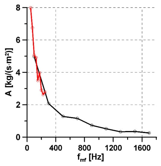
Figure 1.
Amplitude vs. frequency for shock oscillations induced by controlled disturbances introduced upstream of an impinging shock interaction (paper [25], ITAM data).
The studies discussed earlier have primarily focused on the investigation of shock wave interaction with turbulent boundary layers. However, it is important to note that, at sufficiently low Reynolds numbers, the boundary layer can be laminar. In recent years, there has been a growing interest in the interaction of shock waves with laminar boundary layers [26,27]. This increased attention is driven by the potential applications of such flows in the design of partially laminar aircraft and on the blades of turbofan engine compressors intended for high-altitude operation.
If we exclude the cases of very low Reynolds numbers, when interacting with shock waves, a laminar boundary layer typically undergoes a transition to a turbulent state. Sandham [13] provides a classification of such transitional flows. Three scenarios can be distinguished. In the first case, individual turbulent spots impinge on the interaction zone. The dynamics of turbulent spot development during the passage through the interaction zone have been studied, for example, through numerical simulations [28,29]. In the second case, transition occurs in the shear layer above the separation bubble due to instability. Depending on the parameters of the incoming boundary layer, various unstable modes may be present in the flow, experiencing significant amplification in the interaction zone [30]. If laminar flow is maintained up to the shock impingement point, the transition occurs in the attachment region of the flow.
In addition to the two classical cases, namely, shock wave impingement on a boundary layer and flow over a compression ramp [31], an important test case for studying 2D SWBLI is the transonic buffet of an airfoil. Due to its significant practical relevance, this phenomenon has been extensively investigated in experiments [32] and has been shown to correspond to the nonlinear saturation of a global unstable mode by Crouch et al. [33] and Sartor et al. [34]. The presence of feedback and upstream-propagating disturbances undoubtedly adds additional complexity to the case. However, at the same time, these mechanisms allow for a more explicit identification of the oscillation frequencies associated with SWBLI. Recently, buffet studies have also been extended to laminar and transitional regimes [35].
A thorough experimental study was conducted to examine the influence of laminar flow on shock wave dynamics and the presence of the laminar buffet phenomenon on the OALT25 airfoil [36]. The results demonstrate the presence of a distinct critical phenomenon specific to the laminar case, occurring at a frequency around St = 1.1. This is in contrast to the turbulent buffet phenomenon, which occurs at a frequency near St = 0.07. Additionally, a comparable low-frequency dynamics is observed in the laminar case, but at a slightly lower frequency of St = 0.05. These low- and high-frequency modes exhibit similarities to those identified by Finke [37]. Notably, the variations in mode frequency with Mach number and angle of attack align with Finke’s findings.
Despite numerous computational studies that have significantly advanced our understanding of the nature of unsteadiness in SWBLI [5,13], numerical simulations still face challenges in accurately capturing such flow phenomena. These challenges primarily stem from the high computational costs associated with simulating flows at large Reynolds numbers over extended periods of time to accumulate sufficient statistics for analyzing low-frequency flow pulsations [13]. Consequently, experimental investigations of this phenomenon remain highly relevant, especially considering the availability of modern measurement techniques such as hot-wire anemometry and PIV [38,39,40] that provide extensive data on both time-averaged and unsteady flow characteristics.
The utilization of these measurement techniques, together with the introduction of controlled perturbations into the flow and the application of data processing algorithms such as POD and cross-correlation analysis, can provide a comprehensive understanding of the unsteady processes occurring in the SWBLI zone and their interconnections. In this case, a sufficiently powerful short-duration energy source is required for perturbation generation, and an electric discharge has proven to be a suitable option [41]. Similar technology has been widely employed in the study of stability and receptivity of supersonic laminar boundary layers [42,43], where “synthetic jets” generated by electric discharges in a chamber were first utilized.
When a sufficient amount of power is introduced into the flow, such an action can be classified as “flow control”. There are numerous studies available in which electric discharges have been used for controlling SWBLI [5,44]. For instance, Narayanaswamy et al. [45] employed a pulsed plasma jet array actuator to control the separation shock wave of SWBLI on a compression ramp. They demonstrated that the length of the separation bubble decreased when the forcing was applied. Wang et al. proposed a control technique based on the high frequency Counter-flow Plasma Synthetic Jet Actuator (CPSJA) to control a step-induced supersonic separation. The reduction in separation can be attributed to the added momentum in the flow, which disrupts and energizes the boundary layer and the separation region. Additionally, the instability of the separated bubble plays a role, and actuation at a frequency close to the natural frequency of the separation bubble can effectively suppress the separation [46].
Surface arc plasma actuation has been found to be effective in reducing the size of the separation area caused by impinging shock waves. The primary mechanism of control in this case is the generation of oblique shock waves and compressive waves through heating. However, it should be noted that, while the separation phenomenon is delayed, the actual size of the separation area may be enlarged with the implementation of plasma actuation [47].
Kinefuchi et al. [48] have identified two distinct effects of plasma actuators on the shock wave/boundary-layer interaction flow field: heat generation in the boundary layer and vorticity generation near the surface. When the heat generation effect dominates, the interaction between the shock wave and boundary layer intensifies, resulting in an increase in the separation size. However, when vorticity generation prevails, the separation is suppressed due to the transfer of momentum from the main flow to the boundary layer. Electric discharges have also been successfully employed for buffet control on an airfoil [49].
The literature review reveals a notable disparity in the investigation of unsteady processes occurring during the interaction of a shock wave with a boundary layer between laminar and turbulent flows. While there has been extensive research on turbulent flows, there is a lack of available data concerning low-frequency oscillations in the interaction region for the laminar case. This scarcity of data is primarily attributed to the challenges associated with the interpretation of experimental results.
Furthermore, the literature review indicates that there are two sources contributing to the emergence of low-frequency oscillations in the SWBLI region as a result of turbulent interaction. These oscillations are associated with incoming pulsations from the turbulent boundary layer and the inherent global instability of the interaction region. However, the dominance of one mechanism over the other is evidently contingent upon specific conditions. Investigating the laminar SWBLI scenario can shed light on this issue. Given the absence of significant perturbations in the incoming boundary layer for the laminar case, it is anticipated that the mechanism associated with global instability will prevail. In the event that the research reveals significant susceptibility of the interaction region to frequencies closely aligned with those of global instability (St ≈ 0.1–1), this would indirectly confirm the existence of this mechanism in the turbulent scenario.
To address this issue, one approach is to employ the method of artificial disturbances. In this particular study, it was decided to utilize an electric discharge to excite low-frequency disturbances in the laminar boundary layer. By analyzing the development of these disturbances within the shock wave–boundary layer interaction (SWBLI) region, it will be possible to identify and compare the differences in the evolution of unsteady processes between the laminar and turbulent cases.
2. Arrangement of Experiments
The experiments were conducted in the T-325 wind tunnel situated at the Institute of Theoretical and Applied Mechanics (ITAM). The T-325 is an ejector type wind tunnel with exhaust into the atmosphere, and dimensions of the test section are 0.2 × 0.2 × 0.6 m. Some description of the T-325 wind tunnel can be found in the paper [50]. The experiments were conducted under the following free stream flow conditions: Mach number of 1.43, unit Reynolds numbers (Re1) of 10.6 × 10⁶ (1/m) ± 0.2%, stagnation pressure of 70 kPa ± 0.4%, and stagnation temperature (T0) of 296.7 K ± 0.2%. The experimental setup is shown in Figure 2. The study was performed on a flat plate model with a sharp leading edge. The model was set at zero angles of attack. Above the plate a wedge-shaped body, referred to as the shock wave generator, was positioned at an angle of attack of 4°. The coordinate system used in the study is fixed to the model’s leading edge, with the X-axis aligned with the flow direction and the Y-axis pointing upwards perpendicular to the model’s surface.
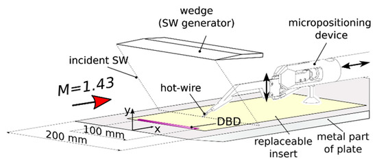
Figure 2.
Experiment scheme.
The model has a span of 200 mm, occupying the entire width of the test section. Structurally the model is composed of multiple parts. The main body is made of steel, while the replaceable insert in the middle section of the model is fabricated from a dielectric material (POM). The width of the replaceable insert is 146 mm. The purpose of this insert is to enable the generation of a dielectric barrier discharge (DBD), which serves as a controlled disturbance source. The DBD is widely used to study the stability of the boundary layer [51,52] and to control the flow [53,54]. The DBD was chosen as the perturbation source, since it allows energy to be supplied uniformly (for low perturbation frequencies) along a wide electrode. This will make it possible to introduce two-dimensional perturbations. The extent of the discharge along the span was 100 mm, allowing the problem to be treated as quasi-two-dimensional.
In this study, measurements of mass flow rate and mass flow rate fluctuations were performed using a constant temperature anemometer (CTA) with a single-wire sensor. The tungsten wire of the sensor had a thickness of 10 μm and a length of 2 mm. The measurements were conducted with an overheat ratio (aw) of 1.75. The bandwidth of the CTA was set to 200 kHz. The ADC PicoScope5443D with a resolution of 14 bits was used to digitize the CTA signal. The data acquisition frequency was 1 MHz, with a recording time of 1 s. The sensor was positioned on a positioning device capable of vertical movements. In turn, the positioning device was securely attached to a rod of the standard coordinate mechanism of the T325 facility, located downstream from the test section. This arrangement allowed measurements to be taken at eight different locations along the X-axis. All measurements were conducted in the model’s plane of symmetry. To obtain quantitative information about the mass flow rate, the methodology described in the paper [55] was applied in this study. In reference [55], flow parameters were measured utilizing two techniques, PIV and CTA. A notable concurrence of approximately 0.5% was achieved between the measurements obtained from these methods. To obtain quantitative information about the mass flow rate, the methodology described in the referenced paper was applied in this study, which assumes the availability of a direct calibration of the CTA (constant temperature anemometer). Additionally, it utilizes additional data on the distribution of the Mach number to account for the changes in the calibration relationship across the shock wave and in the subsonic region near the wall.
The precision of acquiring quantitative data regarding the average mass flow rate through the utilization of CTA is affected by the steadiness of flow parameters during measurements and the precision of calibration. The root-mean-square (RMS) error associated with the calibration process amounted to 1.6%.
Figure 3 depicts the velocity field obtained by the PIV method in the referenced work [55]. It should be noted that the scale differs along the X and Y axes. In this field the main elements of the investigated flow are marked by thick dashed lines: the impinging shock wave, crossing the plate surface at coordinate 132 mm, and the laminar separation located at coordinates 102–135 mm. Other flow features characteristic of this type of shock wave/boundary layer interaction (SWBLI) can also be observed, such as compression waves resulting from the displacement of the flow by the separated region, the reflected shock wave, expansion waves at the end of the separation bubble, and the shock wave at the flow attachment point.
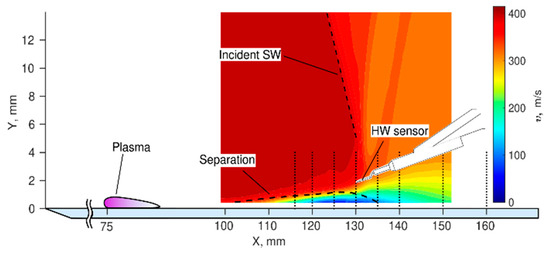
Figure 3.
Velocity field and locations of hot-wire anemometry measurements.
Additionally in this figure, a schematic representation of the plate model, the CTA sensor, and the plasma region located 75 mm from the leading edge of the model and spanning 13 mm are depicted. Vertical dotted lines in X = 116, 120, 125, 130, 135, 140, 150, 160 mm in the figure, show the sections in which hot-wire measurements were carried out by scanning along the Y axis. It is evident that the measurements in the range of X = 116–130 mm were performed in the laminar separation region. At the coordinate X = 135 mm, the impinging shock wave intersects with the boundary layer, leading to the formation of a strong adverse pressure gradient. This leads to the laminar-to-turbulent transition, characterized by an increase in the velocity profile filling of the boundary layer and a sharp growth in its thickness. The turbulent wake behind the SWBLI zone is located in the range of X = 135–160 mm.
The DBD used in these experiments has the following construction: the metallic part of the model served as the open electrode, connected to the grounded part of the discharge power circuit (Figure 4a). The X-coordinate of 75 mm corresponds to the beginning of the dielectric insert. This position of the insert and, consequently, the DBD, was chosen based on the design features of the model to maximize the distance between the disturbance source and the SWBLI zone. To accommodate the second electrode in this insert, a slot with a width of 100 mm along the span was made, where the closed electrode was placed. This electrode was coated with epoxy resin to prevent plasma discharge on the opposite side of the model. The length of the electrode along the X-axis was 10 mm, and the distance between the electrodes in the X-direction was 3 mm. The thickness of the dielectric between the lower electrode and the flow was 2 mm. In the photo in Figure 4b, the plasma region on the model surface and the CTA sensor are visible. It can be observed that the discharge is more stratified in the region between the electrodes, while the glow above the lower enclosed electrode is more homogeneous.
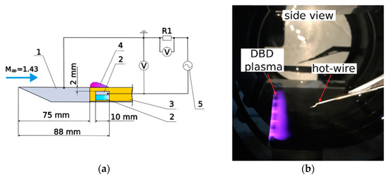
Figure 4.
(a) Design of the DBD and electrical circuit of the experiment and (b) photo of DBD during experiment (1—steel part of model, 2—HV electrode, 3—POM part of model, 4—plasma region, 5—HV source).
During the experiments, a sinusoidal voltage with the parameters specified in Table 1 was applied to the electrodes. The voltage was tuned in such a way that the plasma region would occur at the edge of the open electrode and extend downstream to the trailing edge of the lower enclosed electrode. The carrier frequency (fcarry) of 17.6 kHz is the resonant frequency for the oscillatory circuit formed by the power supply of the DBD. The main characteristics of this circuit are determined by the discharge capacitance and the inductance of the transformer coil of the AC power source. This frequency is an order of magnitude higher than the frequencies typical for the SWBLI zone, and the energy supply at such a frequency can be considered quasi-stationary. To generate low-frequency disturbances, the quasi-stationary energy supply at the carrier frequency (fcarry) was modulated at the modulation frequency (fmod) with a duty cycle of 0.5. The values of the frequencies used in the experiment are provided in Table 1. This frequency range is equal to Strouhal numbers based on the length of the separation bubble, from 0.04 to 0.13. The current and voltage on the electrodes were measured using a digital oscilloscope RIGOL DS1102E. The length of the measurement cycle was 5.4 ms, and the recording was averaged over eight cycles. The voltage was measured using a high-voltage probe, Tektronix P6015A. The current was measured by the voltage drop on the resistor R1 = 107 Ohms.

Table 1.
Sinusoidal voltage with the parameters applied to the electrodes.
Figure 5 shows examples of current and voltage oscillograms on the DBD for the case of fmod = 500 Hz during one modulation period, T = 1/fmod, as shown in Figure 5a, and during one carrier signal period, T = 1/fcarry, as shown in Figure 5b. From Figure 5a it can be observed that the system exhibits inertia and requires several periods of oscillations at the carrier frequency for the voltage and current amplitudes to reach the desired value. Inertia is also observed during the decay. The oscillogram in Figure 5b was obtained by averaging the oscillogram in Figure 5a over a time interval from 0.28 ms to 0.8 ms, covering a whole number of oscillations at the carrier frequency.
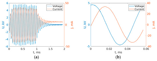
Figure 5.
Voltages and current oscillogram for fmod = 500 Hz during one period (a) 1/fmod and for (b) 1/fcarry.
Figure 6 presents the values of electrical power consumed by the DBD and the voltage amplitudes on the electrodes as a function of the modulation frequency. The average values shown by the symbols, as well as the magnitude of the confidence intervals, were calculated for each fmod based on eight measurements taken at different positions along the X-axis. As can be seen from this figure, there is a variation in voltage amplitude of approximately ±8% and in power of approximately ±17% during the experiments. However, further data analysis revealed that this variation does not have a significant impact on the development of disturbances and is likely to have a weak effect on their initial amplitude.
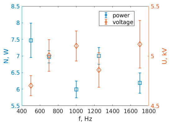
Figure 6.
Electrical power and voltage amplitude.
3. Numerical Setup
The primary objective of the numerical study was to conduct a qualitative analysis of the impact mechanism of a dielectric barrier discharge on the SWBLI. The rationale behind adopting a numerical approach is attributed to the intricate nature of the generation of low-frequency disturbances in experiments. Given that modulation of a high-frequency signal is employed for this purpose, a question arises regarding the nature of the introduced perturbations. It was imperative to ascertain whether this approach indeed facilitates the exploration of low-frequency disturbances, or if it predominantly examines higher-frequency disturbances introduced by the discharge.
To address this inquiry, it suffices to examine the evolution of disturbances in the laminar region since disturbances in the turbulent flow region originate in the laminar boundary layer. Consequently, to tackle this issue, it is adequate to model the laminar boundary layer and the separation bubble in a two-dimensional configuration (as the discharge mainly introduces two-dimensional perturbations). Direct numerical simulation of the flow in the turbulent region is not required in this case.
However, given that the flow consists of both laminar and turbulent regions, a methodology is needed that accommodates both zones to ensure accurate modeling of the laminar separation bubble. For this purpose, it was decided to employ URANS simulation, with a fixed transition point. The mesh quality within the laminar region and the time step must enable the resolution of disturbances across the entire frequency spectrum under investigation.
It is evident that, for a quantitative numerical analysis of such a problem, more precise modeling methods such as DNS would be necessary. However, for the objectives of this study, utilizing URANS with spatial and temporal resolutions adequate for the simulation of disturbances in the laminar region is well-justified.
Numerical simulations were conducted using the ANSYS Fluent software package. The 2D unsteady Navier−Stokes equations were solved using a density-based solver. An explicit second-order scheme in space and an explicit first-order scheme in time were applied, together with the AUSM method for splitting the convective fluxes. RANS simulations were conducted using the κ-ω SST turbulent model. A structured block grid refined in the wedge region and in the wake behind the wedge was used (Figure 7). Grid refinement in the boundary layer ensured y+ ≈ 0.2–1 in the entire computational domain. The total number of cells was approximately 1.2 million. The physical size of the computational domain was 255 × 92 mm. The experimental freestream parameters were specified at the inlet boundary of the computational domain (P0 = 70 kPa, T0 = 298 K, M = 1.43). The boundary of the plate and wedge model was subjected to adiabatic boundary conditions. The symmetry condition was selected at the upper boundary and upstream of plate. In the calculation, the effects of a real gas were not taken into account since the heating of the flow did not exceed a few degrees Celsius. Viscosity was calculated using the Sutherland equation. The origin of coordinates coincided with the leading edge of the plate.
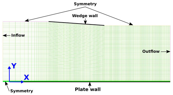
Figure 7.
Computational grid (only every 10 cells are displayed).
The number of cells in the boundary layer was approximately 80–130. The mesh was refined towards the model wall and the value of x+ was approximately equal to 10–20 in the SWBLI zone. Mesh convergence was studied by using the wall viscous drag as criteria. The difference in drag between the main mesh (1.2 million cells) and a more accurate/coarser mesh (3/0.4 million cells) did not exceed 0.5%. The choice of a 1.2 million grid was motivated by the desire to resolve potential high-frequency disturbances that could develop on the fronts of the introduced perturbations. In the study [56], it was established that, in order to resolve disturbances in the ANSYS Fluent, a minimum of 80 cells per wavelength is required, allowing for the simulation of two-dimensional disturbances with frequencies of at least 50–100 kHz. The study [57] demonstrated a good agreement between the DNS and RANS calculations using the κ-ω SST turbulence model with a fixed transition point for this specific computational case. Furthermore, this study demonstrates a favorable agreement between RANS data and experimental results in the region of the laminar separation bubble. Therefore, the calculations were performed using this turbulence model. The laminar–turbulent transition point was set as a fixed value. Up to X = 131 mm, the flow was assumed to be laminar. To enforce this condition the turbulent kinetic energy was set to zero before X = 131 mm.
The excitation of disturbances by the DBD was simulated by volumetric energy deposition in the near-wall region. The feasibility of simulating plasma through volumetric energy deposition has been demonstrated in studies [58,59]. In these works, the power of the plasma source and experimental parameters closely align with those of the current study, which provides a high likelihood of asserting the applicability of this approach for simulating disturbance introduction mechanisms. The energy was uniformly deposited in the region of X = 75–88 mm and Y = 0–0.4 mm. The average power of the discharge was approximately 7 W (70 W/m). To clarify the mechanism of excitation of the disturbances in the experiment, three series of calculations were performed, in which the temporal energy deposition was modeled in three different ways.
In the first case, a square function with a duty cycle of 0.5 (Figure 8) was used to model the energy deposition. The second case employed a sinusoidal law for the temporal variation of energy deposition. Frequencies corresponding to fmod = 500, 750, 1250, and 1700 Hz were considered for the first and second methods. In the third case, energy was deposited according to a sinusoidal law at the carrier frequency of 17 kHz, which was modulated by a square function with a duty cycle of 0.5 at frequencies fmod.
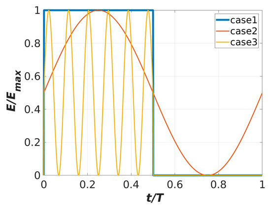
Figure 8.
Dependence of the volume energy release on time.
4. Experimental Results
Figure 9a,b illustrates an example of CTA data obtained in the laminar separation bubble region for the case without discharge. The velocity profile can be divided into two regions. The first region, Y = 0–0.5 mm for X = 116 mm and Y = 0–1 mm for X = 125 mm, corresponds to the separation bubble. The second region, Y = 0.5–1.2 mm for X = 116 mm and Y = 1–2 mm for X = 125 mm, corresponds to the shear layer above the laminar bubble. It is important to note that, in the analysis of the data, the use of a single-wire probe should be taken into account, as it does not detect the reverse flow. Furthermore it is worth noting that the introduction of the disturbances by DBD did not lead to significant changes in the mean flow.
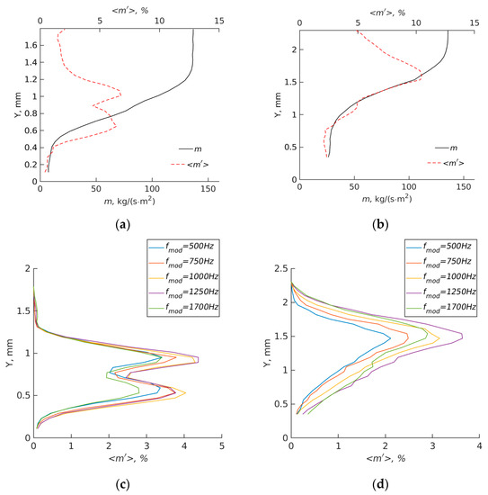
Figure 9.
Top–distribution of the mean value and RMS of mass flow rate for case without discharge, bottom–distribution of RMS mass flow disturbances generated by the discharge of various frequencies ((a,c)—X = 116 mm; (b,d)—X = 125 mm).
In the distribution of RMS values of fluctuations shown in Figure 9, two main peaks can be observed. The first peak is located in the region of the shear layer above the laminar bubble (Y ≈ 1.1 mm for X = 116 mm and Y ≈ 1.6 mm for X = 125 mm), while the second peak is situated at the boundary between the separated flow region and the boundary layer (Y ≈ 0.6 mm for X = 116 mm and Y ≈ 1.1 mm for X = 125 mm).
To extract the fluctuations associated with the DBD effect from the CTA signal, window averaging was performed. The size of the window was chosen to be equal to the voltage modulation period (Tmod = 1/fmod). To obtain phase information CTA measurements were synchronized with the measurements of the electrical parameters of the discharge. From the data presented in Figure 9c,d, it can be observed that the DBD excites the disturbances in the boundary layer. Moreover, the amplitude of these disturbances is dependent on the discharge frequency (fmod). It is evident that, at the beginning of the separation region (Figure 9c), the magnitudes of the RMS fluctuations induced by the discharge exhibit similar distributions and comparable amplitudes along the height. The positions of the fluctuation peaks coincide with the data obtained without the discharge (Figure 9a); in the case with the discharge, the amplitudes of the fluctuations are approximately equal in both peaks.
The obtained data indicates that the method used in the study for introducing disturbances allowed for the introduction of fluctuations with approximately equal amplitudes within the investigated frequency range. Furthermore, the profile of these fluctuations qualitatively resembles that of natural fluctuations. The data obtained at X = 120 mm are qualitatively and quantitatively similar to the data at X = 116 mm and are therefore not shown separately. Downstream at X = 125 mm, there is still a qualitative agreement in the distribution of the discharge-induced fluctuations. However when comparing the amplitudes, it can be observed that the maximum fluctuations occur in the case of 1250 Hz, which are twice as large as those in the low-frequency case. The position of the maximum fluctuation approximately coincides with the position of the maximum fluctuations in the case without discharge, which is located in the shear layer.
At a downstream location in the end of the separation region at X = 130 mm, the distribution of mean and RMS mass flow rate values (Figure 10a) qualitatively resembles the data obtained at X = 125 mm. However the DBD (Figure 10c) leads to a different distribution of RMS compared to the data obtained at X = 125 mm. For the X = 130 mm profile, at high frequencies fmod = 1000–1700 Hz, two peaks of fluctuations can be observed, while no clear peak of fluctuations is observed for low frequencies fmod = 500–750 Hz. From the figure, it is evident that the amplitude of the discharge-induced disturbances increases significantly with increasing fmod. The maximum fluctuations are observed at frequencies of 1250 and 1700 Hz.
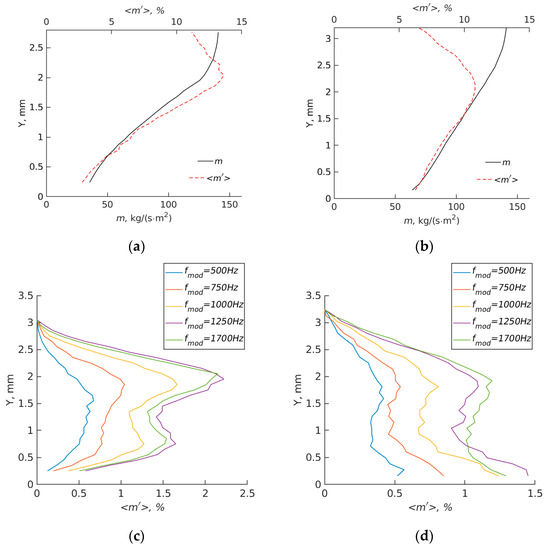
Figure 10.
Top–distribution of the mean value and RMS of mass flow rate for case without discharge, bottom–distribution RMS mass flow disturbances generated by the discharge at different frequencies ((a,c)—X = 130 mm; (b,d)—X = 135 mm).
The section X = 135 mm is located in the transition region, as indicated by the increase in the fullness of the mass flow profile (Figure 10b). The transition to turbulent flow leads to significant changes in the distribution of RMS fluctuations induced by the discharge (Figure 10d). The main peak of disturbances is observed near the wall, in contrast to the data obtained in the laminar region (Figure 9c,d and Figure 10c), where the fluctuations near the wall tended to approach zero. As the distance from the wall increases, the disturbances gradually decay. Similar to the section X = 130 mm, the maximum disturbances were obtained for frequencies fmod = 1250–1700 Hz. Decreasing the frequency of induced disturbances leads to a reduction in the magnitude of the RMS fluctuations of the disturbances.
In Figure 11a,b, the data obtained in the turbulent wake region are shown. It is evident that as the streamwise coordinate increases the fullness of the mass flow profile increases, which can be interpreted as the gradual approach of the near-wall flow to an equilibrium turbulent boundary layer. Let us consider what happens with the fluctuations induced by the DBD discharge in the wake region. At X = 140 mm, the dependence of the fluctuation amplitude on frequency (Figure 11c) qualitatively resembles the profiles observed at X = 125–135 mm. The maximum level of fluctuations is achieved near the wall, similar to the X = 135 mm profile, but the fluctuation magnitudes decrease as we move downstream.
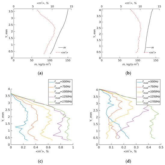
Figure 11.
Top–distribution of the mean value and RMS of mass flow rate for case without discharge, bottom–distribution RMS mass flow disturbances generated by the discharge at different frequencies ((a,c)—X = 140 mm; (b,d)—X = 150 mm).
As we move further downstream to X = 150 mm (Figure 11d), significant differences in the distribution of the RMS fluctuations induced by the discharge can be observed depending on fmod. For the low frequency fmod = 500 Hz, the maximum fluctuations are located near the wall and, as the distance from the wall increases, there is a monotonic decrease of their amplitude. For frequencies fmod = 750–1250 Hz, the maximum RMS values are observed in the region Y ≈ 3 mm, and the disturbance magnitude decreases close to the wall. For the maximum frequency fmod = 1700 Hz, the RMS fluctuations of mass flow rate are approximately constant in the whole boundary layer region. From Figure 9, Figure 10 and Figure 11, it is evident that there is a predominantly decreasing trend in the amplitudes of disturbances introduced by the discharge as we move downstream. In the X = 160 mm section, the disturbances induced by the discharge approach zero and are therefore not discussed.
Figure 12 depicts the periodic variation of mass flow rate over time induced by the disturbance introduced by the discharge at a frequency of fmod = 500 Hz. From the figure, it can be observed that in the beginning part of the interaction region (X = 116–125 mm) the oscillations in the shear layer and the separation bubble occur nearly in phase. However, in the laminar–turbulent transition region and the wake region (X = 135–150 mm), the near-wall disturbances are phase-shifted relative to the disturbances closer to the boundary layer edge. The low-frequency disturbances introduced by the discharge lead to fluctuations in the size of the separation region, resulting in phased pulsations in the separation region. Furthermore the oscillation of the separation zone can lead to more complex flow changes in the wake characterized by deceleration near the wall when acceleration occurs in the outer part of the boundary layer.
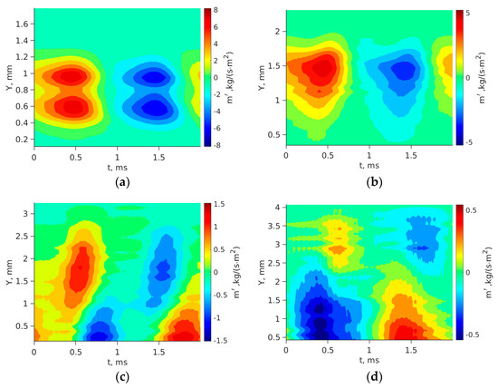
Figure 12.
Oscillogram of the disturbances of mass flow generated by a discharge along the boundary layer at frequency fmod = 500 Hz–((a)—X = 116 mm, (b)—X = 125 mm, (c)—X = 135 mm, (d)—X = 150 mm).
Figure 13 shows the effect of disturbance frequency on the oscillogram of mass flow rate in the separation region (X = 130 mm). It is evident that the main difference lies in the increase of the relative slope of disturbances with increasing disturbance frequency. However, the temporal shift between the maximum mass flow rate near the boundary layer edge (Y ≈ 2.3 mm) and near the wall (Y ≈ 0.5 mm) is independent of the frequency and remains around 300 μs.
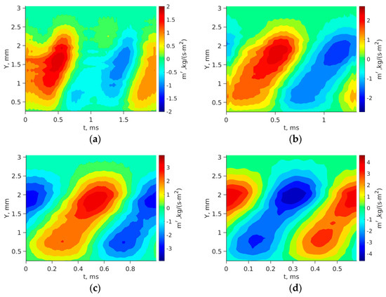
Figure 13.
Oscillogram of the disturbances of mass flow generated by a discharge along the boundary layer at X = 130 mm ((a)—fmod = 500 Hz, (b)—fmod = 750 Hz, (c)—fmod = 1000 Hz, (d)—fmod = 1700 Hz).
Figure 14 presents data similar to Figure 13 but obtained in the wake region (X = 150 mm). In contrast to the data obtained in the downstream part of the separation region (X = 130 mm), changing the frequency leads to significant restructuring of the oscillogram of mass flow rate in the boundary layer. For instance, at the maximum frequency of fmod = 1700 Hz, the change in mass flow rate occurs with a single phase along the entire boundary layer, whereas at the frequency of fmod = 750 Hz disturbances near the wall are out of phase with disturbances near the boundary layer edge. One possible explanation for this phenomenon is the presence of two distinct disturbances in the wake (near the wall and near the boundary layer edge) propagating with different phase speeds.
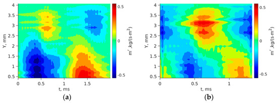
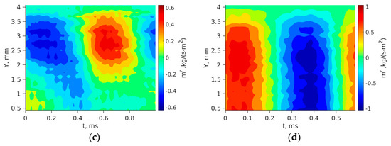
Figure 14.
Oscillogram of the disturbances of mass flow generated by a discharge along the boundary layer at X = 150 mm ((a)—fmod = 500 Hz, (b)—fmod = 750 Hz, (c)—fmod = 1000 Hz, (d)—fmod = 1700 Hz).
The summarized results of the experiments are presented in Figure 15. In Figure 15a, the vertical position of the RMS maximum along the plate for different frequencies fmod can be observed. Since some profiles of the RMS pulsations of mass flow exhibited two maxima, it was decided to analyze only the peak closer to the boundary layer edge. This approach assumes that it allows for the examination of the development of a single type of disturbance. It is evident that the position of the peak weakly depends on the frequency and for the most part moves away from the wall with increasing longitudinal coordinate due to growth of the boundary layer thickness, except for the section at X = 160 mm, where the disturbance amplitudes approach zero.
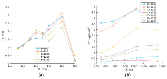
Figure 15.
(a)—Location in the boundary layer of the maximum amplitude of disturbances introduced by the discharge along the plate, (b)—maximum amplitude of disturbances vs. frequency at different longitudinal coordinates.
Let us consider the variation in the amplitudes of disturbances introduced by the discharge (Figure 15b). As noted earlier in the separated flow region (X = 120–125 mm), the maximum pulsation is observed at a frequency of 1250 Hz. Further downstream in the region near the incident shock wave (X = 130 mm), low-frequency disturbances rapidly decay and there is also a leveling off of the amplitudes of disturbances developing at frequencies between 1250 and 1700 Hz. In the turbulent wake region (X = 135–150 mm), similar trends of increasing disturbance amplitudes with frequency are observed. Moreover, the relative amplitudes of disturbances at different frequencies are approximately preserved. As the longitudinal coordinate increases, there is a gradual attenuation of the disturbances introduced by the discharge. In the final region at X =160 mm, the maximum pulsation is observed only near the wall, making it inappropriate to compare these data with the results obtained in upstream sections. It should be noted that the relationship between disturbance amplitude and frequency does not correlate with the graphical representation of electrical power, as depicted in Figure 6.
The experimental results demonstrate that the largest disturbances develop at frequencies ranging from 1250 to 1700 Hz corresponding to St ≈ 0.1–0.13. As the frequency of the introduced disturbances decreases, their amplitude decreases as they propagate into the SWBLI region.
From the obtained data, it is evident that the primary development of disturbances within the laminar separation bubble region occurs within the shear layer, precisely in the zone of maximal mass flow rate gradients. Moreover, a notable agreement exists between the amplitude distributions of inherent disturbances and those of the introduced disturbances within the shear layer. This suggests the possibility that the introduced disturbances evolve as a wave-like process. In the investigated low-frequency range, these disturbances exhibit a damping behavior. Notably, the presence of a distinctive frequency range around St ≈ 0.1–0.13 could signify the influence of global instability within the laminar region, a matter which will be addressed later.
The introduced low-frequency disturbances have a limited impact on the actual mechanism of laminar-to-turbulent transition, primarily due to their much larger scale compared to the characteristic scales of the boundary and shear layers. Therefore, it is apparent that both in the case of inherent disturbances and the introduction of artificial disturbances, the transition occurs following a similar scenario where higher-frequency disturbances play a decisive role. Despite this, when altering the frequency of the introduced low-frequency disturbances, the turbulence characteristics in the wake change significantly. This leads to the presumption that these introduced disturbances influence, at the very least, the oscillations of the transition point within the attachment region of the flow.
Regrettably, within the scope of this experimental setup, this specific flow region was not extensively investigated. To address this, further research, preferably numerical, is required. In this context, the data obtained in this study could serve as a verification benchmark for computational simulations. The obtained results for the laminar case significantly differ from the data obtained under similar conditions in the case of turbulent incoming boundary layer. When the shock wave interacts with the turbulent boundary layer, a monotonic decrease in disturbance amplitude with increasing frequency was observed [25], as shown in Figure 1. It can be hypothesized that the selectivity in frequency is due to the presence of a global instability in the laminar separation flow which is influenced by the disturbances generated by the discharge. However, these disturbances rapidly decay in the turbulent wake region.
5. Numerical Results
Figure 16 presents the results of numerical simulation conducted for the test case with the introduction of a sinusoidal disturbance (case 2) at a frequency of 1250 Hz. The color map represents the RMS value of the streamwise velocity pulsations, while the contour lines correspond to the mean velocity magnitude. The vertical black lines represent the positions of velocity profiles measured in the experiment. The calculation results show good agreement of the mean flow in the laminar separation zone compared to the experimental data. In the turbulent wake region, a significantly thinner boundary layer is observed in the simulation. Therefore, further analysis will focus only on the data obtained in the laminar flow region. It is evident that the main disturbances develop within the shear layer of the laminar bubble.
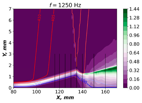
Figure 16.
RMS distribution of velocity fluctuations.
Figure 17 presents numerical results obtained when introducing disturbances in the form of a square pulse (case 1, Figure 8). It is evident (Figure 17a,b) that for this case the disturbance in the boundary layer takes the form of a wave packet with pronounced low-frequency and high-frequency waves. The characteristic frequency of the high-frequency disturbances arising on the leading and trailing edges of the main pulse significantly exceeds the frequency fmod. As the flow progresses downstream, the content of the wave packet undergoes significant transformation. High-frequency disturbances generated on the leading and trailing edges become more prominent while the main disturbance decays. From the distribution of the RMS velocity magnitude (Figure 17c,d), it is clear that the maximum for these disturbances is observed in the region of the maximum velocity gradient within the shear layer. In the reattachment region, the disturbance amplitude remains approximately constant. These findings qualitatively agree with the experimental data.
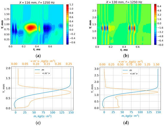
Figure 17.
(a,b) Oscillogram of the disturbances of mass flow, (c,d) distribution of the mean value and RMS of mass flow rate at fmod = 1250 Hz, case 1 ((a,c)—X = 116 mm, (b,d)—X = 130 mm).
From Figure 17c,d, it is evident that there is an increase in disturbance amplitude by more than a factor of 4 from X = 116 mm to X = 130 mm. This result contradicts the experimental data which showed a weak decay of disturbances along the streamwise coordinate. It should be noted that, when introducing disturbances in the form of a sinusoidal signal with a frequency of 17 kHz, modulated by a square pulse with frequency fmod (case 3, Figure 8), the obtained results were quantitatively and qualitatively similar to Figure 17 (case 1, Figure 8). The main difference was that the frequency of the wave packet remained constant.
Figure 18 shows data similar to the results shown in Figure 17 but obtained by introducing disturbances in the form of a sinusoidal signal (case 2, Figure 8). It is evident that, in this case (Figure 18a,b), the predominant disturbance propagates as a sinusoidal wave with a frequency corresponding to the input disturbance frequency fmod. The distribution of RMS values of velocity fluctuations along the boundary layer qualitatively resembles the data obtained in Figure 17. However, the maximum magnitude of the fluctuations decays with increasing longitudinal distance, which is similar to the experimental data.
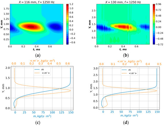
Figure 18.
(a,b) Oscillogram of the disturbances of mass flow, (c,d) distribution of the mean value and RMS of mass flow rate at fmod = 1250 Hz, case 2 ((a,c)—X = 116 mm, (b,d)—X = 130 mm).
The numerical simulation data vividly illustrate that the results obtained from energy input using low-frequency rectangular pulse and rectangular pulse modulation of a high-frequency signal fail to even qualitatively align with the experimental outcomes. The most favorable qualitative agreement was achieved with the results of numerical simulations in case 2, where solely low-frequency sinusoidal disturbances were introduced. In the experiment, significant influence from high-frequency disturbances, which could have been introduced by the discharge and are present in computational cases 1 and 3, was not observed.
The reason for the particularly successful introduction of only low-frequency disturbances using DBD in the experiment might be attributed to the intricate nature of the streamers generated during DBD operation, which could be the main source of the introduced disturbances. Nonetheless, to provide a more precise answer to this question, dedicated studies are necessary. Nevertheless, the most crucial outcome is that the methods employed in the experiment for disturbance introduction and data analysis enable the exploration of the evolution of low-frequency periodic two-dimensional disturbances that closely resemble sinusoidal disturbances. This lays the foundation for the future utilization of this approach to introduce two-dimensional low-frequency sinusoidal disturbances.
6. Conclusions
This paper presents a method for studying the response of the interaction between a shock wave and a laminar boundary layer to two-dimensional disturbances generated by a dielectric barrier discharge.
The experiments were conducted on a flat plate model at a Mach number of M = 1.43. A wedge was used to generate the impinging shock wave above the plate.
The outcomes of qualitative numerical analysis have enabled the establishment that the dielectric barrier discharge can indeed serve as a source for generating low-frequency two-dimensional disturbances. This finding opens up vast opportunities for employing this method in the exploration of various separation regions, particularly in experimental scenarios involving separation flows. This is because the characteristic frequencies associated with these flows predominantly fall within the low-frequency range (<1 kHz).
During the experiments, it was observed that the most prominent disturbances develop at characteristic frequencies around St ≈ 0.1–0.13. These findings significantly deviate from the results obtained for the turbulent SWBLI scenario, where disturbances exhibit a monotonic attenuation as frequency increases. This discrepancy implies the presence of a global instability mechanism within this laminar SWBLI, exerting a more substantial influence in comparison to fully turbulent interactions. Given the nature of this laminar case, where the energy of incoming disturbances is limited, the absence of significant low-frequency disturbances in the separation region indirectly supports the hypothesis of the predominant impact of incoming turbulent pulsations on low-frequency oscillations in the SWBLI region for turbulent cases.
Within the interaction region, disturbances experience a gradual decay as the flow progresses downstream. It was shown that manipulating the frequency of the introduced disturbance has a minimal impact on the distribution of disturbance amplitude along the flow in the laminar bubble region. However, it can substantially alter the distribution of velocity fluctuations in the turbulent wake region. The acquired data leads to the hypothesis that low-frequency disturbances influence the location of the laminar-to-turbulent transition point and consequently affect the flow characteristics in the turbulent wake region.
Author Contributions
Conceptualization, P.P. and A.S.; Methodology, P.P. and O.V.; Formal analysis, P.P. and A.S.; Investigation, O.V.; Data curation, P.P. and O.V.; Writing—original draft, P.P., O.V. and A.S.; Writing—review & editing, A.S. and O.V. All authors have read and agreed to the published version of the manuscript.
Funding
The research was carried out within the state assignment of Ministry of Science and Higher Education of the Russian Federation.
Acknowledgments
The study was conducted at the Equipment Sharing Center «Mechanics» of ITAM SB RAS.
Conflicts of Interest
The authors declare no conflict of interest.
References
- Gaitonde, D.V. Progress in shock wave/boundary layer interactions. Prog. Aerosp. Sci. 2015, 72, 80–99. [Google Scholar] [CrossRef]
- Dolling, D.S. Fifty years of shock-wave/boundary-layer interaction research: What next? AIAA J. 2001, 39, 1517–1531. [Google Scholar] [CrossRef]
- Babinsky, H.; Harvey, J. (Eds.) Shock Wave-Boundary-Layer Interactions; Cambridge Aerospace Series; Cambridge University Press: Cambridge, UK; New York, NY, USA, 2011; ISBN 9780521848527. [Google Scholar]
- Huang, W.; Wu, H.; Yang, Y.-G.; Yan, L.; Li, S.-B. Recent advances in the shock wave/boundary layer interaction and its control in internal and external flows. Acta Astronaut. 2020, 174, 103–122. [Google Scholar] [CrossRef]
- Ligrani, P.M.; McNabb, E.S.; Collopy, H.; Anderson, M.; Marko, S.M. Recent investigations of shock wave effects and interactions. Adv. Aerodyn. 2020, 2, 4. [Google Scholar] [CrossRef]
- Hadjadj, A.; Dussauge, J.P. Shock wave boundary layer interaction. Shock Waves 2009, 19, 449–452. [Google Scholar] [CrossRef]
- Pasquariello, V.; Hickel, S.; Adams, N.A. Unsteady effects of strong shock-wave/boundary-layer interaction at high Reynolds number. J. Fluid Mech. 2017, 823, 617–657. [Google Scholar] [CrossRef]
- Polivanov, P.A.; Sidorenko, A.A.; Maslov, A.A. Correlation study in shock wave–turbulent boundary layer interaction. Shock Waves 2011, 21, 193–203. [Google Scholar] [CrossRef]
- Dussauge, J.P.; Piponniau, S. Shock/boundary-layer interactions: Possible sources of unsteadiness. J. Fluids Struct. 2008, 24, 1166–1175. [Google Scholar] [CrossRef]
- Grilli, M.; Schmid, P.J.; Hickel, S.; Adams, N.A. Analysis of unsteady behaviour in shockwave turbulent boundary layer interaction. J. Fluid Mech. 2012, 700, 16–28. [Google Scholar] [CrossRef]
- Dolling, D.S.; Murphy, M.T. Unsteadiness of the separation shock wave structure in a supersonic compression ramp flowfield. AIAA J. 1983, 21, 1628–1634. [Google Scholar] [CrossRef]
- Clemens, N.T.; Narayanaswamy, V. Low-frequency unsteadiness of shock wave/turbulent boundary layer interactions. Annu. Rev. Fluid Mech. 2014, 46, 469–492. [Google Scholar] [CrossRef]
- Vanstone, L.; Clemens, N.T. Proper orthogonal decomposition analysis of swept-ramp shock-wave/boundary-layer unsteadiness at Mach 2. AIAA J. 2019, 57, 3395–3409. [Google Scholar] [CrossRef]
- Sandham, N.D. Shock-wave/boundary-layer interactions. NATO Res. Technol. Organ. (RTO)–Educ. Notes Paper 2011, 5, 1–18. [Google Scholar]
- Ganapathisubramani, B.; Clemens, N.T.; Dolling, D.S. Effects of upstream boundary layer on the unsteadiness of shock-induced separation. J. Fluid Mech. 2007, 585, 369–394. [Google Scholar] [CrossRef]
- Ganapathisubramani, B.; Clemens, N.T.; Dolling, D.S. Low-frequency dynamics of shock-induced separation in a compression ramp interaction. J. Fluid Mech. 2009, 636, 397–425. [Google Scholar] [CrossRef]
- Humble, R.A.; Elsinga, G.E.; Scarano, F.; Van Oudheusden, B.W. Three-dimensional instantaneous structure of a shock wave/turbulent boundary layer interaction. J. Fluid Mech. 2009, 622, 33–62. [Google Scholar] [CrossRef]
- Robinet, J.C. Bifurcations in shock-wave/laminar-boundary-layer interaction: Global instability approach. J. Fluid Mech. 2007, 579, 85–112. [Google Scholar] [CrossRef]
- Touber, E.; Sandham, N.D. Large-eddy simulation of low-frequency unsteadiness in a turbulent shock-induced separation bubble. Theor. Comput. Fluid Dyn. 2009, 23, 79–107. [Google Scholar] [CrossRef]
- Piponniau, S.; Dussauge, J.P.; Debieve, J.F.; Dupont, P. A simple model for low-frequency unsteadiness in shock-induced separation. J. Fluid Mech. 2009, 629, 87–108. [Google Scholar] [CrossRef]
- Wu, M.; Martin, M.P. Analysis of shock motion in shockwave and turbulent boundary layer interaction using direct numerical simulation data. J. Fluid Mech. 2008, 594, 71–83. [Google Scholar] [CrossRef]
- Plotkin, K.J. Shock wave oscillation driven by turbulent boundary-layer fluctuations. AIAA J. 1975, 13, 1036–1040. [Google Scholar] [CrossRef]
- Poggie, J.; Smits, A.J. Experimental evidence for Plotkin model of shock unsteadiness in separated flow. Phys. Fluids 2005, 17, 018107. [Google Scholar] [CrossRef]
- Touber, E.; Sandham, N.D. Low-order stochastic modelling of low-frequency motions in reflected shock-wave/boundary-layer interactions. J. Fluid Mech. 2011, 671, 417–465. [Google Scholar] [CrossRef]
- Doerffer, P.; Hirsch, C.; Dussauge, J.P.; Babinsky, H.; Barakos, G.N. WP-3 Flow Control Application (Holger Babinsky). In Unsteady Effects of Shock Wave Induced Separation; Notes on Numerical Fluid Mechanics and Multidisciplinary Design; Springer: Berlin/Heidelberg, Germany, 2010; Volume 114. [Google Scholar] [CrossRef]
- Kolesnik, E.; Smirnov, E.; Babich, E. Dual Numerical Solution for 3D Supersonic Laminar Flow Past a Blunt-Fin Junction: Change in Temperature Ratio as a Method of Flow Control. Fluids 2023, 8, 149. [Google Scholar] [CrossRef]
- Polivanov, P.A.; Sidorenko, A.A.; Maslov, A.A. The Influence of the Laminar-Turbulent Transition on the Interaction between the Shock Wave and Boundary Layer at a Low Supersonic Mach Number. Tech. Phys. Lett. 2015, 41, 933–937. [Google Scholar] [CrossRef]
- Krishnan, L.; Sandham, N.D. Strong Interaction of a Turbulent Spot with a Shock-Induced Separation Bubble. Phys. Fluids 2007, 19, 016102. [Google Scholar] [CrossRef]
- Quadros, R.; Bernardini, M. Numerical Investigation of Transitional Shock-Wave/Boundary-Layer Interaction in Supersonic Regime. AIAA J. 2018, 56, 2712–2724. [Google Scholar] [CrossRef]
- Yao, Y.; Krishnan, L.; Sandham, N.D.; Roberts, G.T. The Effect of Mach Number on Unstable Disturbances in Shock/Boundary-Layer Interactions. Phys. Fluids 2007, 19, 054104. [Google Scholar] [CrossRef]
- Babinsky, H.; Dupont, P.; Polivanov, P.; Sidorenko, A.; Bur, R.; Giepman, R.; Schrijer, F.; Van Oudheusden, B.; Sansica, A.; Sandham, N.; et al. WP-2 Basic Investigation of Transition Effect. In Transition Location Effect on Shock Wave Boundary Layer Interaction; Doerffer, P., Flaszynski, P., Dussauge, J.-P., Babinsky, H., Grothe, P., Petersen, A., Billard, F., Eds.; Springer International Publishing: Cham, Switzerland, 2021; Volume 144, pp. 129–225. ISBN 9783030474607. [Google Scholar]
- Jacquin, L.; Molton, P.; Deck, S.; Maury, B.; Soulevant, D. Experimental Study of Shock Oscillation over a Transonic Supercritical Profile. AIAA J. 2009, 47, 1985–1994. [Google Scholar] [CrossRef]
- Crouch, J.D.; Garbaruk, A.; Magidov, D.; Travin, A. Origin of Transonic Buffet on Aerofoils. J. Fluid Mech. 2009, 628, 357–369. [Google Scholar] [CrossRef]
- Sartor, F.; Mettot, C.; Sipp, D. Stability, Receptivity, and Sensitivity Analyses of Buffeting Transonic Flow over a Profile. AIAA J. 2015, 53, 1980–1993. [Google Scholar] [CrossRef]
- Brion, V.; Dandois, J.; Abart, J.-C.; Paillart, P. Experimental Analysis of the Shock Dynamics on a Transonic Laminar Airfoil. In Proceedings of the Progress in Flight Physics; Knight, D., Bondar, Y., Lipatov, I., Reijasse, P., Eds.; EDP Sciences: Krakow, Poland, 2017; pp. 365–386. [Google Scholar]
- Brion, V.; Dandois, J.; Mayer, R.; Reijasse, P.; Lutz, T.; Jacquin, L. Laminar Buffet and Flow Control. Proc. Inst. Mech. Eng. Part G J. Aerosp. Eng. 2020, 234, 124–139. [Google Scholar] [CrossRef]
- Finke, K. Shock Oscillations in Transonic Flows and Their Prevention. In Proceedings of the Symposium Transsonicum II; Oswatitsch, K., Rues, D., Eds.; Springer: Berlin/Heidelberg, Germany, 1976; pp. 57–65. [Google Scholar]
- Dupont, P.; Piponniau, S.; Sidorenko, A.; Debiève, J.F. Investigation by Particle Image Velocimetry Measurements of Oblique Shock Reflection with Separation. AIAA J. 2008, 46, 1365–1370. [Google Scholar] [CrossRef]
- Threadgill, J.A.S.; Little, J.C. Volumetric Study of a Turbulent Boundary Layer and Swept Impinging Oblique SBLI at Mach 2.3. Exp. Fluids 2022, 63, 145. [Google Scholar] [CrossRef]
- Vishnyakov, O.I.; Polivanov, P.A.; Sidorenko, A.A. On the problem of using particle image velocimetry for measurements in high-velocity thin shear layers. J. Appl. Mech. Tech. Phys. 2020, 61, 748–756. [Google Scholar] [CrossRef]
- Polivanov, P.A.; Sidorenko, A.A.; Maslov, A.A. Effective Plasma Buffet and Drag Control for Laminar Transonic Aerofoil. Proc. Inst. Mech. Eng. Part G J. Aerosp. Eng. 2020, 234, 58–67. [Google Scholar] [CrossRef]
- Kosinov, A.D.; Maslov, A.A.; Shevelkov, S.G. Experiments on the Stability of Supersonic Laminar Boundary Layers. J. Fluid Mech. 1990, 219, 621. [Google Scholar] [CrossRef]
- Maslov, A.A.; Shiplyuk, A.N.; Sidorenko, A.A.; Arnal, D. Leading-Edge Receptivity of a Hypersonic Boundary Layer on a Flat Plate. J. Fluid Mech. 2001, 426, 73–94. [Google Scholar] [CrossRef]
- Polivanov, P.A.; Sidorenko, A.A. Suppressing a Laminar Flow Separation Zone by Spark Discharge at Mach Number M = 1.43. Tech. Phys. Lett. 2018, 44, 833–836. [Google Scholar] [CrossRef]
- Narayanaswamy, V.; Raja, L.L.; Clemens, N.T. Control of a Shock/Boundary-Layer Interaction by Using a Pulsed-Plasma Jet Actuator. AIAA J. 2012, 50, 246–249. [Google Scholar] [CrossRef]
- Wang, H.; Li, J.; Jin, D.; Tang, M.; Wu, Y.; Xiao, L. High-Frequency Counter-Flow Plasma Synthetic Jet Actuator and Its Application in Suppression of Supersonic Flow Separation. Acta Astronaut. 2018, 142, 45–56. [Google Scholar] [CrossRef]
- Sun, Q.; Li, Y.; Cui, W.; Cheng, B.; Li, J.; Dai, H. Shock Wave-Boundary Layer Interactions Control by Plasma Aerodynamic Actuation. Sci. China Technol. Sci. 2014, 57, 1335–1341. [Google Scholar] [CrossRef]
- Kinefuchi, K.; Starikovskiy, A.Y.; Miles, R.B. Control of Shock-Wave/Boundary-Layer Interaction Using Nanosecond-Pulsed Plasma Actuators. J. Propuls. Power 2018, 34, 909–919. [Google Scholar] [CrossRef]
- Polivanov, P.A.; Sidorenko, A.A. Study of the Receptivity of Laminar Buffet to Disturbances Generated by Electric Discharge. Plasma Phys. Rep. 2023, 49, 602–608. [Google Scholar] [CrossRef]
- Yatskikh, A.A.; Kosinov, A.D.; Semionov, N.V.; Smorodsky, B.V.; Ermolaev, Y.G.; Kolosov, G.L. Investigation of Laminar-Turbulent Transition of Supersonic Boundary Layer by Scanning Constant Temperature Hot-Wire Anemometer. In Proceedings of the AIP Conference: XIX International Conference on the Methods of Aerophysical Research (ICMAR 2018), Novosibirsk, Russia, 13–19 August 2018; AIP Publishing: College Park, MD, USA, 2018; p. 040041. [Google Scholar] [CrossRef]
- Moralev, I.; Ustinov, M.; Kotvitskii, A.; Selivonin, I.; Kazanskii, P. Stochastic disturbances, induced by plasma actuator in a flat plate boundary layer. Phys. Fluids 2022, 34, 054117. [Google Scholar] [CrossRef]
- Moralev, I.; Bityurin, V.; Firsov, A.; Sherbakova, V.; Selivonin, I.; Maxim, U. Localized micro-discharges group dielectric barrier discharge vortex generators: Disturbances source for active transition control. Proc. Inst. Mech. Eng. Part G J. Aerosp. Eng. 2020, 234, 42–57. [Google Scholar] [CrossRef]
- Kopiev, V.F.; Bychkov, O.P.; Kopiev, V.A.; Faranosov, G.A.; Moralev, I.A.; Kazansky, P.N. Active Control of Jet–Wing Interaction Noise Using Plasma Actuators in a Narrow Frequency Band. Acoust. Phys. 2023, 69, 193–205. [Google Scholar] [CrossRef]
- Wang, J.-J.; Choi, K.-S.; Feng, L.-H.; Jukes, T.N.; Whalley, R.D. Recent developments in DBD plasma flow control. Prog. Aerosp. Sci. 2013, 62, 52–78. [Google Scholar] [CrossRef]
- Vishnyakov, O.I.; Polivanov, P.A.; Sidorenko, A.A. Comparison of Hot-Wire and Particle Image Velocimetry Measurements in the Zone of Interaction of a Shock Wave with a Boundary Layer at Mach Number of 1.43. Phys. Fluids 2021, 33, 111704. [Google Scholar] [CrossRef]
- Polivanov, P.; Gromyko, Y.; Sidorenko, A.; Maslov, A.; Keller, M.; Groskopf, G.; Kloker, M.J. Effects of Local Wall Heating and Cooling on Hypersonic Boundary-Layer Stability, Proceedings of the SFB/TRR40 Summer Research Program, August 2011 a Technical University of Munich; Stemmer, C., Adams, N.A., Radespiel, R., Sattelmayer, T., Schroder, W., Weigand, B., Eds.; Technical University of Munich: Munich, Germany, 2011; pp. 121–138. [Google Scholar]
- Polivanov, P.A.; Khotyanovsky, D.V.; Kutepova, A.I.; Sidorenko, A.A. Investigation of various approaches to the simulation of laminar–turbulent transitionin compressible separated flows. J. Appl. Mech. Tech. Phys. 2020, 61, 717–726. [Google Scholar] [CrossRef]
- Polivanov, P.; Vishnyakov, O.; Sidorenko, A. Study of Plasma-Based Vortex Generator in Supersonic Turbulent Boundary Layer. Aerospace 2023, 10, 363. [Google Scholar] [CrossRef]
- Falempin, F.; Firsov, A.A.; Yarantsev, D.A.; Goldfeld, M.A.; Timofeev, K.; Leonov, S.B. Plasma control of shock wave configuration in off-design mode of M = 2 inlet. Exp Fluids. 2015, 56, 54. [Google Scholar] [CrossRef]
Disclaimer/Publisher’s Note: The statements, opinions and data contained in all publications are solely those of the individual author(s) and contributor(s) and not of MDPI and/or the editor(s). MDPI and/or the editor(s) disclaim responsibility for any injury to people or property resulting from any ideas, methods, instructions or products referred to in the content. |
© 2023 by the authors. Licensee MDPI, Basel, Switzerland. This article is an open access article distributed under the terms and conditions of the Creative Commons Attribution (CC BY) license (https://creativecommons.org/licenses/by/4.0/).