Forecasting Half-Hourly Electricity Prices Using a Mixed-Frequency Structural VAR Framework

Abstract

Electricity price forecasting has been a topic of significant interest since the deregulation of electricity markets worldwide. The New Zealand electricity market is run primarily on renewable fuels, and so weather metrics have a significant impact on electricity price and volatility. In this paper, we employ a mixed-frequency vector autoregression (MF-VAR) framework where we propose a VAR specification to the reverse unrestricted mixed-data sampling (RU-MIDAS) model, called RU-MIDAS-VAR, to provide point forecasts of half-hourly electricity prices using several weather variables and electricity demand. A key focus of this study is the use of variational Bayes as an estimation technique and its comparison with other well-known Bayesian estimation methods. We separate forecasts for peak and off-peak periods in a day since we are primarily concerned with forecasts for peak periods. Our forecasts, which include peak and off-peak data, show that weather variables and demand as regressors can replicate some key characteristics of electricity prices. We also find the MF-VAR and RU-MIDAS-VAR models achieve similar forecast results. Using the LASSO, adaptive LASSO, and random subspace regression as dimension-reduction and variable selection methods helps to improve forecasts where random subspace methods perform well for large parameter sets while the LASSO significantly improves our forecasting results in all scenarios.

1. Introduction

Electricity in New Zealand is generated primarily through renewable sources, such as hydro, wind, and geothermal energy. Furthermore, New Zealand is committed to its path to a 100% renewable electricity market by 2030, with large wind-farm productions already in place and plans to build more, as well as a ban on offshore oil and gas exploration. As a result of these fundamental changes and the highly competitive nature of the market, electricity price volatility in New Zealand is likely to increase. In this paper, we build electricity spot price models for half-hourly prices in the New Zealand electricity market. We focus our study on half-hourly prices since it reflects the complex price formation process during intra-day trading. We want to analyze the behaviour of this price formation process with respect to current and past information about several weather variables. Furthermore, since half-hourly prices are the building blocks for lower-frequency prices, an ideal half-hourly price model can be implemented to characterize daily prices as well.

There have been several studies relating to the impact of weather variables on electricity markets worldwide. Huurman et al. (2012) analyze the predictive power of temperature, rainfall, and wind power in the Scandinavian electricity market. Their study is limited to forecasting day-ahead prices only. In our study, we observe the forecasting capabilities up to nine months ahead to capture multiple seasonal changes, with cross-validation to assess the robustness of our models. The explanatory variables we consider are electricity load (demand), temperature, rainfall, solar radiation, air pressure, humidity, wind speed, and wind direction. Suomalainen et al. (2015) analyzes the correlation of wind and hydro resources with electricity price and demand in New Zealand, with a focus on analyzing optimal wind power generation in different parts of the country. See Son and Kim (2017) and Mosquera-López et al. (2017) for more applications of weather variables in electricity markets. Weron (2014) provides an excellent review of electricity price forecasting literature.

While our price and demand observations have half-hourly frequency, our weather variables are observed every hour. As a result of this frequency mismatch, we employ a mixed-frequency VAR (MF-VAR) framework. Our aim in this paper is to study the short and mid-term forecasting capability of the MF-VAR with incorporated weather data. For this reason, we produce out-of-sample forecasts for a nine-month period. We also implement a 5-fold cross-validation scheme that sequentially produces one-week ahead forecasts. Each fold in the cross-validation scheme is separated into one year of training data, and one week of test data to evaluate the forecasts. The training set dates are strictly before the test set dates to preserve the sequential nature of our time-series problem. This study is primarily focused on the accuracy of point forecasts rather than density forecasts. Note that it is primarily because this study is conducted for market participants to assess the impact of future weather and demand conditions on electricity prices. Furthermore, points forecasts can aid participants in the electricity derivatives markets to assess the payouts of various exotic derivatives such as electricity futures caps or barriers, whose payoffs are determined by how far beyond a certain threshold electricity prices are exceeded. In these cases, it is more valuable to obtain point forecasts with external variables rather than density forecasts, since the latter can underestimate this payoff. However, it is straightforward to extend our work for density forecasts, since we largely employ a Bayesian scheme. We understand the importance of detailed modeling regarding the heavy-tailed nature of electricity prices, particularly for half-hourly prices, but we leave this for future research. Furthermore, using only weather data, we attempt to replicate the key characteristics of electricity prices organically, i.e., persistent volatility, mean-reversion, seasonality, and spikes. In particular, we are interested in replicating the heavy-tailed distribution of half-hourly electricity prices using the weather variables. In this way, we aim to provide a comprehensive study of the impact of weather on electricity price formation in New Zealand.

Mixed-frequency models are commonly used by econometricians, stemming from the mixed-data sampling (MIDAS) model by Ghysels et al. (2004). Ghysels (2016) were the first to use the MF-VAR framework to forecast monthly data using quarterly variables in a macroeconomic setting. For other applications of the MF-VAR framework, see Eraker et al. (2014), Schorfheide and Song (2015) and Götz and Hauzenberger (2021).

Generally, applications of this model involve forecasting quarterly data using monthly variables. Using lower frequency variables to predict higher frequency data is known as a reverse mixed-frequency approach. Foroni et al. (2023) introduce the reverse unrestricted MIDAS (RU-MIDAS) as an alternative to the MF-VAR. They use macroeconomic variables to estimate models for electricity traded in the German and Italian electricity markets. In this paper, we compare the forecasting capabilities of the MF-VAR and RU-MIDAS models using our weather variables. To our knowledge, we are the first to employ a reverse mixed-frequency framework for forecasting half-hourly electricity prices using hourly weather variables.

For parameter estimation of large datasets and parameter sets, the Gibbs sampler computational times are inefficient. As a result, we employ the mean-field variational Bayes (MFVB) technique, see Bishop and Nasrabadi (2006), Ormerod and Wand (2010), Wand et al. (2011) and Koop and Korobilis (2018). The MFVB approximates the joint posterior distribution of parameters and is comparable in computational time to a least-squares approach. In our study, the MFVB provides similar estimates to the Gibbs sampler. In this context, the VB is highly beneficial as an alternative to the Gibbs sampler due to its faster computational speed. We found that for $100,000$ iterations, Gibbs sampling took nearly 45 s to reach the convergence threshold of ${10}^{-7}$, whereas the VB method converged in nearly 30 s. It is important to note that the VB is scalable in contexts with larger datasets, and the difference in computational times is even more significant. Another benefit of employing the VB is that it produces a deterministic convergence, unlike other Bayesian methods. This means the convergence of VB is predictable and stable, whereas Gibbs sampling can have issues such as local convergence and may be sensitive to initial specifications. See Gefang et al. (2020, 2023) for MF-VAR estimation using the VB technique. Note that many machine learning methods including VB aim to produce the point forecasts. Hence, comparisons with other methods such as the least absolute shrinkage and selection operator (LASSO) and the random subspace, which essentially are semi-parametric and also designed for point forecasts, are a reasonable attempt and a contribution to our study. Note also that comparison with other machine learning techniques has already been attempted, see Kapoor and Wichitaksorn (2023) as an example.

The incorporation of several weather variables may result in multicollinearity within the model framework. To alleviate this issue, we employ the LASSO. Introduced by Tibshirani (1996), LASSO is a variable selection method that introduces bias into the estimates to increase accuracy. This method introduces a regularization parameter $\lambda$ into the least-squares estimation procedure, which eliminates less-significant regressors as $\lambda$ increases. Uniejewski and Weron (2018) employ the LASSO to identify significant lags of electricity prices in the Nord Pool and PJM electricity markets. Uniejewski et al. (2019) conduct a similar study in the German EPEX market. See Ludwig et al. (2015), Ziel (2016), Marcjasz et al. (2020) and Jedrzejewski et al. (2021) for more applications of the LASSO in electricity markets. For applications of LASSO for VAR models, see Hsu et al. (2008), Gefang (2014), Cavalcante et al. (2017) and Messner and Pinson (2019). Furthermore, we also incorporate the adaptive LASSO of Zou (2006) in our study. The adaptive LASSO is an oracle estimator that can reduce the bias in LASSO estimates and may improve forecasts. We also employ the random subspace methods introduced by Boot and Nibbering (2019), which select a subset of predictors at random using a specified probability distribution. This method reduces the complexity of the model, however, it does not eliminate multicollinearity. Other dimensionality reduction techniques such as factor analysis and principal component analysis (PCA) have been very popular in the literature, particularly in the machine learning context. However, with the success of LASSO and adaptive LASSO in our findings, a potential future study can include the comparison of LASSO dimensionality reduction with factor analysis and PCA.

The contributions of this paper are as follows. Firstly, this paper is the first to apply an MF-VAR approach to modeling and mid-term forecasting of half-hourly electricity prices. While mixed-frequency models are generally applied to larger time frames such as daily and monthly observations, we apply the MF-VAR framework to a shorter time frame of half-hourly and hourly data. Regarding the MF-VAR parameter estimation methodology using MFVB, we show that the MFVB is capable of producing close approximations for the joint posterior distribution of parameters for electricity price datasets. Secondly, we provide a detailed comparison of the MF-VAR and RU-MIDAS models. We also show that the RU-MIDAS can be specified in a VAR framework under certain assumptions, which results in the RU-MIDAS-VAR model. Lastly, this paper is the first to employ the LASSO technique for the RU-MIDAS framework. Our results show that utilizing the LASSO and adaptive LASSO techniques significantly improves forecasts for both models.

Our findings suggest that including weather variables and their time lags are beneficial for predicting electricity prices, as they are capable of replicating empirical price volatility, mean-reversion, spikes, and seasonality characteristics. We were able to achieve better forecasts using lags of 24 rather than lags of 240, suggesting that incorporating more past information may not be necessary. With that said, the LASSO method allows us to identify key explanatory variables in a vast parameter set, and significantly improves forecasting capabilities, as compared to standard estimation methods. The implementation of LASSO, in a way, allows us to use any lag value we prefer, as the optimal LASSO results will generally remove redundant parameters. We can see this in the forecasting results since the forecast metrics for LASSO with 24 lags and 240 lags have similar results. Regarding the comparison between the MF-VAR and RU-MIDAS-VAR models, our findings suggest that there is little difference in forecasting accuracy between the models, despite the RU-MIDAS-VAR using more up-to-date data for prediction. Furthermore, the LASSO provides similar forecasts for both models, suggesting that the reduced parameter space is similar. Finally, we find the MFVB parameter estimates to be similar to the Gibbs sampler estimates. The forecast results for these two methods are nearly identical, with the VB performing better in some scenarios. The application of VB to large electricity datasets is extremely beneficial due to the reduced computational burden. In particular, while Gibbs sampling with 100,000 iterations took approximately 45 min, the VB ELBO converged in nearly 30 s, with a convergence threshold of ${10}^{-7}$. This was a significant improvement in computational time, with little difference in the forecast results.

This paper is organized as follows. Section 2 introduces the models and estimation methods. Section 3 presents our data, shows the forecasting techniques employed, and discusses the results. Section 4 provides a conclusion to this study.

2. Models and Methods

In this section, we present the mixed-frequency vector auto-regression (MF-VAR) framework. We discuss several estimation methods including Gibbs sampling and variational Bayes (VB). We also discuss the RU-MIDAS model of Foroni et al. (2023) and make certain assumptions in their model so that it can be specified in a VAR framework. In this setting, the RU-MIDAS-VAR is very similar to the MF-VAR model, with a minor distinction. Finally, we introduce variable-selection techniques including the LASSO and random subspace methods.

2.1. Mixed-Frequency VAR

Since its introduction by Sims (1980), vector autoregression models have become an essential tool in macroeconomic and financial analysis. A standard VAR(p) model has the form

$$\begin{array}{c}\hfill {\mathbf{y}}_t=\mathbf{c}+{\mathbf{a}}_1{\mathbf{y}}_{t-1}+\dots +{\mathbf{a}}_p{\mathbf{y}}_{t-p}+{\mathit{ϵ}}_t,\end{array}$$

(1)

where ${\mathbf{y}}_{\mathbf{t}}$ is an $k\times 1$ vector of dependent variables, $\mathbf{c}$ is an $k\times 1$ vector of constants, ${\mathbf{a}}_i$ for $i=1,2,\dots ,p$ is a $k\times k$ matrix of coefficients, and ${\mathit{ϵ}}_t\sim \mathrm{MVN}(0_{k\times 1},{\Sigma }_{k\times k})$.

Since our price and demand data are observed half-hourly, and weather variables are observed hourly, we employ a mixed-frequency approach. To build a mixed-frequency framework, we use the approach of Ghysels (2016) and separate our price dataset, denoted $P_t$ into two time-series, where the first time-series consists of all half-hourly prices from the first half-hour of each hour, denoted $P_{1t}$, and the second time-series contains all second half-hourly prices for each hour, denoted $P_{2t}$. We adopt a similar approach for half-hourly demand, denoted $D_{1t}$ and $D_{2t}$. In our framework, $P_{1t}$, $P_{2t}$, $D_{1t}$ and $D_{2t}$ are column vectors. Finally, we denote ${\mathbf{x}}_t$ as a row vector of the hourly observations for our external variables at time t, i.e.,

$$\begin{array}{c}\hfill {\mathbf{x}}_t=[{\mathrm{temperature}}_t,{\mathrm{rain}}_t,{\mathrm{pressure}}_t,{\mathrm{humidity}}_t,{\mathrm{solar}}_t,{\mathrm{wind\_speed}}_t,{\mathrm{wind\_direction}}_t].\end{array}$$

As a result, the vector ${\mathbf{y}}_t$ in (1) has the form ${\mathbf{y}}_t={[P_{1t},P_{2t},D_{1t},D_{2t},{\mathbf{x}}_t]}^{\top }$. Since ${\mathbf{y}}_t$ contains 11 dependent variables (2 price variables, 2 demand variables, and 7 weather variables), we have $k=11$. For estimation and forecasting, we consider time lags of $p=24$ and $p=240$ which correspond to lags of up to 1 day and 10 days, respectively.

2.2. Parameter Estimation

It is convenient for parameter estimation to use a concise notation for the VAR

$$\begin{array}{c}\hfill \mathbf{Y}=\mathbf{A}\mathbf{Z}+\mathbf{U},\end{array}$$

(2)

where $\mathbf{Y}=[{\mathbf{y}}_1,{\mathbf{y}}_2,\dots ,{\mathbf{y}}_T]$ is a $k\times T$ matrix of our data-set, $\mathbf{A}$ is a $k\times (kp+1)$ matrix of parameters, $\mathbf{U}=[{ϵ}_1,{ϵ}_2,\dots ,{ϵ}_T]$ is a $k\times T$ matrix of error terms, and T is the total number of observations for each variable, in our case $T=$ 17,280. The matrix $\mathbf{Z}$ has the form

$$\mathbf{Z}=\left[\begin{array}{cccc}1& 1& \dots & 1\\ {\mathbf{y}}_0& {\mathbf{y}}_1& \dots & {\mathbf{y}}_{T-1}\\ ⋮& ⋮& \ddots & ⋮\\ {\mathbf{y}}_{1-p}& {\mathbf{y}}_{2-p}& \dots & {\mathbf{y}}_{T-p}\end{array}\right],$$

such that $\mathbf{Z}$ is a $(kp+1)\times T$ matrix of observations.

From (2), we can estimate $\mathbf{A}$ using the multivariate least squares technique, which has the analytical expression

$$\begin{array}{c}\hfill \widehat{\mathbf{A}}=\mathbf{Y}{\mathbf{Z}}^{\top }{\left(\mathbf{Z}{\mathbf{Z}}^{\top }\right)}^{-1},\end{array}$$

and the covariance matrix $\Sigma$ is then estimated as

$$\begin{array}{c}\hfill \widehat{\Sigma }={\displaystyle \frac{1}{T-kp-1}}(\mathbf{Y}-\widehat{\mathbf{A}}\mathbf{Z}){(\mathbf{Y}-\widehat{\mathbf{A}}\mathbf{Z})}^{\top }.\end{array}$$

2.2.1. Gibbs Sampler for VAR

Due to the popularity of the VAR framework, the application of Gibbs sampling for VAR estimation has been discussed in several works. It can be shown that the posterior distribution of $\mathbf{A}$ in (2) conditional on $\Sigma$ is the multivariate normal distribution. Mathematically, $\mathbf{A}|\Sigma ,\mathbf{Y}\sim \mathrm{MVN}(M,V)$, where

$$\begin{array}{c}\hfill \begin{array}{cc}\hfill M& =({\Sigma }_0^{-1}{A}_0+T{\Sigma }^{-1}\overline{Y})V,\hfill \\ \hfill V& ={({\Sigma }_0^{-1}+T{\Sigma }^{-1})}^{-1},\hfill \end{array}\end{array}$$

(3)

where M and V are the mean and variance of the multivariate normal distribution, respectively, $A_0$ and ${\Sigma }_0$ are prior hyperparameters, and $\overline{Y}$ is the sample mean.

The conjugate prior for the covariance matrix $\Sigma$ is the inverse Wishart distribution i.e., $\Sigma |\mathbf{A},\mathbf{Y}\sim \mathrm{IW}(S,\nu )$, where

$$\begin{array}{c}\hfill \begin{array}{cc}\hfill S& =S_0+{(\mathbf{Y}-\mathbf{Z}{M}^{\top })}^{\top }(\mathbf{Y}-\mathbf{Z}{M}^{\top }),\hfill \\ \hfill \nu & =T+{\nu }_0,\hfill \end{array}\end{array}$$

(4)

where S is a positive-definite scale matrix, $\nu$ is the degrees of freedom parameter, and $S_0$ and ${\nu }_0$ are prior hyperparameters.

A brief explanation of the Gibbs sampling algorithm is as follows.

Step 1:

Set initial values for the prior hyperparameters and $\Sigma$. The initial value for $\Sigma$ can be chosen as the least squares estimate.

Step 2:

Draw VAR coefficients in matrix $\mathbf{A}$ from the multivariate normal distribution and using (3).

Step 3:

Use the result from Step 2 to draw values for the covariance matrix $\Sigma$ from the inverse Wishart distribution and using (4).

Repeat Steps 2 and 3 for an arbitrarily large number of simulations to ensure convergence.

In this paper, we adopt a hierarchical shrinkage prior in the form of the Horseshoe prior, see Zou (2006) and Cross et al. (2020). There is much discussion on the usage of informative priors for Bayesian estimation. While it is difficult to identify a single best prior selection, several studies suggest that the usage of flat priors may lead to inaccurate estimates, which further leads to inadequate predictions, see Litterman (1986) and Bańbura et al. (2010). For further discussion of informative priors, see Koop and Korobilis (2010).

2.2.2. Mean Field Variational Bayes for VAR

Variational Bayesian (VB) inference methods have seen a rise in popularity in recent years as an estimation technique when MCMC methods are computationally challenging. In this paper, we provide a brief explanation of the VB technique. For a more comprehensive, theoretical understanding, refer to Ormerod and Wand (2010) and Blei et al. (2017).

Consider the context where we would like to obtain the posterior distribution $p\left(\theta \right|y)$, where $\theta$ denotes the parameter set and y denotes the data. The VB methods approximates $p\left(\theta \right|y)$ with another, simpler density $q\left(\theta \right)$. The new density is found by minimizing the Kullback-Leibler divergence between the two densities, or by maximizing the Evidence Lower Bound (ELBO)

$$\begin{array}{c}\hfill \mathrm{ELBO}=\mathbb{E}\left(\log p\right(\theta ,y\left)\right)-\mathbb{E}\left(\log q\right(\theta \left)\right).\end{array}$$

where $\mathbb{E}(·)$ indicates the expected value of the densities.

For mean field variational Bayes (MFVB), the choice of an approximating density $q\left(\theta \right)$ is restricted such that

$$\begin{array}{c}\hfill q\left(\theta \right)=\prod _{i=1}^N{q}_i\left({\theta }_i\right),\end{array}$$

where ${\theta }_i$ for $i=1,\dots ,N$ are blocks of the complete parameter set $\theta$.

If the parameter blocks are assumed to be independent, the ELBO is written as

$$\begin{array}{c}\hfill \mathrm{ELBO}=\mathbb{E}\left(\log p\left(y\right|\theta )\right)+\prod _{i=1}^N\mathbb{E}\left(\log p\left({\theta }_i\right)\right)-\prod _{i=1}^N\mathbb{E}\left(\log q_i\left({\theta }_i\right)\right).\end{array}$$

The optimal density $q_i\left({\theta }_i\right)$ is then determined as

$$\begin{array}{c}\hfill q_i\left({\theta }_i\right)=\exp \left[{\mathbb{E}}_{q\left({\theta }_{-i}\right)}\left(\log p\left({\theta }_i\right|y,{\theta }_{-i})\right)\right],\end{array}$$

where ${\theta }_{-i}$ denotes all parameter blocks apart from ${\theta }_i$.

We follow the approach of Gefang et al. (2023) for VB inference in a VAR framework. Referring back to (1), we modify it to take the form

$$\begin{array}{c}\hfill {\mathbf{y}}_t={\mathbf{X}}_t\alpha +{ϵ}_t,\end{array}$$

(5)

such that ${\mathbf{X}}_t={\mathrm{I}}_k\otimes [1,{\mathbf{y}}_{t-1}^{\top },\dots ,{\mathbf{y}}_{t-p}^{\top }]$ is a $k\times K^{*}$ matrix of explanatory variables and $\alpha =vec\left({[\mathbf{c},{\mathbf{a}}_1,\dots ,{\mathbf{a}}_p]}^{\top }\right)$ is a $K^{*}\times 1$ vector of coefficients, where ⊗ is the Kronecker product and $K^{*}=k(kp+1)$. Having the VAR in the form of (5) is useful because the model can then be expressed as k independent equations with the ith equation having the form

$$\begin{array}{c}\hfill y_{i,t}={\mathbf{w}}_{i,t}{\theta }_i+{ϵ}_{i,t},\end{array}$$

where the ith equation corresponds to the evolution of the ith dependent variable on the left-hand side of the original framework in (1). From here onward, the notation ${\mathbf{W}}_i={({\mathbf{w}}_{i,1},\dots {\mathbf{w}}_{i,T})}^{\top },{\mathbf{Y}}_i={(y_{i,1},\dots y_{i,T})}^{\top }$ and ${ϵ}_i={({ϵ}_{i,1},\dots {ϵ}_{i,T})}^{\top }$ are used. This specification of the VAR allows equation-by-equation estimation, which can greatly reduce computational times, particularly for larger data sets. In this context, the equation-by-equation VAR specification is essentially an ARX representation where each dependent variables is estimated as a separate ARX model. Furthermore, this specification eases the assumptions of the VAR, i.e., the dependent variables are assumed to be independent of each other. By breaking this assumption, we can separate the VAR structure into individual equations with uncorrelated errors ${ϵ}_{i,t}$. This assumption may not always hold, but it eases our computational burden for Bayesian estimation.

The priors for the parameters in the ith equation are

$$\begin{array}{c}\hfill \begin{array}{cc}\hfill {\theta }_i& \sim N(0,{\overline{V}}_i),\hfill \\ \hfill {\sigma }_i^{-2}& \sim \mathrm{Gamma}(\overline{\nu },\overline{s})\hfill \end{array}\end{array}$$

(6)

where $\overline{V_i}$, $\overline{\nu }$, and $\overline{s}$ are prior hyperparameters.

Using the derivation of full conditional posteriors by You et al. (2014), the MFVB approximation densities for the ith equation are

$$\begin{array}{cc}\hfill q\left({\theta }_i\right)& \sim N({\underline{\theta }}_i,{\underline{V}}_i)\hfill \\ \hfill q\left({\sigma }_i^{-2}\right)& \sim \mathrm{Gamma}\left(\overline{\nu }+{\displaystyle \frac{T}{2}},{\underline{s}}_i\right),\hfill \end{array}$$

where ${\underline{V}}_i$, ${\underline{\theta }}_i$, and ${\underline{s}}_i$ are parameters of the density functions dependent on the observations and hyperparameters such that

$$\begin{array}{cc}\hfill {\underline{V}}_i& ={\left[\left({\displaystyle \frac{\overline{\nu }+\frac{T}{2}}{{\underline{s}}_i}}\right){\mathbf{W}}_i^{\top }{\mathbf{W}}_i+{\overline{V}}_i^{-1}\right]}^{-1}\hfill \\ \hfill {\underline{\theta }}_i& =\left({\displaystyle \frac{\overline{\nu }+\frac{T}{2}}{{\underline{s}}_i}}\right){\underline{V}}_i{\mathbf{W}}_i^{\top }{\mathbf{Y}}_i\hfill \\ \hfill {\underline{s}}_i& =\overline{s}+{\displaystyle \frac{1}{2}}{\parallel {\mathbf{Y}}_i-{\mathbf{W}}_i{\underline{\theta }}_i\parallel }^2+{\displaystyle \frac{1}{2}}tr\left({\mathbf{W}}_i^{\top }{\mathbf{W}}_i{\underline{V}}_i\right).\hfill \end{array}$$

In this study, we employ a hierarchical shrinkage prior in the form of a Horseshoe prior, see Carvalho et al. (2010) and Cross et al. (2020). The horseshoe prior adds the assumption that

$$\begin{array}{c}\hfill {\overline{V}}_i=\mathrm{diag}({\lambda }_{i,1}{\tau }_i,\dots ,{\lambda }_{i,K^{*}}{\tau }_i),\end{array}$$

where the priors for the parameters are

$$\begin{array}{cc}\hfill {\lambda }_{i,j}^{-1}|{\eta }_{i,j}& \sim \mathrm{Gamma}\left({\displaystyle \frac{1}{2}},{\displaystyle \frac{1}{{\eta }_{i,j}}}\right),\hfill \\ \hfill {\tau }_i^{-1}|{\varphi }_i& \sim \mathrm{Gamma}\left({\displaystyle \frac{1}{2}},{\displaystyle \frac{1}{{\varphi }_i}}\right),\hfill \\ \hfill {\eta }_{i,1}^{-1},\dots ,{\eta }_{i,K^{*}}^{-1},{\varphi }_i^{-1}& \sim \mathrm{Gamma}\left({\displaystyle \frac{1}{2}},1\right),\hfill \end{array}$$

where i denotes the VAR equation, j denotes the coefficients in that equation, and $K^{*}$ is the total number of coefficients. The full derivation of the conditional posteriors can be found in Gefang et al. (2023).

The iterative procedure begins by specifying the prior hyperparameters and providing initial values for ${\underline{V}}_i$ and ${\underline{\theta }}_i$. The $ELBO$ is calculated after each iteration, and the procedure runs until the change in $ELBO$ meets the specified convergence criterion. Finally, we use the $ELBO$ specified by Gefang et al. (2023)

$$\begin{array}{c}\hfill ELB{O}_i={\displaystyle \frac{1}{2}}\log \left(|{\underline{V}}_i|\right)-{\displaystyle \frac{1}{2}}\log \left(|{\overline{V}}_i|\right)-{\displaystyle \frac{1}{2}}\left[{\underline{\theta }}_i^{\top }{\overline{V}}_i^{-1}{\underline{\theta }}_i+tr\left({\overline{V}}_i^{-1}{\underline{V}}_i\right)\right]-\left(\overline{\nu }+{\displaystyle \frac{T}{2}}\right)\log \left({\underline{s}}_i\right)+Const.,\end{array}$$

which is derived from the assumption that $q\left(\theta \right)=q\left({\theta }_i\right)q\left({\sigma }_i^{-2}\right)$.

For the prior hyperparameters, we set $\overline{\nu }=5,\overline{s}=0.05$. These values are chosen using a grid-search, although the parameter estimates were not sensitive to the choice of these hyperparameters. We chose values for ${\overline{V}}_i,{\underline{V}}_i$ and ${\underline{\theta }}_i$ according to least squares estimates. Our stopping criteria for the change in $ELBO$ is set to a tolerance of $\left({10}^{-7}\right)$. The iteration procedure generally converged relatively fast, with total computational time comparable to a least-squares approach. Furthermore, the parameter estimates were similar to Gibbs sampler estimates, which signifies a good approximation.

2.3. RU-MIDAS Model

The RU-MIDAS model proposed by Foroni et al. (2023) is an extension of the popular MIDAS model by Ghysels et al. (2004), which allows the use of low frequency variables to predict high frequency data. The RU-MIDAS in single-equation structure for half-hourly and hourly frequencies, and disregarding any external variables, has the form

$$\begin{array}{c}\hfill P_t={\alpha }_{11}(1-D_2)P_{t-{\displaystyle \frac{1}{2}}}+{\alpha }_{12}{D}_2{P}_{t-{\displaystyle \frac{1}{2}}}+{\alpha }_{21}(1-D_2)P_{t-1}+{\alpha }_{22}{D}_2{P}_{t-1}+{ϵ}_t,\end{array}$$

(7)

where $P_t$ denotes price at time t for $t=0,{\displaystyle \frac{1}{2}},1,{\displaystyle \frac{3}{2}},\dots ,$ and $D_2=1$ for the first half hour of every hour, and $D_2=0$ otherwise.

Alternatively, we can separate (7) into two cases

$$\begin{array}{cc}\hfill P_t& ={\alpha }_{12}{P}_{t-{\displaystyle \frac{1}{2}}}+{\alpha }_{22}{P}_{t-1}+{ϵ}_t,\mathrm{when}{D}_2=1,\hfill \\ \hfill P_t& ={\alpha }_{11}{P}_{t-{\displaystyle \frac{1}{2}}}+{\alpha }_{21}{P}_{t-1}+{ϵ}_t,\mathrm{when}{D}_2=0.\hfill \end{array}$$

The RU-MIDAS makes an underlying assumption that the error term ${ϵ}_t$ for each half-hourly observation is independent. If we relax this assumption, we can re-structure the RU-MIDAS into a VAR framework of the form

$$\left[\begin{array}{c}{P}_{1,t}\\ P_{2,t}\end{array}\right]=\left[\begin{array}{ccc}0& {\alpha }_{12}& {\alpha }_{22}\\ {\alpha }_{11}& {\alpha }_{21}& 0\end{array}\right]\left[\begin{array}{c}{P}_{1,t}\\ P_{2,t-1}\\ P_{1,t-1}\end{array}\right]+\left[\begin{array}{c}{ϵ}_{1,t}\\ {ϵ}_{2,t}\end{array}\right],$$

(8)

where ${[{ϵ}_{1,t},{ϵ}_{2,t}]}^{\top }\sim \mathrm{MVN}(0,\Sigma )$. We call this the RU-MIDAS-VAR model in this paper. (8) can easily be extended to incorporate more time lags and external variables. However, there is a key distinction to be made between this model and the standard VAR framework. In the standard VAR model, the second half hour of each hour i.e., $P_{2,t}$ only uses information up to $P_{2,t-1}$. In other words, it is not affected by $P_{1,t}$. In contrast, we can observe in (8) that $P_{2,t}$ is influenced by $P_{1,t}$ in the RU-MIDAS-VAR framework. The RU-MIDAS-VAR incorporates more updated information in the prediction process. In Section 3, we compare the forecasting capabilities of both models to assess the impact of more frequent updating.

The RU-MIDAS-VAR model we consider in this paper includes external variables, denoted by the vector ${\mathbf{x}}_{\mathbf{t}}$, and so the model can be rewritten as

$$\left[\begin{array}{c}{P}_{1,t}\\ P_{2,t}\\ {\mathbf{x}}_t\end{array}\right]=\left[\begin{array}{cccc}0& {\alpha }_{1,2}& {\alpha }_{2,2}& \dots \\ {\alpha }_{1,1}& {\alpha }_{2,1}& 0& \dots \\ ⋮& ⋮& ⋮& \ddots \end{array}\right]\left[\begin{array}{c}{P}_{1,t}\\ P_{2,t-1}\\ P_{1,t-1}\\ ⋮\\ P_{2,t-p}\\ P_{1,t-p}\\ {\mathbf{x}}_{t-1}\\ ⋮\\ {\mathbf{x}}_{t-p}\end{array}\right]+\left[\begin{array}{c}{ϵ}_{1,t}\\ {ϵ}_{2,t}\\ ⋮\\ {ϵ}_{k+2,t}\end{array}\right],$$

(9)

where ${\mathbf{x}}_t$ is a column vector of all external variables, p is the total number of lags, and k is the number of external variables.

2.4. Variable Selection Techniques

2.4.1. LASSO

The least absolute shrinkage and selection operator (LASSO) of Tibshirani (1996) has seen popularity in scientific fields as a variable selection tool. It can be thought of as a generalized version of a linear regression, where instead of minimizing the sum of squared residuals, we introduce a penalty function to the optimization problem. The LASSO, while initially introduced for linear regression models, is easily applied to multivariate regression problems. Recall from (2) the concise notation for the VAR. The LASSO estimator $\tilde{A}$ is obtained by solving the optimization problem

$$\begin{array}{c}\hfill \begin{array}{c}\hfill \tilde{A}=\underset{\mathbf{A}}{\min }\left\{{(\mathbf{Y}-\mathbf{A}\mathbf{Z})}^{\top }(\mathbf{Y}-\mathbf{A}\mathbf{Z})+\lambda \sum _{j=1}^{k(kp+1)}\left|A_j\right|\right\},\end{array}\end{array}$$

(10)

where $A_j$ for $j=1,\dots ,k(kp+1)$ is the jth parameter in the full parameter set, and $\lambda \ge 0$ is the LASSO tuning parameter. Note that for $\lambda =0$ we obtain the least squares estimate. As $\lambda$ increases, less significant parameters move to zero until all parameters are zero. In this way, we can determine an optimal $\lambda$ value to suit our variable selection needs. In this study, we select several $\lambda$ values according to the forecast metrics RMSE, MAPE and MAD. We perform the LASSO for the MF-VAR and RU-MIDAS-VAR models. The results are discussed in Section 3.

2.4.2. Adaptive LASSO

The adaptive LASSO of Zou (2006) is an evolution of the LASSO and is considered an oracle estimator. By adding an additional weight to the LASSO estimates, the adaptive LASSO is able to reduce the bias of the LASSO estimator. The adaptive LASSO estimator $\tilde{A}$ is obtained by solving the optimization problem

$$\begin{array}{c}\hfill \begin{array}{c}\hfill \widehat{A}=\underset{\mathbf{A}}{\min }\left\{{(\mathbf{Y}-\mathbf{A}\mathbf{Z})}^{\top }(\mathbf{Y}-\mathbf{A}\mathbf{Z})+\lambda \sum _{j=1}^{k(kp+1)}\widehat{w_j}\left|A_j\right|\right\},\end{array}\end{array}$$

where $A_j$ for $j=1,\dots ,k(kp+1)$ is the jth parameter in the full parameter set selected by the LASSO estimator, and $\widehat{w_j}$ is a weight assigned to that parameter. In this study, we choose the weights to be the the inverse of the absolute sum of the LASSO-estimated parameters, i.e., $\widehat{w_j}={\tilde{A}}^{-1}$, where $\tilde{A}$ is the LASSO estimator described in (10).

2.4.3. Random Subspace Methods

Random subspace methods were introduced by Boot and Nibbering (2019) with an application to high-dimensional linear regression models. The idea of random subspace methods is to apply random weights drawn from some probability distribution, on the observation set. The resulting dataset is used to estimate parameters and provide predictions. This process is repeated with new weights each time, and the results are averaged to reduce the forecast variance while preserving most of the signal. Consider the model

$$\begin{array}{c}\hfill y_{t+1}=w_t^{\top }{\beta }_w+x_t^{\top }R{\beta }_{x,r}+{ϵ}_t,\end{array}$$

(11)

where $w_t$ is considered the essential observation set, and will not be filtered, ${\beta }_w$ are essential regression coefficients, $x_t$ is the remaining observation set, and R is a $p_x\times n$ matrix, where $n<p_x$. Here $p_x$ denotes the number of regression coefficients in the ’non-essential’ parameter set and n denotes the number of ’non-essential’ parameters that will remain after dimension-reduction. The choice of R determines the type of random subspace method, and Boot and Nibbering (2019) suggests two methods for choosing R, the random subset regression and random projection regression.

Random Subset Regression

In random subset regression, a new subset of n parameters is chosen at random. Define an index $I=1,\dots ,n$ and a scalar $c\left(I\right)$ such that $1<c\left(I\right)<p_x$. Denote $E_{c\left(I\right)}$ a $p_x\times 1$ vector with its $c\left(I\right)$th entry equal to one, the the random matrix R is chosen such that

$$\begin{array}{c}\hfill R=\left[E_{c\left(1\right)},\dots ,E_{c\left(n\right)}\right],E_{c\left(i\right)}\ne E_{c\left(j\right)}\mathrm{if}i\ne j.\end{array}$$

Random Projection Regression

In random projection regression, a new set of predictors is created by taking weighted averages drawn from the Gaussian distribution. In this case, each entry of R is independent and identically distributed as

$$\begin{array}{c}\hfill {\left[R\right]}_{ij}\sim N(0,1),1\le i\le p_x,1\le j\le n.\end{array}$$

Using the VAR form in (2), the R matrix is extended to fit a multivariate regression setting, and it is easily applied to the MF-VAR and RU-MIDAS-VAR models. We present the results of random subspace methods in Section 3.

3. Data and Results

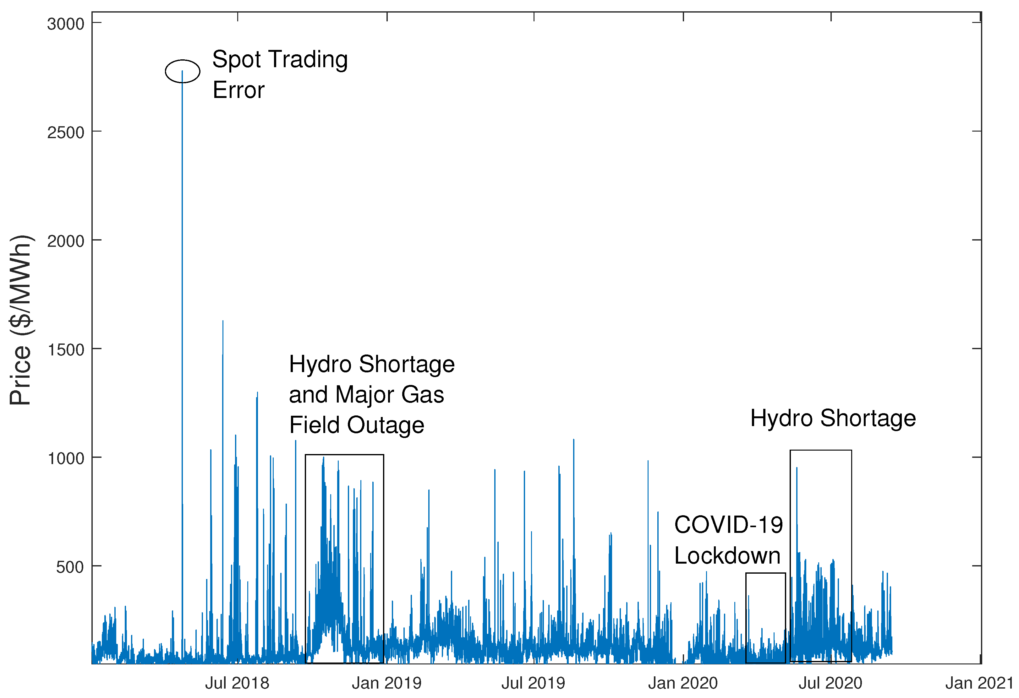
3.1. Description and Key Features

Our electricity price dataset consists of half-hourly electricity prices from the Otahuhu node in New Zealand from 1 January 2018, to 30 September 2020. The New Zealand electricity market is a real-time market, where electricity prices are determined by matching demand and supply every five minutes. The prices are determined as the highest bids made by electricity generators capable of clearing all demand. However, the five-minute prices are not accessible and are averaged to produce the half-hourly prices, which are made publicly available for analysis.

Figure 1 displays the electricity price time series. It is clear from this figure that half-hourly prices exhibit several key characteristics; extreme volatility, upward spikes, and mean-reversion. The figure also shows the impact of several key events. A consistent hydro shortage, due to a lack of rainfall in nearby regions, can significantly increase electricity prices until lake levels return to normal. In October 2018, a hydro shortage, with an unexpected outage in the largest gas field in New Zealand, saw prices consistently around $500/MWh.

Figure 1. Half-hour electricity prices from Otahuhu node in New Zealand.

Figure 2a displays the autocorrelation of our price time series. The cyclical peaks that occur at lags of multiples of 48 indicate the intra-day seasonality behaviour. Since prices are largely influenced by demand, lower demand periods at night-time exhibit lower prices than during day-time. The intra-day seasonality can be further observed in Figure 2b, which displays the mean prices for every half-hour period in our dataset. This figure is a good depiction of the intra-day seasonality behaviour of electricity prices. There are two peaks during the day, the first at approximately 9:00 am as businesses open, and the second around 7:00 pm as residential demand increases. There is a large drop-off thereafter, as demand subsides during late hours. For forecasting purposes, we separate our price time series into four distinct periods; the morning peak from 7:00 am to 11:00 am, the evening peak from 6:00 pm to 10:00 pm, the midday off-peak from 11:00 am to 6:00 pm, and the night off-peak from 10:00 pm to 7:00 am. Figure 3 below provides our reasoning to make this distinction.

Figure 2. Price auto−correlation and average price per trading period. (a) Auto−correlation of half−hourly prices. (b) Average price for each half−hour trading period.

Figure 3. Box plot of prices for each trading period.

Figure 3 displays a box plot of half-hourly electricity prices for our sample period. The bottom and top edges of the box represents the 25th and 75th percentiles of data, while the red line inside the box represents the median price. The red crosses outside the box represents any outliers. Electricity prices exhibit a large quantity of outliers in the form of spikes that are observed in Figure 1. Furthermore, the size and intensity of the outliers are increased during peak price hours. As a result, the peak hours forecasts will have a higher priority than off-peak forecasts.

Our external market data consists of half-hourly demand for electricity in the North Island of New Zealand and several hourly weather variables including temperature, rainfall, air pressure, humidity, solar radiation, wind speed, and wind direction. Weather data are observed from the Auckland International Airport weather station by MetService. Table 1 presents descriptive statistics of price, demand, and weather variables.

Table 1. Descriptive statistics of variables.

	Mean	Median	Variance	Skewness	Kurtosis
Price (NZ$/MWh)	117.67	98.90	8331.90	4.32	52.20
Demand (MWh)	1437.73	1463.03	92,283.67	0.03	2.18
Temperature (Celsius)	15.71	15.50	18.64	0.11	2.63
Rainfall (mm)	0.13	0.00	0.55	17.97	701.54
Solar Radiation (mJ/m2)	172.45	1.00	6938.61	1.58	4.60
Air Pressure (hPa)	1015.80	1016.50	62.59	−0.37	3.29
Humidity (%)	80.47	82.00	146.51	−0.45	2.45
Wind Speed (km/h)	15.88	15.00	95.67	0.77	3.38
Wind Direction (degrees)	180.59	210	10,022.77	−0.22	2.01

In this study, all variables are log-transformed to reduce the impact of outliers and to improve the normality of the data. Furthermore, the wind direction variables is first transformed using a sine transformation to emphasize its cyclical nature.

Table 2 presents the correlation coefficients between price and external variable time series. For the purpose of computing these correlations, we have taken the mean of half-hourly prices and the sum of half-hourly demand to convert them to hourly variables. We can observe instances where some weather variables have a strong correlation among each other, such as temperature and solar radiation, or wind speed and humidity. Regardless, we accept them as explanatory variables and later perform variable-selection techniques using the LASSO and random subspace methods in an effort to remove less significant explanatory variables and improve price forecasts.

Table 2. Correlation coefficient table.

	Price	Demand	Temp	Rain	Solar	Pressure	Humidity	Wind Speed	Wind Direction
Price	1	0.344	−0.0479	0.022	0.108	0.0986	−0.084	0.033	−0.056
Demand	0.344	1	−0.076	0.026	0.246	−0.022	−0.212	0.154	0.061
Temp	−0.0479	−0.076	1	−0.029	0.493	−0.083	−0.464	0.254	−0.021
Rain	0.022	0.026	−0.029	1	−0.073	−0.177	0.166	0.080	0.027
Solar	0.108	0.246	0.493	−0.073	1	0.033	−0.627	0.273	0.093
Pressure	0.0986	−0.022	−0.083	−0.177	0.033	1	−0.084	−0.378	−0.197
Humidity	−0.084	−0.212	−0.464	0.166	−0.627	−0.084	1	−0.412	−0.150
Wind Speed	0.033	0.154	0.254	0.080	0.273	−0.378	−0.412	1	0.166
Wind Direction	−0.056	0.061	−0.021	0.027	0.093	−0.197	−0.150	0.166	1

3.2. Forecast Results

In this section, we present the out-of-sample forecasting results for the various models and methods we have employed in this paper. We also separate the results for peak and off-peak periods. Since electricity prices behave much more erratically during peak periods, the peak forecast metrics are more relevant to our study than off-peak forecasts. We consider the mean absolute deviation (MAD), root mean squared errors (RMSE), and mean absolute percentage errors (MAPE) as forecast metrics. Our estimation data set consists of price, demand, and weather data from 1 January 2018, to 31 December 2019. We only consider data starting from 1 January 2018, because there has been a significant fundamental change in the behavior of the New Zealand electricity market beyond this time period, due to the ban of offshore oil and gas exploration, as well as major outages in significant gas fields in New Zealand. The year 2018 was a transitional period into a more renewable environment for the New Zealand electricity market, and a major step towards a fully renewable scheme. Our forecasting period is from 1 January 2020, to 30 September 2020. During the course of our work, global markets were impacted by the COVID-19 pandemic. However, the impact of COVID-19 on New Zealand electricity prices was minimal. We notice a period in April 2020, during the lockdown in New Zealand, where prices are lower than usual. The lockdown reduced nationwide industrial demand for electricity, as the majority of businesses were closed for this period. Other than this, there are no significant effects of the pandemic on electricity price itself, regardless of the impact on other aspects of the electricity market.

In particular, we conduct two separate studies. The first is a simple, single nine-month out-of sample forecast for the period from 1 January 2020 to 30 September 2020. This forecast is used to assess the long-term capabilities of the models. A second study incorporates a cross-validation scheme of several one-week forecasts, for the same time period. The purpose of this is to compare the short-term capabilities of the models. Even if long-term forecasting is challenging, near-term electricity price forecasts can provide significant practical benefits. These forecasts are crucial for real-time market operations, scheduling of maintenance, storage deployment, demand-side management, and financial trading. For this study, we perform a rolling estimation technique, so parameters are updated after every week. In the single out-of-sample nine-month forecast, we use forecasts of external variables as inputs, whereas in the cross-validation scheme, we use the realized values. In this way, we assure that no future information is used to make price forecasts. The forecast horizons used in this study are common practice in the industry.

Figure 4 shows the actual price density alongside the simulated densities from the MF-VAR and RU-MIDAS-VAR models. We observe that the MF-VAR can capture the lower and upper tails of empirical prices particularly well, however the mid portion of the density curve is not well-matched. On the other hand, the RU-MIDAS-VAR density finds a middle ground between actual and MF-VAR simulated median prices, however its tail approximations are worse than the MF-VAR model.

Figure 4. Density plots of actual and simulated price.

Figure 5 displays the actual electricity price along with simulations generated from the MF-VAR and RU-MIDAS-VAR models. When running multiple simulations, we found that some spikes persistently appear in specific periods in our forecast horizon, suggesting that the weather variables have some impact on price spiking. However, we notice, in several periods, a large mismatch between simulated prices and actual prices. As we expected, there is a vast amount of information in the price data that cannot be explained by weather variables alone. The VAR framework with weather data is capable of capturing key characteristics, however, more data on market dynamics as well as macroeconomic variables, such as commodity prices, may improve our forecasts. Furthermore, we may be able to improve the simulated price density using heavy-tailed distribution within the VAR framework.

Figure 5. Simulations of actual and model prices.

To study the capability of our forecasting models to replicate the mean-reversion and seasonality characteristics of electricity prices, we observe the half-life, and spectral density plots, respectively. The half-life values are derived from the lag 1 autocorrelation coefficient, and they denote the decaying rate of deviations from the long-term mean. Similar half-life values between different time-series’ indicate similar mean-reversion characteristics. Table 3 displays the AR(1) coefficient and corresponding half-life values for the actual prices and prices simulated from the MF-VAR and RU-MIDAS-VAR models with OLS estimates. The half-life is approximately 0.7 for all three time-series, indicating similar mean-reversion rates. The spectral density will show the distribution of variance for each frequency component in the time series. Peaks in the spectral density correspond to dominant frequencies, which are related to seasonality. Visualizing the spectral density plots and observing the correlation of the spectral densities between actual and simulated prices can help us identify the captured seasonality of the models. This visualization is provided in Figure 6. In this figure, we observe the logarithm of power spectral density to improve interpretability. We notice that the spectral density plots of actual and simulated prices are similar, indicating that the models are able to capture the seasonality of electricity prices. Furthermore, the correlation between the spectral densities of actual prices and the MF-VAR simulated price is 0.999, and the correlation between the spectral densities of actual prices and the RU-MIDAS-VAR simulated price is 0.997.

Table 3. Half-life values.

Model	AR(1) Coef.	Half-Life
Actual	−0.9707	0.7140
MF-VAR	−0.9745	0.7113
RU-MIDAS-VAR	−0.9899	0.7002

Figure 6. Spectral density plots of actual and simulated prices.

In Table 3, Table 4, Table 5, Table 6 and Table 7, MLS, MFVB, and GS refer to the multivariate least-squares, mean-field variational Bayes, and Gibbs sampling techniques, respectively. Table 4 shows the out-of-sample forecast results for the models and methods employed in this study. For Bayesian estimation, our experiment uses 100,000 iterations to obtain parameter estimates, where the first 10,000 samples are burned. We also perform thinning by selecting every fifth sample. From the remaining samples, we use the arithmetic mean to obtain parameter estimates, which are then used for forecasting purposes. The left table considers a model with lags of $p=24$ for each variable, whereas the right table shows results for lags of $p=240$. For most estimation methods, the lower lag model performs better. The LASSO method performs significantly better for $p=240$. Comparing the least-squares estimated for the MF-VAR and RU-MIDAS-VAR models, we observe that the MF-VAR model performs marginally better for both lag values. The MFVB and Gibbs sampler estimates are also similar to the least-squares estimates, with the Gibbs sampler performing better in terms of MAPE. The subset regression and projection regression methods provide better forecasts than least-squares for $p=240$, but significantly underperform for $p=24$.

Table 4. Out-of-sample nine-month forecast results. Note: Bold font indicates best result.

	Lag p $=24$				Lag p $=240$
Model	MAD	RMSE	MAPE	Model	MAD	RMSE	MAPE
MF-VAR MLS	45.9472	72.2045	34.6090	MF-VAR MLS	58.9771	87.7004	38.2073
MF-VAR MFVB	46.9001	73.4641	35.2611	MF-VAR MFVB	58.3423	86.4735	37.7803
MF-VAR GS	47.7419	75.9605	30.4006	MF-VAR GS	58.4798	87.5852	35.5844
MF-VAR LASSO				MF-VAR LASSO
$\lambda =0.017200$	42.7937	72.6223	38.3311	$\lambda =0.033160$	44.9211	73.1058	39.1370
$\lambda =0.000180$	45.9872	72.4249	36.1998	$\lambda =0.008214$	57.3355	88.9184	18.5820
Adaptive LASSO	43.1545	70.4230	41.2096	Adaptive LASSO	46.0301	76.0408	29.9470
Subset Regression	54.6850	83.2752	56.9606	Subset Regression	57.2314	86.9146	40.8667
Projection Regression	51.4763	80.8129	53.9186	Projection Regression	55.5147	85.4771	38.6816
RU-MIDAS-VAR MLS	46.0136	72.2729	34.5711	RU-MIDAS-VAR MLS	59.0786	87.8343	38.3589
RU-MIDAS-VAR LASSO				RU-MIDAS-VAR LASSO
$\lambda =0.009849$	42.6590	72.3683	37.9954	$\lambda =0.018975$	45.3994	75.5241	36.6278
$\lambda =0.000078$	46.0803	72.5578	35.9015	$\lambda =0.006214$	58.7990	90.1122	17.6100
Adaptive LASSO	43.5719	71.8944	38.4876	Adaptive LASSO	45.5970	75.8669	38.7187
Subset Regression	52.4915	81.7978	56.3428	Subset Regression	57.7477	87.2958	42.0268
Projection Regression	51.2251	80.8534	53.9446	Projection Regression	55.9291	85.9688	39.3641

Table 5. Out-of-sample forecasts for peak and off-peak time periods for lag $p=24$. Note: Bold font indicates best result.

	Morning Peak				Midday Off-Peak
Model	MAD	RMSE	MAPE	Model	MAD	RMSE	MAPE
MF-VAR MLS	54.6073	82.1370	14.8220	MF-VAR MLS	47.5784	73.1042	3.7002
MF-VAR MFVB	55.3793	83.5628	15.7624	MF-VAR MFVB	48.8180	74.6297	3.9611
MF-VAR GS	55.2612	86.3424	13.2280	MF-VAR GS	48.3737	76.4844	3.2597
MF-VAR LASSO				MF-VAR LASSO
$\lambda =0.002223$	54.6468	82.5341	15.6724	$\lambda =0.018890$	44.0121	73.1371	3.9950
$\lambda =0.013020$	55.0219	89.1511	13.1186	$\lambda =0.013020$	44.2649	72.8327	3.7915
Adaptive LASSO	53.8210	83.2561	15.5626	Adaptive LASSO	45.3429	72.9665	3.9627
Subset Regression	68.3809	101.3910	20.0747	Subset Regression	57.0204	85.4541	5.8694
Projection Regression	65.5759	98.7949	19.5033	Projection Regression	53.1245	82.0871	5.6827
RU-MIDAS-VAR MLS	54.7064	82.2539	14.7734	RU-MIDAS-VAR MLS	47.6310	73.1516	3.6902
RU-MIDAS-VAR LASSO				RU-MIDAS-VAR LASSO
$\lambda =0.001056$	55.0073	82.9469	15.7267	$\lambda =0.013020$	47.6601	73.6399	3.9032
$\lambda =0.000078$	55.0474	82.9350	15.5213	$\lambda =0.017212$	47.6984	75.8949	3.9001
Adaptive LASSO	53.5300	83.7917	14.9882	Adaptive LASSO	44.1214	72.9532	3.8927
Subset Regression	66.7269	100.1605	19.4789	Subset Regression	54.4827	83.5487	5.7332
Projection Regression	65.5392	99.1871	19.1159	Projection Regression	52.6773	81.7077	5.7334
	Evening Peak				Night Off-Peak
Model	MAD	RMSE	MAPE	Model	MAD	RMSE	MAPE
MF-VAR MLS	61.1290	104.7811	0.8279	MF-VAR MLS	39.6659	59.4733	66.3977
MF-VAR MFVB	62.2437	106.5511	0.8689	MF-VAR MFVB	40.4225	60.3357	67.3719
MF-VAR GS	64.7439	110.7438	0.7590	MF-VAR GS	41.9589	62.7301	58.2653
MF-VAR LASSO				MF-VAR LASSO
$\lambda =0.014290$	60.7020	104.8512	0.7521	$\lambda =0.020732$	35.2874	57.2525	76.4216
$\lambda =0.013020$	60.7203	107.1022	0.7467	$\lambda =0.000078$	39.5438	59.4261	68.3569
Adaptive LASSO	56.8763	98.7281	0.8817	Adaptive LASSO	35.4375	59.0505	79.9593
Subset Regression	72.7502	116.9132	1.1265	Subset Regression	46.7055	68.4308	115.0509
Projection Regression	71.8114	116.6687	1.0519	Projection Regression	44.1571	65.8535	105.5108
RU-MIDAS-VAR MLS	61.1883	104.8416	0.8257	RU-MIDAS-VAR MLS	39.7358	59.5502	66.3361
RU-MIDAS-VAR LASSO				RU-MIDAS-VAR LASSO
$\lambda =0.000417$	61.1077	105.2518	0.8456	$\lambda =0.009849$	39.2643	59.4555	74.0237
$\lambda =0.006789$	61.1593	105.4274	0.8437	$\lambda =0.000078$	39.5477	59.4938	68.7988
Adaptive LASSO	56.4591	99.9185	0.8355	Adaptive LASSO	35.2920	59.9381	74.6538
Subset Regression	71.3481	115.9424	1.0911	Subset Regression	43.9589	65.5341	109.3512
Projection Regression	70.8592	116.2536	1.0469	Projection Regression	42.8587	64.8399	104.4356

Table 6. Out-of-sample forecasts for peak and off-peaks time periods for lag $p=240$. Note: Bold font indicates best result.

	Morning Peak				Midday Off-Peak
Model	MAD	RMSE	MAPE	Model	MAD	RMSE	MAPE
MF-VAR MLS	67.9381	97.6032	23.2370	MF-VAR MLS	66.3473	95.4826	8.7707
MF-VAR MFVB	67.2869	96.2480	22.8303	MF-VAR MFVB	65.6230	94.0924	8.5966
MF-VAR GS	67.6195	97.9506	20.3349	MF-VAR GS	65.0256	95.9446	8.1388
MF-VAR LASSO				MF-VAR LASSO
$\lambda =0.002690$	55.6432	80.1613	20.3435	$\lambda =0.033160$	47.2202	77.4684	4.0638
$\lambda =0.009894$	68.8604	105.0660	8.8490	$\lambda =0.009015$	61.6604	93.4404	2.6254
Adaptive LASSO	57.1686	86.5855	14.0758	Adaptive LASSO	49.0756	79.2626	3.4859
Subset Regression	73.6302	106.0827	15.5964	Subset Regression	63.9974	93.0562	5.9785
Projection Regression	72.9490	105.5436	16.2854	Projection Regression	59.8845	89.7752	5.1609
RU-MIDAS-VAR MLS	68.0862	97.7560	23.3134	RU-MIDAS-VAR MLS	66.5073	95.6890	8.7869
RU-MIDAS-VAR LASSO				RU-MIDAS-VAR LASSO
$\lambda =0.039941$	63.9649	94.3260	27.8201	$\lambda =0.036393$	65.9945	97.8141	9.3677
$\lambda =0.001689$	66.5887	95.8687	25.8593	$\lambda =0.000459$	67.1229	98.2629	9.3552
Adaptive LASSO	60.7567	96.0937	13.0557	Adaptive LASSO	48.1070	78.5502	4.0298
Subset Regression	75.2452	107.3810	17.4752	Subset Regression	63.0006	92.2766	5.5519
Projection Regression	72.7223	105.2908	16.3465	Projection Regression	59.7987	89.6835	5.2760
	Evening Peak				Night Off-Peak
Model	MAD	RMSE	MAPE	Model	MAD	RMSE	MAPE
MF-VAR MLS	78.9431	118.5856	2.0710	MF-VAR MLS	47.8377	70.5075	68.4979
MF-VAR MFVB	78.0582	116.9086	2.0301	MF-VAR MFVB	47.3563	69.5981	67.8214
MF-VAR GS	79.1230	117.0852	1.9854	MF-VAR GS	47.7414	70.3040	63.3899
MF-VAR LASSO				MF-VAR LASSO
$\lambda =0.036393$	61.3004	98.0360	0.8575	$\lambda =0.033160$	36.5449	57.2421	75.9995
$\lambda =0.013079$	70.9618	114.9250	0.7219	$\lambda =0.007484$	46.5724	69.6286	34.7978
Adaptive LASSO	59.4086	97.0294	0.9291	Adaptive LASSO	37.2777	58.7348	57.6482
Subset Regression	80.9618	122.4441	1.1081	Subset Regression	45.2735	67.4052	78.2747
Projection Regression	80.9158	123.0694	1.0370	Projection Regression	44.2874	66.7439	75.8000
RU-MIDAS-VAR MLS	79.0620	118.7199	2.0788	RU-MIDAS-VAR MLS	47.8871	70.5774	68.7853
RU-MIDAS-VAR LASSO				RU-MIDAS-VAR LASSO
$\lambda =0.036393$	75.1225	114.8347	2.1224	$\lambda =0.015754$	43.1750	65.0516	68.3824
$\lambda =0.030214$	75.2718	114.9091	2.1174	$\lambda =0.006214$	45.0147	67.2977	39.9329
Adaptive LASSO	62.8122	108.2875	0.8411	Adaptive LASSO	36.8866	58.5351	75.1392
Subset Regression	80.9481	122.6194	1.1255	Subset Regression	45.4298	67.5162	80.0261
Projection Regression	80.9835	123.1973	1.0391	Projection Regression	44.2645	66.7739	74.9143

Table 7. Diebold-Mariano test for comparing similarity in forecasts with different models. Note: Bold font indicates failure to reject the null hypothesis of no difference between forecasts with significance level $\alpha =0.05$.

		MF-VAR							RU-MIDAS-VAR
		MLS	MFVB	GS	LASSO	Adaptive LASSO	Subset Regression	Projection Regression	MLS	LASSO	Adaptive LASSO	Subset Regression	Projection Regression
MF- VAR	MLS	1	2.906	3.053	2.947	3.012	2.244	2.060	0.746	2.894	2.964	2.448	2.289
	MFVB	2.906	1	−1.960	−0.401	−0.433	3.134	3.959	−3.400	0.142	0.358	−2.506	−2.964
	GS	3.053	−1.960	1	0.413	0.561	3.299	3.969	−3.546	−1.808	−2.546	−2.851	−3.110
	LASSO	2.947	−0.401	0.413	1	0.138	4.039	3.776	−3.326	−0.381	−0.391	−4.081	−3.612
	Adaptive LASSO	3.012	−0.433	0.561	0.138	1	4.039	3.665	−3.566	−0.543	−0.278	−3.595	−3.426
	Subset Regression	2.244	3.134	3.299	4.039	4.039	1	−1.893	−2.341	3.277	3.619	0.767	3.565
	Projection Regression	2.060	3.959	3.969	3.776	3.665	−1.893	1	−2.060	3.957	4.287	2.755	2.229
RU- MIDAS- VAR	MLS	0.746	−3.400	−3.546	−3.326	−3.566	−2.341	−2.060	1	3.396	3.762	2.627	2.403
	LASSO	2.894	0.142	−1.808	−0.381	−0.543	3.277	3.957	3.396	1	−0.394	2.743	2.990
	Adaptive LASSO	2.964	0.358	−2.546	−0.391	−0.278	3.619	4.287	3.762	−0.394	1	2.493	3.118
	Subset Regression	2.448	−2.506	−2.851	−4.081	−3.595	0.767	2.755	2.627	2.743	2.493	1	−1.912
	Projection Regression	2.289	−2.964	−3.110	−3.612	−3.426	3.565	2.229	2.403	2.990	3.118	−1.912	1

We provide two LASSO estimates with different $\lambda$ values so we may study their optimal performance for all forecast metrics. Generally, the LASSO results are similar for both $p=24$ and $p=240$, since, for the latter case, the LASSO likely removes any insignificant, higher lag data. We also notice that, for $p=240$, the LASSO identifies a parameter set that significantly reduces the MAPE compared to other methods. In particular, we find that the LASSO chosen coefficients include recent price, demand, and solar energy values. Wind speed and wind direction of beyond lag 10 are also relevant, indicating a delayed effect of wind power. Less prominent, but still included features are recent rainfall and humidity values. We find air pressure to hold no important information and it is mostly excluded in the parameter set. Furthermore, for the study of 240 lags, we find that price, demand, wind metrics, and rainfall can have hold information about current prices even beyond a week. However, solar, humidity, and air pressure do not hold significant information beyond the previous day. This means that all the significant variables play an important role in electricity price forecasting. Hence, accurate forecasts of these variables will also affect the accuracy of electricity price forecasts. Nevertheless, weather forecasts are beyond the scope of this study.

Table 5 and Table 6 separate the results of Table 4 into peak and off-peak forecasts for $p=24$ and $p=240$, respectively. From prior analysis, it is clear that electricity prices exhibit larger volatility and more spike frequencies during peak periods. This is a direct result of higher demand and significant generation costs during peak periods. This also necessitates a larger focus on forecasting capabilities for peak periods, since there is much more risk involved for generators and retailers of electricity during these periods. Therefore, we would like to examine the peak period forecasting capabilities of our models. We notice that the forecasts are much better for the off-peak periods than the peak periods. We expected this since the peak periods exhibit much higher volatility and frequency of spikes. In general, the LASSO and adaptive LASSO models perform significantly better than the other methods, especially so in Table 6 for $p=240$, where the MF-VAR LASSO significantly outperforms even the RU-MIDAS-VAR LASSO model. Again, the MF-VAR and RU-MIDAS-VAR least-squares estimates provide similar results, with the MF-VAR performing slightly better. An interesting result is that the MAPE for evening peaks is significantly lower than other periods of the day, despite the MAD and RMSE being higher. The reason for this is the MAPE has a more severe penalty for negative errors and the models are consistently overestimating evening prices. Finally, Table 8 displays the out-of-sample cross-validation results for rolling 1-week periods. We further separate cross-validation results into peak and off-peak periods. Note that, in some cases, only a single LASSO value is shown, since the LASSO value obtains the best result for every forecast metric. The forecast performance of the models relative to each other in the cross-validation context is similar to the fixed-window nine-month forecast, suggesting that our results are robust to changes in the forecast horizon. The raw values in cross-validation are lower than their nine-month forecast counterparts in Table 4, Table 5 and Table 6, since the former produces one-week forecasts while the latter produces a nine-month forecast. As suggested by a reviewer, technological factors of energy generation from different renewable sources may have a significant impact on electricity prices but we leave this for future research.

Table 8. One-week cross-validation results for lags $p=24$ (left) and $p=240$ (right). Note: Bold font indicates best result.

	Lag p = 24				Lag p = 240
Overall Cross-Validation
Model	MAD	RMSE	MAPE	Model	MAD	RMSE	MAPE
MF-VAR MLS	39.0213	54.2849	25.9527	MF-VAR MLS	43.9939	59.8975	20.7390
MF-VAR MFVB	39.0588	54.4013	26.0758	MF-VAR MFVB	43.9310	59.9331	20.9073
MF-VAR GS	39.0699	54.3874	25.7957	MF-VAR GS	44.4511	60.4291	20.4364
MF-VAR LASSO				MF-VAR LASSO
$\lambda =0.000213$	39.3532	54.6452	26.5770	$\lambda =0.003174$	39.1645	55.5124	19.0060
$\lambda =0.000092$	39.4099	54.6039	26.0981	$\lambda =0.001374$	40.1439	55.9094	18.3995
Adaptive LASSO	39.5322	55.4278	26.5786	Adaptive LASSO	39.5543	55.9071	19.6482
Subset Regression	45.1129	64.4887	48.1684	Subset Regression	43.3860	61.8194	20.8003
Projection Regression	43.9946	63.5313	46.1500	Projection Regression	43.1366	61.7508	20.5415
RU-MIDAS-VAR MLS	39.0448	54.2908	25.9188	RU-MIDAS-VAR MLS	43.9905	59.8949	20.6971
RU-MIDAS-VAR LASSO				RU-MIDAS-VAR LASSO
$\lambda =0.000092$	39.0548	54.4545	27.0251	$\lambda =0.001817$	39.7438	56.0688	19.8824
-	-	-	-	$\lambda =0.000653$	40.8673	56.5273	19.2821
Adaptive LASSO	39.5127	55.5343	26.6036	Adaptive LASSO	40.0017	55.9823	19.6184
Subset Regression	44.5340	63.9418	47.6400	Subset Regression	43.2785	61.8100	20.7348
Projection Regression	44.1214	63.5890	46.2788	Projection Regression	43.2121	61.7507	20.8290
Morning Peak Cross-Validation
Model	MAD	RMSE	MAPE	Model	MAD	RMSE	MAPE
MF-VAR MLS	43.8639	58.2397	10.0080	MF-VAR MLS	51.0876	65.7240	8.1383
MF-VAR MFVB	43.9907	58.2995	10.3847	MF-VAR MFVB	50.7665	65.5618	8.4403
MF-VAR GS	44.0088	58.5488	9.8737	MF-VAR GS	51.5391	66.3977	7.2382
MF-VAR LASSO				MF-VAR LASSO
$\lambda =0.000092$	44.7242	59.1166	10.4724	$\lambda =0.002188$	46.2319	60.9060	7.5837
-	-	-	-	$\lambda =0.014065$	52.3180	68.4850	5.4996
Adaptive LASSO	43.8443	59.0427	10.0107	Adaptive LASSO	47.0004	60.5723	6.2794
Subset Regression	57.2532	73.8674	13.1330	Subset Regression	55.0560	71.3817	11.0370
Projection Regression	57.8610	74.6463	12.5676	Projection Regression	55.4509	71.7095	11.2152
RU-MIDAS-VAR MLS	43.8844	58.2552	9.9796	RU-MIDAS-VAR MLS	51.0863	65.7137	8.0282
RU-MIDAS-VAR LASSO				RU-MIDAS-VAR LASSO
$\lambda =0.000092$	44.3937	58.9833	10.3828	$\lambda =0.000947$	46.9679	61.5296	8.2155
-	-	-	-	$\lambda =0.009694$	53.0959	69.4049	5.1654
Adaptive LASSO	44.0027	59.4278	11.8893	Adaptive LASSO	47.4248	61.1734	6.2672
Subset Regression	56.6396	73.3442	12.7472	Subset Regression	55.5680	71.8681	11.5234
Projection Regression	56.1396	72.9728	13.0419	Projection Regression	55.4070	71.6640	11.7774
Evening Peak Cross-Validation
Model	MAD	RMSE	MAPE	Model	MAD	RMSE	MAPE
MF-VAR MLS	52.7036	69.5604	0.6461	MF-VAR MLS	55.7896	73.6556	0.8524
MF-VAR MFVB	52.6321	69.4464	0.6617	MF-VAR MFVB	55.9292	73.8143	0.8721
MF-VAR GS	52.7788	69.7454	0.6286	MF-VAR GS	56.5841	74.1283	0.8266
MF-VAR LASSO				MF-VAR LASSO
$\lambda =0.000194$	52.5444	69.6440	0.6617	$\lambda =0.004196$	49.8996	68.4681	0.6113
$\lambda =0.000092$	52.6011	69.6018	0.6581	$\lambda =0.015436$	53.1975	72.7117	0.5464
Adaptive LASSO	52.6772	69.7427	0.6613	Adaptive LASSO	49.8631	68.3418	0.5994
Subset Regression	61.8930	81.6559	0.8904	Subset Regression	53.5917	73.3821	0.9414
Projection Regression	61.0245	80.6504	0.8715	Projection Regression	54.4470	74.4293	0.9545
RU-MIDAS-VAR MLS	52.7315	69.5781	0.6460	RU-MIDAS-VAR MLS	55.7557	73.6337	0.8530
RU-MIDAS-VAR LASSO				RU-MIDAS-VAR LASSO
$\lambda =0.000234$	52.5322	69.7340	0.6729	$\lambda =0.001817$	51.0066	68.5294	0.7254
$\lambda =0.000101$	52.6387	69.7206	0.6629	$\lambda =0.010640$	53.2158	72.8385	0.5546
Adaptive LASSO	52.5016	69.5445	0.6602	Adaptive LASSO	51.0101	68.5017	0.6478
Subset Regression	61.1652	81.0363	0.8681	Subset Regression	54.1344	73.7514	0.9815
Projection Regression	61.6345	81.4736	0.8602	Projection Regression	54.1406	73.7965	0.9665
Afternoon Off-Peak Cross-Validation
Model	MAD	RMSE	MAPE	Model	MAD	RMSE	MAPE
MF-VAR MLS	39.8537	54.4063	2.9195	MF-VAR MLS	47.5721	62.9285	2.9189
MF-VAR MFVB	39.7880	54.4804	3.0612	MF-VAR MFVB	47.4596	63.0013	3.0012
MF-VAR GS	39.9843	54.6214	2.8014	MF-VAR GS	48.3398	64.0571	2.7732
MF-VAR LASSO				MF-VAR LASSO
$\lambda =0.000092$	40.7583	54.9285	3.0502	$\lambda =0.039136$	42.2081	60.2456	2.4681
-	-	-	-	$\lambda =0.011677$	43.9839	60.0132	1.9250
Adaptive LASSO	40.8676	56.0234	2.9358	Adaptive LASSO	43.0138	60.3792	2.3438
Subset Regression	45.7822	63.7576	4.2465	Subset Regression	45.8491	63.8941	3.5062
Projection Regression	44.6630	62.6429	4.3299	Projection Regression	45.7327	63.5678	3.5471
RU-MIDAS-VAR MLS	39.8304	54.3609	2.9204	RU-MIDAS-VAR MLS	47.5807	62.9313	2.9191
RU-MIDAS-VAR LASSO				RU-MIDAS-VAR LASSO
$\lambda =0.000092$	40.2548	54.7857	3.0817	$\lambda =0.026975$	42.6140	61.0330	2.5166
-	-	-	-	$\lambda =0.004196$	42.7366	58.9088	2.0225
Adaptive LASSO	40.5783	54.3715	3.0957	Adaptive LASSO	42.5791	61.5725	2.4816
Subset Regression	45.0336	63.1032	4.2150	Subset Regression	45.7977	63.8068	3.5176
Projection Regression	44.3662	62.3619	4.3749	Projection Regression	45.6615	63.6501	3.4872
Night Off-Peak Cross-Validation
Model	MAD	RMSE	MAPE	Model	MAD	RMSE	MAPE
MF-VAR MLS	33.3966	44.9116	49.5500	MF-VAR MLS	36.3687	48.4260	39.1064
MF-VAR MFVB	33.5049	45.0345	49.6254	MF-VAR MFVB	36.3521	48.4165	39.3302
MF-VAR GS	33.3630	44.8812	49.3355	MF-VAR GS	36.5378	48.5702	38.7799
MF-VAR LASSO				MF-VAR LASSO
$\lambda =0.018521$	32.3393	46.0774	68.6164	$\lambda =0.003174$	32.0412	44.2983	36.0362
$\lambda =0.000372$	33.1203	44.8136	51.7147	$\lambda =0.001374$	32.5423	44.5084	34.5579
Adaptive LASSO	33.1236	45.9539	52.0444	Adaptive LASSO	32.2955	44.6052	35.7815
Subset Regression	37.1682	51.9024	94.5028	Subset Regression	35.6758	49.3582	36.3426
Projection Regression	37.4977	52.3368	95.8479	Projection Regression	35.5013	49.1460	38.0939
RU-MIDAS-VAR MLS	33.4498	44.9400	49.4855	RU-MIDAS-VAR MLS	36.3638	48.4273	39.0438
RU-MIDAS-VAR LASSO				RU-MIDAS-VAR LASSO
$\lambda =0.012766$	32.2032	45.9315	69.5419	$\lambda =0.024579$	32.1665	45.8040	55.9070
$\lambda =0.000213$	32.9623	44.6521	52.6003	$\lambda =0.000542$	33.5490	45.3027	36.1274
Adaptive LASSO	33.0932	46.0954	53.1199	Adaptive LASSO	32.3220	45.3433	39.8832
Subset Regression	36.7217	51.4238	93.0253	Subset Regression	35.4182	49.1436	37.9251
Projection Regression	36.3093	51.1871	90.0338	Projection Regression	35.4040	49.1487	38.0873

Table 7 displays the results of the two-sided Diebold-Mariano (DM) test to compare the predictive accuracy of forecasts from two models for lag $p=240$, see Diebold (2015) for details on the DM test. The null hypothesis of the DM test is that the two forecasts have similar predictive accuracy. Since this is a two-tailed test, a significance level $\alpha =0.05$ suggests that the null hypothesis of no difference in forecasts will be rejected if the computed DM statistics fall outside the range of $-1.96$ to $1.96$. In cases where the forecasts are obtained multiple times, such as in Bayesian inference methods and random subspace methods, the test statistics are computed several times and averaged. We observe from the table that the MFVB, Gibbs sampler, MF-VAR LASSO, and RU-MIDAS-VAR LASSO obtain similar forecasts. This reflects the similarity between the two procedures in that a prior selection in Bayesian inference is a form of regularization. We also observe that the MLS, subset regression, and projection regression forecasts have similar predictions between their MF-VAR and RU-MIDAS-VAR variants, as do the LASSO and adaptive LASSO methods.

We also present the result of the Model Confidence Set (MCS) developed by Hansen et al. (2011). The MCS procedure contains a series of tests to construct a set of superior models, which contains the best model with a given confidence level. The test null hypothesis is that all model’s have equal predictive ability. The test is calculated for a specific loss function, which can be chosen depending on the specific forecasting taqsk. In our study, we choose the loss function to simply be the absolute errors. Furthermore, we conduct the test for a confidence level of $\alpha =0.05$. We have implemented the test using the MFE Toolbox in MATLAB, see Sheppard (2009). The MCS procedure selects the MF-VAR LASSO as the only model in the superior set of models for both lags of $p=24$ and $p=240$, and the corresponding p-value of this test is 2 $\times {10}^{-4}$, indicating that the null hypothesis of equal predictive ability amongst all models is rejected at the 5% level.

4. Conclusions

The aim of this paper was to study the half-hourly electricity price forecasting capability of an MF-VAR model which incorporated weather data and demand. To our knowledge, this paper is the first to study the dynamics of intra-day electricity prices using the MF-VAR framework. Our forecasting results show that incorporating weather data and demand is capable of replicating several key characteristics observed in electricity prices; persistent volatility, spikes, and mean-reversion. Our out-of-sample density plots show that the MF-VAR model captured the lower and upper tails of actual price density well, however, there was a mismatch around median prices. The VAR is a capable framework for electricity price forecasting but additional data relating to market dynamics and macroeconomic factors may improve our forecasting capabilities.

Furthermore, we applied several techniques for estimating an MF-VAR framework. In particular, we used the mean-field variational Bayes as an approximation for Gibbs sampling estimates. Our results were promising and suggested that the MFVB provides impressive approximations to the Gibbs sampler estimates when applied to electricity prices in New Zealand, and within a VAR framework. The MFVB, therefore, proves to be a useful alternative Bayesian tool, particularly for large sets of data and parameters, due to the rapid computational time. In particular, while Gibbs sampling with 100,000 iterations took approximately 45 min, the VB ELBO converged in nearly 30 s, with a convergence threshold of ${10}^{-7}$. This was a significant improvement in computational time, with little different in the forecast results.

We also discussed an alternative mixed-frequency model, the RU-MIDAS model. We showed that easing the error restriction in this model allows us to specify the RU-MIDAS within a VAR framework, and we refer to it as the RU-MIDAS-VAR model. This paper is the first to study this relationship. Furthermore, we show that the RU-MIDAS-VAR closely resembles the MF-VAR, however, it uses more up-to-date information for its lags. Despite this, our forecast results show that the MF-VAR and the RU-MIDAS-VAR provide similar price predictions, with the MF-VAR performing marginally better.

We also incorporate the LASSO, adaptive LASSO, and random subspace methods as variable selection tools for our models. Our forecast results show that the LASSO performs extremely well for both the MF-VAR and RU-MIDAS-VAR models within the New Zealand electricity market. The LASSO and adaptive LASSO outperform all other methods in nearly all metrics, particularly so when a larger parameter set is used. The LASSO also allows us to identify the optimal parameter set for a specific criterion. The random subspace methods as dimension reduction techniques performed better than least-squares estimates for a larger parameter set, however, they did not perform well otherwise. They may still have useful practical applications for studies with large datasets and parameter sets.

We employed a two-sided Diebold-Mariano test on the full set of models. The test showed that the predictions of the MFVB, Gibbs Sampler, MF-VAR LASSO and adaptive LASSO, and RU-MIDAS-VAR LASSO and adaptive LASSO models significantly outperform the other models, however there was not a significant difference in prediction accuracy amongst these models. On the other hand, our results from the Model Confidence Set (MCS) suggested the MF-VAR LASSO as the only model in the superior set of models for both lags $p=24$ and $p=240$.

Finally, we extended our forecasting studies by observing forecasts for specific periods in a day, i.e., peak and off-peak periods. The models generally perform better for off-peak periods, as one would expect, since peak periods exhibit much higher volatility and spike frequency. However, to adjust for this, it may be beneficial to test heavy-tailed distribution such as the generalized Pareto distribution or to incorporate stochastic volatility within a VAR framework. In the future, we hope to extend this study to incorporate more useful electricity market and macroeconomic variables, which may improve price predictions. Another important aspect for future work is to compare electricity price forecasts across markets.

References

- Bańbura, M., Giannone, D., & Reichlin, L. (2010). Large bayesian vector auto regressions. Journal of Applied Econometrics, 25(1), 71–92. [Google Scholar] [CrossRef]
- Bishop, C. M., & Nasrabadi, M. (2006). Pattern recognition and machine learning (Vol. 4). Springer. [Google Scholar]
- Blei, D. M., Kucukelbir, A., & McAuliffe, J. D. (2017). Variational inference: A review for statisticians. Journal of the American Statistical Association, 112(518), 859–877. [Google Scholar] [CrossRef]
- Boot, T., & Nibbering, D. (2019). Forecasting using random subspace methods. Journal of Econometrics, 209(2), 391–406. [Google Scholar] [CrossRef]
- Carvalho, C. M., Polson, N. G., & Scott, J. G. (2010). The horseshoe estimator for sparse signals. Biometrika, 97(2), 465–480. [Google Scholar] [CrossRef]
- Cavalcante, L., Bessa, R. J., Reis, M., & Browell, J. (2017). Lasso vector autoregression structures for very short-term wind power forecasting. Wind Energy, 20(4), 657–675. [Google Scholar] [CrossRef]
- Cross, J. L., Hou, C., & Poon, A. (2020). Macroeconomic forecasting with large bayesian vars: Global-local priors and the illusion of sparsity. International Journal of Forecasting, 36(3), 899–915. [Google Scholar] [CrossRef]
- Diebold, F. X. (2015). Comparing predictive accuracy, twenty years later: A personal perspective on the use and abuse of diebold–mariano tests. Journal of Business & Economic Statistics, 33(1), 1. [Google Scholar]
- Eraker, B., Chiu, C. W., Foerster, A. T., Kim, T. B., & Seoane, H. D. (2014). Bayesian mixed frequency vars. Journal of Financial Econometrics, 13(3), 698–721. [Google Scholar] [CrossRef]
- Foroni, C., Ravazzolo, F., & Rossini, L. (2023). Are low frequency macroeconomic variables important for high frequency electricity prices? Economic Modelling, 120, 106160. [Google Scholar] [CrossRef]
- Gefang, D. (2014). Bayesian doubly adaptive elastic-net lasso for var shrinkage. International Journal of Forecasting, 30(1), 1–11. [Google Scholar] [CrossRef]
- Gefang, D., Koop, G., & Poon, A. (2020). Computationally efficient inference in large bayesian mixed frequency vars. Economics Letters, 191, 109120. [Google Scholar] [CrossRef]
- Gefang, D., Koop, G., & Poon, A. (2023). Forecasting using variational bayesian inference in large vector autoregressions with hierarchical shrinkage. International Journal of Forecasting, 39(1), 346–363. [Google Scholar] [CrossRef]
- Ghysels, E. (2016). Macroeconomics and the reality of mixed frequency data. Journal of Econometrics, 193(2), 294–314. [Google Scholar] [CrossRef]
- Ghysels, E., Santa-Clara, P., & Valkanov, R. (2004). The midas touch: Mixed data sampling regression models. UCLA: Finance. Available online: https://escholarship.org/uc/item/9mf223rs (accessed on 15 July 2022).
- Götz, T. B., & Hauzenberger, K. (2021). Large mixed-frequency vars with a parsimonious time-varying parameter structure. The Econometrics Journal, 24(3), 442–461. [Google Scholar] [CrossRef]
- Hansen, P. R., Lunde, A., & Nason, J. M. (2011). The model confidence set. Econometrica, 79(2), 453–497. [Google Scholar] [CrossRef]
- Hsu, N., Hung, H., & Chang, Y. (2008). Subset selection for vector autoregressive processes using lasso. Computational Statistics & Data Analysis, 52(7), 3645–3657. [Google Scholar]
- Huurman, C., Ravazzolo, F., & Zhou, C. (2012). The power of weather. Computational Statistics & Data Analysis, 56(11), 3793–3807. [Google Scholar]
- Jedrzejewski, A., Marcjasz, G., & Weron, R. (2021). Importance of the long-term seasonal component in day-ahead electricity price forecasting revisited: Parameter-rich models estimated via the lasso. Energies, 14(11), 3249. [Google Scholar] [CrossRef]
- Kapoor, G., & Wichitaksorn, N. (2023). Electricity price forecasting in New Zealand: A comparative analysis of statistical and machine learning models with feature selection. Applied Energy, 347, 121446. [Google Scholar] [CrossRef]
- Koop, G., & Korobilis, D. (2010). Bayesian multivariate time series methods for empirical macroeconomics. Foundations and Trends in Econometrics, 3(4), 267–358. [Google Scholar] [CrossRef]
- Koop, G., & Korobilis, D. (2018). Variational bayes inference in high-dimensional time-varying parameter models. Available online: https://mpra.ub.uni-muenchen.de/id/eprint/87972 (accessed on 1 August 2022).
- Litterman, R. B. (1986). Forecasting with bayesian vector autoregressions—Five years of experience. Journal of Business & Economic Statistics, 4(1), 25–38. [Google Scholar]
- Ludwig, N., Feuerriegel, S., & Neumann, D. (2015). Putting big data analytics to work: Feature selection for forecasting electricity prices using the lasso and random forests. Journal of Decision Systems, 24(1), 19–36. [Google Scholar] [CrossRef]
- Marcjasz, G., Uniejewski, B., & Weron, R. (2020). Beating the naïve—Combining lasso with naïve intraday electricity price forecasts. Energies, 13(7), 1667. [Google Scholar] [CrossRef]
- Messner, J. W., & Pinson, P. (2019). Online adaptive lasso estimation in vector autoregressive models for high dimensional wind power forecasting. International Journal of Forecasting, 35(4), 1485–1498. [Google Scholar] [CrossRef]
- Mosquera-López, S., Uribe, J. M., & Manotas-Duque, D. F. (2017). Nonlinear empirical pricing in electricity markets using fundamental weather factors. Energy, 139, 594–605. [Google Scholar] [CrossRef]
- Ormerod, J. T., & Wand, M. P. (2010). Explaining variational approximations. The American Statistician, 64(2), 140–153. [Google Scholar] [CrossRef]
- Schorfheide, F., & Song, D. (2015). Real-time forecasting with a mixed-frequency var. Journal of Business & Economic Statistics, 33(3), 366–380. [Google Scholar]
- Sheppard, K. (2009). Mfe matlab function reference financial econometrics. Available online: https://www.kevinsheppard.com/files/code/matlab/mfe-toolbox-documentation.pdf (accessed on 22 March 2022).
- Sims, C. A. (1980). Macroeconomics and reality. Econometrica: Journal of the Econometric Society, 48, 1–48. [Google Scholar] [CrossRef]
- Son, H., & Kim, C. (2017). Short-term forecasting of electricity demand for the residential sector using weather and social variables. Resources, Conservation and Recycling, 123, 200–207. [Google Scholar] [CrossRef]
- Suomalainen, K., Pritchard, G., Sharp, B., Yuan, Z., & Zakeri, G. (2015). Correlation analysis on wind and hydro resources with electricity demand and prices in new zealand. Applied Energy, 137, 445–462. [Google Scholar] [CrossRef]
- Tibshirani, R. (1996). Regression shrinkage and selection via the lasso. Journal of the Royal Statistical Society: Series B (Methodological), 58(1), 267–288. [Google Scholar] [CrossRef]
- Uniejewski, B., Marcjasz, G., & Weron, R. (2019). Understanding intraday electricity markets: Variable selection and very short-term price forecasting using lasso. International Journal of Forecasting, 35(4), 1533–1547. [Google Scholar] [CrossRef]
- Uniejewski, B., & Weron, B. (2018). Efficient forecasting of electricity spot prices with expert and lasso models. Energies, 11(8), 2039. [Google Scholar] [CrossRef]
- Wand, M. P., Ormerod, J. T., Padoan, S. A., & Frühwirth, R. (2011). Mean field variational bayes for elaborate distributions. Bayesian Analysis, 6(4), 847–900. [Google Scholar] [CrossRef]
- Weron, R. (2014). Electricity price forecasting: A review of the state-of-the-art with a look into the future. International Journal of Forecasting, 30(4), 1030–1081. [Google Scholar] [CrossRef]
- You, C., Ormerod, J. T., & Mueller, S. (2014). On variational bayes estimation and variational information criteria for linear regression models. Australian & New Zealand Journal of Statistics, 56(1), 73–87. [Google Scholar]
- Ziel, F. (2016). Forecasting electricity spot prices using lasso: On capturing the autoregressive intraday structure. IEEE Transactions on Power Systems, 31(6), 4977–4987. [Google Scholar] [CrossRef]
- Zou, H. (2006). The adaptive lasso and its oracle properties. Journal of the American Statistical Association, 101(476), 1418–1429. [Google Scholar] [CrossRef]
Disclaimer/Publisher’s Note: The statements, opinions and data contained in all publications are solely those of the individual author(s) and contributor(s) and not of MDPI and/or the editor(s). MDPI and/or the editor(s) disclaim responsibility for any injury to people or property resulting from any ideas, methods, instructions or products referred to in the content. |
© 2025 by the authors. Licensee MDPI, Basel, Switzerland. This article is an open access article distributed under the terms and conditions of the Creative Commons Attribution (CC BY) license (https://creativecommons.org/licenses/by/4.0/).