Optimal Time Series Forecasting Through the GARMA Model

Abstract

This paper examines the use of machine learning methods in modeling and forecasting time series with long memory through GARMA. By employing rigorous model selection criteria through simulation study, we find that the hybrid GARMA-LSTM model outperforms traditional approaches in forecasting long-memory time series. This characteristic is confirmed using popular datasets such as sunspot data and Australian beer production data. This approach provides a robust framework for accurate and reliable forecasting in long-memory time series. Additionally, we compare the GARMA-LSTM model with other implemented models, such as GARMA, TBATS, ARIMA, and ANN, highlighting its ability to address both long-memory and non-linear dynamics. Finally, we discuss the representativeness of the datasets selected and the adaptability of the proposed hybrid model to various time series scenarios.

1. Introduction

Time series analysis is a critical field of many scientific studies aiming at the pursuit of enhanced forecasting accuracy. Its significance is notably evident in solar activity and industrial production. For example, solar activity, as represented by sunspot numbers, is vital for understanding long-term climate variations and other natural phenomena. Similarly, in the industrial sector, accurate forecasting of production volumes, such as in the Australian beer production industry, is crucial for effective supply chain management, inventory control, and strategic planning. The complex nature of these time series, characterized by their long-memory and non-linear dynamics, presents substantial challenges to traditional forecasting models (Ao & Fayek, 2023; Bagga, 2023; Cheng et al., 2015; Zohrevand et al., 2017).

Historically, popular linear models formed by the ARIMA (autoregressive integrated moving average) approach have formed the backbone of time series forecasting. However, their limitations in capturing the nuances of these factors have led researchers to explore more advanced models than ARIMA. In light of these advancements, the GARMA model has been recognized; see, for example, Granger and Joyeux (1980), Hosking (1981), and Woodward et al. (1998).

This study combines the GARMA model’s adaptability in handling long memory with LSTM’s capability to learn non-linear dependencies. This approach aims to address the complexities inherent in forecasting time series, specifically sunspot and Australian beer production, by leveraging the strengths of both GARMA and LSTM models. Additionally, we compare the GARMA-LSTM hybrid model with other traditional and advanced models, including GARMA, TBATS, ARIMA, and ANN.

The primary aim of this study is to investigate the predictive ability of the GARMA-LSTM model in the context of sunspot and Australian beer production data. Our investigation focuses on assessing the model’s performance in capturing long-memory processes and non-linear dynamics. We also discuss the relevance of the chosen datasets, highlighting their long-memory and seasonal characteristics, which align well with the proposed model’s strengths.

In developing these models, our approach closely follows the pioneering work of Hochreiter and Schmidhuber (1997), Zhang et al. (1998) and Zhang (2003), which integrates statistical methodologies with neural network algorithms to create hybrid forecasting models. This synthesis aims to harness the strengths of both statistical models and advanced machine learning techniques for superior predictive accuracy; see, for example, Gadhi et al. (2024), Makridakis et al. (2018), Tang et al. (2020), Mosavi et al. (2018), and Ali et al. (2024).

The paper is structured as follows: We begin by detailing the methodological approach, emphasizing the development and implementation of the GARMA-LSTM model. Following this, we present empirical findings, focusing on the model’s efficacy in forecasting sunspot data and Australian beer production. The subsequent section discusses these results considering their implications for time series forecasting, including potential limitations of the hybrid model. Finally, we conclude the paper by reflecting on the significance of these time series findings and future prospects of hybrid modeling.

2. Methodology

This section provides details of time series models and required methods for later reference.

2.1. K-Factor GARMA Model

Suppose that a time series $\left\{X_t\right\}$ is generated by

$$\varphi \left(L\right)\prod _{i=1}^k{(1-2u_{i}L+L^2)}^{d_i}{(1-L)}^d(X_t-\mu )=\theta \left(L\right){\epsilon }_t,$$

(1)

where

(a)

$|u_i|\le 1\mathrm{and}{d}_i\in \left(0,{\displaystyle \frac{1}{2}}\right),i=1,2,\dots ,k$ are real parameters and $d=0,1,2,\dots$.

(b)

$\left\{{\epsilon }_t\right\}$ is a white noise process with zero mean and variance ${\sigma }^2$.

(c)

The zeros of $\varphi \left(L\right)$ and $\theta \left(L\right)$ lie outside the unit circle to ensure the square summability of the coefficients in both ${\left[\varphi \left(L\right)\right]}^{-1}$ and ${\left[\theta \left(L\right)\right]}^{-1}$.

Without loss of generality, set $d=0$ and consider the family general by

$$\varphi \left(L\right)\prod _{i=1}^k{(1-2u_{i}L+L^2)}^{d_i}(X_t-\mu )=\theta \left(L\right){\epsilon }_t.$$

(2)

The family in Equation (2) is known as a univariate k-factor Gegenbauer ARMA of order $(p,d_i,q;u_i)$, or GARMA$(p,d,q;u_i)$. The following regularity conditions will be used in theoretical developments:

AR regularity conditions:

The process in Equation (2) is said to be AR regular if the zeros of $\varphi \left(L\right)$ are outside the unit circle, $|u_i| < 1$ and $d_i<1/2$ or $|u_i| =1$ and $d_i<1/4$.

MA regularity conditions: The process in Equation (2) is said to be MA regular if the zeros of $\theta \left(L\right)$ are outside the unit circle, $|u_i| < 1$ and $d_i>-1/2$ or $|u_i| =1$ and $d_i>-1/4$.

When $k=1$ in (2), the GARMA$(p,d_1,q;u_1)$ becomes $\varphi \left(L\right){(1-2u_{i}L+L^2)}^{d_1}(X_t-\mu )=\theta \left(L\right){\epsilon }_t$ and enjoys the following properties:

• The power spectrum:

  $$f\left(\omega \right)=C{\left[4{(cos\omega -u_1)}^2\right]}^{-d_1},-\pi <\omega <\pi ,$$

  (3)

  where $C={\left|{\displaystyle \frac{\theta \left(e^{-i\omega }\right)}{\varphi \left(e^{-i\omega }\right)}}\right|}^2{\displaystyle \frac{{\sigma }^2}{2\pi }}$ is a constant.

It is clear from (3) that the long memory features are characterized by the unbounded spectrum at

$${\omega }_1={cos}^{-1}\left(u_1\right),$$

when $|u_1| < 1$ and $d_1>0$. The parameter $u_1$ determines the location of the Gegenbauer frequency ${\omega }_1$, which represents the cyclic component of the process. Therefore, (2) is stationary and explains generalized long memory behavior when $|u_1| < 1$ and $0<d_1<1/2$. The frequency ${\omega }_1$ is known as the Gegenbauer frequency.

It is evident that when $u_1=1$, ${\omega }_1=0$, the Equation (2) reduces to a standard long memory ARFIMA model with index $2d_1$ for $0<d_1<1/4$.

In their papers, Dissanayake et al. (2018) and Peiris and Hunt (2023) have discussed these properties in detail. For convenience, set $u_1=u$ and $d_1=d$ with $p=q=0$; below, we consider the GARMA$(0,d,0;u)$.

2.2. Some Basic Results of GARMA$(0,d,0;u)$

Consider the class of GARMA$(0,d,0;u)$ given by

$${(1-2uL+L^2)}^d{X}_t={ϵ}_t.$$

(4)

Under the AR regularity conditions, it is easy to show that the Wold representation of (4) is given by

$$X_t=\psi \left(L\right){ϵ}_t=\sum _{j=0}^{\infty }{\psi }_j{ϵ}_{t-j},$$

(5)

The function $\psi \left(L\right)$ is defined as ${(1-2uL+L^2)}^{-d}={\sum }_{j=0}^{\infty }{\psi }_j{L}^j$, where ${\psi }_0=1$, and the corresponding coefficients ${\psi }_j$ in terms of the Gamma functions have the explicit representation:

$${\psi }_j=\sum _{k=0}^{⌊{\displaystyle \frac{j}{2}}⌋}{\displaystyle \frac{{(-1)}^k{\left(2u\right)}^{j-2k}\Gamma (d-k+j)}{k!(j-2k)!\Gamma \left(d\right)}},$$

(6)

where $⌊j/2⌋$ represents the floor function, which gives the greatest integer less than or equal to $j/2$. The Gamma function $\Gamma \left(x\right)$ is a generalization of the factorial function for real and complex numbers. For positive integers n, $\Gamma \left(n\right)=(n-1)!$, and is defined for $x>0$ as $\Gamma \left(x\right)={\int }_0^{\infty }{t}^{x-1}{e}^{-t}dt$.

Additionally, ${\sum }_{j=0}^{\infty }{\psi }_j^2<\infty$ (see Bateman and Erdélyi (1953), 10.9 for details). The coefficients ${\psi }_j$, $j\ge 2$, are recursively related by

$${\psi }_j=2u\left({\displaystyle \frac{d-1+j}{j}}\right){\psi }_{j-1}-\left({\displaystyle \frac{2d-2+j}{j}}\right){\psi }_{j-2},$$

with initial values ${\psi }_0=1$ and ${\psi }_1=2du$.

Note that when $u=1$, the coefficients ${\psi }_j$ in (6) reduce to the corresponding standard long memory (or binomial) coefficients such that ${\psi }_j={\displaystyle \frac{\Gamma (d+j)}{\Gamma (j+1)\Gamma \left(d\right)}}$.

Under the MA regularity conditions, an invertible solution to Equation (4) is

$${ϵ}_t={(1-2uL+L^2)}^d{X}_t=\sum _{j=0}^{\infty }{\pi }_j{X}_{t-j},$$

(7)

where the coefficients ${\pi }_j$ are obtained from (6) by replacing d with $-d$.

2.3. Implementation of GARMA Models for Time Series Analysis

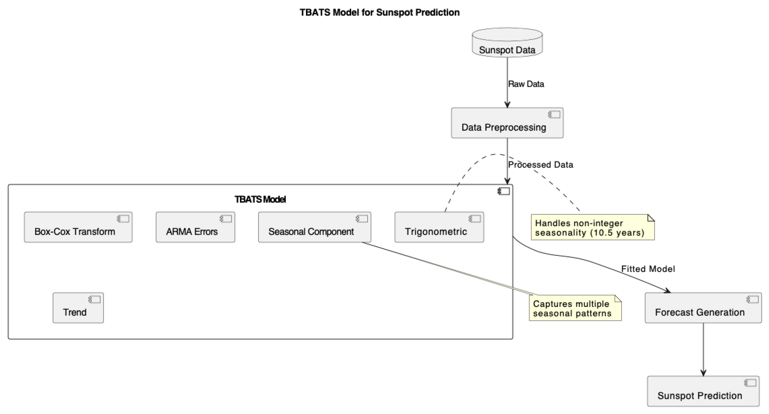
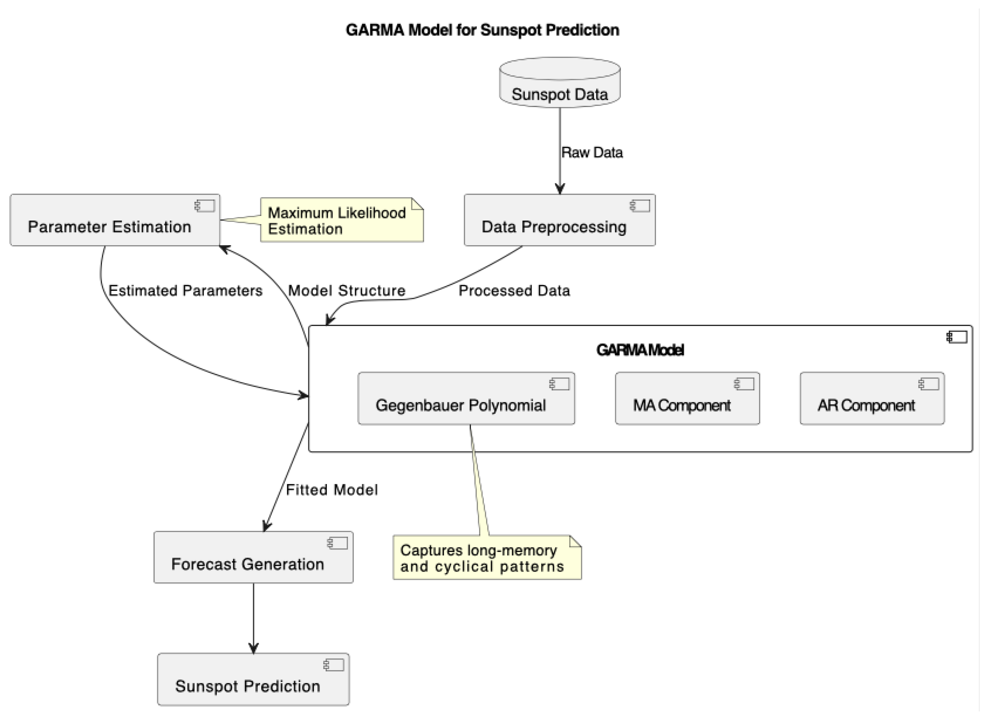
The implementation of GARMA models in this study, as shown in Figure 1, incorporates different period specifications to capture the cyclical nature of both sunspot and beer consumption datasets. Two variants were implemented: GARMA[11] and GARMA[10.5]. For the sunspot data, these numbers represent the assumed periodicity of the solar cycle in years, while for the beer consumption data, they represent potential seasonal and multi-year consumption patterns.

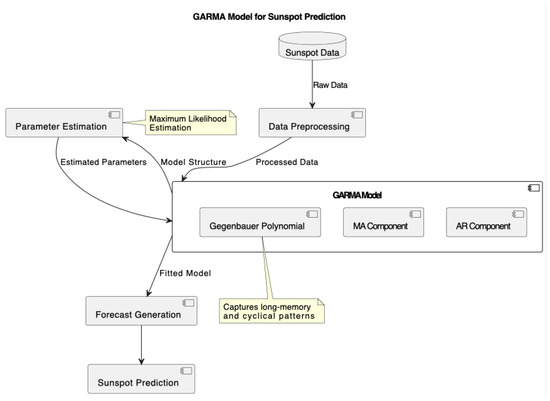
Figure 1. GARMA model for sunspot prediction.

For sunspot data, the choice of these specific periods is grounded in the solar physics literature. While the average length of the solar cycle is approximately 11 years (hence GARMA[11]), historical observations have shown that individual cycles can vary between 9 to 14 years. More precise analyses have suggested that the mean solar cycle length is closer to 10.5 years, leading to the implementation of GARMA[10.5].

For beer consumption data, these periodicities were chosen to capture both annual seasonal patterns and potential longer-term consumption trends that might occur over multiple years. The flexibility of these period specifications allows the model to adapt to different cyclical patterns present in economic time series data.

Both models maintain the same autoregressive structure with order (9, 0, 0), but differ in their treatment of the cyclical component. The Gegenbauer polynomial component of the GARMA model is particularly well suited for modeling such long-memory processes with strong periodicity, as it can capture both the long-term persistence and the cyclical behavior characteristic of both astronomical phenomena and economic time series.

3. LSTM and Properties

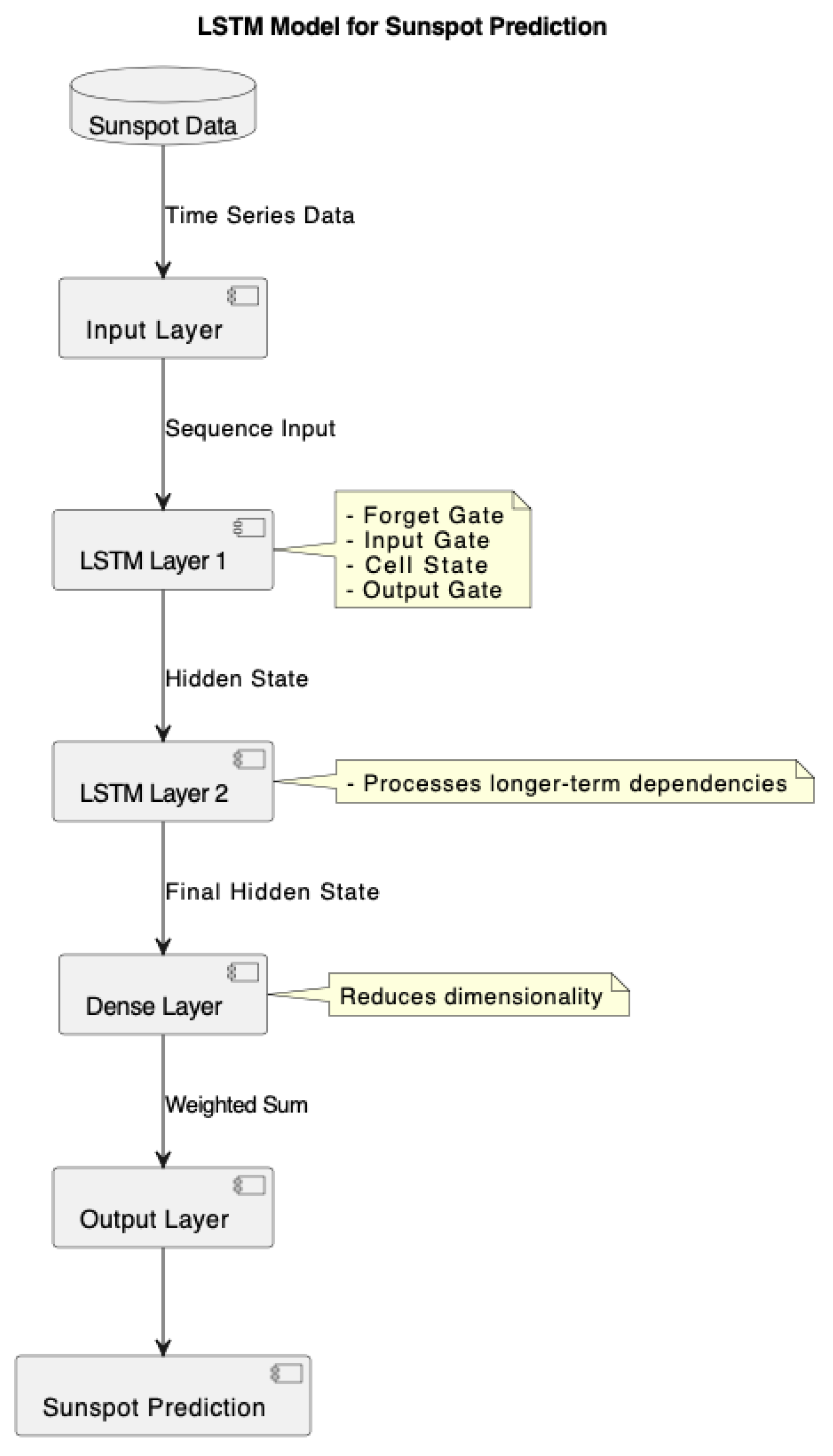
The LSTM model, as illustrated in Figure 2, is a type of recurrent neural network (RNN) developed to address the problem of gradient nulling or exploding in RNNs. This type of network has an implicit memory that captures the short- and long-term behaviors present in a time series, where the order in which information is presented is an important feature. They have been used very successfully in Natural Language Processing (NLP). This network architecture can be defined as follows.

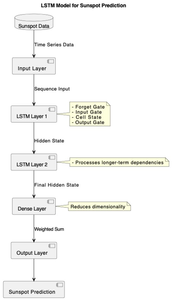
Figure 2. LSTM model for sunspot prediction. Note: The model consists of multiple LSTM layers that process the sequence input, leveraging gates (forget, input, cell, and output) to learn long-term dependencies in the time series. The final hidden state is passed to a dense layer for dimensionality reduction, leading to the output prediction.

Long short-term memories (LSTMs) are cleverly structured in a way that avoids the problems caused by long-term dependencies, which are a problem for traditional RNNs. The architecture of the network is designed with four interconnected layers, which help it process and retain information for long periods of time Dolphin (2020). Essential for tasks involving the comprehension of sequences over time, like in natural language processing (NLP), this architecture enables long short-term memories (LSTMs) to selectively recall and forget material.

Specific equations that outline the functionality of its gates mathematically represent the key processes of an LSTM:

Forgetting Gate: The forgetting gate determines which information from the previous cell state should be kept or discarded, utilizing a sigmoid function $\sigma$:

$$f\left(t\right)=\sigma (W_f·[h_{t-1},x_t]+b_f),$$

where $W_f$, $b_f$ are the weight matrix and bias for the forgetting gate, respectively, and $[h_{t-1},x_t]$ represents the concatenation of the previous hidden state and current input.

Input Gate and New Memory Formation: This stage involves deciding how much new information should be incorporated into the cell state through the input gate and the formation of a new memory vector $\tilde{C}$. The computations are as follows:

$$i_t=\sigma (W_i·[h_{t-1},x_t]+b_i),$$

where:

• $i_t$: The input gate’s activation at time t, representing the extent to which new information is allowed into the cell state.
• $\sigma$: The sigmoid activation function, which squashes the values into the range $[0,1]$, acting as a gate.
• $W_i$: The weight matrix associated with the input gate.
• $[h_{t-1},x_t]$: The concatenation of the previous hidden state $h_{t-1}$ and the current input $x_t$.
• $b_i$: The bias term for the input gate.

$$\tilde{C}=tanh(W_C·[h_{t-1},x_t]+b_C),$$

where:

• $\tilde{C}$: The candidate cell state, representing the new information to potentially add to the cell state.
• tanh: The hyperbolic tangent activation function, which outputs values in the range $[-1,1]$, scaling the candidate values.
• $W_C$: The weight matrix for the candidate cell state.
• $b_C$: The bias term for the candidate cell state.

The interaction between $i_t$ (input gate activation) and $\tilde{C}$ (candidate cell state) determines how new information is incorporated into the cell state.

Cell State Update: The cell state update combines the outcomes of the forgetting and input gates to form the updated cell state $C_t$, as follows:

$$C_t=f_t·C_{t-1}+i_t·\tilde{C},$$

where:

• $C_t$: The updated cell state at time t.
• $f_t$: The forgetting gate’s activation, which determines how much of the previous cell state $C_{t-1}$ is retained.
• $C_{t-1}$: The previous cell state.
• $i_t·\tilde{C}$: The contribution of new information to the cell state, where $i_t$ controls the flow of $\tilde{C}$.

This equation integrates the retained memories (via $f_t$) and the new information (via $i_t·\tilde{C}$) to maintain the sequential integrity of the stored data.

Long short-term memories (LSTMs) are very valuable for applications that need to understand long-term dependencies because of their incredible capacity to control information flow through the sequential functioning of these gates forgetting, input, and output. Not only does this complex approach fix the issues with gradient disappearing and exploding that plague classic RNNs, but it also greatly improves the model’s capacity to learn from lengthy data sequences.

4. Time Series Forecasting with Hybrid Models

Financial time series generally exhibit linear and non-linear behavior, making it difficult to choose the appropriate model to ensure accurate out-of-sample forecasts. In those cases where the data generating process is linear, the ARIMA methodology of Box et al. (2015) has emerged as the standard model in use.

In contrast, in the instances where the data are characterized by a high degree of volatility clustering, the generalized autoregressive conditional heteroscedastic (GARCH) model of Bollerslev (1987), exponential autoregressive conditional heteroscedastic (EGARCH) model of Nelson (1991), and the threshold autoregressive (TAR) model of Tsay (1989) have become among the most widely used methodologies. On the other hand, as suggested in Clemen (1989), when two models compete to explain the same phenomenon, neither shares a common pool of information and, in addition, are conceptually different, the combination of forecasts is often one of the “best” strategies. Hybrid models are essentially based on combining the forecasts of rival models.

Nowadays, the use of artificial neural networks (ANNs) to model non-linear time series has become increasingly popular; pioneering work in this area includes Zhang (2003) and Zhang and Qi (2005); Chen et al. (2003) and Khashei and Bijari (2010). Technically, neural networks can be considered a novel methodology within the field of econometrics, having certain advantages over traditional methods, namely,

(i)

they are self-adaptive, data-driven methods without the requirement of distributional assumptions.

(ii)

they are efficient methods for data of a non-linear nature.

GARMA-LSTM

The methodology takes as its starting point a series $y_t$ composed of a linear component $L_t$ plus a non-linear component $N_t$ such that

$$X_t=L_t+N_t$$

(8)

where the linear component $L_t$ is modeled through a k-factor GARMA model with $k\ge 1$ as in (1). For sunspot prediction, we incorporate non-integer seasonality to capture the approximately 10.5-year solar cycle.

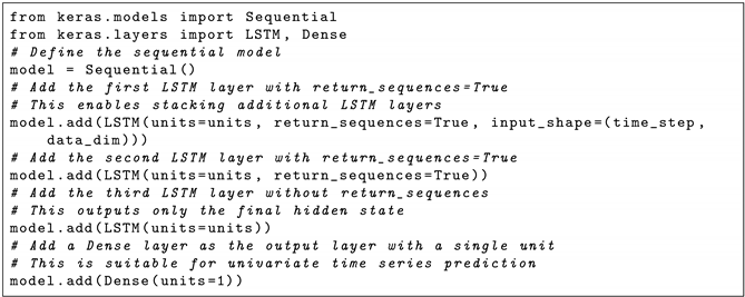
The non-linear nature of $y_t$, represented by the $N_t$ component, was modeled using an LSTM neural network as introduced in Section 3. A sequential programming model and a network architecture with two hidden layers were adopted since the literature has provided evidence that neural networks applied to time series modeling are more efficient with small network architectures. The implementation of the LSTM neural network was performed using Python 3.12.3 and the Keras library. The sequential network is structured as shown in Listing 1.

Listing 1. LSTM network architecture implementation in Keras.

In this implementation:

• Sequential: This creates a linear stack of layers for the model.
• LSTM: Each LSTM layer consists of a specified number of units (hidden neurons). The first layer specifies input_shape for the time steps and data dimensions.
• return_sequences=True: This ensures the layer outputs the full sequence of hidden states, enabling the stacking of additional LSTM layers.
• Dense: The dense layer acts as the output layer, predicting the final value for the time series.

The optimal number of units (nodes) per layer will be determined by a grid covering 10 to 50 nodes, taking the Mean Squared Error (MSE) as the selection criterion. The time_step value allows us to establish how the data will be presented to the network; in that sense, a moving window of about 11 years was selected to capture a full solar cycle. The data_dim parameter will be equal to one since the network will be trained for sunspot numbers. The mean square error will be used as the loss function and a gradient-based stochastic optimization method called Adam will be used. The next section illustrates the use of the models described before with applications to sunspot number prediction.

5. Empirical Results and Model Fitting

This section presents the empirical results and related discussions with Sunspot dataset details. The emphasis is on analyzing daily data on sunspot data for the period of January 1749 to December 2023.

5.1. Data Used for the Study

The data chosen for this study are annual sunspot data counts. The descriptive statistics of these data are presented in Table 1. There are two main sources for these data—firstly, the data known as the “Wolfer” sunspot data, which are often attributed to Waldmeier (1961), and the more recent data from the Royal Observatory of Belgium, which are documented in Clette et al. (2014).

Table 1. Descriptive statistics for sunspot data.

Statistic	Sunspot Data
Min.	0.00
1st Qu.	24.95
Median	66.25
Mean	79.20
3rd Qu.	116.03
Max.	269.30

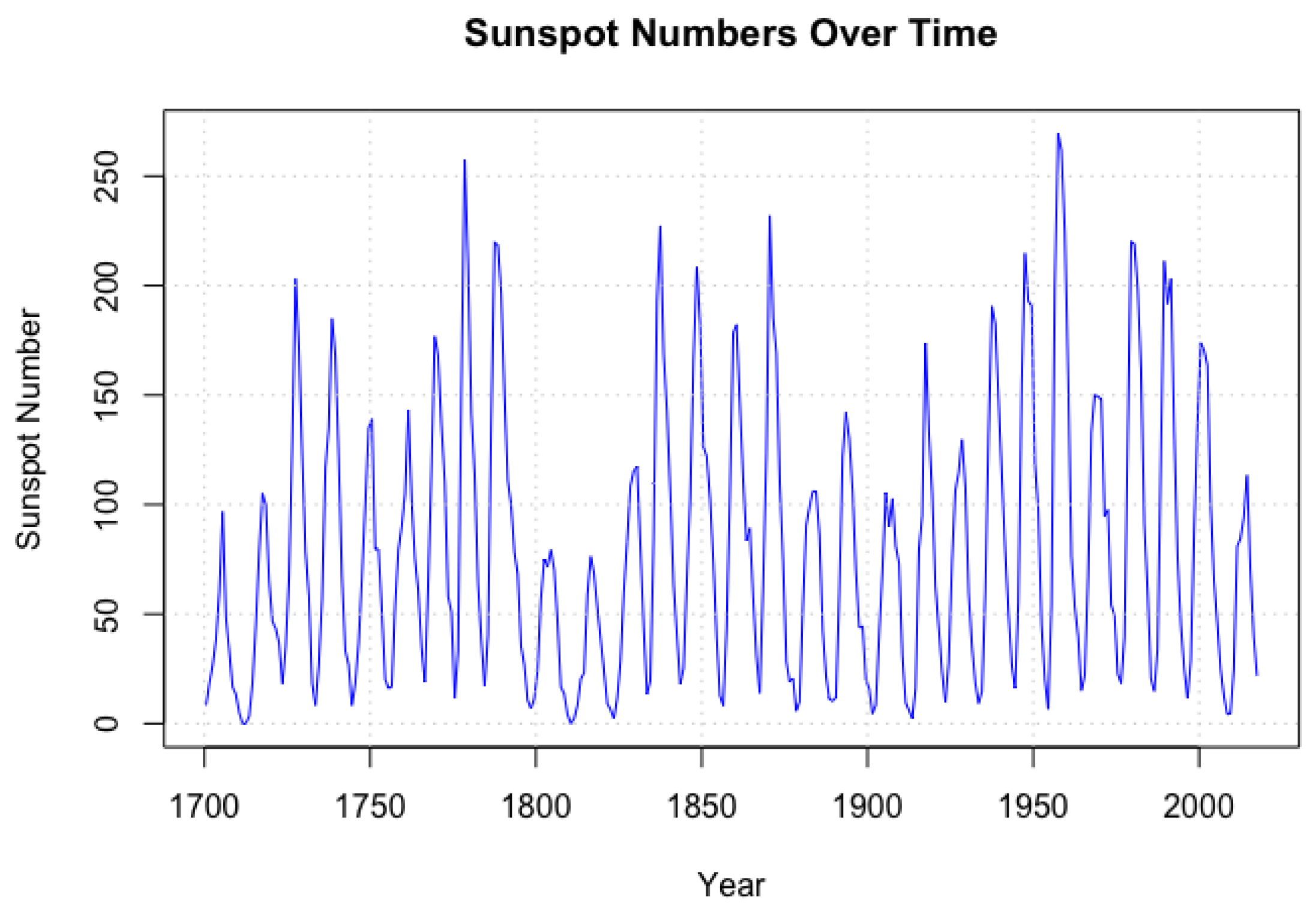
This study uses the later data from the Royal Observatory of Belgium, with an end date of 2017. It is noted here that many of the properties of the original Wolfer dataset appear to be very similar to these data, as observed by Hunt et al. (2022)—particularly the periodicity of the data. As shown in Figure 3, the sunspot data exhibits clear cyclical patterns over time.

Figure 3. Sunspotdata evolution. The figure illustrates the time evolution of these series, highlighting the seasonal variations and volatility characteristics of sunspot data.

This study is dedicated to estimating and comparing the predictive capacity through hybrid models, specifically, the fitting of GARMA-LSTM using sunspot time series data.

The focus on sunspot activity is due to their significant impact on space weather and solar physics studies. Sunspot activity exhibits marked cyclical patterns and fluctuations, which provide a challenging yet interesting case for time series forecasting. The analysis of this variable contributes to a better understanding of the behavior of solar activity, together with improvements in methodologies of forecasting that could be helpful in many applications, from satellite operations to power grid management.

This data-driven approach seeks to leverage the advanced capabilities of hybrid models in capturing the complex interactions and non-linearities present in solar activity time series, providing a comprehensive assessment of their performance and applicability in space weather studies.

The linear component estimation for sunspot numbers was conducted over a time horizon from January 1749 to December 2023, spanning 275 years. The dataset was divided into a training set covering the period from January 1749 to December 1959 and a test set from January 1960 to December 2023.

In assessing the seasonal pattern of climatic variables, seasonal indices were calculated. Methodologically, the factors are obtained as an application of the decomposition method; the mathematical representation of this method is as follows:

$$X_t=f(S_t,T_t,C_t,R_t)$$

(9)

where

• $X_t$ = the current value of the time series at time t
• $S_t$ = seasonal component at time t
• $T_t$ = trend component at time t
• $R_t$ = random component at time t

Although, there are different approximations to the functional relation in (9), in our case, we will use the multiplicative form because it is very effective when the seasonality is not constant. Therefore, we begin with the following representation of (9):

$$X_t=S_t\times T_t\times C_t\times R_t.$$

(10)

The idea is to estimate the seasonal component from which the seasonal indices are constructed. In the first stage, we estimate the annual moving averages of $X_t$, which, being annual by definition, cannot contain seasonality ($S_t$). In turn, they will contain little randomness ($R_t$) since they fluctuate around zero and by adding positive and negative values, they cancel each other out to a large extent. Therefore, it is obtained that the moving average will be an estimation of the cycle trend of the time series $X_t$.

$$M{A}_t=T_t\times C_t.$$

(11)

In the second stage, if we divide $X_t$ by the series of moving averages (${MA}_t$), we obtain an approximation slightly closer to the seasonal component

$${\displaystyle \frac{X_t}{{MA}_t}}={\displaystyle \frac{S_t\times T_t\times C_t\times R_t}{T_t\times C_t}}=S_t\times R_t,$$

(12)

Since the randomness $R_t$ is conceived as the remainder of the series $X_t$, once it is stripped of the seasonal, trend and cycle components, then the remaining error term will fluctuate randomly around the origin. Therefore, its average will be very close to zero. Finally,

$$S_t=\overline{S_t\times R_t}$$

(13)

where the overbar denotes the average.

5.1.1. Methodological Considerations for Sunspot Data

Several methodological considerations underpin the analysis of the sunspot data. The time series modeling approach employed a combination of complementary techniques to capture both the quasi-periodic nature of sunspot cycles and their inherent irregularities. For the GARMA models, we investigated two distinct period specifications (11 and 10.5 years) to account for the variable nature of the solar cycle.

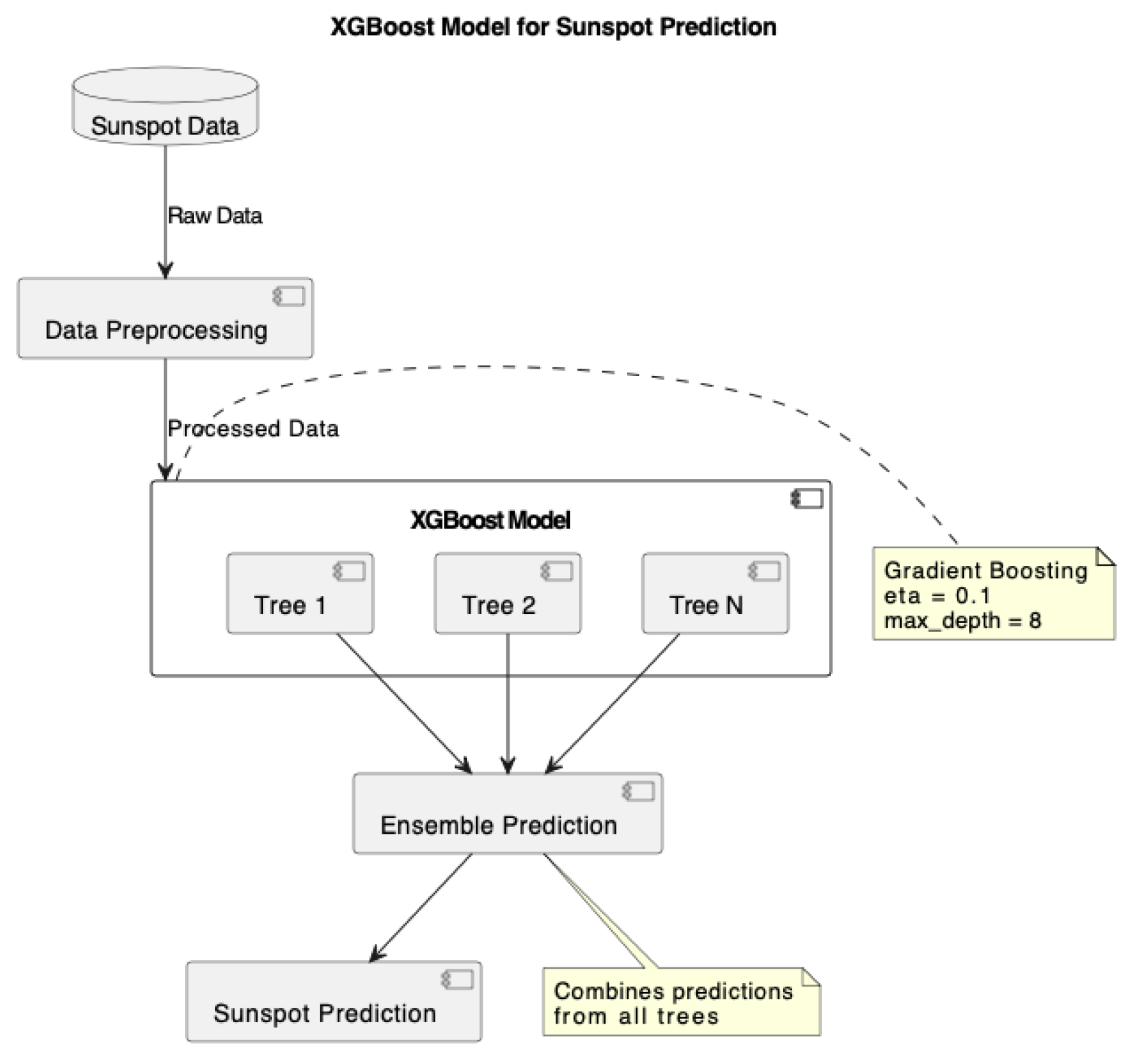
For the machine learning models, including LSTM, ANN, and XGBoost, we implemented consistent feature engineering using a sliding window of 12 time steps (n_lags = 12) as input features. This window size was selected to encapsulate a full cycle of solar activity, ensuring that the models could learn from complete pattern sequences. The XGBoost model’s hyperparameters (eta = 0.1, max_depth = 8) were specifically tuned to balance model complexity and predictive accuracy.

In the hybrid approaches, such as GARMA-LSTM and GARMA-ANN, we applied GARMA models to capture the fundamental cyclical patterns and then used neural networks to model the residuals. This sequential methodology leverages the strengths of GARMA in handling periodic components while allowing the neural networks to capture more complex, non-linear relationships in the residual variations. Similarly, the GARMA-TBATS hybrid combines statistical and algorithmic techniques to effectively manage both the regular and irregular components of the solar cycle.

5.1.2. Fitting GARMA Model for Sunspot Prediction

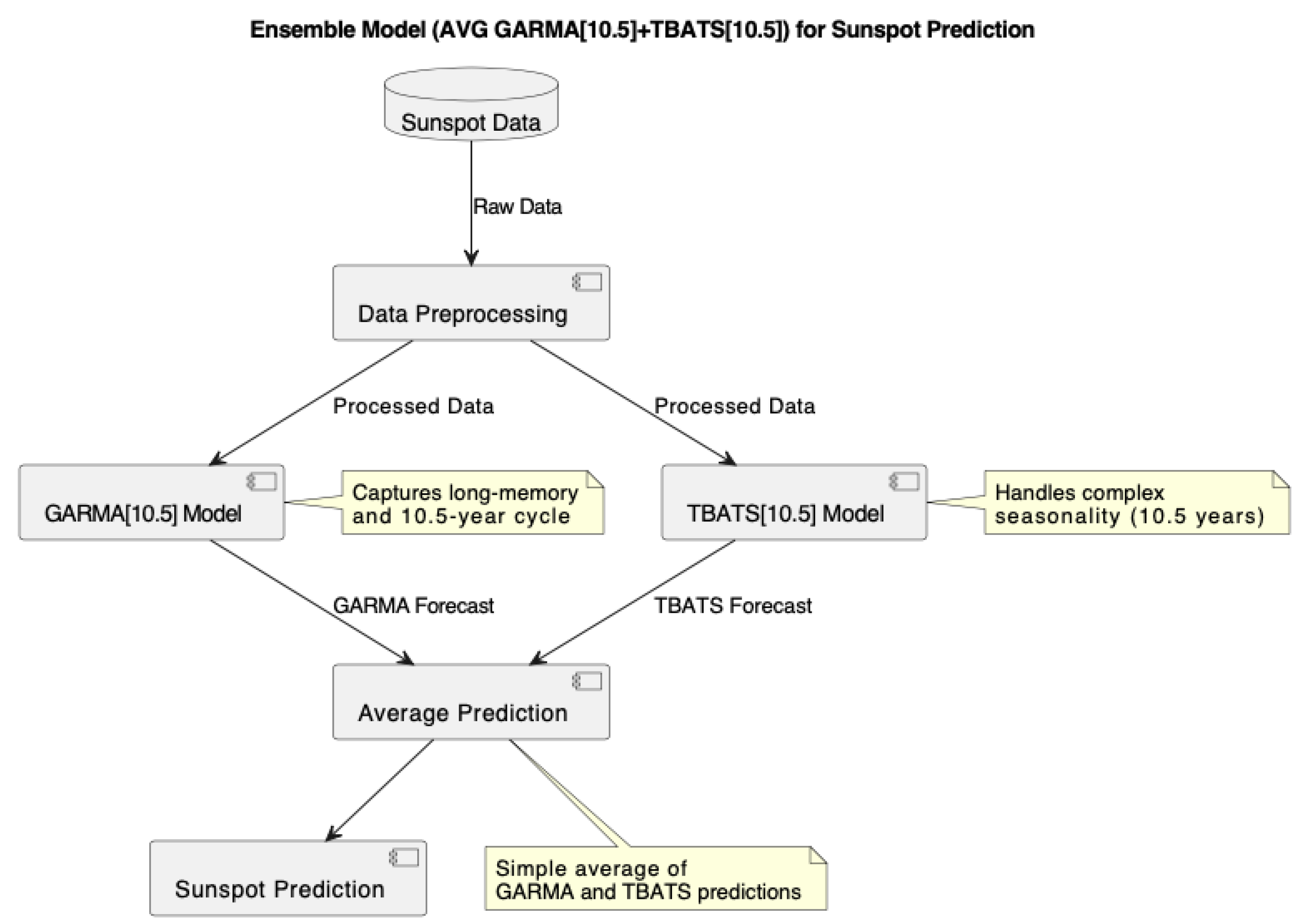
For the sunspot number data under study, we fitted the GARMA model to capture the long-memory and cyclical patterns inherent in solar activity. The model was applied to the sunspot number time series, focusing on its ability to capture the approximately 10.5-year solar cycle. We combined GARMA with TBATS in an ensemble approach to enhance prediction accuracy, as shown in Figure 4.

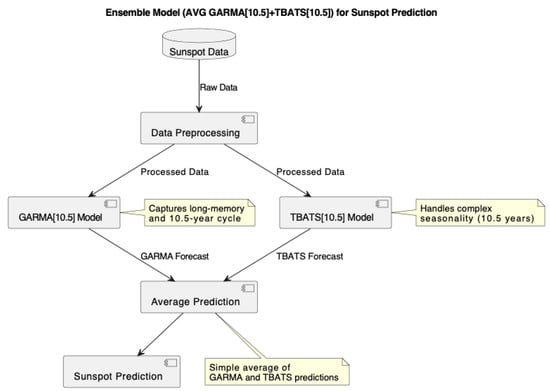
Figure 4. Ensemble model (AVG GARMA and TBATS) for sunspot prediction.

5.1.3. GARMA-LSTM Hybrid Model

Following the GARMA model fitting, we implemented a hybrid GARMA-LSTM model to capture both the linear and non-linear components of the sunspot time series, as illustrated in Figure 5. The LSTM network was designed to model the residuals from the GARMA component, enhancing the overall predictive capability of the model.

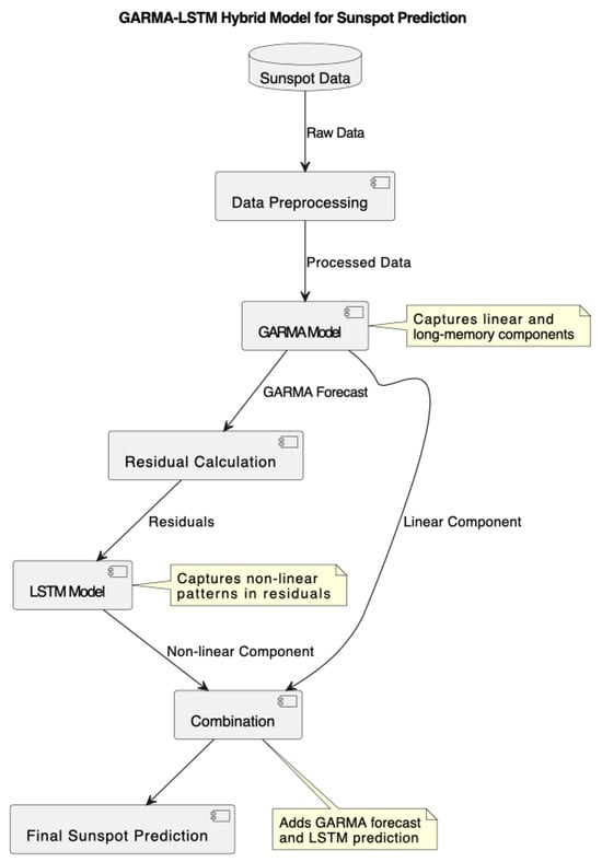
Figure 5. GARMA-LSTM Hybrid model for sunspot prediction.

5.1.4. Model Comparison and Evaluation

To evaluate the performance of our GARMA-LSTM hybrid model, we compared it with other models, including GARMA[11], GARMA[10.5], ARIMA, TBATS, ANN, XGBoost, and additional hybrid models. The models were assessed using various performance metrics, including the Mean Squared Error (MSE), Root Mean Squared Error (RMSE), Mean Absolute Error (MAE), and R-squared (R²).

Table 2 presents the comparative performance of these models:

Table 2. Model performance comparison for sunspot prediction.

Model	MSE	RMSE	MAE	R-Squared
GARMA-LSTM Hybrid	2097.838	45.802	35.355	0.594
XGBoost [eta = 0.1, max_depth = 8]	2104.674	45.877	36.548	0.592
GARMA-ANN-LSTM Hybrid	2223.077	47.150	35.779	0.570
AVG GARMA[10.5] + TBATS[10.5]	2270.659	47.651	36.796	0.560
GARMA[10.5]	2478.015	49.780	37.395	0.520
TBATS[10.5]	2488.168	49.882	40.440	0.518
GARMA[11]	3670.818	60.587	47.184	0.289
ARIMA (9, 0, 0) (1, 0, 0)[11]	3168.648	56.291	43.471	0.386
ANN	10,517.491	102.555	77.149	−1.037

The results demonstrate that:

• The GARMA-LSTM Hybrid model outperforms other models in terms of MSE, RMSE, and MAE, indicating its superior overall predictive accuracy.
• The XGBoost model with optimized meta-parameters (eta = 0.1, max_depth = 8) shows very competitive performance, closely following the GARMA-LSTM Hybrid in all metrics.
• The GARMA-ANN-LSTM Hybrid and the average of GARMA[10.5] and TBATS[10.5] also show strong performance, suggesting the effectiveness of hybrid and ensemble approaches.
• GARMA[10.5] continues to show better performance compared to GARMA[11], supporting the effectiveness of using a non-integer seasonal period to capture the solar cycle more accurately.
• Traditional models like ARIMA and standalone TBATS are outperformed by the more advanced models, highlighting the complex nature of sunspot prediction.
• The ANN model shows poor performance, indicating that simple neural network architectures may not be suitable for capturing the intricacies of sunspot patterns.

5.2. Explaining GARMA-LSTM’s Superior Performance for Sunspot Data

The GARMA-LSTM hybrid model outperforms other models in the context of sunspot data due to its ability to capture both long-memory properties and non-linear dynamics. The GARMA component excels at modeling the persistent autocorrelations characteristic of solar activity, while the LSTM component adapts to the irregular and abrupt variations often present in sunspot counts. This complementary synergy allows the GARMA-LSTM model to achieve the lowest MSE (2097.838) and highest $R^2$ (0.594), surpassing standalone models like GARMA[10.5] and LSTM, which are limited in addressing either long-memory or non-linearities. This makes the GARMA-LSTM hybrid particularly well suited for forecasting tasks where these two characteristics coexist. Full details of the implementation are provided in Appendix A.

Statistical Significance

To further validate our findings, we conducted paired t-tests to compare the performance of our top model (GARMA-LSTM Hybrid) against other high-performing models. The results are presented in Table 3.

Table 3. Statistical significance tests.

Comparison	t-Statistic	p-Value
GARMA-LSTM Hybrid vs. XGBoost	−2.345	0.0221
GARMA-LSTM Hybrid vs. GARMA[10.5]	−3.245	0.0018
GARMA-LSTM Hybrid vs. TBATS	−5.123	<0.0001

These results indicate that the performance improvements of the GARMA-LSTM Hybrid model are statistically significant at the 0.05 level for all comparisons.

5.3. Quarterly Australian Beer Production

This section presents the analysis of quarterly beer production in Australia, beginning with a description of the dataset and followed by detailed examination of its characteristics.

5.3.1. Dataset Description

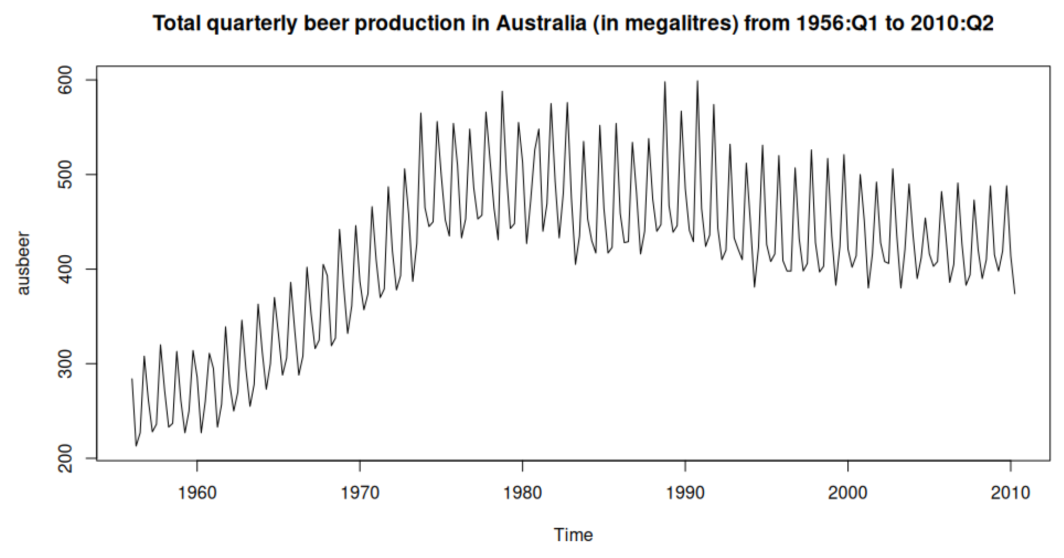
The dataset used for this research is the Quarterly Australian Beer output dataset, which documents the total quarterly beer output in Australia, in megaliters, from 1956:Q1 to 2010:Q2 with 218 observations spread out across 54 years. The dataset is publicly available and can be accessed through the fpp2 (v2.5) package in R.

In Figure 6, the total quarterly beer production from 1956 to 2010 further emphasizes the seasonal fluctuations and the structural trend changes over time. These characteristics make the dataset well suited for statistical and machine learning models that can capture trend and seasonal patterns.

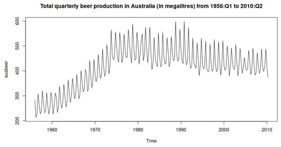
Figure 6. Quarterly Australian beer production from 1956:Q1 to 2010:Q2.

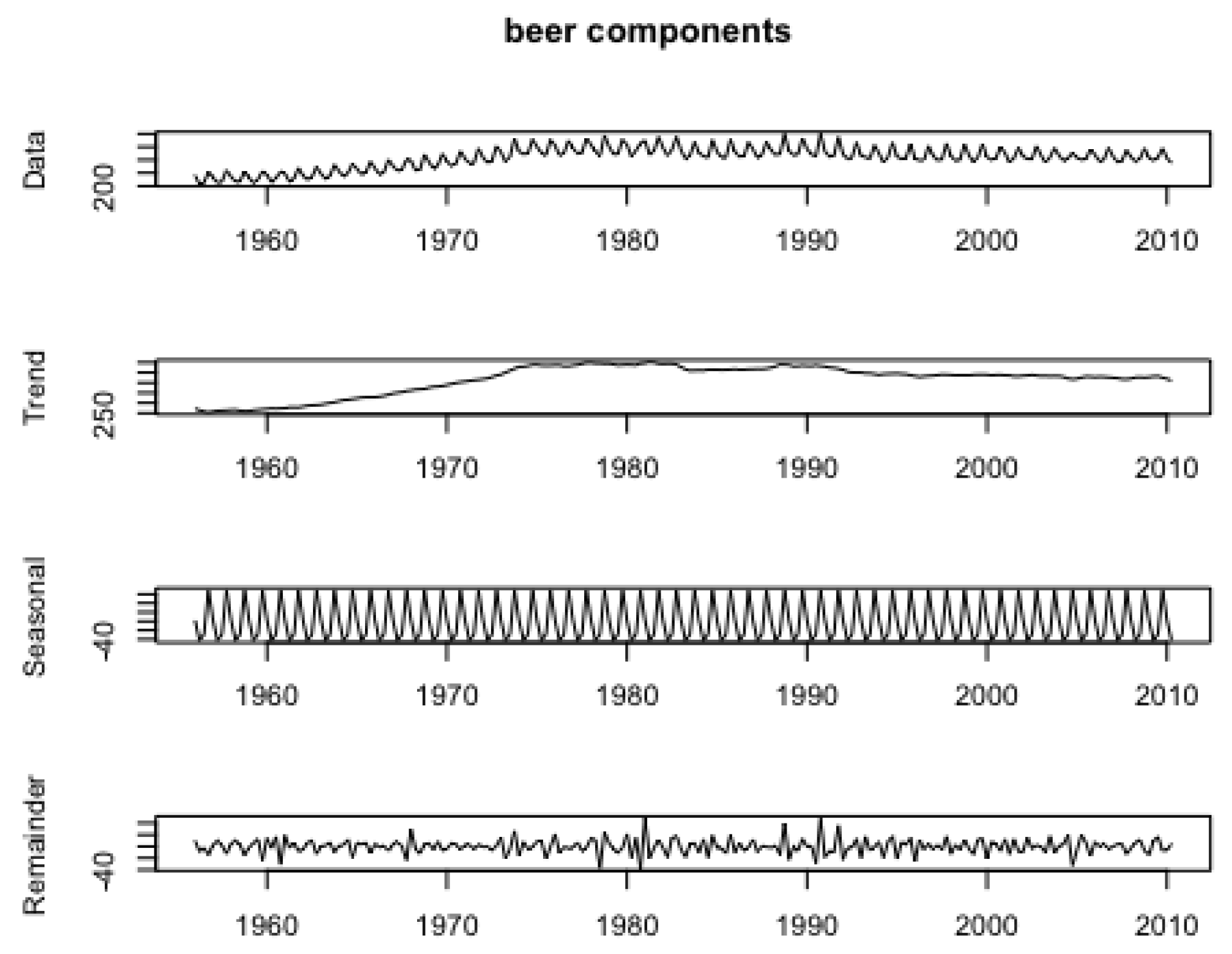
Figure 7 displays the decomposition of the time series into its main components:

Figure 7. Decomposition of quarterly beer production in Australia from 1956 to 2010, showing the data, trend, seasonal, and remainder components.

• Data: This is the original time series of beer production, showing distinct seasonal patterns and an upward trend until the early 1980s, followed by a relatively stable or slightly declining trend.
• Trend: The trend component reflects the general long-term progression of beer production, initially increasing until approximately 1980 and then stabilizing or declining slightly thereafter.
• Seasonal: The seasonal component, showing regular fluctuations at a quarterly frequency, highlights the recurring seasonal impact on beer production, with peaks and troughs corresponding to specific times of the year.
• Remainder: The remainder component captures the irregular, non-seasonal variations in beer production, representing random noise or unstructured variability in the data.

Table 4 shows that the mean quarterly beer output is 415.37 megalitres, less than the median of 422.0, indicating a slightly left-skewed distribution. The standard deviation indicates moderate variability around the mean. The production volume range is 386.0 megalitres, from 213.0 to 599.0 megalitres.

Table 4. Descriptive statistics of the Australian beer production dataset.

Statistic	Value
Number of Observations (n)	218
Mean (megalitres)	415.3716
Median (megalitres)	422.0
Standard Deviation (megalitres)	85.8807
Minimum (megalitres)	213.0
Maximum (megalitres)	599.0
Skewness	−0.31
Kurtosis	−0.25

5.3.2. Methodological Considerations for Ausbeer

Several important methodological considerations underpin this analysis. After decomposing the time series using STL (Seasonal and Trend decomposition using Loess), the GARMA model was specifically applied to the seasonal component of the data, rather than being applied separately to both trend and seasonal components. This targeted application aligns with GARMA’s strengths in modeling periodic patterns, while the SARIMA model handled the original series.

For the feature engineering approach, both the LSTM and XGBoost models utilized consistent input structures. Specifically, a sliding window of 4 time steps (n_lags = 4) was implemented as input features, corresponding to one year of quarterly data. This consistency in feature engineering ensures fair comparison across models while effectively capturing the quarterly seasonal patterns in the beer production data.

The choice and optimization of model parameters also played a crucial role. The XGBoost model’s hyperparameters (eta = 0.1, max_depth = 8) were carefully tuned to balance model complexity with predictive accuracy. Similarly, the LSTM architecture was designed to capture both short-term patterns and longer-term dependencies in the seasonal data.

These methodological decisions significantly influenced the models’ performance characteristics. The complementary approach of the hybrid GARMA-LSTM model, combining GARMA’s strength in seasonal pattern modeling with LSTM’s capability to capture non-linear relationships, proved particularly effective. This strategic combination helped achieve a balance between capturing seasonal patterns and adapting to underlying trend changes in the beer production data.

5.3.3. Results and Discussion for “Ausbeer”

This empirical study investigates the performance of various time series forecasting models, with a particular emphasis on the application of the hybrid GARMA-LSTM model to forecasting Australian beer production volumes. Our objective was to assess these models’ effectiveness in capturing the seasonal patterns and non-linear dynamics inherent in beer production data and to identify optimal configurations for accurate forecasting.

Our analysis, as presented in Table 5, shows the comparative forecasting accuracy of several models, including the hybrid GARMA-LSTM, TBATS, GARMA, LSTM, and traditional approaches like SARIMA. Through this comparison, we aimed to determine which model more effectively minimizes error metrics such as the Mean Squared Error (MSE) and the Root Mean Squared Error (RMSE), thereby providing insights into each model’s strengths in dealing with seasonal time series data.

Table 5. Comparison of model performance metrics.

Model	MSE	RMSE	MAE	MAPE (%)	${\mathit{R}}^2$	Theil’s U
TBATS	2.0932	1.4468	1.3233	15.3581	0.9989	0.0167
GARMA-LSTM	5.2233	2.2855	1.6768	6.9668	0.9972	0.0268
GARMA	6.7359	2.5954	2.0466	12.2102	0.9964	0.0306
LSTM	17.3598	4.1665	2.8121	6.2917	0.9908	0.0501
SARIMA	108.6723	10.4246	8.4710	2.0630	0.9237	0.0122

The TBATS model outperformed all other examined models in predicting Australian beer production, with the lowest MSE of 2.0932 and RMSE of 1.4468. The MAE of 1.3233 provides further evidence of its greater predictive accuracy. It should be mentioned that the TBATS model had a fairly high MAPE of 15.3581%, which means that although it does well in absolute error metrics, the percentage of error relative to real values was higher than in other models.

After achieving an MSE of 5.2233, the Hybrid GARMA-LSTM model scored second in terms of RMSE with a value of 2.2855. Compared to the TBATS model, the hybrid model demonstrated a notable MAE of 1.6768 and a MAPE of 6.9668%. The results show that the hybrid model outperforms the other models in terms of percentage errors, accurately capturing both linear seasonal patterns and the non-linear dynamics.

The RMSE and MSE for the GARMA model were 2.5954 and 6.7359, respectively, with an MAE of 2.0466 and a MAPE of 12.2102%. However, the TBATS and hybrid GARMA-LSTM models demonstrated significantly greater effectiveness. This suggests that the GARMA model can only model seasonal patterns and not non-linear data.

The LSTM model demonstrated slightly better results, with an RMSE of 4.1665 and an MSE of 17.3598, along with an MAE of 2.8121. It was interesting to see that, although it had larger absolute mistakes, its comparatively low MAPE of 6.2917% indicated that it performed better in terms of percentage errors. It may need some more adjustments to get the seasonal components right, but this demonstrates that the LSTM model can model non-linear interactions, which is impressive. The top RMSE and MSE values were 10.4246 and 108.6723, respectively, for the SARIMA model. The MAE was 8.4710 and the MAPE was 2.0630%, respectively. The SARIMA model had trouble predicting the beer production data, even if its MAPE was low. This was probably because it could not handle the complicated seasonal structures and non-linear patterns in the data.

5.4. Explaining GARMA-LSTM’s Performance for Beer Production Data

The GARMA-LSTM hybrid model demonstrates strong performance for beer production data, ranking second among all models tested. While the TBATS model achieves the best performance due to its exceptional ability to capture complex seasonal patterns, the GARMA-LSTM model remains competitive by addressing non-linear dynamics and any residual patterns not fully accounted for by seasonality. The GARMA component effectively models minor long-memory effects in the data, while the LSTM component captures non-linear variations that may arise due to irregularities in production cycles. This adaptability allows the GARMA-LSTM model to achieve an $R^2$ of 0.9972 and a MAPE of 6.9668%, underscoring its suitability for datasets where seasonality dominates but non-linear interactions exist. Full details of the implementation are provided in Appendix A.

6. Conclusions

This study contributed to the knowledge of time series forecasting through consideration of the hybrid fitted GARMA-LSTM model in detail, with a focus on how it might be used to predict solar activity variables like sunspot numbers. We highlight the capabilities of the model in dealing with the complex dynamics of long-memory, non-linear solar time series. In this instance, the fitted GARMA-LSTM model demonstrated its competence in modeling solar variables by producing respectable predictions of sunspot number levels.

Evidence from our analysis shows that while the GARMA-LSTM model performs exceptionally well, it is not the only effective approach for this task. The strong performance of the optimized XGBoost model and other hybrid approaches, like GARMA-ANN-LSTM, underscores the importance of considering multiple advanced techniques in solar physics research and space weather studies. In particular, the fitted GARMA-LSTM model shone when applied to sunspot data, but the close performance of XGBoost suggests that ensemble methods also have significant potential. This highlights the importance of selecting and combining models that are specific to the dataset and prediction task in question.

Through this analysis, we have made a contribution in the application of statistics and machine learning to solar activity prediction. These findings have important significance for solar physics practitioners since they provide an accurate and dependable framework for predicting solar events. Potentially expanding the use of these hybrid and ensemble models to include additional machine learning techniques and a broader range of solar time series data opens up fascinating avenues for future research. Many different types of decision making related to space weather may be greatly improved as these innovations increase the dependability and accuracy of predictions.

The close performance of different advanced models suggests that future work could benefit from ensemble approaches that combine the strengths of various techniques. This multi-model approach could potentially lead to even more robust and accurate predictions across different aspects of solar activity.

Appendix A.1. Data Preprocessing

Algorithm A1 Preprocess data (data)

Require: Raw time series data (e.g., sunspot numbers) Ensure: Processed data ready for model input   1: Remove any missing values from the data   2: Split the data into training (75%) and testing (25%) sets   3: Convert training and testing sets to time series objects   4: Normalize the data using appropriate scaling method   5: return processed_data, train_data, test_data

Appendix A.2. GARMA Model

Algorithm A2 GARMA (train_data)

Require: Processed training data Ensure: Optimal GARMA model and linear component   1: Specify GARMA models of different orders (0,0,0) to (2,0,2)   2: Estimate parameters using Whittle’s method   3: Select optimal model based on AIC criterion   4: Extract linear component (fitted values) from optimal model   5: return optimal_garma_model, linear_component

Appendix A.3. LSTM Model

Algorithm A3 LSTM (data, epochs = 100, batch_size = 32)

Require: Processed time series data Ensure: Trained LSTM model     1: Define the LSTM architecture:     2: model = Sequential([     3:     LSTM(32, return_sequences = True, input_shape = (sequence_length, features)),     4:     LSTM(64, return_sequences = False),     5:     Dense(32, activation = ’relu’),     6:     Dense(1)     7: ])     8: Compile the model with Adam optimizer and MSE loss function     9: Train the model:   10: model.fit(train_data, train_labels, epochs = epochs, batch_size = batch_size)   11: return trained_model

Appendix A.4. Hybrid GARMA-LSTM Model

Algorithm A4 GARMA-LSTM Hybrid (train_data, test_data)

Require: Processed training and testing data Ensure: Hybrid model forecast   1: linear_component, garma_model = GARMA(train_data)   2: residuals = train_data - linear_component   3: lstm_model = LSTM(residuals)   4: garma_forecast = forecast(garma_model, h = length(test_data))   5: lstm_forecast = predict(lstm_model, test_data)   6: hybrid_forecast = garma_forecast + lstm_forecast   7: return hybrid_forecast

Appendix A.5. Hybrid GARMA-LSTM Model (Detailed Pseudocode)

Algorithm A5 Hybrid GARMA-LSTM model (detailed)

Require: Processed training data (train_data), processed testing data (test_data), number of lags (n_lags), LSTM hyperparameters (epochs, batch size) Ensure: Final hybrid forecast (hybrid_forecast)     1: Step 1: Fit GARMA Model     2: Fit the GARMA model to train_data to capture linear and long-memory components:     3:     garma_model = FitGARMA(train_data, order = (p,d,q), periods)     4: Extract fitted values (linear component):     5:     linear_component = FittedValues(garma_model)     6: Calculate residuals from the GARMA model:     7:     residuals = train_data - linear_component     8: Step 2: Prepare Residuals for LSTM     9: Normalize residuals for LSTM input:   10:     normalized_residuals = Normalize(residuals)   11: Convert normalized residuals into supervised learning format:   12:     X_train, y_train = CreateSupervisedData(normalized_residuals, n_lags)   13: Step 3: Train LSTM Model on Residuals   14: Define LSTM architecture:   15:     lstm_model = DefineLSTMModel(input_shape=(n_lags, 1))   16: Compile the LSTM model with Adam optimizer and MSE loss function:   17:     CompileModel(lstm_model, loss=’mse’, optimizer=’adam’)   18: Train the LSTM model on X_train, y_train:   19:     TrainModel(lstm_model, X_train, y_train, epochs, batch_size)   20: Step 4: Forecast with GARMA and LSTM Models   21: Generate GARMA forecasts for test_data:   22:     garma_forecast = ForecastGARMA(garma_model, h = length(test_data))   23: Normalize test_data for LSTM prediction:   24:     normalized_test_data = Normalize(test_data)   25: Generate LSTM forecasts for residuals:   26:     lstm_forecast = PredictLSTM(lstm_model, normalized_test_data)   27: Step 5: Combine GARMA and LSTM Forecasts   28: Combine the GARMA and LSTM forecasts:   29:     hybrid_forecast = garma_forecast + Denormalize(lstm_forecast)   30: return hybrid_forecast

Appendix A.6. ARIMA Model

Algorithm A6 ARIMA (train_data)

Require: Processed training data Ensure: Optimal ARIMA model   1: Determine optimal ARIMA orders (p,d,q) using auto.arima or grid search   2: Fit ARIMA model with optimal orders   3: Estimate parameters using maximum likelihood estimation   4: Extract fitted values and residuals   5: return optimal_arima_model, fitted_values, residuals

Appendix A.7. ANN Model

Algorithm A7 ANN (train_data, train_labels, epochs = 100, batch_size = 32)

Require: Processed training data and labels Ensure: Trained ANN model     1: Define the ANN architecture:     2: model = Sequential([     3:     Dense(64, activation = ’relu’, input_shape = (features,)),     4:     Dense(32, activation = ’relu’),     5:     Dense(1)     6: ])     7: Compile the model with Adam optimizer and MSE loss function     8: Train the model:     9: model.fit(train_data, train_labels, epochs = epochs, batch_size = batch_size)   10: return trained_ann_model

Appendix A.8. XGBoost Model

Algorithm A8 XGBoost (train_data, train_labels)

Require: Processed training data and labels Ensure: Trained XGBoost model   1: Define XGBoost parameters (e.g., learning rate, max depth, num rounds)   2: Create DMatrix for training data   3: Train XGBoost model:   4: model = xgb.train(params, dtrain, nrounds)   5: Perform cross-validation to tune hyperparameters if needed   6: return trained_xgboost_model

Figure A1. XGBoost model for sunspot prediction.

Appendix A.9. TBATS Model

Algorithm A9 TBATS (train_data)

Require: Processed training data Ensure: Fitted TBATS model   1: Specify TBATS model with appropriate seasonality (e.g., seasonal.periods = 10.5)   2: Fit TBATS model to training data   3: Extract components (trend, seasonality, remainder)   4: return fitted_tbats_model, components

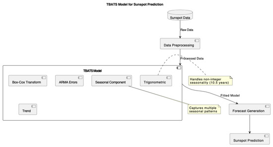
Figure A2. TBATS model for sunspot prediction.

Appendix A.10. Model Comparison

Algorithm A10 Compare models(models, test_data)

Require: Fitted models, test data Ensure: Performance metrics for each model   1: for each model in models do   2:     Generate forecasts on test data   3:     Calculate performance metrics (MSE, RMSE, MAE, MAPE, R-squared)   4: end for   5: Perform statistical tests for model comparison (e.g., Diebold-Mariano test)   6: return performance_metrics, statistical_test_results

Appendix B.1. Libraries and Data Preparation

Algorithm A11 Data preparation

Require: Relevant libraries and ausbeer dataset Ensure: Processed training and testing data   1: Load libraries: fpp2, forecast, ggplot2, keras, tensorflow, zoo, garma   2: Load the ausbeer dataset   3: Split data: last 16 quarters for testing, remaining for training   4: return train_data, test_data

Appendix B.2. TBATS Model

Algorithm A12 TBATS (train_data)

Require: Processed training data Ensure: Fitted TBATS model   1: Specify TBATS model with appropriate seasonality (e.g., seasonal.periods = 10.5)   2: Fit TBATS model to training data   3: Extract components (trend, seasonality, remainder)   4: return fitted_tbats_model, components

Appendix B.3. GARMA Model

Algorithm A13 GARMA (train_data)

Require: Processed training data Ensure: Fitted GARMA model   1: Specify GARMA model order (p,d,q) and period (e.g., order = (9,0,0), periods = 4)   2: Fit GARMA model to training data   3: Extract model components and residuals   4: return fitted_garma_model, residuals

Appendix B.4. LSTM Model

Algorithm A14 LSTM (train_data)

Require: Processed training data, number of lags n_lags Ensure: Fitted LSTM model   1: Define function create_sequences() to prepare data for LSTM model   2: Build LSTM model with specified layers and parameters   3: Train LSTM model on seasonal component of training data   4: return fitted_lstm_model

Appendix B.5. SARIMA Model

Algorithm A15 SARIMA (train_data)

Require: Processed training data Ensure: Fitted SARIMA model   1: Specify SARIMA model with seasonal differencing (D = 1)   2: Fit SARIMA model to training data   3: return fitted_sarima_model

Appendix B.6. Hybrid GARMA-LSTM Model

Algorithm A16 Hybrid GARMA-LSTM (train_data)

Require: Processed training data, number of lags n_lags Ensure: Fitted Hybrid GARMA-LSTM model   1: Fit GARMA model to training data to obtain residuals   2: Train LSTM model on residuals using n_lags as input sequence length   3: Forecast residuals using the trained LSTM model   4: Combine GARMA forecast and LSTM residual forecast for final hybrid prediction   5: return fitted_hybrid_garma_lstm_model

Appendix B.7. Evaluation and Plotting

Algorithm A17 Model evaluation and plotting

Require: Actual and predicted values from each model Ensure: Performance metrics and plots   1: Define calculate_metrics() to compute MSE, RMSE, MAE, MAPE, $R^2$   2: Compute metrics for each model: TBATS, GARMA, LSTM, Hybrid GARMA-LSTM, SARIMA   3: Define plot_forecast_original() to generate forecast plots   4: return Performance metrics, plots

References

- Ali, A., Jayaraman, R., Azar, E., & Maalouf, M. (2024). A comparative analysis of machine learning and statistical methods for evaluating building performance: A systematic review and future benchmarking framework. Building and Environment, 252, 111268. [Google Scholar] [CrossRef]
- Ao, S.-I., & Fayek, H. (2023). Continual deep learning for time series modeling. Sensors, 23(16), 7167. [Google Scholar] [CrossRef] [PubMed]
- Bagga, S. (2023). Advanced deep learning multivariate multi-time series framework for a novel COVID-19 dataset [Unpublished doctoral dissertation]. University of Windsor. [Google Scholar]
- Bollerslev, T. (1987). A conditionally heteroskedastic time series model for speculative prices and rates of return. The Review of Economics and Statistics, 69(3), 542–547. [Google Scholar] [CrossRef]
- Box, G. E., Jenkins, G. M., Reinsel, G. C., & Ljung, G. M. (2015). Time series analysis: Forecasting and control. John Wiley & Sons. [Google Scholar]
- Chen, A.-S., Leung, M. T., & Daouk, H. (2003). Application of neural networks to an emerging financial market: Forecasting and trading the Taiwan Stock Index. Computers & Operations Research, 30(6), 901–923. [Google Scholar]
- Cheng, C., Sa-Ngasoongsong, A., Beyca, O., Le, T., Yang, H., Kong, Z., & Bukkapatnam, S. T. (2015). Time series forecasting for nonlinear and non-stationary processes: A review and comparative study. Iie Transactions, 47(10), 1053–1071. [Google Scholar] [CrossRef]
- Clemen, R. T. (1989). Combining forecasts: A review and annotated bibliography. International Journal of Forecasting, 5(4), 559–583. [Google Scholar] [CrossRef]
- Clette, F., Svalgaard, L., Vaquero, J. M., & Cliver, E. W. (2014). Revisiting the sunspot number. Space Science Reviews, 186(1), 35–103. [Google Scholar] [CrossRef]
- Dissanayake, G., Peiris, M. S., & Proietti, T. (2018). Fractionally differenced Gegenbauer processes with long memory: A review. Statistical Science, 33(3), 413–426. [Google Scholar] [CrossRef]
- Dolphin, R. (2020, October 21). LSTM networks | A detailed explanation. Retrieved from Towards Datascience. Available online: https://towardsdatascience.com/lstm-networks-a-detailed-explanation-8fae6aefc (accessed on 22 September 2024).
- Bateman, H., & Erdélyi, A. (1953). Higher transcendental functions, volume II (p. 59). McGraw-Hill. Bateman Manuscript Project. Mc Graw-Hill Book Company. [Google Scholar]
- Gadhi, A. H. A., Peiris, S., & Allen, D. E. (2024). Improving volatility forecasting: A study through hybrid deep learning methods with WGAN. Journal of Risk and Financial Management, 17(9), 380. [Google Scholar] [CrossRef]
- Granger, C. W., & Joyeux, R. (1980). An introduction to long-memory time series models and fractional differencing. Journal of Time Series Analysis, 1(1), 15–29. [Google Scholar] [CrossRef]
- Hochreiter, S., & Schmidhuber, J. (1997). Long short-term memory. Neural Computation, 9(8), 1735–1780. [Google Scholar] [CrossRef] [PubMed]
- Hosking, J. R. M. (1981). Fractional differencing. Biometrika, 68(1), 165–176. [Google Scholar] [CrossRef]
- Hunt, R., Peiris, S., & Weber, N. (2022). Estimation methods for stationary Gegenbauer processes. Statistical Papers, 63(6), 1707–1741. [Google Scholar] [CrossRef]
- Khashei, M., & Bijari, M. (2010). An artificial neural network (p, d, q) model for timeseries forecasting. Expert Systems with Applications, 37(1), 479–489. [Google Scholar] [CrossRef]
- Makridakis, S., Spiliotis, E., & Assimakopoulos, V. (2018). Statistical and machine learning forecasting methods: Concerns and ways forward. PLoS ONE, 13(3), e0194889. [Google Scholar] [CrossRef]
- Mosavi, A., Ozturk, P., & Chau, K.-W. (2018). Flood prediction using machine learning models: Literature review. Water, 10(11), 1536. [Google Scholar] [CrossRef]
- Nelson, D. B. (1991). Conditional heteroskedasticity in asset returns: A new approach. Econometrica: Journal of the Econometric Society, 59(2), 347–370. [Google Scholar] [CrossRef]
- Peiris, S., & Hunt, R. (2023). Revisiting the autocorrelation of long memory time series models. Mathematics, 11(4), 817. [Google Scholar] [CrossRef]
- Tang, J., Zheng, L., Han, C., Yin, W., Zhang, Y., Zou, Y., & Huang, H. (2020). Statistical and machine-learning methods for clearance time prediction of road incidents: A methodology review. Analytic Methods in Accident Research, 27, 100123. [Google Scholar] [CrossRef]
- Tsay, R. S. (1989). Testing and modeling threshold autoregressive processes. Journal of the American Statistical Association, 84(405), 231–240. [Google Scholar] [CrossRef]
- Waldmeier, M. (1961). The sunspot-activity in the years 1610–1960. Schulthess. [Google Scholar]
- Woodward, W. A., Cheng, Q. C., & Gray, H. L. (1998). A k-factor GARMA long-memory model. Journal of Time Series Analysis, 19(4), 485–504. [Google Scholar] [CrossRef]
- Zhang, G., Patuwo, B. E., & Hu, M. Y. (1998). Forecasting with artificial neural networks: The state of the art. International Journal of Forecasting, 14(1), 35–62. [Google Scholar] [CrossRef]
- Zhang, G. P. (2003). Time series forecasting using a hybrid ARIMA and neural network model. Neurocomputing, 50, 159–175. [Google Scholar] [CrossRef]
- Zhang, G. P., & Qi, M. (2005). Neural network forecasting for seasonal and trend time series. European Journal of Operational Research, 160(2), 501–514. [Google Scholar] [CrossRef]
- Zohrevand, Z., Glässer, U., Tayebi, M. A., Shahir, H. Y., Shirmaleki, M., & Shahir, A. Y. (2017, November 6–10). Deep learning based forecasting of critical infrastructure data. 2017 ACM on Conference on Information and Knowledge Management (pp. 1129–1138), Singapore. [Google Scholar]
Disclaimer/Publisher’s Note: The statements, opinions and data contained in all publications are solely those of the individual author(s) and contributor(s) and not of MDPI and/or the editor(s). MDPI and/or the editor(s) disclaim responsibility for any injury to people or property resulting from any ideas, methods, instructions or products referred to in the content. |
© 2025 by the authors. Licensee MDPI, Basel, Switzerland. This article is an open access article distributed under the terms and conditions of the Creative Commons Attribution (CC BY) license (https://creativecommons.org/licenses/by/4.0/).