Hierarchical Semantic Correspondence Analysis on Feature Classes between Two Geospatial Datasets Using a Graph Embedding Method

Abstract

A method to find corresponding feature class pairs, including hierarchical M:N pairs between two geospatial datasets is proposed. Applying an overlapping analysis to the object sets within the feature classes, the similarities of the feature classes are estimated and projected onto a lower-dimensional vector space after applying the graph embedding method. In this space, conventional mathematical tools—agglomerative hierarchical clustering in this study—could be used to analyze semantic correspondences between the datasets and identify their hierarchical M:N corresponding pairs. The proposed method was applied to two cadastral parcel datasets; one for latest land-use records in an urban information system, and the other, for original land-use categories in the Korea land information system. To quantitatively assess identified feature pairs, F-measures for each pair are presented. The results showed that it was possible to find various semantic correspondences of the feature classes and infer regional land development characteristics.

1. Introduction

Establishing data integration between different geospatial information systems is necessary in order to set up geospatial data infrastructures for collecting and disseminating the data from different systems [1]. As each dataset belonging to these systems represents similar real-world entities or phenomena according to their own abstraction models and surveying rules, syntactic, structural, semantic, and geometric heterogeneities occur between corresponding objects of different datasets [2]. Among the mentioned heterogeneities, the first two can be addressed by applying well-known knowledge representation techniques, such as the web ontology language (OWL) or resource description framework (RDF), while remaining semantic; geometric ones, however, are still complicated problems [3]. This is due to the fact that corresponding spatial objects of different datasets, which represent the same real-world entity, have their own conceptual meanings and geometric representations according to the application purposes of datasets. For example, a small narrow road connecting a main road and a parking lot in a large commercial center may be represented as a polyline object attributed as “road” in one dataset, whereas it may be represented as a polygon object attributed as “auxiliary facility” in another dataset.

In the field of the map conflation, various methods have been developed to address the aforementioned semantic and geometric heterogeneity problems [4,5]. Authors in [5] proposed a conceptual framework for a general process to address these problems, as shown in Figure 1. In this process, a pre-processing step is performed to transform two geospatial datasets (GeoDSs) to have a uniform format, scale, reference system, and so on. Then, a semantic filter step is applied to identify the corresponding feature class pairs, which represent the same geographic entities or phenomena. While these two steps are related to model- (or dataset)-oriented analysis, the remaining steps correspond to the object-oriented analysis used to identify matching object pairs, and then, to address the geometric discrepancies between them.

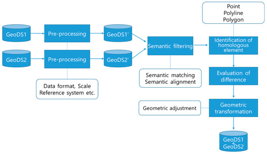
Figure 1. Conceptual framework of a general process to integrate two geospatial databases (adapted from [5]).

When the geospatial datasets to be integrated originate from a similar domain, a simple comparison of feature class names would provide the desired results for the semantic filter step. However, in the case when they are from different domains, the names can be the same or similar, even though the feature classes represent substantially different real-world entities or phenomena. Moreover, the corresponding relations may vary from 1:1 to 1:N or M:N. In these cases, detailed data specifications of the datasets to be compared are necessary. However, most of the datasets do not provide such information [6].

To address this problem, various object-based analysis techniques have been proposed. These techniques use matching objects between two datasets to identify corresponding feature classes. They assume that, if spatial objects of a certain feature class in one geospatial dataset correspond to spatial objects in another feature class in the other dataset with a high probability, there is high semantic similarity between the two feature classes [7]. Uitermark et al. [2] extended this method by introducing taxonomical and partonomical relationships of feature classes within each dataset, so that relations of feature classes between datasets, as well as within each dataset, can be obtained. Similarly, authors in [8,9] have proposed an ontology integration method based on searching for relations between objects, which are able to infer taxonomic relations between the feature classes. Cruz and Sunna [10] applied a graph-matching method, where a graph is constructed for each geospatial dataset, and the taxonomic and partonomical relations of feature classes of one geospatial dataset are represented as nodes and edges, respectively. This graph model has been adopted in some studies that proposed their own similarity measurement methods. Khatami et al. [3] combined several similarities for feature class name pairs and derived the overall object correspondence between feature classes (consequently, between geospatial datasets), as well as the semantic structure among feature classes (within a geospatial dataset). Buccella et al. [11] propose a novel system that manually creates domain ontologies and automatically enriches domain ontologies with standard information using semantic, syntactic, and structure analyses. Then, ontology integration is carried out with the information. Bhattacharjee and Ghosh [12] proposed the semantic hierarchy-based similarity measurement for semantic similarity between land cover feature classes, which considers a hop number from the top feature class node to a certain node in their graph. Kuo and Hong [13] proposed a conceptual framework for semantic integration of geospatial datasets, which allows identifying matching geospatial feature classes. In this framework, hierarchical semantic relations between the datasets such as “is_subset_of”, “is_superset_of”, or “is_same_to” were determined by analyzing intersection relations of objects belonging to feature classes. Kuai et al. [14] focused on natural language barriers for semantic matching between feature classes in different geospatial datasets. Recently, Zhang et al. [15] proposed a multi-feature-based similarity measurement based on geospatial relationships, feature catalog, and name tag, and then applied a supervised machine learning process to identify corresponding pairs.

Although the above studies showed good results, there is room for improvement by applying recent semantic analysis techniques [16,17,18] and developing new approaches to obtain hierarchical corresponding relations of feature classes between geospatial datasets, as well as within each dataset. These techniques begin from a co-occurrence matrix in which rows and columns represent individual entities used for analysis; in this study, feature classes are these entities. Considering the aforementioned object-based methods [7,8,9,10,11,12,13,14,15], these co-occurrence values could be measured by degrees of object sharing or intersection between feature classes from two geospatial datasets. This matrix representation easily shows overall degrees between feature classes—conventional mathematical tools—which are suitable for feature vector data but not matrix data and cannot be easily applied to the matrix for identifying corresponding feature class pairs. To address this problem, several dimensionality reduction techniques, such as latent semantic analysis or graph embedding, are employed to define a new vector space where individual entities are represented as feature vectors to which conventional mathematical tools can be easily applied [17,19,20].

In this study, the Laplacian graph embedding proposed in [20] was applied to address the above issue. This method was developed to identify the multi-level corresponding object–set pairs between two remote sensing data. It constructed a bipartite graph representing each object as a node, and node pairs’ similarities between datasets as an edge with a weighted value. Thereafter, by applying Laplacian graph embedding, objects with higher similarity were distributed on closer coordinates in the embedding space. Finally, a clustering analysis on the projected nodes in the space was conducted, and the hierarchical corresponding object–set pairs could be found. In this study, nodes are used to represent feature classes rather than individual objects, so that the feature class pairs between datasets with a greater number of shared objects have close coordinates in the embedding space. Thus, this space can be understood as a semantic feature space, where two feature classes representing similar real-world entities or phenomena have geometrically close embedding coordinates. Therefore, with the knowledge of these coordinates and their distances, which are proportional to semantic dissimilarity, the previously mentioned complicated correspondence relationship between the feature classes of the two geospatial datasets can be found, and the semantic relationships of the feature classes can also be compared and inferred.

In this paper, the proposed method is applied to cadastral parcels’ latest land-use records obtained from the urban information system (UIS) and their original land-use categories obtained from the Korea land information system (KLIS). These two systems have the same parcel dataset, however, attributes of their parcels could be different; a land-use category is assigned in the perspective of taxation, whereas the land-use record is assigned in the perspective of urban management. Consequently, even for the same parcels, their categories and records can be different, so that corresponding relations between these feature classes cannot be properly derived without having background information. These relations include not only M:N corresponding relations, but also their nested hierarchies. Moreover, these relations can be distinctive for specific areas due to unique geographical conditions typical for areas in question. The proposed method defines a semantic feature space where feature classes (in this study, the land-use category or land-use record) are represented as vectors. As conventional mathematical tools can be easily applied to vectors, and the distance between vectors in this study is proportional to semantic dissimilarity, the complicated relationships could be identified using proper mathematical tools such as clustering analysis.

The rest of the paper is organized as follows. In the subsequent section, an explanation of Laplacian graph embedding is given; in Section 3, the proposed method is explained; and in Section 4, it is applied for two areas, Seoul city to represent an urban area, and the Jeonnam Province to represent a rural area; then, their results are compared. Finally, in Section 5, the conclusions of this study are discussed.

2. Laplacian Graph Embedding

2.1. One-dimensional Embedding

In this paper, we assume an undirected and connected graph. The graph $G=\left(V,E\right)$ is represented by sets of vertices $V=\left\{v_i|i=1,\cdots ,N\right\}$ and edges $E=\left\{\left(v_i,v_j\right)|v_i,v_j\in V\right\}$. Given a weighted graph, edge weights are represented as a weight matrix $W\in R^{N\times N}$. One-dimensional graph embedding finds a configuration of embedded vertices in one-dimensional space, such that the vertices’ proximities from the edge weights are preserved as the embedded vertices’ distances. Assuming each entry of a column vector $x={\left(x(1),\cdots ,x(n)\right)}^T$ as coordinates of the embedded vertices, this problem can be solved through minimization of the following objective function [21].

$${\displaystyle \sum _{(i,j)\in E}{\left(x(i)-x(j)\right)}^2 w_{i,j}}$$

(1)

This function could be minimized when vertices i and j with large $w_{i,j}$ are embedded at close coordinates, whereas vertices with small $w_{i,j}$ are embedded into distant coordinates. In this study, this mathematical property is applied as follows: feature classes (e.g., land-use category and record) with a greater degree of object sharing have close coordinates in their embedding space and feature classes with a lesser degree of object sharing have distant coordinates. Equation (1) can be expressed in a matrix operation form with a Laplacian matrix $L$, and can be represented as Equation (2) [19,20,21].

$$\frac{1}{2}{\displaystyle \sum _{(i,j)\in E}{\left(x(i)-x(j)\right)}^2 w_{i,j}}=x^T L x$$

(2)

where, the Laplacian matrix $L$ is defined as Equation (3) with a vertex degree matrix $D$ whose diagonal entries are obtained as $d_{i,i}={\displaystyle {\sum }_{j\ne i}w{ }_{i,j}}$ and the remaining entries are 0.

$$L=D-W$$

(3)

Now, the problem can be changed to find a vector $x$ that minimizes $x^{T}Lx$, and can be represented as Equation (4).

$$x=\arg \min x^{T}Lx$$

(4)

Since the value of $x^{T}Lx$ is vulnerable to the scaling of a vector $x$, a constraint $x^T B x=1$ is imposed to remove any such arbitrary scaling effect [17]. The diagonal matrix $B$ provides weights on the vertices, so that the higher $b_{i,i}$ is, the more important is that vertex [21]. Equation (4) with the constraint can be solved by the Lagrange multiplier method as in Equations (5)–(7).

$$F(x)=⟨Lx, x⟩-\lambda \left(⟨Bx,x⟩-1\right)$$

(5)

$$\frac{\partial F(x)}{\partial x}=x^T\left(L+L^T\right)-\lambda x^T\left(B+B^T\right)$$

(6)

$$2{\left(Lx\right)}^T=2\lambda {\left(Bx\right)}^T\Rightarrow Lx=\lambda Bx$$

(7)

Thus, the solution of one-dimensional embedding, $x$, is obtained by solving the eigenproblem $Lx=\lambda Bx$. However, according to the rank of matrix $L$, there could be more than one eigenvector. In the field of graph spectral theory, the eigenvector corresponding to the smallest eigenvalue larger than 0 is the proven solution, which is called a Fiedler vector. Thus, the coordinates of vertices in one-dimensional embedding are obtained as components of the Fiedler vector as represented by Equation (7).

2.2. k-dimensional Embedding

Now, consider k-dimensional graph embedding. These embedded coordinates are represented as an $n\times k$ matrix $X=\left[x_1,\cdots ,x_k\right]$, so that the ith row of $X$, $x(i )=\left(x_1(i),\cdots ,x_k(i)\right)$, contains the k-dimensional coordinates of vertex $v_i$. Now, an objective function is defined as Equation (8) with the constraint, $X^T B X=I$.

$$\frac{1}{2}{\displaystyle \sum _{i,j}{\Vert x(i )-x(j ) \Vert }^{ 2} w_{i,j}}=trace \left(X^{T}LX\right)$$

(8)

Sameh and Wisniewski [22] proved that the solution to this trace minimization problem is obtained by the k-eigenvectors of $LX=\lambda BX$ that correspond to its smallest eigenvalues other than 0. Thus, the solution of Equation (8) is obtained by a matrix $X=\left[x_1,\cdots ,x_k\right]$, where $x_i$ represents an eigenvector corresponding to eigenvalue ${\lambda }_i$ under the condition $0={\lambda }_{ 0}<\lambda { }_1\le \cdots \le {\lambda }_k$.

However, the constraint $X^T B X=I$ normalizes the scales of the coordinates in each dimension. Thus, it is necessary to rescale them according to each dimension’s relative importance. Sameh and Wisniewski also proved that the minimum value of $X^{T}L X$ in Equation (8) equals the sum of the corresponding eigenvalues, as shown by Equation (9) [22].

$$\min trace \left(X^{T}L X\right)={\displaystyle \sum _{i=1}^k{\lambda }_i}$$

(9)

Accordingly, we can assume the eigenvalue ${\lambda }_i$ as the amount of either the penalty or the cost caused by the ith dimensional space in the embedding problem. So, when $k<l$, it is appropriate to apply more weight to $\left|x_k(i)-x_l(j)\right|$ than $\left|x_k(i)-x_l(j)\right|$ in measuring the proximity for a clustering analysis. Based on these mathematical properties, we determined the embedded coordinates as Equation (10), because the increase in distance is proportional to that of the root-squared coordinate difference [20].

$$X=\left[\frac{x_1}{\sqrt{{\lambda }_1}},\cdots ,\frac{x_k}{\sqrt{{\lambda }_k}}\right]$$

(10)

3. Proposed Method

The proposed method begins with an edge weight matrix whose cells represent the degree of object sharing between two feature classes (Step 1). From this matrix, k-dimensional feature vectors for each feature class are obtained by the Laplacian graph embedding technique (Step 2). Then, agglomerative hierarchical co-clustering is applied to find hierarchically corresponding feature class–set pairs (Step 3). Figure 2 presents a pseudocode of the proposed method and details of each step are explained in the following sections.

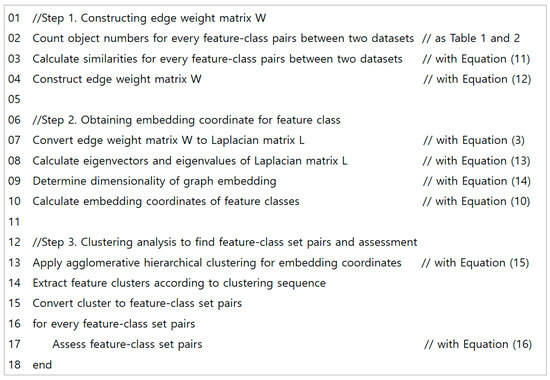
Figure 2. Pseudocode of the proposed method in this study.

3.1. Step 1: Constructing Edge Weight Matrix W

The proposed method begins with a weighted bipartite graph represented by a similarity matrix $S\in R^{n\times m}$, where $n$ and $m$ stand for the numbers of feature classes in two datasets $A$ and $B$ respectively, and cell values are calculated by Equation (11).

$$s(i,j)=\frac{N( f_i\cap f_j)}{\min (N(f_i),N(f_j))}$$

(11)

where, $N( )$ is a function that returns the number of spatial objects, $f_i$ and $f_j$ represents feature class i and j in two datasets $A$ and $B$, respectively. This similarity measure effectively explains a partial and complete relationship of two feature classes, which is necessary to find complicated corresponding pairs such as N:1, 1:M, or N:M [23,24].

Since Laplacian graph embedding assumes a normal graph, an edge weight matrix $W\in R^{N\times N}$, where $N=n+m$, is obtained by Equation (12). With this matrix $W$, its Laplacian matrix $L$ is obtained by Equation (3).

$$W=\left[\begin{array}{cc}0& S\\ S^T& 0\end{array}\right]$$

(12)

3.2. Step 2: Solving Eigenproblem and Obtaining K-dimensional Coordinates

The process of Laplacian graph embedding in Section 2 considered each vertices’ weight using a diagonal matrix $B$. However, in this study, each feature class has the same importance so that $B$ is set to an identity matrix and Equation (13) is applied instead of Equation (7).

$$L x=\lambda x$$

(13)

Although all the eigenvectors of Equation (13) are orthogonal and convey distinct information, we need to determine the optimal dimensionality k, because eigenvectors corresponding to small eigenvalues are appropriate for the embedding problem, as shown in Equation (9). The optimal dimensionality k for an expected number of clusters was proposed by [25]. Assuming each eigenvector has information to partition vertices into at least two clusters, he determined k as $\lceil {\log }_2 c\rceil$, where c is the expected number of clusters. ⌈ ⌉ is a function to present the minimum integer larger than a given value. Similarly, we determine k with Equation (14), because the maximum number of corresponding feature class pairs could not exceed the numbers of feature classes in either of two datasets.

$$k=\lceil {\log }_2 \left(\min \left(n,m\right)\right)\rceil$$

(14)

Accordingly, the embedded coordinates of the vertices in datasets $A$ and $B$ are obtained by k-rescaled eigenvectors corresponding to the k smallest eigenvalues other than 0, as in Equation (10).

3.3. Step 3: Agglomerative Hierarchical Clustering Analysis and Assessment of Clusters

Given clusters (at the initial condition, each feature class are considered as clusters), the agglomerative hierarchical clustering method searches the two closest clusters and merges them into one cluster. These searching and merging steps are repeated until all entities are merged into a single cluster. Thus, it presents a sequence of nested partitions of hierarchical cluster structure in the form of a dendrogram [26]. To apply the method, it is necessary to determine the criteria to measure the distance between two clusters. Among the several criteria, a single-link measure which considers the average distance of all entity pairs between clusters, as given in Equation (15), is chosen. The single-link measure defines the dissimilarity as the minimum distance among all the entity distances between two entity clusters and tends to find elongated clusters.

$$D\left(C_a, C_b\right)=\underset{i\in C_a j\in C_b}{\min }d\left(e_i, e_j\right)$$

(15)

where, $D \left(C_a,C_b\right)$ is a cluster distance of cluster $C_a, C_b$, $d\left(e_i, e_j\right)$ is an entity distance between embedded coordinates of feature class $f_i, f_j$. A dendrogram is a tree diagram that shows a structure of clusters where the bottom row of nodes represents individual entities (in this study, feature classes of two datasets) and the remaining nodes represent the merging of their sub-nodes. Thus, by analyzing the feature types in the remaining nodes, semantically corresponding feature classes between two datasets could be obtained.

The clustering analysis in the above step presents a clustering sequence, but not obtained are clusters from which semantically corresponding feature class–set pairs are determined. Thus, statistical assessment of these clusters is necessary. Given an lth cluster, $C^{\left(l\right)}$ needs to be divided into two feature class–sets, $C_a^{ \left(l\right)} \mathrm{and} C_b^{ \left(l\right)}$, according to the datasets to which the feature classes belong. Then, a criterion could be applied to assess the pairs $C_a^{ \left(l\right)} \mathrm{and} C_b^{ \left(l\right)}$ with the F-measure of Equation (16), which is often used in the field of semantic engineering and information retrieval [27]. F-measures of each and every cluster are calculated, and then the clusters whose F-measure is higher than a threshold are determined as semantically corresponding feature class–set pairs.

$$F-measure=\frac{2\times P_a^{ \left(l\right)}\times P_b^{ \left(l\right)}}{P_a^{ \left(l\right)}+P_b^{ \left(l\right)}}$$

(16)

where, $P_a^{\left(l\right)} \mathrm{and} P_b^{ \left(l\right)} \mathrm{are} \mathrm{obtained} \mathrm{by} \frac{{{\displaystyle \sum }}_{i\in C_a^{\left(l\right)}, j\in C_b^{\left(l\right)} }N\left(f_i{\displaystyle \cap }{f}_j\right)}{{{\displaystyle \sum }}_{i\in C_a^{\left(l\right)} }N\left(f_i\right)} \mathrm{and}$ $\frac{{{\displaystyle \sum }}_{i\in C_a^{\left(l\right)}, j\in C_b^{\left(l\right)} }N\left(f_i{\displaystyle \cap }{f}_j\right)}{{{\displaystyle \sum }}_{j\in C_b^{\left(l\right)} }N\left(f_j\right)}$, respectively.

4. Experiment and Results

4.1. Experimental Dataset

To evaluate the proposed method, two representative areas have been chosen, Seoul city and the Jeonnam Province, as shown in Figure 3, as the first one is the most urbanized area in the country, and the other is the Southwestern part of the country, which is well-known for fertile farmlands with vast plains. Land parcel datasets of the two areas were extracted from UIS and KLIS. Thereafter, each parcel’s land-use record and category were compared as shown in Table 1 and Table 2. In these tables, 1 to 21 refer to the record index, and A to T refer to the category index. The values of cells in the tables represent the number of land parcels having a certain index pair with record and category. There are several pairs whose record and category index names are the same, such as (9, A) of a dry paddy field, (11, B) of a paddy field, (20, H) of a parking lot, (17, N) of a river, which seem to be 1:1 corresponding pairs. However, for the land parcels of “N (River)”, there are 1416 parcels with “17 (river)” and 1345 parcels with “Road (16)”, which means that in terms of the land-use category in KLIS, the land parcels with “N (river)” are currently used for hydrology or transportation purpose with similar proportions. In terms of the land-use record in UIS for “17 (river)”, the land parcels were mainly registered as “N (River)” (1416 parcels); however, significant number of parcels (756 parcels) were registered as O (Ditch). This demonstrated that the corresponding land-use record and category pairs can be unexpectedly expanded according to concatenated one-to-many corresponding relations; consequently, a new method is required to identify complicated M:N corresponding feature class pairs between geospatial datasets. This method also needs to be based on the data itself, not on the geographic background knowledge of the area under consideration. In Table 2, the above relations are not valid and show completely different relations. This means that a data-driven learning method such as the one proposed in the present paper is required to obtain distinctive results for each area, for example, such as Seoul city and the Jeonnam Province.

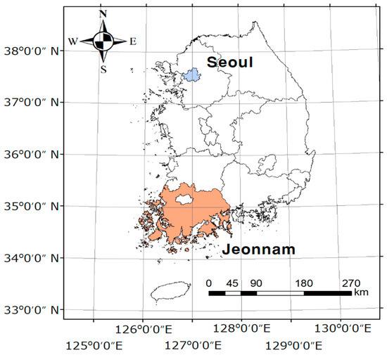
Figure 3. Experimental areas of Seoul city and the Jeonnam Province considered in this study.

Table 1. Comparison between land-use record in urban information system (UIS) and land-use category in the Korean land information system (KLIS) of about 800,000 land parcels in Seoul city.

	A	B	C	D	E	F	G	H	I	J	K	L	M	N	O	P	Q	R	S	T
1	1101	213	3	1329	364,662	6	25	17	3	2	955	272	24	85	126	0	16	11	57	307
2	85	18	0	57	11,364	0	1	1	0	1	45	6	0	0	2	0	0	0	0	23
3	101	28	0	112	69,118	0	1	0	0	2	130	5	2	1	18	0	12	0	2	36
4	215	45	0	382	20,065	9	16	1	1	0	629	29	2	28	30	1	0	9	11	51
5	309	139	0	180	97,089	106	5	35	843	2	313	148	7	32	38	8	7	9	9	281
6	71	47	0	25	11,852	29	8	4	14	1	120	12	1	8	26	0	1	1	5	144
7	145	66	1	57	79,864	12	6	4	2	0	278	31	2	18	25	2	3	0	6	86
8	158	118	1	17	3870	919	1	1	0	5	52	17	4	14	44	3	0	1	1	89
9	8392	5690	3	414	669	0	1	0	0	1	138	15	34	186	123	9	20	3	2	1167
10	224	22	80	128	4	0	0	0	0	0	1	0	0	0	5	1	0	0	0	2
11	62	3333	0	7	1	0	0	0	0	0	6	0	4	1	19	5	8	0	0	75
12	17	4	0	161	21	0	0	0	0	0	0	0	0	0	6	0	2	6	0	0
13	428	43	0	10,258	645	2	21	0	0	0	97	4	2	9	61	0	28	172	14	156
14	289	38	0	1254	395	1	10	0	0	0	24	1	0	8	16	1	1	50	1	208
15	26	6	0	415	35	0	8	0	0	0	5	0	1	2	14	0	9	9	17	22
16	2732	1865	1	2624	30,767	110	197	13	5	2	69,102	1460	346	1345	2977	80	301	291	45	1764
17	219	261	0	104	65	2	1	0	0	0	120	19	348	1416	756	59	6	4	0	97
18	119	79	0	247	1834	1	3	1	1	0	161	30	10	75	38	1	31	2200	8	109
19	120	89	0	29	114	5	1	0	0	0	44	12	2	14	7	1	1	15	0	14
20	46	104	0	36	381	1	0	387	2	0	45	2	3	6	30	5	0	7	0	52
21	61	10	0	36	144	0	5	0	1	0	19	16	3	157	12	3	3	1	0	166

1 (detached house), 2 (row house), 3 (multiplex house), 4 (apartment house), 5 (commercial building), 6 (business building), 7 (multipurpose building), 8 (industrial building), 9 (dry paddy field), 10 (orchard), 11 (paddy field), 12 (forestation field), 13 (natural forest field), 14 (grass field), 15 (bare soil field), 16 (road), 17 (river), 18 (park), 19 (gymnasium), 20 (parking lot), 21 (miscellaneous). A (Dry paddy field), B (Paddy field), C (Orchard), D (Forestry), E (Building site), F (Factory site), G (School site), H (Parking lot), I (Gas station site), J (Warehouse site), K (Road), L (Railway site), M (Bank), N (River), O (Ditch), P (Marsh), Q (Water supply site), R (Park). S (Gymnasium site), T (Miscellaneous).

Table 2. Comparison between land-use record in UIS and land-use category record in KLIS of about 4,000,000 land parcels in Jeonnam Province.

	A	B	C	D	E	F	G	H	I	J	K	L	M	N	O	P	Q	R	S	T
1	29,886	13,270	187	4603	537,129	25	218	9	6	92	350	112	6	73	55	110	6	1	238	3684
2	109	92	3	15	778	1	1	3	0	0	4	0	0	0	0	1	0	0	0	12
3	75	34	0	6	700	0	1	0	0	2	2	0	0	1	0	1	0	0	1	5
4	192	131	1	67	1289	3	4	0	0	0	17	0	0	0	15	1	0	0	0	13
5	1257	1567	15	269	33,248	88	14	38	936	85	114	27	0	2	9	10	2	0	7	2273
6	297	237	3	71	2978	4	46	12	4	30	2	24	0	2	2	0	1	0	10	242
7	1000	1148	11	148	27,633	15	9	11	51	32	24	22	0	4	8	19	1	0	19	976
8	875	688	7	257	1972	4634	0	2	14	125	40	0	7	9	7	22	1	7	0	1970
9	962,643	50,201	934	46,482	12,995	36	135	4	7	63	1038	401	17	448	115	623	57	13	116	4726
10	11,374	4357	7009	2382	337	1	8	3	0	13	15	2	2	5	2	21	1	0	6	161
11	27,823	1,170,616	338	4468	2736	23	43	3	0	48	1053	73	51	656	302	1613	50	4	34	7872
12	320	266	0	27,706	17	0	0	0	0	33	6	0	0	4		0	2	0	96	0
13	2442	1034	30	505,169	430	0	22	0	1	2	346	75	5	27	103	143	47	7	19	159
14	7919	4437	30	79,618	722	0	15	0	0	0	80	26	2	14	7	47	4	0	7	378
15	169	83	5	5155	64	2	9	1	0	19	11	37	1	0	2	21	77	9	98	255
16	14,357	20,976	47	8066	10,027	68	179	8	3	24	90,897	1605	121	916	774	459	751	8	39	1301
17	3182	8267	8	1752	450	5	11	0	0	2	343	20	1474	6083	9342	9110	97	1	2	792
18	169	140	0	109	194	0	0	1	0	0	6	4	0	4	3	10	0	240	3	69
19	114	201	0	83	311	0	212	0	0	0	23	29	0	2	4	1	5	7	0	0
20	124	151	1	45	231	1	9	214	5	0	20	2	0	0	3	2	2	0	2	152
21	885	889	5	313	713	2	123	0	1	7	19	18	17	5	5	221	18	0	20	1343

1 (detached house), 2 (row house), 3 (multiplex house), 4 (apartment house), 5 (commercial building), 6 (business building), 7 (multipurpose building), 8 (industrial building), 9 (dry paddy field), 10 (orchard), 11 (paddy field), 12 (forestation field), 13 (natural forest field), 14 (grass field), 15 (bare soil field), 16 (road), 17 (river), 18 (park), 19 (gymnasium), 20 (parking lot), 21 (miscellaneous). A (Dry paddy field), B (Paddy field), C (Orchard), D (Forestry), E (Building site), F (Factory site), G (School site), H (Parking lot), I (Gas station site), J (Warehouse site), K (Road), L (Railway site), M (Bank), N (River), O (Ditch), P (Marsh), Q (Water supply site), R (Park). S (Gymnasium site), T (Miscellaneous).

4.2. Results and Discussion

Figure 4 shows the projection of the data provided in Table 1 onto the three-dimensional space using the proposed method. Although the projection was originally done onto five-dimensional space, the coordinates of up to three principle dimensions are used for the visual analysis. As described above, the land-use record and category that are close to each other in this space share more land parcels, such as (11, B), as can be seen at the bottom left in the figure (this cell corresponds to a paddy field).

Figure 4. Projection of the land-use record and category of Table 1 onto a 3-dimensional space with the proposed method for visual presentation. Feature class pairs that share more objects, such as (11, B) and (20, H) in Table 1, have closer coordinates.

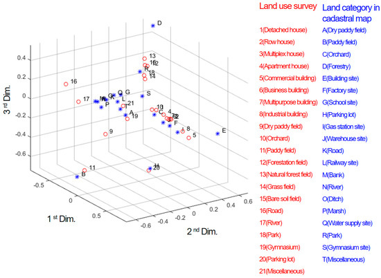
Figure 5 shows the dendrogram of agglomerative hierarchical clustering on the embedded coordinates of the data provided in Table 1. In the dendrogram, nodes and links represent the process used to identify the clusters. For example, “8 (industrial building)” and “J (Warehouse site)” first constitute a cluster C₁, to which “F (Factory site)” is clustered sequentially to transform the cluster into C₂₆. According to this clustering process, the corresponding land-use record and category pairs between UIS and KLIS were analyzed, and subsequently, the corresponding feature class clusters could be derived and analyzed accordingly. This clustering process allows the identification of not only 1:1 correspondences (at the right side of the dendrogram), but also complex correspondences. In addition, clusters such as C₁₈ and C₁₉ are combined to define a supercluster for higher-level geographic concepts for a so-called trans-hydro network. From the clustering results provided in Figure 5, it can be seen that the following feature correspondences could be obtained:

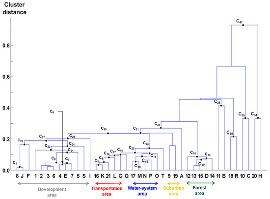
Figure 5. Dendrogram constructed based on agglomerative hierarchical clustering of the coordinates of the land-use record and category of Seoul city as per Table 1 using the proposed method.

• C₁ (8:J): Although a small portion of “8 (industrial building)” are located in “J (Warehouse site)”, these two feature classes have the closest embedded coordinates, as shown in Figure 4. This is because the proposed method performs data normalization in the form of relative frequency, as in Equation (11). Thereafter, “F (Factory site)” is clustered sequentially to process the cluster into C₂₆
• C₈ ({2,3,4,6,7}:E): Seoul city is a typical megacity and the capital of the Republic of Korea with a population equal to approximately 10 million, therefore, there are so many residential buildings constructed on the land with land-use category registered as “E (Building site)”. It should be noted that, according to its high land price, detached houses are not popular in the city, except suburban areas. Thus, C₈ represents this residence characteristic of the city.
• C₂₁ ({2,3,4,5,6,7}:E), C₂₂ ({1,2,3,4,5,6,7}:E): During the clustering process, “5 (commercial building)” and “1 (detached house)” are sequentially merged into C₈. As previously explained, “1 (detached house)” is subsequently merged into the cluster after “5 (commercial building)”.
• C₂₇ ({1,2,3,4,5,6,7,8}:{E,F,J,I,S): C₂₇ is a combination of C₂₄ and C₂₆, which together constitute the main urban development area. Then, “I (Gas station)” is merged into this cluster, which seems to be an isolated land-use category in the urban development area. This is because the safety regulation and high land prices of Seoul city lead to the fact that gas stations are located at a significant distance from central residential and/or commercial sites.
• C₁₀ (17:M), C₁₆ (17:{M, N, O, P}): “17 (river)” and “M (Bank)” are firstly clustered and then, “N (River)”, “P (Marsh)”, and “O (Ditch)” are clustered to form the water-system area. In Seoul city, central and local governments have constructed the banks along most of rivers and streams to prevent flood damage, which explains why “17 (river)” and “M (Bank)” are firstly clustered together, rather than remaining as three considered land-use categories.
• C₅ (16:K): This cluster shows that in the two datasets of the land-use record and category, feature classes named “Road” represent nearly the same real-world entity, which means that they have similar geographic concepts for roads.
• C₁₄ ({16, 21}:{K, L}): “21 (miscellaneous)” and “L (Railway site)” are then merged into C₅.
• C₂₀ ({16, 17, 21}:{G, K, L, Q, M, N, P, O}): C₂₀ is a combination of C₁₈ and C₁₉ which represents a so-called trans-hydro network. In an urban area such as Seoul city, many small streams have been covered to construct more roads as a part of the continuous urbanization process. In this process, the original land-use category of many land parcels have not been properly changed according to the substantive land-use condition. The inclusion of “G (School site)” seems to be erroneous. In Table 1, there is no proper land-use record class for educational facilities, and this means that the UIS does not manage these facilities. This is due to the fact that according to the Korean administrative legal system, the management of elementary school, middle school, and high school should be governed by local education offices, and not by the local government; therefore, the relevant data is not sufficiently reflected in the UIS, which is managed by local governments.
• C₁₅ ({12,13,14,15}:D): This cluster represents the forest area.
• C₃₆ (11:B)_, C₂₉ (18:R)_, C₃₅ (10:C), C₃₄ (20:H): These clusters represent paddy fields, parks, orchards, and parking lot areas, respectively.

Table 3 shows the clusters in Figure 5 and their F-measure with Equation (16). The above cluster analysis does not consider a quantitative criterion. In Table 3, some feature class–set pairs such as C₁, C₈, and C₂₁ have low F-measure values; meanwhile, other pairs such as C₅, C₉, C₁₂ have high values. When the proposed method is applied to identify exact corresponding feature class–set pairs, a proper F-measure threshold needs to be determined. In the case of Table 3, 0.700 seems to be such a threshold, considering the above analysis. However, the determination of this threshold requires sufficient statistical experiments. The following feature class–set pairs have been identified for the Jeonnam Province:

Table 3. Feature class–set pairs in Figure 5 and their F-measures.

No	Feature Class-Set Pair	F-Measure	No	Feature Class-Set Pair	F-Measure
C1	{8}:{J}	0.003	C20	{16,17,21}:{G,K,L M,N,O,P}	0.772
C2	{3,6}:Null		C21	{2,3,4,5,6,7}:{E}	0.586
C3	{2,3,6}: Null		C22	{1,2,3,4,5,6,7}:{E}	0.964
C4	{13,15}: Null		C23	{16,17,21}:{G,K,L M,N,O,P,Q,T}	0.773
C5	{16}:{K}	0.734	C24	{1,2,3,4,5,6,7}:{E,S}	0.964
C6	{4}:{E}	0.056	C25	{9,19}: Null
C7	{4,7}:{E}	0.251	C26	{8}:{F,J}	0.283
C8	{2,3,4,6,7}:{E}	0.433	C27	{1,2,3,4,5,6,7,8}:{E,F,J,S}	0.966
C9	{16,21}:{K}	0.732	C28	{1,2,3,4,5,6,7,8}:{E,F,I,J,S}	0.967
C10	{17}:{M}	0.163	C29	{18}:{R}	0.569
C11	{Nan}:{35,37}		C30	{1,2,3,4,5,6,7,8,16,17,21}:{E,F,G,I,J,K,L,M,N,O,P,Q,S,T}	0.987
C12	{13,15}:{D}	0.703	C31	{1,2,3,4,5,6,7,8,9, 16,17,19,21}:{E,F,G,I,J,K,L,M,N,O,P,Q,S,T}	0.979
C13	{13,14,15}:{D}	0.730	C32	{1,2,3,4,5,6,7,8,9,16,17,19,21}:{A,E,F,G,I,J,K,L,M,N,O,P,Q,S,T}	0.987
C14	{16,21}:{K,L}	0.739	C33	{1,2,3,4,5,6,7,8,9,12,13,14,15,16,17,19,21}:{A,D,E,F,G,I,J,K,L,M,N,O,P,Q,S,T}	0.992
C15	{12,13,14,15}:{D}	0.735	C34	{20}:{H}	0.493
C16	{17}:{M,N,P}	0.464	C35	{10}:{C}	0.288
C17	{16,21}:{G,K,L}	0.740	C36	{11}:{B}	0.424
C18	{16,21}:{G,K,L,Q}	0.741		⋮
C19	{17}:{M,N,O,P}	0.422	C40	All:All	1.000

• C’1 (17:N): In the clustering process, the first pair of feature classes identified is “17 (river)” and “N (River)”. In the previous clustering analysis performed for Seoul city, it had a low weight (125/577 = 0.22) according to Equation (11), however, it has a high weight (6083/8225 = 0.74) for the Joennam Province. This is because, in urban areas such as Seoul city, many roads are constructed along rivers or banks; however, in rural areas such as the Jeonnam Province, river-side areas are reserved undeveloped; consequently, the above feature classes are clustered firstly.
• C’21 (17:{M, N, O, P}): Although the order of clustering is different, the result of the analysis is similar to that of Seoul city. It can be confirmed that the 1:N feature class correspondence is the same for the city and the province; however, there is a difference in the correspondence priority of the sub-feature class depending on the regional characteristics.
• C’16 (11:B), C’14 (9:A): Unlike for Seoul city, the cluster order of the feature class related to the agricultural land was higher than that of Seoul city owing to the characteristics of the Jeonnam Province, which has a very high proportion of agricultural land. In other words, it can be confirmed that the actual land-use is performed in the same form as the land plan related to agriculture.
• C’17 (19:G): It shows that various physical education facilities other than educational buildings are installed and operated on the school site. It can be confirmed that physical education facilities are being promoted in connection with the development of school grounds being driven by the welfare projects organized by the local community.
• C’25 ({1, 9, 11, 19, 21}:{A, B, G, T}): This cluster represents the suburban and agriculture area, where “G (School site)” and “T (Miscellaneous)” are included. This is explained by the data management problem similar to that of Seoul city, or by the fact that many sports or agricultural facilities are constructed in the closed school sites in old villages.
• C’13 (16:{K, L}), C’15 (16:{K, L, Q}): Similar to the aforementioned analysis result for Seoul city, “16 (road)” and “K (Road)” were firstly clustered; however, unlike the result for Seoul city, “21 (miscellaneous)” was clustered in the suburban and agriculture area, not the transportation area.
• C’18 ({12,13,14,15}:D): This cluster represents the forest area, similarly to that in the aforementioned case for Seoul city.
• C’36 (8:F), C’33 (10:C), C’34 (18:R): These clusters represent industrial/factory, orchard, park areas, respectively.

The above clustering sequence describes local characteristics because even though they have the same land category, the results of substantive land development or land-use could be different across the regions. Figure 6 shows such a difference clustering result of the Jeonnam Province data in Table 2.

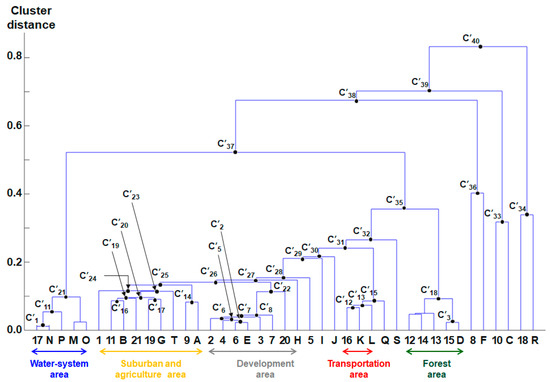
Figure 6. Dendrogram constructed based on agglomerative hierarchical clustering of the coordinates of the land-use record and category in the Jeonnam Province data as per Table 2, using the proposed method.

Table 4 shows F-measure values of the clusters in Figure 6, similar to Table 3. Comparing to Table 3, the clusters related to suburban and agriculture areas, such as C’₁₄ and C’₁₆, have high F-measure values. Meanwhile, those related to the development area, such as C’₅, C’₆, C’₇, and C’₈, have low values.

Table 4. Feature class–set pairs in Figure 6 and their F-measures.

No	Feature Class-Set Pair	F-Measure	No	Feature Class-Set Pair	F-Measure
C’1	{17}:{N}	0.247	C’18	{12,13,14,15}:{D}	0.933
C’2	{6}:{E}	0.009	C’19	{11,21}:{B}	0.937
C’3	{15}: {D}	0.015	C’20	{11,19,21}:{B,G}	0.936
C’4	Null:{M,O}		C’21	{17}:{M,N,O,P}	0.702
C’5	{4,6}:{E}	0.013	C’22	{2,3,4,6,7,20}:{E}	0.100
C’6	{2,4,6}:{E}	0.016	C’23	{11,19,21}:{B,G,T}	0.934
C’7	{2,3,4,6}:{E}	0.018	C’24	{1,11,19,21}:{B,G,T}	0.768
C’8	{2,3,4,6,7}:{E}	0.099	C’25	{1,9,11,19,21}:{A,B,G,T}	0.864
C’9	{12,14}:Null		C’26	{1,2,3,4,7,6,9,11,19,20,21}:{A,B,E,G,T}	0.965
C’10	{12,13,14}:Null			⋮
C’11	{17}:{N,P}	0.493	C’33	{10}:{C}	0.408
C’12	{16}:{K}	0.742	C’34	{18}:{R}	0.384
C’13	{16}:{K,L}	0.747	C’35	{1,2,3,4,5,6,7,9,11,12,13,14,15,16,19,20,21}:{A,B,D,E,G,H,I,J,K,L,Q,ST}	0.993
C’14	{9}:{A}	0.897	C’36	{8}:{F}	0.596
C’15	{16}:{K,L,O}	0.750		⋮
C’16	{11}:{B}	0.938	C’40	All:All	1.000
C’17	{19}:{G}	0.207

Considering the above analysis results provided for Seoul city and the Jeonnam Province, the characteristics of the proposed method could be identified as follows. First, it is possible to explore the various semantic correspondences of the feature classes through analyzing the clustering order in the embedded space. Adjacent feature classes in the space share more spatial objects, which means that they have a high probability to represent the same real-world entity or phenomena. According to the assumptions of this research and many previous related studies, these feature classes can be classified as semantically corresponding pairs. Therefore, applying agglomerative hierarchical clustering, hierarchical semantic relations of the feature classes such as “is_subset_of”, “is_superset_of”, or “is_same_to” could be obtained, similarly to [13].

Second, it is possible to infer regional characteristics of the feature classes. For example, the lands for which the land-use category is T (Miscellaneous) were generally used for the transportation area in Seoul city, and for the suburban and agricultural areas in the Jeonnam Province, as shown in Figure 4 and Figure 5, respectively. This is because there is high land development demand for transportation services in urban areas such as Seoul city. However, in the Jeonnam Province, where only a small part of its area is urbanized, there is no specific land development demand, and thus, the lands for which the land-use category is T (Miscellaneous) were developed in various forms. However, the water-system area and the forest area showed very similar clustering results. This can be explained by the natural environment protection due to the intervention of the central government, which results in similar land development tendencies for both urban and rural areas.

5. Conclusions

In this article, we proposed a new method to identify semantic correspondences between two datasets by means of finding hierarchical M:N corresponding feature class–set pairs. Applying the overlapping analysis to the object sets within the feature classes, the similarities of the feature classes are estimated and projected onto a lower-dimensional vector space after applying the graph embedding method. Thereafter, as the feature classes of high similarity are distributed close to each other in the projection space, distance-based clustering is conducted to identify the semantically corresponding feature class pairs. The above method was applied to the cadastral parcels’ land-use record in UIS and the corresponding land-use category in KLIS for two different test sites, Seoul city and the Jeonnam Province. As a result, it was possible to find various semantic correspondences of the feature classes between UIS and KLIS. In addition, hierarchical structures of the correspondences could be obtained. Moreover, upon analyzing these structures to obtain sequential clustering orders, regional characteristics of the feature classes were also inferred.

The proposed method is based only on the results of the overlay analysis between datasets. Therefore, aside from the location information, other prior information related to the construction of similarity measures was not required. This is an advantage in terms of generality as the proposed method can be applied to various geospatial datasets. Moreover, an advanced method could be developed by combining various similarity measures, such as lexical similarity, structural similarity, category similarity, shape similarity, and so on [18,28,29] into the co-occurrence matrix, in which rows and columns represent entities under analysis, such as feature classes in this study. To combine these various similarity measures between these entities, it is necessary to determinate their weight. We will consider these aspects to improve the proposed method in future studies.

References

- Vaccari, L.; Shvaiko, P.; Marchese, M. A geo-service semantic integration in spatial data infrastructures. Int. J. Spat. Data Infra. 2009, 4, 24–51. [Google Scholar]
- Uitermark, H.T.; van Oosterom, J.M.; Mars, N.J.I.; Molenaar, M. Ontology-based integration of topographic data sets. Int. J. Appl. Earth Obs. 2005, 7, 97–106. [Google Scholar] [CrossRef]
- Khatami, R.; Alesheikh, A.A.; Hamrah, M. A mixed approach for automated spatial ontology alignment. J. Spat. Sci. 2010, 55, 237–255. [Google Scholar] [CrossRef]
- Ruiz-Casado, M.; Alfonseca, E.; Castells, P. From Wikipedia to Semantic Relationships: A Semi-automated Annotation Approach. In Proceedings of the Third Annual European Semantic Web Conference ESWC’06, Budva, Montenegro, 12 June 2006. [Google Scholar]
- Ruiz, J.J.; Ariza, F.J.; Ureña, M.A.; Blázquez, E.B. Digital map conflation: A review of the process and a proposal for classification. Int. J. Geogr. Inf. Sci. 2011, 25, 1439–1466. [Google Scholar] [CrossRef]
- Kokla, M. Guidelines on geographic ontology integration. In Proceedings of the ISPRS Technical Commission II Symposium, Vienna, Austria, 12–14 July 2006. [Google Scholar]
- Rodríguez, M.A.; Egenhofer, M.J.; Rugg, R.D. Assessing Semantic Similarities among Geospatial Feature Class Definitions. In Lecture Notes in Computer Science Vol. 1580; Včkovski, A., Brassel, K.E., Schek, H.J., Eds.; Springer: Berlin, Germany, 1999; pp. 189–202. [Google Scholar]
- Duckham, M.; Mason, K.; Stell, J.; Worboys, M. A formal approach to imperfection in geographic information. Comput. Environ. Urban Syst. 2001, 25, 89–103. [Google Scholar] [CrossRef]
- Duckham, M.; Worboys, M. An algebraic approach to automated geospatial information fusion. Int. J. Geogr. Inf. Sci. 2005, 19, 537–557. [Google Scholar] [CrossRef]
- Cruz, I.F.; Sunna, W. Structural Alignment Methods with Applications to Geospatial Ontologies. Trans. GIS 2008, 12, 683–711. [Google Scholar] [CrossRef]
- Buccella, A.; Cechich, A.; Gendarmi, D.; Lanubile, F.; Semeraro, G.; Colagrossi, A. Building a global normalized ontology for integrating geographic data sources. Comput. Geosci. 2011, 37, 893–916. [Google Scholar] [CrossRef]
- Bhattacharjee, S.; Ghosh, S.K. Measuring semantic similarity between land-cover classes for spatial analysis: An ontology hierarchy exploration analysis. Innov. Sys. Softw. Eng. 2016, 12, 193–200. [Google Scholar] [CrossRef]
- Kuo, C.L.; Hong, J.H. Interoperable cross-domain semantic and geospatial framework for automatic change detection. Comput. Geosci. 2016, 86, 109–119. [Google Scholar] [CrossRef]
- Kuai, X.; Li, L.; Luo, H.; Hang, S.; Zhang, Z.; Liu, Y. Geospatial Information Categories Mapping in a Cross-lingual Environment: A Case Study of “Surface Water” Categories in Chinese and American Topographic Maps. ISPRS Int. J. Geo. Inf. 2016, 5, 90. [Google Scholar] [CrossRef]
- Zhang, Y.; Yang, P.; Li, C.; Zhang, G.; Wang, C.; He, H.; Hu, X.; Guan, Z. A multi-feature based automatic approach to geospatial record linking. Int. J. Semt. Web Inf. Sys. 2018, 14, 73–91. [Google Scholar] [CrossRef]
- Huang, Y. Conceptual categorizing geographic features from text based on latent semantic analysis and ontologies. Ann. GIS 2016, 22, 113–127. [Google Scholar] [CrossRef][Green Version]
- Sedoc, J.; Gallier, J.; Ungar, L.; Foster, D. Semantic word clusters using signed normalized graph cuts. arXiv 2016, arXiv:1601.05403. [Google Scholar]
- Sun, K.; Zhu, Y.; Song, J. Progress and Challenges on Entity Alignment of Geographic Knowledge Bases. ISPRS Int. J. Geo. Inf. 2019, 8, 77. [Google Scholar] [CrossRef]
- Hendrickson, B. Latent semantic analysis and Fiedler embedding. Linear. Algebra Appl. 2007, 421, 345–355. [Google Scholar] [CrossRef][Green Version]
- Huh, Y.; Kim, J.; Lee, J.; Yu, K.; Shi, W. Identification of multi-scale corresponding object-set pairs between two polygon datasets with hierarchical co-clustering. ISPRS J. Photo. Rem. Sens. 2014, 88, 60–68. [Google Scholar] [CrossRef]
- Belkin, M.; Niyoki, P. Laplacian eigenmaps for dimensionality reduction and data representation. Neural Comp. 2003, 15, 1373–1396. [Google Scholar] [CrossRef]
- Sameh, A.; Wisniewski, J. A trace minimization algorithm for the generalized eigenvalue problem. SIAM J. Num. Anal. 1982, 19, 1243–1259. [Google Scholar] [CrossRef]
- Min, D.; Zhilin, L.; Xiaoyong, C. Extended Hausdorff distance for spatial objects in GIS. Int. J. Geogr. Inf. Sci. 2007, 21, 459–475. [Google Scholar] [CrossRef]
- Li, L.; Goodchild, M. An optimisation model for linear feature matching in geographical data conflation. Int. J. Image Data Fus. 2011, 2, 309–328. [Google Scholar] [CrossRef]
- Dhillon, I. Co-clustering documents and words using bipartite spectral graph partitioning. In Proceedings of the 7th ACM SIGKDD International Conference on Knowledge Discovery and Data Mining, San Francisco, CA, USA, 26–29 August 2001. [Google Scholar]
- Cho, M.; Lee, J.; Lee, K. Feature correspondence and deformable object matching via agglomerative correspondence clustering. In Proceedings of the 12th IEEE International Conference on Computer Vision, Kyoto, Japan, 27 September–4 October 2009. [Google Scholar]
- Euzenat, J.; Shavaili, P. Ontology Matching, 2nd ed.; Springer: New York, NY, USA, 2013; p. 304. [Google Scholar]
- Van den Brink, L.; Janssen, P.; Quak, W.; Stoter, J. Towards a high level of semantic harmonisation in the geospatial domain. Comp. Environ. Urban Sys. 2017, 62, 233–242. [Google Scholar] [CrossRef]
- Yu, L.; Qiu, P.; Liu, X.; Lu, F.; Wan, B. A holistic approach to aligning geospatial data with multidimensional similarity measuring. Int. J. Dig. Earth 2018, 11, 845–862. [Google Scholar] [CrossRef]
© 2019 by the author. Licensee MDPI, Basel, Switzerland. This article is an open access article distributed under the terms and conditions of the Creative Commons Attribution (CC BY) license (http://creativecommons.org/licenses/by/4.0/).