FC-RRT*: An Improved Path Planning Algorithm for UAV in 3D Complex Environment

Abstract

In complex environments, path planning is the key for unmanned aerial vehicles (UAVs) to perform military missions autonomously. This paper proposes a novel algorithm called flight cost-based Rapidly-exploring Random Tree star (FC-RRT*) extending the standard Rapidly-exploring Random Tree star (RRT*) to deal with the safety requirements and flight constraints of UAVs in a complex 3D environment. First, a flight cost function that includes threat strength and path length was designed to comprehensively evaluate the connection between two path nodes. Second, in order to solve the UAV path planning problem from the front-end, the flight cost function and flight constraints were used to inspire the expansion of new nodes. Third, the designed cost function was used to guide the update of the parent node to allow the algorithm to consider both the threat and the length of the path when generating the path. The simulation and comparison results show that FC-RRT* effectively overcomes the shortcomings of standard RRT*. FC-RRT* is able to plan an optimal path that significantly improves path safety as well as maintains has the shortest distance while satisfying flight constraints in the complex environment. This paper has application value in UAV 3D global path planning.

1. Introduction

In the last decade, unmanned aerial vehicles (UAVs) have gradually come to play an important role in various military operations [1]. UAVs can greatly improve the threat target surprise defense capability, battlefield speed escape capability, hostile fire suppression capability, and multi-dimensional diversified combat capability. Path planning is one of the most important problems that can take place during the autonomous navigation flight of UAVs [2,3], which is usually defined as autonomously finding an optimal path from the start node to the end node [4]. Optimal path selection needs to be determined based on the flight performance constraints, the specific mission requirements, and the flight environment constraints [5,6]. Scholars have conducted a lot of research on the UAV path planning problem and proposed a series of algorithms, such as graph-based optimization methods, including the visibility graph (VG) algorithm [7] and Voronoi diagrams [8]; the searching-based methods, including the Dijkstra [9] algorithm, A* algorithm [10] and D* algorithm [11]; the sampling-based methods, such as PRM algorithm [12] and RRT algorithm [13]; the nature-inspired methods, such as genetic algorithm (GA) [14], ant colony optimization (ACO) [15], artificial potential field algorithm [16], particle swarm optimization (PSO) [17] and fluid-based algorithm [18]; and other methods, such as control theory-based methods [19].

As a sampling-based path planning algorithm, RRT* does not explicitly construct the entire planning space and its boundaries as a searching-based method, but instead directly obtains samples through sampling to form a search tree. This approach avoids the problem where search time grows exponentially with the number of spatial dimensions, thus significantly reducing the search time available for path planning in high-dimensional spaces [20,21]. Meanwhile, compared to intelligent methods, such as GA and ACO, RRT* has a lower algorithmic complexity in 3D space [22,23]. As such, it is more suitable for solving path planning problem in 3D space. Additionally, RRT* has been proven to be asymptotically optimal. In other words, when the number of samples tends to infinity, the solution that is obtained by RRT* is the optimal solution that converges with the probability solution [24]. Therefore, for UAV path planning in a complex environment, RRT* can ensure that a feasible path in 3D space is found quickly. In summary, RRT* is more suitable for UAV path planning than other algorithms in complex environments.

Recent research developments have proposed many improved RRT* algorithms using different approaches to improve the performance of RRT*. On the one hand, some scholars use biasing sampling to improve RRT* [25,26,27,28]. This approach attempts to distribute the samples in the favorable region through the biasing procedure, such as Theta*-RRT* [27] and A*-RRT* [28]. Although this approach can improve the initial sampling quality and the convergence speed of the algorithm, the planning path cannot satisfy the flight and environmental constraints of the UAV. On the other hand, some improved RRT* algorithms based on heuristic information to guide local sampling have also been proposed [29,30,31,32]. These algorithms will use heuristic information to guide the search after RRT* finds a feasible path for the first time in order to find the optimal path quickly. In addition to the two improved approaches mentioned above, there is another approach that can be implemented to improve RRT* performance, which the relaxation of asymptotic optimality [33,34,35], such as through the LBT-RRT proposed by Salzman [33]. The path that is obtained by this algorithm eventually converges with the probability one to a path within a factor of $(1+\epsilon )$ of the optimal path, so it is called asymptotically near-optimal. Compared to RRT, this algorithm produces high-quality solutions faster and the quality of the solutions is essentially comparable to those of RRT* or RRG. Other algorithms that use this improved approach are SST [34] and NoD-RRT [35]. These approaches can effectively improve the performance of RRT*, but the solution is asymptotically near-optimal.

It is not difficult to determine that the improved RRT* algorithms by these three different approaches are not suitable for UAV path planning because they take into account neither the impact of complex environments on the path safety of UAVs nor the flight constraints. Note that in this paper, path safety refers to how when the path of the UAV is affected by threats with detection or attack range, the planned path makes it possible for the UAV to avoid being threatened, ensuring its safety. If the path safety and flight constraints determined by a complex environment are considered after the optimal path is generated using these improved algorithms, then the optimality of the final path will be affected, and it is possible that even a feasible path may not be found. Therefore, for UAV path planning and optimization in complex 3D environments, the impact of various threats on path safety and the flight constraints should be fully considered when finding the optimal path in order to ensure that the final planning path is the optimal path that satisfies both the safety and flight constraints. In the sparse A* algorithm [36], the authors considered the flight constraints when searching the space, making it possible to obtain a flyable optimal path while greatly reducing the search range and complexity. Similarly, in some evolutionary algorithms [37,38], the threat impact of the complex environment and flight constraints are also included in the objective function in order to directly plan the optimal path by satisfying the path safety and constraints. However, few improvements making UAV path planning suitable in complex environments have been seen for the RRT* algorithm.

For the flight mechanics constraints of UAVs, two studies, [37,39], provide some typical flight constraints for UAV path planning. Most of these constraints are concentrated on the geometric level to constrain the path points in the planned path (such as the angle constraints of the UAV, etc.). If only the length of the planned path is used as the standard for path evaluation, then these constraints are feasible. However, in this paper, we also need to consider the path threat cost of UAVs. It is not feasible to evaluate the path threat cost by relying on the path points alone. Occasionally, there are situations where the adjacent path points meet the constraints, but the path segments do not. Therefore, this paper makes some improvements to the flight constraints in [37,39]. For some constraints that need to be evaluated on the path segment, consider whether the path segment conflicts with the constraint while the path point meets the constraint.

Therefore, for UAV path planning problems in complex military operational environments, this paper proposes a new algorithm called FC-RRT*, which is inspired by the sparse A* and the improved evolutionary algorithms. We designed a flight cost function that use the distance cost and threat cost as the basis of FC-RRT*. In the extension of the tree nodes, we consider the flight cost function and flight constraints comprehensively and use them as heuristic information to guide the expansion of the tree nodes. After that, the flight cost function and flight constraints are also used to guide the update of the parent nodes. By guiding the flight cost function and flight constraint together twice, an algorithm is created to find an optimal path with the shortest length and that satisfies path safety and flight constraints. The path satisfies the planning requirements of military operations, such as surveillance and reconnaissance, hostile fire suppression capability, battlefield speed escape capability, and threat-target surprise defense capability. The contributions can be summarized as follows in Figure 1:

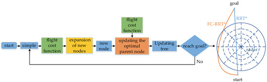
Figure 1. Flowchart and result diagram of FC-RRT * algorithm. In the figure, the green box represents contribution 1, the yellow box represents contribution 2, and the orange box represents contribution 3. It can be seen in the result diagram that the algorithm in this paper can obtain a path with higher path safety for radar and other threat areas than RRT* can.

• A flight cost function including threat strength and path length was established to improve the UAV path safety in complex environments. Path safety is one of the most important requirements in UAV path planning. Therefore, it is not adopted to judge the path using Euclidean distance alone. Considering this problem, a flight cost function that includes path length and threat strength is proposed to guide the path planning of the UAV. This enables the UAV to effectively avoid threats and to improve its path safety by obtaining the shortest path.
• This paper proposes an approach to guide the expansion of new nodes using heuristic information. To solve the threat strength problem in UAV path planning from the front-end, both path length and threat strength cost as well as flight constraints should be considered when the FC-RRT* performs new node expansion. Therefore, we propose an approach that uses the flight cost function as heuristic information to directly guide node expansion while introducing flight constraints to it for the first time. Moreover, the algorithm structure is optimized to improve the operation efficiency of FC-RRT*. Using this approach, the path threat strength is reduced from the initial new node expansion to guarantee the path safety of the UAV. In addition, FC-RRT* also leads to less sample dispersion in the planning space.
• This paper proposes a new approach for updating the optimal parent node in the neighbor region. After the new node is guided by the flight cost function and flight constraints, an approach of introducing the flight cost function and flight constraints to update the parent node is proposed to guide optimal path finding. This approach selects the parent nodes with the shortest path length and can effectively avoid threats when updating the parent node in order to avoid being discovered by the enemy or colliding with obstacles and ensuring path safety.

The rest of this paper is organized as follows: Section 2 describes the UAV path planning in complex environments, laying the foundation for the current work. Section 3 analyzes the FC-RRT* algorithm in detail from five aspects: FC-RRT* framework; the determination of the flight cost function; the path evaluation criteria; the new node selection approach, which is guided by heuristic information; and the improved parent node update approach. Section 4 analyzes FC-RRT*, including its probabilistic completeness and asymptotic optimality, and compares its asymptotic computational complexity with RRT*. The simulation and comparison results are discussed in Section 5. Section 6 contains the conclusions and future prospects.

2. Related Work and Problem Description

We briefly summarize the A* algorithm, RRT algorithm, and RRT* algorithm as the description of relevant work in Section 2.1. Then, the problems to be described in this paper are analyzed and discussed in Section 2.2.

2.1. Related Work

The A* algorithm is a classic shortest path search algorithm that is based on the Dijkstra algorithm. The search direction is determined by introducing the distance heuristic information from the node to the end point in the node expansion process in order to improve the search efficiency and to shorten the search time. The A* algorithm measures the possibility that node $n$ is the point on the shortest path determined through an estimation function $f\left(n\right)$ during node expansion. The valuation function $f\left(n\right)$ can be expressed as $f\left(n\right)=g\left(n\right)+h\left(n\right)$, where $g\left(n\right)$ represents the actual cost from the initial node to node $n$, and $h\left(n\right)$ represents the estimated cost from node n to the target node. As the heuristic term is related to the target node, the node search direction in the A* algorithm is directed to the target point in order to improve the search efficiency.

The RRT algorithm takes the starting point as the root node and constructs a fast search tree composed of feasible path segments incrementally. At the beginning of the algorithm, a search tree is constructed using only the initial node as the root node. First, the expansion target point $x_{rand}$ is determined by random sampling, and then, the leaf node $x_{nearest}$ closest to $x_{rand}$ is found from the nodes of the current tree. If the distance between $x_{rand}$ and $x_{nearest}$ is within a certain range, then $x_{rand}$ is taken as the new node $x_{new}$; otherwise, select a node within a certain range around the leaf node in the $x_{rand}$ direction to be $x_{new}$. Then, try to connect $x_{new}$ into the tree. If the connection between $x_{new}$ and $x_{nearest}$ does not collide with the environmental obstacles, connect $x_{new}$ into the search tree as a new leaf node. When the leaf node of the random tree contains the goal or is in the area around the goal, a path from the start to the goal that is composed of tree nodes can be found in the random tree.

Compared to the RRT * algorithm, the RRT algorithm increases the optimization process when connecting sampling points during the search tree. The parent node selection method for $x_{new}$ is as follows: find the set $X_{near}$ of all of the nodes $x_{near}$ within a certain distance of $x_{new}$ and then select the point in $X_{near}$ that can be connected with $x_{near}$ without collision and that has the shortest length as the parent node. Then, $x_{near}$ near $x_{new}$ is reviewed in the tree. When the path from $x_{near}$ to $x_{new}$ is shorter, remove the connection between $x_{near}$ and the parent node, and set the parent node of these points as point $x_{new}$.

2.2. Problem Description

In real flight environments where UAVs are performing military operations, there will usually be many types of obstacles and threats, including terrain threats, radar threats, anti-aircraft gun threats, and no-fly zone threats. Different types of threats are handled in different ways. Therefore, in order to truly restore the UAV flight environment, this paper simulates a complex environment containing the above threats and plans the UAV path in this environment. The definition of a complex environment in this paper is as follows:

Definition 1 (complex environment)

. If the environment in which the UAV path planning takes place is a three-dimensional space with terrain threats, radar threats, anti-aircraft gun threats, and no-fly zone obstacles, and the same type of threat occurs many times, then the UAV path-planning environment is defined as being complex.

The definition and modeling of different types of obstacles in a complex space are also different. They are analyzed below:

(1) Terrain threats: Due to the large topographic relief, more information will be lost if it is approximately represented by the basic configuration. As such, it is difficult to represent this topographic information using the basic configuration. In order to accurately represent terrain information and to improve operation efficiency, we note that the elevation data are mostly stored in the lattice, so it is easy to convert the elevation data into a three-dimensional grid environment model. Therefore, this paper uses the elevation map information for Hawaii Island as the terrain threat.

(2) Radar threats and anti-aircraft gun threats: Radar threats and anti-aircraft gun threats cannot be treated as a no-fly zone. This is because radar and anti-aircraft gun threats have both detection range and attack range. It is not enough to avoid the threat itself, which will bring hidden dangers to path security. Therefore, when avoiding such threats, it is also necessary to stay as far away from the treat center as possible in order to reduce the degree of the threat that a UAV experiences when crossing the radar detection range or anti-aircraft gun attack range and to ensure the path safety of UAV to a certain extent.

(3) No-fly zone obstacles: To avoid the obstacles in the no-fly zone, we simulated tower obstacles. For such obstacles, if a UAV has planned a path that allows it to successful avoid colliding with them, then the UAV has successfully avoided such obstacles.

These complex environmental conditions and UAV performance bring many flight constraints to path planning. A careful look at the constraints of UAV path planning problems shows that most of them are constrained at the geometric level by using separated route points (path planning generally does not consider dynamic constraints). Since this paper focuses on the UAV path planning problem rather than constructing new flight constraints, we directly select and derive a set of flight constraints suitable for this paper based on the existing representative constraints in [37,39] to accommodate the key performance constraints and complex environmental requirements in UAV path planning.

The constraints are calculated as follows.

1.

Path length constraint

The path length is used to represent the flight distance of the UAV. Let $L_{\max }$ be the maximum flight distance of the UAV. Then, the path length constraint is calculated as

$$f_L={\displaystyle \sum _{i=0}^N\sqrt{{(x_{i+1}-x_i)}^2+{(y_{i+1}-y_i)}^2+{(z_{i+1}-z_i)}^2}}\le L_{\max }$$

(1)

where $(x_i,y_i,z_i)$, $i=1,2,\dots ,N$, denotes the coordinate of the $i$-th path point in the 3D planning environment, and $N$ is the total number of path points.

2.

Turning angle constraint

Consider the smoothness of the path, where the maximum turning angle ${\varphi }_{\max }$ is introduced to constrain the turning angle. Suppose the vector $a_i$ is equal to ${[x_i-x_{i-1},y_i-y_{i-1},]}^T$, and $\left|\right|a_i\left|\right|$ is the norm of vector $a_i$. The turning angle constraint of UAV is

$${\varphi }_i=\arccos (\frac{a_i^T{a}_{i+1}}{\left|\right|a_i\left|\right| \left|\right|a_{i+1}\left|\right|})\le {\varphi }_{\max }$$

(2)

3.

Climbing/gliding angle constraint

Similar to the turning angle, the climbing/gliding angle can be calculated as

$$-{\gamma }_{\max }\le {\gamma }_i=\arctan (\frac{z_i-z_{i-1}}{\left|\right|a_i\left|\right|})\le {\gamma }_{\max },$$

(3)

where ${\gamma }_{\max }$ is the maximum climbing angle, and the $-{\gamma }_{\max }$ is the minimum gliding angle.

4.

Path segment constraint

The UAV must maintain a direct distance before changing the flight attitude or after turning. Additionally, UAVs do generally not expect to turn frequently in order to reduce navigation errors. Therefore, it is necessary to limit the path segments between adjacent path points to be larger than the shortest path segment length $l_{\min }$. The path segment constraint can be expressed by

$$l_{\min }-\left|\right|p_{i+1}-p_i\left|\right|\le 0,$$

(4)

where $p_{i+1}$ is $(x_{i+1},y_{i+1},z_{i+1})$, and $p_i$ is $(x_i,y_i,z_i)$. $p_{i+1}$ and $p_i$ are two adjacent path points.

5.

Terrain limit

To calculate the terrain constraints, relying on path points alone may cause the corresponding path segments to collide with the terrain, so the constraints of the path segments also need to be considered. Hence, let $p_{i,k}$ be any path point on the path segment $(p_i,p_{i+1})$; $H_{safe}$ is the minimum safe flight altitude of the UAV, and $z_{i,j}^{map}$ is the terrain altitude at path point $p_{i,k}$. Then, the terrain limit is

$$g_{1,j}=\{\begin{array}{l}0 p_{i,j}\ge H_{safe}+z_{i,j}^{map}\\ 1 \mathrm{otherwise}\end{array}$$

(5)

We usually use the path length as a cost function to evaluate the planned paths. However, in this paper, which considers the impact of complex environmental factors on the path safety of the UAV, the distance between the path and the threat area is also considered to avoid planning a path that is too close to the threat, which is expressed through the path threat strength cost function. In Section 3, we will analyze the cost function in detail.

3. FC-RRT* Algorithm

The standard RRT* approximates the search space by sampling, avoiding the sharp increase in computational complexity caused by the increase in the dimensionality of the search space. Therefore, it is suitable for UAV path planning. However, studies [40,41] proved that the standard RRT* cannot guarantee the path safety of UAVs in path planning and that may even make the path infeasible due to the violation of flight constraints.

Therefore, considering the path safety and flight constraints of UAVs in complex environments, a new algorithm, named FC-RRT*, is proposed in this paper to find the optimal UAV path. Firstly, a flight cost function is designed using the threat strength and path length; secondly, the designed flight cost function and flight constraint are used to guide the expansion of new nodes directly. Finally, the designed flight cost function and flight constraint are used to guide the update of the parent nodes in the neighboring regions. FC-RRT* considers threat strength and path length at the same time. Its purpose is to plan an optimal path that is as short as possible while also effectively avoiding the threat, in order to satisfy UAV path planning requirements for military operations in complex environments (Algorithm 1 is FC-RRT* framework).

Algorithm 1: FC-RRT*

$\begin{array}{l}1:\hspace{1em}\mathbf{Notation}: \mathrm{Tree} T, \mathrm{Enviroment} \xi \\ 2:\hspace{1em}T.V\leftarrow \left\{p_{start}\right\}; E\leftarrow \varnothing ;\\ 3:\hspace{1em}\mathbf{for} i=1 \mathrm{to} n \mathbf{do}\\ 4:\hspace{1em}\hspace{0.17em} T\leftarrow (V,E);\\ 5:\hspace{1em}\hspace{0.17em} p_{rand}\leftarrow \mathrm{Sample}(\xi );\\ 6:\hspace{1em}\hspace{0.17em} p_{new}\leftarrow \mathrm{Heuristic}\_\cos \mathrm{t}(T.V,p_{rand})\\ 7:\hspace{1em}\hspace{0.17em} T.V\leftarrow T.V\cup \left\{p_{new}\right\};\\ 8:\hspace{1em}\hspace{0.17em} P_{near}\leftarrow \mathrm{Near}(p_{new},T.V,r_i);\\ 9:\hspace{1em}\hspace{1em} \mathbf{for} all p_{near}\in P_{near} \mathbf{do}\\ 10:\hspace{1em}\hspace{1em}\hspace{1em} \mathrm{rewire}\_\mathrm{ImpRRT}*(p_{near},p_{new});\\ 11:\hspace{1em}\hspace{0.17em}\hspace{0.17em} \mathbf{for} all p_{near}\in P_{near} \mathbf{do}\\ 12:\hspace{1em}\hspace{1em}\hspace{1em} \mathrm{rewire}\_\mathrm{ImpRRT}*(p_{new},p_{near});\\ 13: \mathbf{return} T=(V,E)\end{array}$

The FC-RRT* as given in Algorithm 1 differs from the standard RRT* in two parts: the expansion of new nodes and the update of the parent nodes in the neighboring regions. For the new node expansion, RRT * first selects the node in the tree that is the closest to the sample node. Then, a new node is selected in the direction of the tree node to the sample node according to the expansion distance. Finally, if the new node is collision-free, then it is added to the tree [24]. In contrast, our FC-RRT* algorithm uses the flight cost function as heuristic information to guide the expansion of new nodes. The heuristic information already includes guidance on the expansion direction and distance of new nodes, so new nodes satisfying the flight constraint can be added directly to the tree (Algorithm 1, lines 6, 7). To update the parent node, the Euclidean distance is usually used to select the nearest parent node without considering the threat strength and flight constraints in RRT*. In the FC-RRT* algorithm, we use the flight cost function and flight constraints to guide the selection of the optimal parent node (Algorithm 1, lines 9–12). Since this approach considers the threat strength, path length, and flight constraints simultaneously, the planned path is an optimal path that satisfies the path safety and constraints. The details of FC-RRT* are analyzed below.

3.1. Evaluation of the Flight Cost Function

For UAV path planning in a complex environment, it is not enough to only consider one path length factor. UAVs not only need to avoid the no-fly zone when flying in the battlefield, they also need to avoid the impact of threats, such as radars and anti-aircraft guns, as much as possible according to different missions. Furthermore, even if radar and anti-aircraft guns are avoided, the UAV is still be threatened by radar detection and anti-aircraft attacks, meaning that its path safety cannot be ensured. In other words, we expect the algorithm to keep the UAV away from threats while obtaining a shorter path, so as to avoid reducing the path safety of the UAV by only pursuing the shortest planned path.

Generally, the threat radius of radar and anti-aircraft guns is very large, so it would be impractical to attempt to totally avoid all of the threats that they pose. If the algorithm is designed to be completely free from these threats, then it would result in the length of the path being increased or would result in a path planned far beyond the flight environment. Therefore, we cannot simply regard these threat areas as no-fly zones that can be completely avoided. Note that the probability of being detected by radar and attacked by anti-aircraft guns decrease as the distance between the UAV and the treat increases. Therefore, it is necessary to consider the impact of the path length and path threat at the same time. Further, the impact of the path threat on mission completion is adjusted appropriately according to different UAV missions. Hence, different from the cost function of the standard RRT*, the FC-RRT* algorithm improves the original path evaluation method by using length as the only cost. In this paper, we designed a flight cost function with the threat and length cost of the path segments that can be used to guide the expansion of new nodes and to update the parent nodes. It enables the planned path to meet the UAV path requirements in complex environments. The flight cost function is analyzed in this section, which lays the foundation for the subsequent algorithm analysis.

The flight cost function contains the path length cost and the threat strength cost, defined as

$$f_c={\lambda }_l{f}_l+{\lambda }_t{f}_t,$$

(6)

where $f_l$ is the length cost of the path segment and $f_t$ is the threat cost of the path segment. ${\lambda }_l$ and ${\lambda }_t$ are the weighting factors.

3.1.1. Path Length Cost Function

To calculate the length cost of the path segment, let any pair of nodes be $p_a=(x_a,y_a,z_a)$ and $p_b=(x_b,y_b,z_b)$. The length $l$ of the path segment $(p_a,p_b)$ is

$$l=\sqrt{{(x_a-x_b)}^2+{(y_a-y_b)}^2+{(z_a-z_b)}^2}$$

(7)

Then, the length cost function $f_l$ of path segment $(p_a,p_b)$ is defined as

$$f_l(p_a,p_b)=\frac{l-l_{\min }}{l_{\max }-l_{\min }},$$

(8)

where $l_{\max }$ is the maximum distance among all of the optional path segments. Similarly, $l_{\min }$ is the minimum distance among the optional path segments.

3.1.2. Path Threat Strength Cost Function

The threat cost is the extent to which the UAV is exposed to enemy threats while flying. Obviously, the closer a UAV is to threats such as radar and anti-aircraft guns, the greater the probability that the UAV will be found or destroyed, meaning that the threat impact is stronger. Regarding the calculation of the threat strength, not only should the threat intensity at the path points be calculated, but the path segments that are connected by the path points should also be analyzed approximately. Therefore, we first processed the path segment as follows.

For a path segment $(p_a,p_b)$, divide it into $N_0$ piecewise parts uniformly. Suppose that the $j$th dividing point in the path segment $(p_a,p_b)$ is denoted as $p_{ab,j}=(x_{ab,j},y_{ab,j},z_{ab,j})$, which is calculated as

$$p_{ab,j}=\frac{p_b-p_a}{N_0}j+p_a$$

(9)

The determination of the $N_0$ value depends on the minimum threat radius and the approximate minimum diameter of the hill terrain. It is necessary to ensure that the length of all of the dividing segments is less than the minimum diameter of the radar, anti-aircraft guns and other threats. This will detect whether the path segment conflicts with threats, and there will be no situation where the path points satisfy the constraint but the path segment does not. $N_0$ is calculated as

$$\min N_0=\lceil \frac{f_L}{2N\min (r_1,\dots r_n)}\rceil ,$$

(10)

where $N$ is the number of path segments, and $r_1,\dots ,r_n$ is the minimum radius of $n$ threats or hill terrain. $f_L$ is the total path length, which is approximately 1.5 to 2 times the distance from the start to the destination. $N_0$ can also be increased according to the accuracy requirement after the minimum value constraint is satisfied. However, it should be noted that the larger the $N_0$ is, the higher the computational complexity will be.

For a path segment $(p_a,p_b)$ that is evenly divided into $N_0$ segments, the threat intensity can be expressed as

$$t=\frac{\sqrt{{(x_a-x_b)}^2+{(y_a-y_b)}^2+{(z_a-z_b)}^2}}{N_0}{\displaystyle \sum _k^K{\displaystyle \sum _j^{N_0+1}\frac{1}{d_{j,k}}}}$$

(11)

Hence, the cost function of the threat is

$$f_t(p_a,p_b)=\frac{t-t_{\min }}{t_{\max }-t_{\min }},$$

(12)

with

$$d_{j,k}=\{\begin{array}{l}\left|\right|[\frac{p_b-p_a}{N_0}(j-1)+p_a]-R_k\left|\right|-r_k\hspace{1em}{d}_{j,k}\le L_{th}\\ \hspace{1em}\hspace{1em}\hspace{1em}\hspace{1em}\hspace{1em}\infty \hspace{1em}\hspace{1em}\hspace{1em}\hspace{1em}\hspace{1em}\hspace{1em}\hspace{1em}\mathrm{otherwise}\end{array},$$

(13)

where $L_{th}$ denotes the impact range of the threats, $k=1,2,\dots ,K$ denotes the $K$ threats within the impact range, $t_{\max }$ and $t_{\min }$ are the maximum threat strength and the minimum threat strength, respectively, among all of the optional path segments, $d_{j,k}$ is the shortest distance between the $k$th threat and the dividing point, $R_k$ is the threat center, and $r_k$ is the threat radius. $r_k$ is calculated slightly differently for different threats. Therefore, we need to calculate the nearest distance separately for different threat models present in this paper.

3.2. Path Evaluation Based on Flight Cost Function

The purpose of the proposed algorithm is to find an optimal path that is suitable for a UAV. The designed flight cost function will be used to evaluate the quality of the path. The definition of an optimal path in FC-RRT* is given as follows:

Definition 2.

For any group of weights $\left[{\lambda }_l,{\lambda }_t\right]:{\lambda }_l+{\lambda }_t=1$, when the total flight cost A of each path segment is the smallest, the planned path is considered to be the optimal path, i.e.,

$${\sigma }_{optimal}:\left[p_0,p_1\dots p_N\right]={\displaystyle \underset{i=0}{\overset{N}{\cup }}\arg \min f_c\left(\left[p_i,p_{i+1}\right]\right)},$$

(14)

where ${\sigma }_{optimal}$ represents the optimal path, which is composed of $N+1$ path points$\left[p_0,p_1\dots p_N\right]$.

For the allocation of weights ${\lambda }_l$ and ${\lambda }_t$, path threat and path length can be prioritized according to different tasks:

• Fast penetration and escape. If the UAV is required to perform the task, then it indicates that the user expects to obtain a shorter path in order to quickly reach the target. At this time, the weight of the path length occupies the dominant position and weakens the impact of path threat.
• Fast attack. Under this type of task, the UAV needs to have a certain ability to ensure its own safety. At the same time, on the premise of relatively small risk, the UAV needs to attack enemy targets quickly. Therefore, it is necessary that the planned path demonstrates a certain security performance and shortens the path as much as possible. In other words, there are certain requirements for path threats and length.
• Reconnaissance and patrol. Because the execution of this type of mission needs to ensure the path safety of the UAV as well as that it is not found by the enemy during reconnaissance, the impact of path threat is particularly important. Section 5 of this paper will analyze path planning under different tasks through simulation.

3.3. New Node Extension Based on Heuristic Information

Standard RRT* finds the point that is the closest to $p_{rand}$ in the tree by calculating the Euclidean distance and then expands the new node $p_{new}$ through the local planner [24]. This new node expansion approach is not suitable for UAV path planning. In military operations, the flight environments in which UAVs are used are complex. In order to minimize the probability of a UAV being affected by threats or colliding with obstacles, the node that can effectively avoid the threat and that has the shortest distance from the tree node is selected as much as possible. Meanwhile, flight constraints should also be considered. Therefore, in FC-RRT*, we use the designed flight cost function $f_c$ to inspire new node expansions and to introduce flight constraints to screen new nodes.

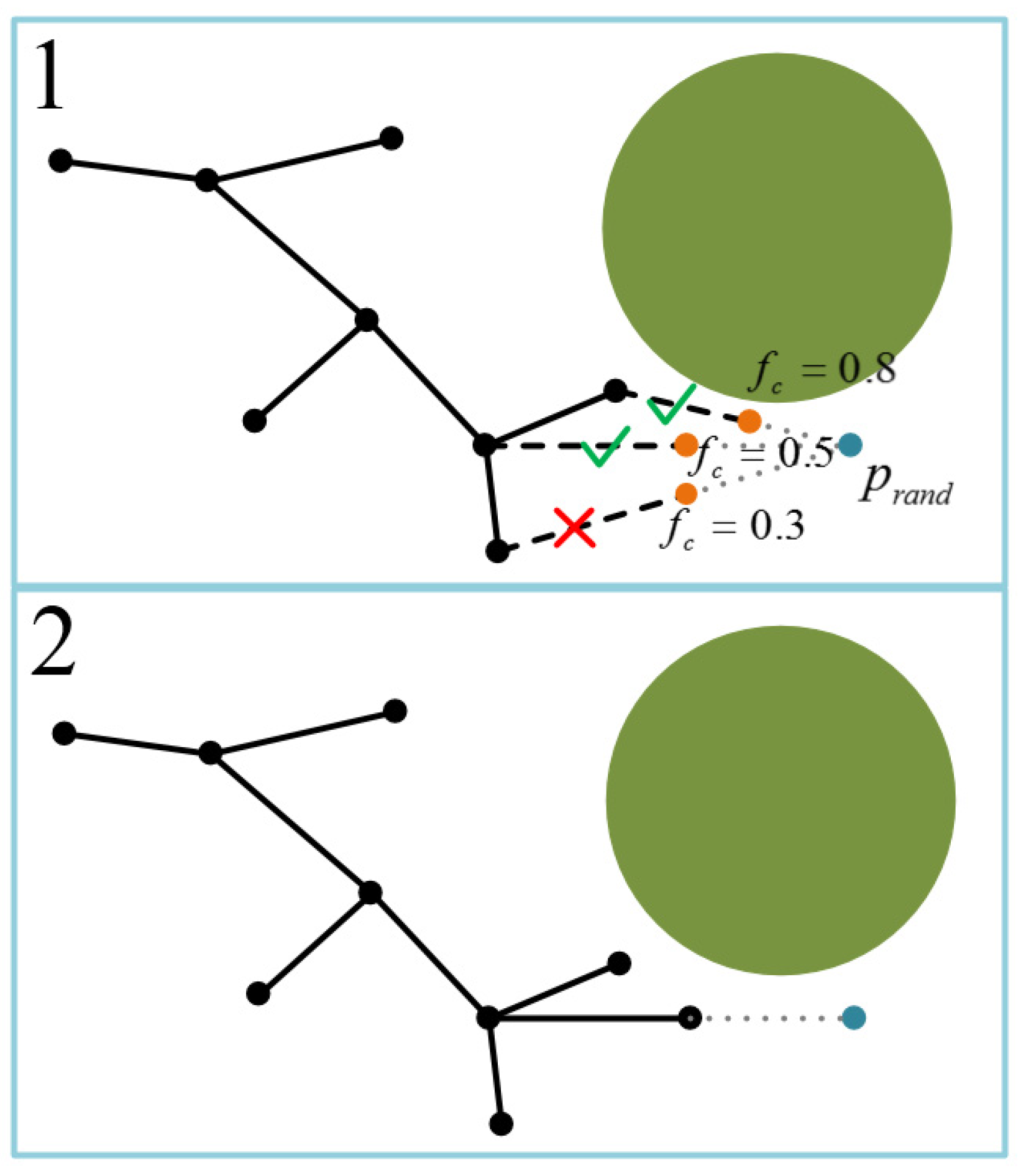
As shown in Figure 2, after obtaining the sample node $p_{rand}$, we use $\mathrm{Heuristic}\_\cos \mathrm{t}( )$ to return the new node $p_{new}$. The heuristic information process for guiding new node expansion is shown in Algorithm 2. First, the Euclidean distances between each tree node $p_v$ and $p_{rand}$ are calculated separately. If the distance between tree nodes $p_v$ and $p_{rand}$ is less than the maximum extended distance given by FC-RRT*, and is greater than the shortest path segment constraint distance $l_{\min }$, then $p_{rand}$ is determined as a potential new node. If this distance is greater than $l_{\min }$, then the vertex generated by extending the length $\delta$ along the tree node $p_v$ in the direction of $p_v$ to $p_{rand}$ is calculated as a potential new node.

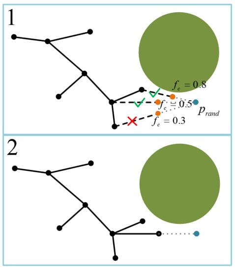
Figure 2. No. 1 shows the flight constraint determination (true or false symbol) and the flight cost f_c for potential new nodes (orange nodes). No. 2 shows that the new node expansion of FC-RRT* has been completed. The black nodes and edges are the trees that have been generated, and the blue node is p_rand.

Algorithm 2:$\mathrm{Heuristic}\_\cos \mathrm{t}(T.V,p_{rand})$

$\begin{array}{l}1: \mathbf{for} all p_v\in T.V \mathbf{do}\\ 2:\hspace{1em} \mathbf{if}(l_{\min }\le \parallel p_v-p_{rand}\parallel \le \delta )\\ 3:\hspace{1em}\hspace{1em} p_{new}\leftarrow p_{rand}\\ 4:\hspace{1em} \mathbf{elseif}(\parallel p_v-p_{rand}\parallel >\delta )\\ 5:\hspace{1em}\hspace{1em}\hspace{1em} p_{new}\leftarrow p_v+\delta \frac{p_{rand}-p_v}{\parallel p_{rand}-p_v\parallel }\\ 6:\hspace{1em} \mathbf{if}(\mathrm{collision}\_\mathrm{free}(p_v,p_{new})\wedge \\ \hspace{1em}\hspace{1em}\hspace{1em}\mathrm{UAV}\_\mathrm{free}(p_v,p_{new}))\mathbf{then}\\ 6:\hspace{1em}\hspace{1em}c\leftarrow {\lambda }_l{f}_l( p_v,p_{rand})+{\lambda }_t{f}_t( p_v,p_{new})\\ 7:\hspace{1em} \mathbf{else}\\ 8:\hspace{1em}\hspace{0.17em} \mathbf{continue}\\ 9: p_{new}\leftarrow \mathrm{argmin}(c)\end{array}$

Then, environmental constraints and flight constraints are detected for the potential edge $(p_v,p_{new})$. We use $\mathrm{collision}\_\mathrm{free}( )$ to detect collisions with threats and terrain. Additionally, we use $\mathrm{UAV}\_\mathrm{free}( )$ to detect whether the planned path satisfies the turning angle and climbing/gliding angle constraints.

If both constraints are satisfied, then the designed flight cost function is used to calculate the cost between the potential new node and each tree node $p_v$. The Euclidean distance between the sample node $p_{rand}$ and each tree node $p_v$ is calculated directly to determine the path length cost $f_l$. However, for the calculation of the threat strength cost $f_t$, due to the limitation of the maximum extension length $\delta$, the new node is only determined within the range of $\delta$ around the tree node. Therefore, in order to evaluate the threat strength correctly, we choose the edge consisting of $p_v$ and each potential new node to calculate the threat strength cost. After calculating the flight cost between each tree node $p_v$ and $p_{rand}$, the potential new node with the minimum flight cost is selected as the new node $p_{new}$ by $\mathrm{argmin}( )$.

3.4. Parent Node Updating Based on Flight Cost

In Section 3.2, we use heuristic information including threat strength and path length cost to guide the new node expansion, so that FC-RRT* meets the path length and safety requirements of UAV path planning as soon as the new node is determined. In order to further guide path generation, the evaluation approach of using Euclidean distance as the updating parent node in standard RRT* should also be improved. Therefore, we introduce the flight cost function to the optimal parent node updating in FC-RRT* in order to plan an optimal path that can be evaluated simultaneously with threat strength and path length.

To determine the neighbor region range, the tree nodes were selected from the ball with the radius setting ${\gamma }_3{\left(\log i/i\right)}^{1/3}$ (where ${\gamma }_3>2^n(1+1/n)\mu [C_{free}]$) [42].

The parent node updating approach in the FC-RRT* neighborhood is shown in Algorithm 3, and the following analysis takes the first call of $\mathrm{rewire}\_\mathrm{ImpRRT}*( )$ as an example. The standard RRT* first detects whether the edge $(p_{new},p_{near})$ is collision-free, and if true, the parent node is updated according to the Euclidean measure [21]. However, for the UAV, measuring the path by distance alone cannot ensure path safety. Additionally, the neighbor region node $p_{near}$ with the lowest path length cost may not satisfy the turning angle constraint or the climbing/gliding angle constraint. Moreover, there is a maximum path length constraint for the UAV. If the planned path length exceeds the maximum range limit, then the UAV cannot complete the mission.

Algorithm 3:$\mathrm{rewire}\_\mathrm{ImpRRT}*(x_1,x_2)$

$\begin{array}{l}1: \mathbf{if}(\mathrm{collision}\_\mathrm{free}(x_1,x_2)\wedge \\ \mathrm{UAV}\_\mathrm{free}(x_1,x_2))\mathbf{then}\\ 2: c\leftarrow f_c(x_1,x_2)\\ 3: \mathbf{if}(f_{c,T}(x_1)+c<f_{c,T}(x_2)\wedge \\ \mathrm{lenth}\_\max (x_1,x_2))\le L_{\max }\mathbf{then}\\ 4: T.\mathrm{parent}(x_2)\leftarrow x_1\end{array}$

Therefore, the edge connecting the potential parent node and the new node is detected to determine whether it meets the performance constraints or not (through $\mathrm{UAV}\_\mathrm{free}( )$), and whether the edge is collision-free in the flight environment (through $\mathrm{collision}\_\mathrm{free}( )$). Then, we evaluated the optimal parent node updating by introducing the flight cost function in order to guarantee that the UAV is kept away from the threat while also obtaining the shortest path. The flight cost from the start node $p_{start}$ through each $p_{near}$ to $p_{new}$ is calculated separately. Additionally, after that, the $p_{near}$ with the lowest cost is selected as the parent node. Finally, $\mathrm{lenth}\_\max ( )$ is used to determine whether the maximum path length constraint is satisfied. The $\mathrm{lenth}\_\max ( )$ is calculated as

$$\mathrm{lenth}\_\max (x_1,x_2)=f_l(p_{start},x_1)+f_l(x_1,x_2)+\left|\right|p_{goal}-x_2\left|\right|$$

(15)

4. Analysis

In this section, the FC-RRT* algorithm is theoretically analyzed in combination with RRT* [32]. Through analysis, we prove that the proposed FC-RRT* has probabilistic completeness and asymptotic optimality. Meanwhile, the asymptotic computational complexity is basically the same as that of RRT*.

4.1. Probabilistic Completeness

This section analyzes the probabilistic completeness of FC-RRT*. Most sampling-based path planning algorithms are probabilistically complete, and the definition of probabilistic completeness is shown below.

Definition 3 (Probabilistic completeness).

Given the starting node and the set of desired goal nodes, if for any robust feasible path planning problem, the following equation is satisfied, i.e.,

$$\underset{n\to \infty }{\lim \inf } \mathbb{P}\left({\sigma }_{n,ALG}\cap P_{goal}\ne \varnothing \right)=1,$$

(16)

algorithm $ALG$ is considered to be probability complete.

Referring to the description of probability completeness in Definition 3, the probability completeness of FC-RRT* is described in Theorem 1.

Theorem 1 (Probabilistic completeness of FC-RRT*).

When the number of given samples is infinite, the probability of FC-RRT* finding a feasible solution for any robust feasible path planning problem is one, that is,

$$\underset{n\to \infty }{\lim \inf }\mathbb{P}\left({\sigma }_{n,FC-RRT*}\in C_{free},{\sigma }_{n,FC-RRT*}(0)=p_{start},{\sigma }_{n,FC-RRT*}(1)\in P_{goal}\right)=1$$

(17)

Proof of Theorem 1.

The proof of Theorem 1 is based on the following three arguments:

• The random tree generated by FC-RRT* must include $p_{start}$ as one of its vertices. Meanwhile, the target node must be within the set of desired goal nodes $P_{goal}$, i.e., ${\sigma }_{n,FC-RRT*}(0)=p_{start},{\sigma }_{n,FC-RRT*}(1)\in P_{goal}$, which is the same as RRT*.
• Similar to RRT *, the FC-RRT* planning tree is connected (see Algorithm 1). In other words, any random sample can be connected to the nearest vertex in the neighbor of the tree.
• FC-RRT* sets the target node in the set of desired goal nodes. Therefore, when the random sampling is infinite, the probability of generating FC-RRT* random tree to the target region is close to one. □

Based on the above three arguments, we are able to prove that when any path planning problem is given, FC-RRT* can find a feasible path and approach a probability of 1 as the number of samples approaches infinity (the premise of this conclusion is that there is a feasible solution to a given path planning problem). Therefore, FC-RRT* and RRT* also guarantee probability completeness.

4.2. Asymptotic Optimality

FC-RRT* inherits the asymptotic optimality of standard RRT *. This section analyzes the asymptotic optimality of FC-RRT* in dealing with path planning problems. Firstly, the definition of asymptotic optimality is given as follows.

Definition 4 (Asymptotic optimality).

For any path planning problem, when the number of samples approaches infinity, the algorithm $ALG$is said to be asymptotically optimal if it can return the tree graph of the least cost solution. Similar to RRT*, we set the following assumptions to prove that FC-RRT* is asymptotically optimal. They have been used to prove that RRT * is asymptotically optimal [32].

Assumption 1 (Additivity of the cost).

For any two collision free paths, i.e., ${\sigma }_1,{\sigma }_2\in C_{free}$, the cost function $f_c(·)$ must satisfy$f_c\left({\sigma }_1\right)\le f_c\left({\sigma }_1|{\sigma }_2\right):f_c\left({\sigma }_1\right)+f_c\left({\sigma }_2\right)$.

Assumption 2 (Continuity of the cost).

The cost function$f_c(·)$is a Lipschitz continuous function, and there is a constant $\delta$ such that any two very close collision free paths${\sigma }_1:\left[0,g_1\right],{\sigma }_2:\left[0,g_2\right]\in C_{free}$, have $|f_c\left({\sigma }_1\right)-f_c\left({\sigma }_2\right)|\le \delta \underset{\tau :\left[0,1\right]}{\sup }\Vert {\sigma }_1\left(\tau g_1\right)-{\sigma }_2\left(\tau g_2\right)\Vert$.

Assumption 3 (

$\gamma$-spacing of the obstacle). For any sampling node $p$, there is a ball region in collision free space C with a radius of $\gamma \in {ℝ}_{>0}$ and center of another node $p_1\in C_{free}$, i.e., $p\in {\mathfrak{B}}_{P_1,\gamma }$.

Based on the above assumptions, the asymptotic optimality description of FC-RRT* is given as follows:

Theorem 2 (Asymptotic optimality of FC-RRT*).

Let Assumptions 1, 2 and 3 hold; when the number of samples is infinite, the probability of FC-RRT* gradually converging to the optimal solution of the given path planning problem is

$$\mathbb{P}\left(\underset{n\to \infty }{\lim \sup } \left(c\left({\sigma }_{n,FC-RRT*}\right)=c^{*}\right)\right)=1,$$

(18)

where $c^{*}$ is the optimal solution of the path planning problem.

Proof of Theorem 2.

Assumption 1 indicates that the cost function of the algorithm needs to be additive, and the cost cannot be negative. When the algorithm runs rewiring processes, different path segments need to be added for comparison (see $\mathrm{rewire}\_\mathrm{ImpRRT}*( )$). The standard RRT * takes the Euclidean distance as the cost, which must satisfy Assumption 1 (i.e., $f_c\left({\sigma }_1\right)=f_l\left({\sigma }_1\right)$). The cost function $f_c(·)$ of FC-RRT* consists of the path length cost $f_l(·)$ and path threat cost $f_t(·)$, and $f_t(·)\ge 0$. For any weight combination $\left[{\lambda }_1,{\lambda }_2\right]$ (${\lambda }_1+{\lambda }_2=1$),

$$f_c\left({\sigma }_1\right):f_l\left({\sigma }_1\right)+f_t\left({\sigma }_1\right)\le f_l\left({\sigma }_1\right)+f_t\left({\sigma }_1\right)+f_l\left({\sigma }_2\right)+f_t\left({\sigma }_2\right)$$

(19)

Therefore, FC-RRT* also satisfies Assumption 1. □

Assumption 2 indicates that two very close paths have similar costs. Similar to RRT*, FC-RRT* also holds for this assumption. For two very close paths, the path lengths are similar. Moreover, because the distance between the two close paths and the threat is very similar, the path threat cost is also similar.

Assumption 3 indicates that there is a collision free region around the feasible path. The algorithm can select the sampling node with the lowest cost from the sampling nodes in the region in order to converge the algorithm to the optimal path. The determination of the neighborhood radius $\gamma$ using the FC-RRT* algorithm is the same as RRT*, i.e., ${\gamma }_3\ge {\gamma }_3^{*}$. This ensures that at least one node of the tree $\tau =(\upsilon ,\epsilon )$ falls into this region when a large number of samples are taken. This means that when calling the $\mathrm{rewire}\_\mathrm{ImpRRT}*( )$ function to select the parent node, the node with a lesser cost is likely to be rewired to optimize the path. Therefore, when the sampling times approach infinity, the probability that the path cost variation $\Vert f_c\left({\sigma }_1\right)-f_c\left({\sigma }_1\right)\Vert$ of the two feasible paths is approximately zero is one. Therefore, FC-RRT* is proven to be asymptotically optimal.

4.3. Computational Complexity

In this section, we mainly compare the asymptotical computational complexity of standard RRT* and FC-RRT*. The comparative analysis shows that the asymptotic computational complexity of the two algorithms is almost the same.

In order to compare the progressive computational complexity of RRT* and FC-RRT*, we need to evaluate the time required by comparing the number of execution steps of each process. Note that the $\mathrm{Sample}(·)$, $\mathrm{collision}\_\mathrm{free}(·)$ and $\mathrm{Near}(·)$ processes of the two algorithms are the same, and they can be performed in a certain number of steps (i.e., the execution of these procedures is independent of the number of vertices in the tree.). For each iteration $i$, $\mathrm{Sample}(·)$ executes at least once, $\mathrm{collision}\_\mathrm{free}(·)$ executes at least three times, and $\mathrm{Near}(·)$ executes at least once. The difference is that the standard RRT* divides the new node expansion into two processes (e.g., the authors of [32] called them the $\mathrm{Nearest}(·)$ and $\mathrm{steer}(·)$ processes), and the proposed FC-RRT* algorithm directly returns to the new node through the $\mathrm{Heuristic}\_\cos \mathrm{t}(·)$ process. Therefore, the asymptotic computational complexity of the $\mathrm{Heuristic}\_\cos \mathrm{t}(·)$ process needs to be considered.

The $\mathrm{steer}(·)$ process of RRT* is only a simple expansion of nodes, and it basically does not affect the calculation time. However, both the $\mathrm{Heuristic}\_\cos \mathrm{t}(·)$ and $\mathrm{Nearest}(·)$ processes involve the problem of finding the nearest neighbor. The study conducted in [43] shows that the nearest neighbor search takes at least logarithmic time, and each iteration changes according to the changes that take place in the sampling points (i.e., process execution is related to the number of vertices of the tree). For FC-RRT* and RRT*, because each iteration has only one sampling, their nodes in iteration $i$ are the same, i.e., ${\mathcal{V}}_i^{RRT*}={\mathcal{V}}_i^{FC-RRT*}$. Therefore, both RRT* and FC-RRT* need at least logarithmic time $\log \left(n\right)$ to find the nearest neighbor in iteration $i$. Therefore, FC-RRT* and RRT* have almost the same asymptotic computational complexity.

Theorem 3.

There is a constant A such that,

$$\underset{n\to \infty }{\lim }\mathbb{E}\left[\frac{{\mathcal{S}}_i^{RRT*}}{{\mathcal{S}}_i^{FC-RRT*}}\right]\le \alpha ,$$

(20)

where ${\mathcal{S}}_i^{RRT*}$ and ${\mathcal{S}}_i^{FC-RRT*}$ represent the numbers of steps involved in RRT* and FC-RRT*, respectively, in the iteration.

5. Simulation and Analysis

In order to comprehensively evaluate the effectiveness of the proposed FC-RRT* algorithm, we carried out simulation evaluation and analysis.

There is no widely accepted environmental standard model in UAV path planning. For sampling-based path planning methods, we usually adopt basic configurations to represent obstacles or threats in the scene. Therefore, in this paper, when establishing the threat model, as in [44], a hemispherical model to approximately describe the warning radar and its threat area is implemented, and the model uses the cylindrical model to approximately describe the anti-aircraft gun building and its attack range. The cone model was used to approximately describe the tower (since the tower has no detection or strike capability, it is treated as a no-fly zone). However, the use of a basic configuration results in a lot of information regarding the terrain being lost. Therefore, in this paper, a real elevation map was constructed to represent the terrain in order to truly reflect the terrain threat information.

Table 1 shows some basic FC-RRT* parameters, where Case 1, Case 2, and Case 3 are different weight assignments in the flight cost function, respectively. Additionally, the established parameters for radar, anti-aircraft gun, and tower are indicated.

Table 1. Parameter values.

Parameter	Value
Case 1	${\lambda }_l$$=0.1; {\lambda }_t$ = 0.9
Case 2	${\lambda }_l$$=0.5; {\lambda }_t$ = 0.5
Case 3	${\lambda }_l$$=0.9; {\lambda }_t$ = 0.1
$L_{th}$	20 m
$\delta$	70 m
$N_0$	15
${\varphi }_{\max }$	45°
${\gamma }_{\max }$	30°
$l_{\min }$	30 m
Iter	2000
Start	(40,40,30)
Target	(350,350,50)
Rader	Center	radius
	(100,80,0)	35
	(100,350,5)	35
	(170,230,20)	35
	(280,200,20)	35
Anti-air. gun	Center	radius	height
	(70,170,0)	30	40
	(170,140,0)	30	40
	(300,100,0)	30	40
	(260,180,0)	25	40
Control tower	Center	radius	height
	(200,290,10)	15	50
	(100,275,10)	20	40

5.1. Simulation and Analysis of FC-RRT* in the Complex Environment

Through the complex flight environment, FC-RRT* is simulated and analyzed verifying the effectiveness and superiority of the heuristic information to guide new node expansion and parent node updating.

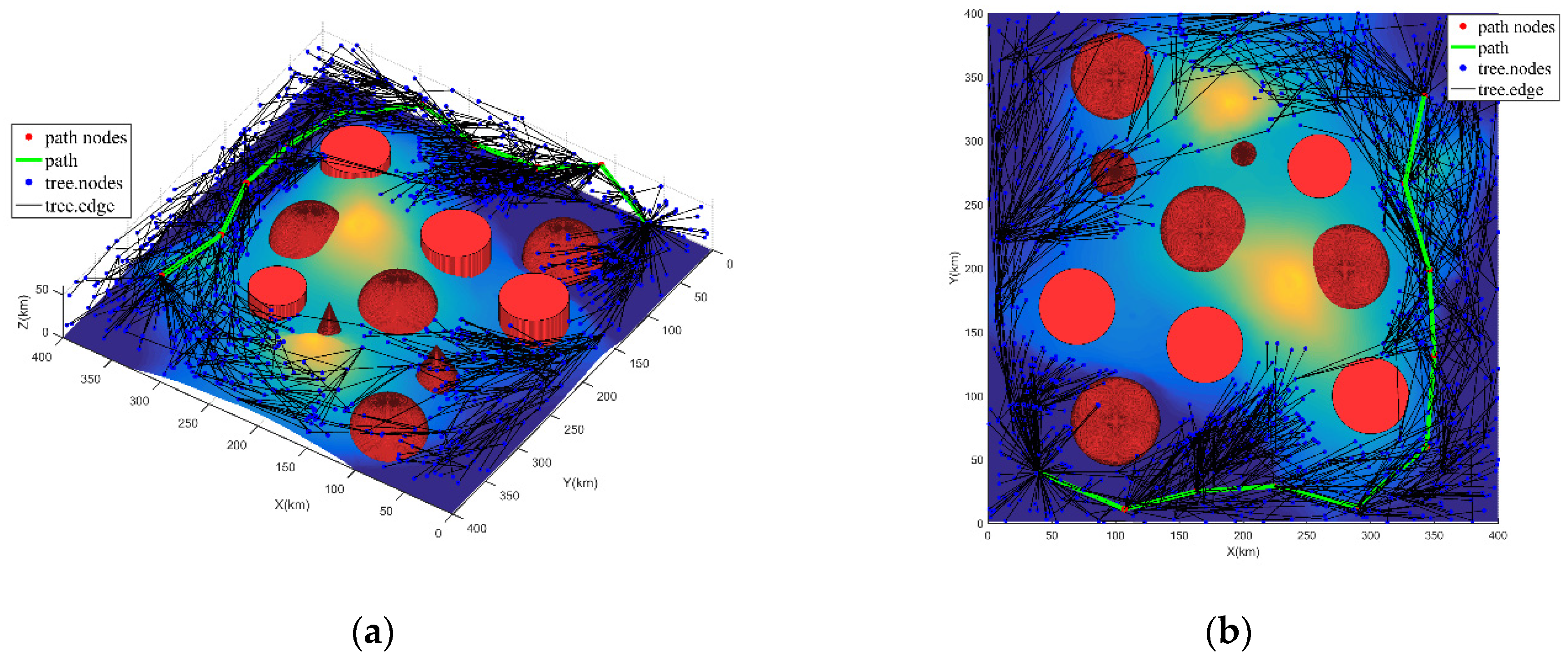
Figure 3, Figure 4 and Figure 5 show the directed tree graph and planning path of FC-RRT* in three different cases. Table 2 shows the statistical results, including the number of tree nodes, the number of tree nodes in threat range $L_{th}$, the path length, the minimal distance between the path and the threats, the threat value of the path, the proportion of the threat impact path length in the total path length, and the success rate of 50 experiments.

Figure 3. Directed tree graph and path of UAV in Case 1, i.e., ${\lambda }_l$ =0.1 and ${\lambda }_t$ = 0.9: (a) 3D view of Case 1; (b) 2D top view of Case 1.

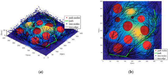
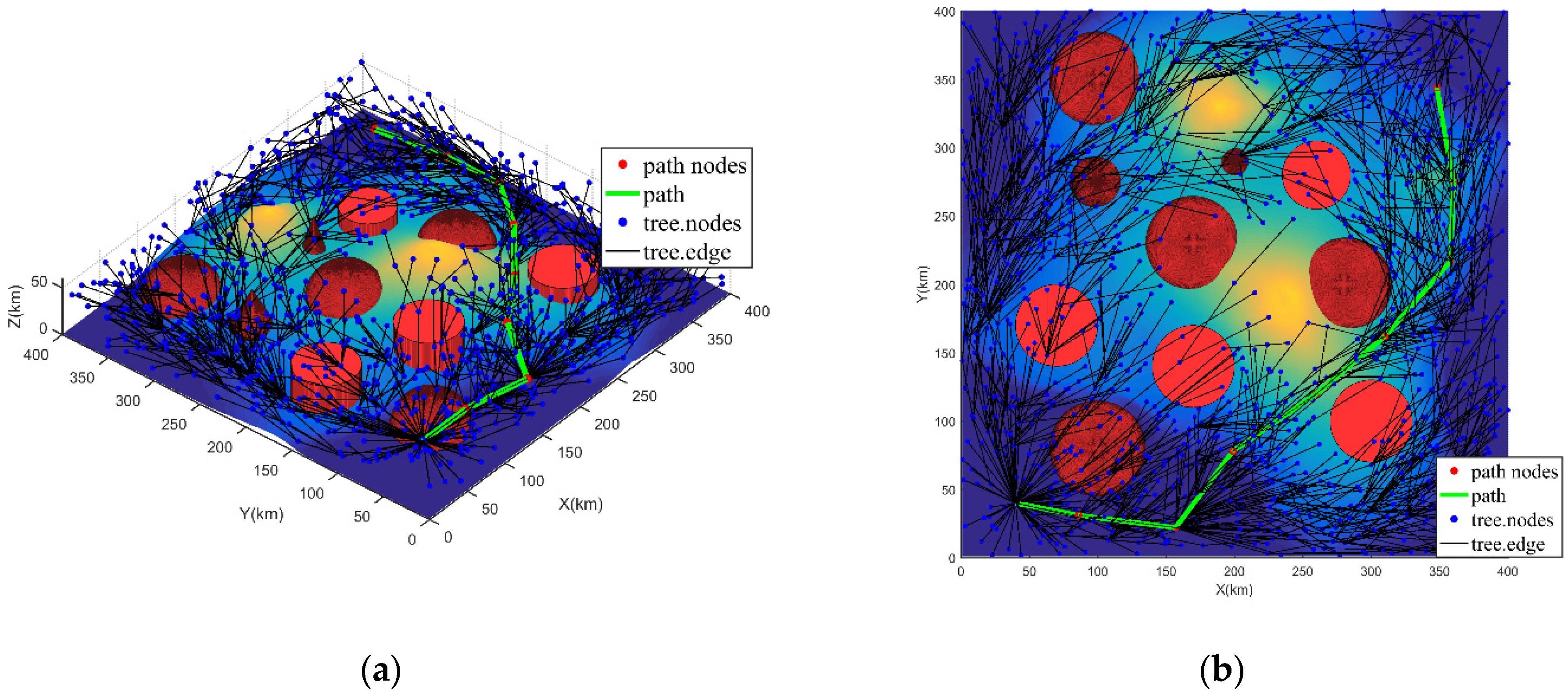
Figure 4. Directed tree graph and path of UAV in Case 2, i.e., ${\lambda }_l$ = 0.5 and ${\lambda }_t$ = 0.5: (a) 3D view of Case 2; (b) 2D top view of Case 2.

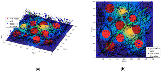
Figure 5. Directed tree graph and path of UAV in Case 3, i.e., ${\lambda }_l$ = 0.9 and ${\lambda }_t$ = 0.1: (a) 3D view of Case 3; (b) 2D top view of Case 3.

Table 2. Statistical results of the FC-RRT* for three different weights.

Cases	$\mathbf{Case}1 ({\mathit{\lambda }}_{\mathit{l}}$$= 0.1 \mathbf{and} {\mathit{\lambda }}_{\mathit{t}} = 0.9)$	$\mathbf{Case}2 ({\mathit{\lambda }}_{\mathit{l}}$$= 0.5 \mathbf{and} {\mathit{\lambda }}_{\mathit{t}} = 0.5)$	$\mathbf{Case}3 ({\mathit{\lambda }}_{\mathit{l}}$$= 0.1 \mathbf{and} {\mathit{\lambda }}_{\mathit{t}} = 0.9)$
Tree nodes	1426	1435	1412
$\mathrm{Tree} \mathrm{nodes} \mathrm{in}{L}_{th}$	58	456	871
Path Length (m)	617.7	532.2	479.2
minDis. to Thr. (m)	18.71	12.62	4.90
Thr. cost	8.29	37.58	95.833
Path in Thr.(%)	2.65	44.19	81.78
Succ.Rate (%)	94	92	94

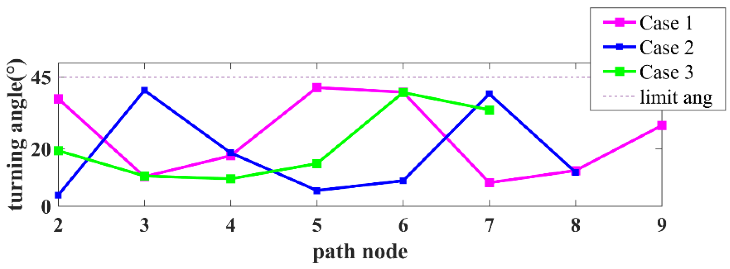
From the simulation success rate in Table 2, after improving the new node determination and parent node update, and introducing the UAV constraint, FC-RRT* still managed successful path planning in the complex environment. From Figure 6 and Figure 7, the path planned using FC-RRT* satisfies the turning angle and climbing/gliding angle constraints, and the turning and climbing/gliding angles are relatively smooth.

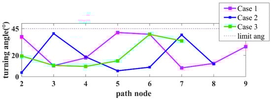
Figure 6. Turning angle of path nodes in three different cases.

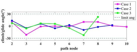
Figure 7. Climbing/gliding angle of path nodes in three different cases.

Furthermore, since the flight cost function is applied as heuristic information to guide the new node expansion, from Figure 3, Figure 4 and Figure 5, the distribution of the tree nodes differs significantly based on the three weights. Case 1 represents a weight assignment that focuses on path safety with little consideration of path length cost. Hence, the tree nodes in Figure 3 are not expanded near the threats. Most of them are mostly concentrated within a certain distance from the threat. Additionally, from Table 2, the number of nodes in the threat range $L_{th}$ for Case 1 shows that only a few tree nodes are located within the threat scope. Case 2 represents the weight assignment for both the path safety and path length requirements, so a certain number of tree nodes exist in the threat impact range, which is shown in Figure 4. Meanwhile, as shown in Table 2, the number of tree nodes in the threat range $L_{th}$ of Case 2 has increased compared to Case 1. The weight assignment of Case 3 represents the desire to achieve close to the lowest path loss, even though it sacrifices path safety. Therefore, from Figure 5, the tree nodes are basically evenly distributed in the sampling environment. Additionally, the number of nodes in the threat range $L_{th}$ in Table 2 is also the highest. From the above, the weights ${\lambda }_l$ and ${\lambda }_t$ in the flight cost function affect the expansion of new nodes. Namely, using the flight cost function as heuristic information can effectively guide the expansion of new nodes, thus guiding the path planning from the front-end.

Combined with Figure 3, Figure 4 and Figure 5 and Table 2, the planning paths under three different weight distributions are quite different. From Figure 3, the planning path in Case 1 has a larger distance between the path and the threat, which also results in a longer path length. Meanwhile, comparing the statistical results of the three cases in Table 2, it can be seen that Case1 has the largest distance between the path and the threat; the threat strength value and the percentage of threat paths are the lowest; and the path length is the longest. This confirms that at the weight of Case1, the planning path focuses on path safety, although the path length cost is more expensive. From Figure 4 for Case 2, the distance between the planned path and threat and the path length cost are both at the medium level (compare with other cases). Additionally, from Table 2, the statistical results of Case 2 are moderate in the three cases. This proves that path safety has a similar importance to path length at the weight of Case 2. As seen in Figure 5 for Case 3, the path length is the shortest, but the distance between the path and the threat is the shortest. This is also reflected in the comparison of the statistical results in Table 2, where the path length is the shortest of the three weights. However, the distance between path and threats is the smallest, and the threat path value and the threat path percentage are largest. Hence, although the weight of Case 3 plans the shortest path, it greatly affects path safety and reduces the probability of survival. From the above, the flight cost function can effectively guide the path planning of the UAV and obtain the optimal path required by the user.

In summary, the simulation results show that FC-RRT* is suitable for UAV path planning in the complex environment, and that it meets the path safety and path length requirements. In terms of front-end new node expansion and back-end parent node updating, the flight cost function and flight constraint are introduced twice, meaning that FC-RRT* plans an optimal path with the shortest length while satisfying the path safety requirements. Additionally, the weight assignment of different flight cost functions in the algorithm can guide the generation of paths with different requirements. Case 1 indicates that the path with the highest survival probability is preferred, while there is essentially no requirement for path length cost. Therefore, it can be used for military missions such as cruising and long-range surveillance on the battlefield. Case 2 indicates that both path safety and path length are more important. It can be used for military missions for applications such as enemy suppression and for striking enemy facilities. The application of Case 3 allows the UAV to quickly pass through enemy threats while ignoring the probability of survival and the ability to avoid threats, so it can be applied to speed escape and surprise defense situations.

5.2. Comparison and Discussion

In order to further verify the superiority of the FC-RRT*, we compared it to the standard RRT*. In this experiment, the flight environment is adjusted to clearly show the comparison of the algorithms. The adjusted parameters are shown in Table 3, and other parameters are shown in Table 1.

Table 3. Parameters that were adjusted in the comparison.

Parameter	Value
Wig	${\lambda }_l$$=0.6; {\lambda }_t$ = 0.4
Rader	Center	radius
	(100,80,0)	40
	(100,350,5)	40
	(170,230,20)	40
	(280,200,20)	40
Anti-air. gun	Center	radius	height
	(70,170,0)	30	50
	(170,140,0)	30	50
	(300,100,0)	30	50
	(260,180,0)	25	50
Control tower	Center	radius	height
	(200,290,10)	15	50
	(100,275,10)	20	40

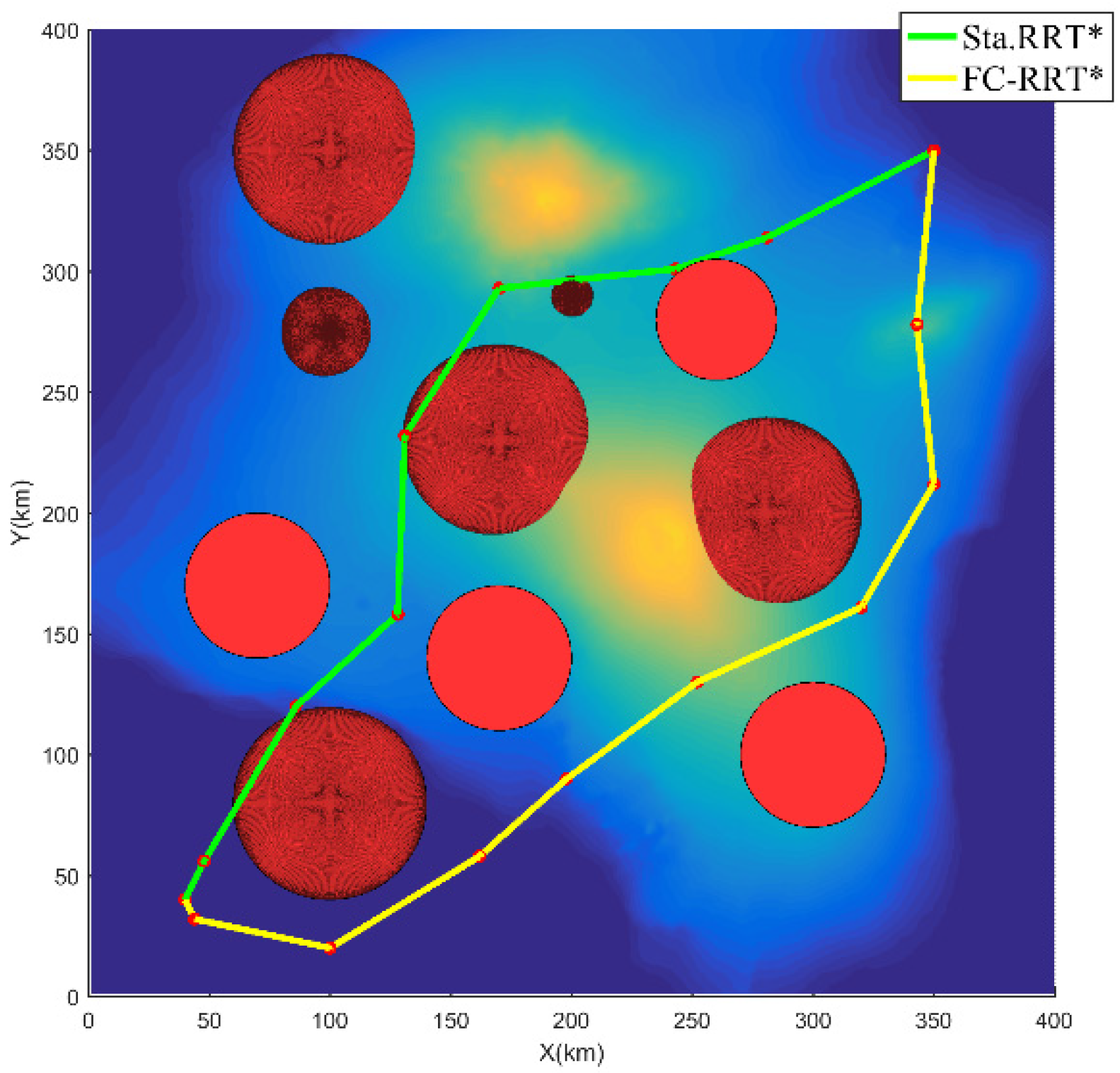
From the tree node distribution in Figure 8, since RRT* only considers the Euclidean distance when new nodes are expanded, the tree nodes generated by the algorithm are evenly distributed in the sampling space. However, the FC-RRT* algorithm adopts the proposed flight cost function to inspire guiding new node expansion, so the number of tree nodes near the threat region is significantly smaller (refer to Figure 3). Additionally, this is demonstrated by the comparison of the number of tree nodes in the threat range $L_{th}$ in Table 4. Meanwhile, from Table 4, the length of the RRT* planning path is shorter compared to FC-RRT*. However, compared to FC-RRT*, the path planned by RRT* has a larger threat value and the smaller nearest distance to the threat, and most of the path is in the affected range of threat. However, considering the path safety of the UAV in the complex environment created for these simulations, the path planned by FC-RRT* adopts the flight cost function to guide the expansion of new nodes and to direct parent node updating. Although this approach results in a longer path, both the path threat value and the percentage of the path affected by threats are smaller than RRT*, and the closest distance to the threat is relatively large. Therefore, the RRT* path is too close to the threat, which affects path safety. In contrast, in FC-RRT*, the planning path is far away from the threat, which guarantees path safety while maintaining the shortest flight path.

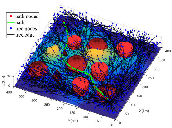
Figure 8. Directed tree graph and path of RRT*.

Table 4. Statistical results comparison between FC-RRT* and RRT*.

Algorithms	Sta. RRT*	FC-RRT*
Tree nodes	1460	1446
$\mathrm{Tree} \mathrm{nodes} \mathrm{in}{L}_{th}$	1049	414
Path Length (m)	482.06	534.88
minDis. to Thr. (m)	0.41	10.54
Thr. cost	286.44	11.99
Path in Thr.(%)	95.34	56.62
Succ. Rate (%)	96	98

Additionally, from Figure 9 and Figure 10, the path planned by RRT* is shorter but has more large-angle turns, while FC-RRT* generates a path with fewer turns and the path is smoother. Further, from Figure 11 and Figure 12, some of the turning and climbing/gliding angles of the path points do not satisfy the UAV constraint in standard RRT*. However, for FC-RRT*, the planned path satisfies the angle constraints and is relatively smooth.

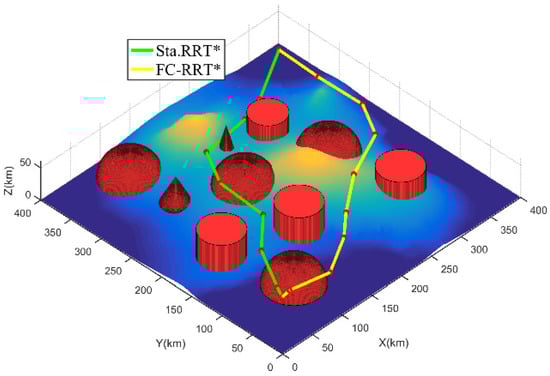
Figure 9. Path comparison of RRT* and FC-RRT* in 3D view.

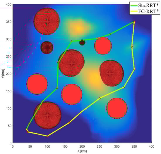
Figure 10. The 2D image of Figure 9.

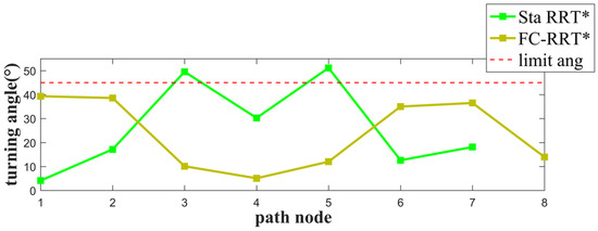
Figure 11. The turning angle comparison between FC-RRT* and RRT*.

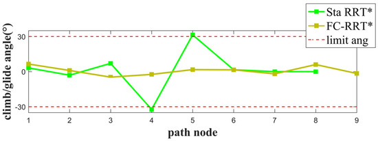
Figure 12. The climbing/gliding angle comparison between FC-RRT* and RRT*.

In summary, comparing the RRT* and FC-RRT* performance for UAV path planning in the complex environment, the path planned by RRT* is close to the threat, meaning that path safety is not guaranteed. Additionally, there are too many large angle-turns and cannot meet the flight constraints. Hence, RRT* is not suitable for UAV path planning. However, for FC-RRT*, both the path threat strength and path length cost are considered, and the flight cost function is designed to guide the new node to expand so that the new node can expand to the environment that meets the path safety requirements. However, for FC-RRT*, the new node is extended to the path safety environment because of the application of the flight cost function that includes the threat strength and path length cost. Additionally, the flight cost function is used to guide optimal parent node updating. Therefore, the path planned by FC-RRT* is relatively far from the threats, guaranteeing path safety. At the same time, due to the introduction of the flight constraints in FC-RRT*, the path satisfies the constraints and the path is smoother compared with the standard RRT*. The experiment proves that FC-RRT* is suitable for UAV path planning in a complex environment and can meet the requirements of military operations.

5.3. Discussion before Actual Flight Test Preparation

Our paper mainly studies a three-dimensional path planning method that is suitable for UAVs. Considering the complexity of the battlefield environment and the diversity of obstacle threats, we proposed an FC-RRT* algorithm to meet the UAV planning requirements in this environment. In order to create the algorithm, we studied certain practical application values, and we have extended the discussion on the practical application of the algorithm in this section.

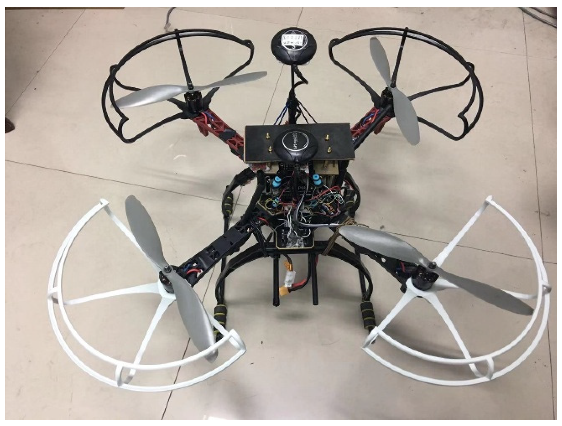
We selected the four-rotor UAVs that we designed in the laboratory to measure and record the relevant parameters and compared the obtained data with the simulation results of the algorithm in this paper in order to observe whether the simulation results in this paper can meet the parameter constraints of the UAV. In future flight tests in real-life conditions, we will select the same UAVS. The four-rotor UAV is shown in Figure 13, and the relevant UAV parameters are shown in Table 5. In order to fully introduce the four-rotor platform that we will use to conduct flight tests in the future, the relevant parameters of the self-designed autopilot are introduced in Table A1 in Appendix A.

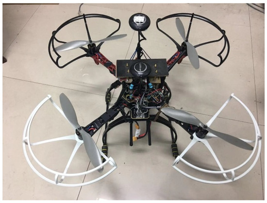
Figure 13. The self-designed four-rotor platform.

Table 5. The UAV specifications.

UAV	Specification
Take-off Weight	1 kg
Max Playload	0.5 kg
Wingspan	455 mm
Battery Capacity	5000 mAh
Max Forward Speed	4 m/s
Flight Time	28 min
Max Turning Angle	275°
Max Tilt Angle	45°

It can be seen from Table A1 that when a battery with a load capacity of 5000 mAh flies, the maximum flight time of the UAV is 28 min, and the maximum flight speed of the UAV is 4 m/s. Combined with the maximum planned UAV path length given in Table 2 and Table 4 in Section 5 of this article, it can be seen that the simulation results can meet the parameter conditions of the actual UAV flight length and can complete the flight in one full power load. At the same time, the maximum steering angle constraint and max-imum climb angle constraint of the UAV set in the simulation meet the angle constraint limit of the four-rotor UAV. Therefore, we can preliminarily determine that the algorithm developed in this paper can complete flight tests using the four-rotor UAV platform. Of course, this is only a preliminary judgment before the actual flight experiment. For some actual parameters, such as the influence of specific weather and wind direction, accurate data can be obtained during actual test flights in the future.

6. Conclusions

In this paper, we propose a path planning algorithm for UAVs in complex environments called FC-RRT*, which comprehensively considers the length of the path and the safety of the path to guarantee that a UAV is able to safely complete military missions. FC-RRT* improves and optimizes standard RRT*. First, we designed a flight cost function that includes both path threat strength and path length cost. Then, an approach using the flight cost function as heuristic information to guide the expansion of new nodes is proposed at the front-end, which enables new nodes to be expanded to a sampling space with high path safety. After that, we considered both the same flight cost function and flight constraints in the parent node update at the back-end. The path planned by FC-RRT* has the shortest distance and highest safety because it guides both the front-end and back-end. Then, we analyzed the FC-RRT* in depth. Simulations and comparisons prove that FC-RRT* is suitable for UAV path planning in a complex environment. Additionally, FC-RRT* can be applied to different military missions, such as cruising or long-range surveillance, striking enemy facilities, and battlefield speed escape or surprise defense.

Of course, this algorithm is not the only way to deal with UAV path planning in complex environments. Intelligent algorithms such as the genetic algorithm are also capable of this, but intelligent algorithms usually comprise a great deal of complexity. Therefore, as an algorithm with relatively low computational complexity, the algorithm proposed in this paper improves the computational efficiency on the premise of obtaining similar results. Meanwhile, we hope to conduct more in-depth research on this algorithm in future research, including but not limited to the theoretical improvement and actual flight verification of the algorithm, so that our algorithm can have stronger application value. Additionally, FC-RRT* is only suitable for static UAV path planning, which means that all environmental information needs to be known. Therefore, further studies need to be conducted on dynamic path planning algorithms in other complex environments.

References

- Papadopoulou, E.-E.; Vasilakos, C.; Zouros, N.; Soulakellis, N. DEM-Based UAV Flight Planning for 3D Mapping of Geosites: The Case of Olympus Tectonic Window, Lesvos, Greece. ISPRS Int. J. Geo-Inf. 2021, 10, 535. [Google Scholar] [CrossRef]
- Patle, B.K.; Babu, L.G.; Pandey, A.; Parhi, D.R.K.; Jagadeesh, A. A review: On path planning strategies for navigation of mobile robot. Defin. Technol. 2019, 15, 582–606. [Google Scholar] [CrossRef]
- Fu, B.; Chen, L.; Zhou, Y.; Zheng, D.; Wei, Z.; Dai, J.; Pan, H. An improved A* algorithm for the industrial robot path planning with high success rate and short length. Robot. Auton. Syst. 2018, 106, 26–37. [Google Scholar] [CrossRef]
- Zhao, L.; Yan, L.; Hu, X.; Yuan, J.; Liu, Z. Efficient and High Path Quality Autonomous Exploration and Trajectory Planning of UAV in an Unknown Environment. ISPRS Int. J. Geo-Inf. 2021, 10, 631. [Google Scholar] [CrossRef]
- Phung, M.D.; Ha, Q.P. Safety-enhanced UAV path planning with spherical vector-based particle swarm optimization. Appl. Soft Comput. 2021, 107, 107376. [Google Scholar] [CrossRef]
- Liao, S.L.; Zhu, R.M.; Wu, N.Q.; Shaikh, T.A.; Sharaf, M.; Mostafa, A.M. Path planning for moving target tracking by fixed-wing UAV. Defin. Technol. 2020, 16, 811–824. [Google Scholar] [CrossRef]
- Wu, G.; Atilla, I.; Tahsin, T.; Terziev, M.; Wang, L.C. Long-voyage route planning method based on multi-scale visibility graph for autonomous ships. Ocean Eng. 2021, 219, 108242. [Google Scholar] [CrossRef]
- Chi, W.; Ding, Z.; Wang, J.; Chen, G.; Sun, L. A Generalized Voronoi Diagram based Efficient Heuristic Path Planning Method for RRTs in Mobile Robots. IEEE Trans. Ind. Electron. 2021, 65, 4926–4937. [Google Scholar] [CrossRef]
- Fink, W.; Baker, V.R.; Brooks, A.J.W.; Flammia, M.; Dohm, J.M.; Tarbell, M.A. Globally optimal rover traverse planning in 3D using Dijkstra’s algorithm for multi-objective deployment scenarios. Planet. Space Sci. 2019, 179, 104707. [Google Scholar] [CrossRef]
- Chen, X.; Zhao, M.; Yin, L. Dynamic Path Planning of the UAV Avoiding Static and Moving Obstacles. J. Intell. Robot. Syst. Theory Appl. 2020, 99, 909–931. [Google Scholar] [CrossRef]
- Majumder, S.; Prasad, M.S. Three dimensional D∗ algorithm for incremental path planning in uncooperative environment. In Proceedings of the 3rd International Conference on Signal Processing and Integrated Networks, SPIN, Noida, India, 11–12 February 2016; Volume 2016, pp. 431–435. [Google Scholar]
- Ye, B.; Tang, Q.; Yao, J.; Gao, W. Collision-free path planning and delivery sequence optimization in noncoplanar radiation therapy. IEEE Trans. Cybern. 2019, 49, 42–55. [Google Scholar] [CrossRef] [PubMed]
- Yuan, C.; Liu, G.; Zhang, W.; Pan, X. An efficient RRT cache method in dynamic environments for path planning. Rob. Auton. Syst. 2020, 131, 103595. [Google Scholar] [CrossRef]
- Wu, Y.; Wu, S.; Hu, X. Cooperative Path Planning of UAVs UGVs for a Persistent Surveillance Task in Urban Environments. IEEE Internet Things J. 2021, 8, 4906–4919. [Google Scholar] [CrossRef]
- Yang, H.; Qi, J.; Miao, Y.; Sun, H.; Li, J. A New Robot Navigation Algorithm Based on a Double-Layer Ant Algorithm and Trajectory Optimization. IEEE Trans. Ind. Electron. 2019, 66, 8557–8566. [Google Scholar] [CrossRef] [Green Version]
- Rasekhipour, Y.; Khajepour, A.; Chen, S.K.; Litkouhi, B. A Potential Field-Based Model Predictive Path-Planning Controller for Autonomous Road Vehicles. IEEE Trans. Intell. Transp. Syst. 2017, 18, 1255–1267. [Google Scholar] [CrossRef]
- Liu, X.; Zhang, D.; Zhang, T.; Zhang, J.; Wang, J. A new path plan method based on hybrid algorithm of reinforcement learning and particle swarm optimization. Eng. Comput. 2021; ahead-of-print. [Google Scholar] [CrossRef]
- Wu, J.; Wang, H.; Zhang, M.; Yu, Y. On obstacle avoidance path planning in unknown 3D environments: A fluid-based framework. ISA Trans. 2021, 111, 249–264. [Google Scholar] [CrossRef] [PubMed]
- Ren, J.; Zhang, J. Autonomous Obstacle Avoidance Algorithm for Unmanned Surface Vehicles Based on an Improved Velocity Obstacle Method. ISPRS Int. J. Geo-Inf. 2021, 10, 618. [Google Scholar] [CrossRef]
- Adiyatov, O.; Varol, H.A. A novel RRT∗-based algorithm for motion planning in Dynamic environments. In Proceedings of the 2017 IEEE International Conference on Mechatronics and Automation, ICMA, Takamatsu, Japan, 6–9 August 2017; Volume 2017, pp. 1416–1421. [Google Scholar]
- Gammell, J.D.; Srinivasa, S.S.; Barfoot, T.D. Batch Informed Trees (BIT∗): Sampling-based optimal planning via the heuristically guided search of implicit random geometric graphs. In Proceedings of the IEEE International Conference on Robotics and Automation, Seattle, WA, USA, 26–30 May 2015; Volume 2015, pp. 3067–3074. [Google Scholar]
- Bakdi, A.; Hentout, A.; Boutami, H.; Maoudj, A.; Hachour, O.; Bouzouia, B. Optimal path planning and execution for mobile robots using genetic algorithm and adaptive fuzzy-logic control. Rob. Auton. Syst. 2017, 89, 95–109. [Google Scholar] [CrossRef]
- Xiong, C.; Chen, D.; Lu, D.; Zeng, Z.; Lian, L. Path planning of multiple autonomous marine vehicles for adaptive sampling using Voronoi-based ant colony optimization. Rob. Auton. Syst. 2019, 115, 90–103. [Google Scholar] [CrossRef]
- Karaman, S.; Frazzoli, E. Sampling-based algorithms for optimal motion planning. Proc. Int. J. Robot. Res. 2011, 30, 846–894. [Google Scholar]
- Urmson, C.; Simmons, R. Approaches for Heuristically Biasing RRT Growth. In Proceedings of the IEEE International Conference on Intelligent Robots and Systems, Las Vegas, NV, USA, 27–31 October 2003; Volume 2, pp. 1178–1183. [Google Scholar]
- Ferguson, D.; Stentz, A. Anytime RRTs. In Proceedings of the IEEE International Conference on Intelligent Robots and Systems, Beijing, China, 9–15 October 2006; pp. 5369–5375. [Google Scholar]
- Palmieri, L.; Koenig, S.; Arras, K.O. RRT-based nonholonomic motion planning using any-angle path biasing. In Proceedings of the IEEE International Conference on Robotics and Automation, Stockholm, Sweden, 16–21 May 2016; Volume 2016, pp. 2775–2781. [Google Scholar]
- Brunner, M.; Bruggemann, B.; Schulz, D. Hierarchical rough terrain motion planning using an optimal sampling-based method. In Proceedings of the IEEE International Conference on Robotics and Automation, Karlsruhe, Germany, 6–10 May 2013; pp. 5539–5544. [Google Scholar]
- Akgun, B.; Stilman, M. Sampling heuristics for optimal motion planning in high dimensions. In Proceedings of the IEEE International Conference on Intelligent Robots and Systems, San Francisco, CA, USA, 25–30 September 2011; pp. 2640–2645. [Google Scholar]
- Otte, M.; Correll, N. C-FOREST: Parallel shortest path planning with superlinear speedup. IEEE Trans. Robot. 2013, 29, 798–806. [Google Scholar] [CrossRef]
- Ryu, H.; Park, Y. Improved Informed RRT* Using Gridmap Skeletonization for Mobile Robot Path Planning. Int. J. Precis. Eng. Manuf. 2019, 20, 2033–2039. [Google Scholar] [CrossRef]
- Gammell, J.D.; Barfoot, T.D.; Srinivasa, S.S. Informed Sampling for Asymptotically Optimal Path Planning. IEEE Trans. Robot. 2018, 34, 966–984. [Google Scholar] [CrossRef] [Green Version]
- Salzman, O.; Halperin, D. Asymptotically Near-Optimal RRT for Fast, High-Quality Motion Planning. IEEE Trans. Robot. 2016, 32, 473–483. [Google Scholar] [CrossRef] [Green Version]
- Nurimbetov, B.; Adiyatov, O.; Yeleu, S.; Varol, H.A. Motion planning for hybrid UAVs in dense urban environments. In Proceedings of the IEEE/ASME International Conference on Advanced Intelligent Mechatronics, AIM, Munich, Germany, 3–7 July 2017; pp. 1627–1632. [Google Scholar]
- Li, Y.; Cui, R.; Li, Z.; Xu, D. Neural Network Approximation Based Near-Optimal Motion Planning with Kinodynamic Constraints Using RRT. IEEE Trans. Ind. Electron. 2018, 65, 8718–8729. [Google Scholar] [CrossRef]
- Zhang, Z.; Tang, C.; Li, Y. Penetration path planning of stealthy UAV based on improved sparse A-star algorithm. In Proceedings of the ICEICT 2020–IEEE 3rd International Conference on Electronic Information and Communication Technology, Shenzhen, China, 13–15 November 2020; pp. 388–392. [Google Scholar]
- Besada-Portas, E.; De La Torre, L.; De La Cruz, J.M.; De Andrés-Toro, B. Evolutionary trajectory planner for multiple UAVs in realistic scenarios. IEEE Trans. Robot. 2010, 26, 619–634. [Google Scholar] [CrossRef]
- Zhang, X.; Duan, H. An improved constrained differential evolution algorithm for unmanned aerial vehicle global route planning. Appl. Soft Comput. J. 2015, 26, 270–284. [Google Scholar] [CrossRef]
- Yang, P.; Tang, K.; Lozano, J.A.; Cao, X. Path Planning for Single Unmanned Aerial Vehicle by Separately Evolving Waypoints. IEEE Trans. Robot. 2015, 31, 1130–1146. [Google Scholar] [CrossRef] [Green Version]
- Wen, N.; Zhao, L.; Su, X.; Ma, P. UAV online path planning algorithm in a low altitude dangerous environment. IEEE/CAA J. Autom. Sin. 2015, 2, 173–185. [Google Scholar] [CrossRef]
- Lee, D.; Song, H.; Shim, D.H. Optimal path planning based on spline-RRT∗ for fixed-wing UAVs operating in three-dimensional environments. In Proceedings of the International Conference on Control, Automation and Systems, Gyeonggi-do, Korea, 22–25 October 2014; pp. 835–839. [Google Scholar]
- Webb, D.J.; Van Den Berg, J. Kinodynamic RRT*: Asymptotically optimal motion planning for robots with linear dynamics. In Proceedings of the IEEE International Conference on Robotics and Automation, Karlsruhe, Germany, 6–10 May 2013; pp. 5054–5061. [Google Scholar]
- Arya, S.; Mount, D.M.; Netanyahu, N.S.; Silverman, R.; Wu, A.Y. An optimal algorithm for approximate nearest neighbor searching in fixed dimensions. J. ACM 1998, 45, 891–923. [Google Scholar] [CrossRef] [Green Version]
- Beard, R.W.; Lawton, J.; Hadaegh, F.Y. A feedback architecture for formation control. In Proceedings of the American Control Conference, Chicago, IL, USA, 28–30 June 2000; Volume 6, pp. 4087–4091. [Google Scholar]
Publisher’s Note: MDPI stays neutral with regard to jurisdictional claims in published maps and institutional affiliations. |
© 2022 by the authors. Licensee MDPI, Basel, Switzerland. This article is an open access article distributed under the terms and conditions of the Creative Commons Attribution (CC BY) license (https://creativecommons.org/licenses/by/4.0/).