Abstract
Microwave tomography is an effective technique to estimate material distribution, where inverse scattering analysis is performed on the assumption that accurate information on the incident field is known for a measurement curve as well as in the target region. In reality, however, the information may often be unobtainable due to multiple scattering between the transmitting antenna and the target object, or existence of unwanted waves and obstacles. In this paper, a method to extract information on incident fields from measured total field data is proposed. The validity of the proposed method is verified on 2D TMz problems, where a cylindrical, a square, and an L-shape homogeneous object are employed as a target object. Furthermore, it is shown that the method is available even when there are unwanted obstacles outside the measurement curve.
1. Introduction
Microwave tomography based on inverse scattering analysis is a promising technology for nondestructive testing, medical imaging, and geophysical exploration, among others. Inverse scattering algorithms such as the distorted Born iterative method [1], Newton-Kantorovich method [2], gradient-based method [3,4], contrast source method [5], and the Levenberg-Marquardt method [6] have been investigated and introduced into various applications. These methods usually assume that explicit information on an incident wave is known in the estimated domain, including target objects, as well as on a measurement curve. However, the information on an incident field is unobtainable in many cases. For example, the target object may be unremovable from the region of interest. Furthermore, in some cases, it is necessary to consider the effect of multiple scattering between the source and the target object, or the existence of unwanted waves and obstacles outside the measurement curve.
On the other hand, it is easier to measure information on total field, sum of incident, and scattered field. An inverse-scattering-analysis technique, using only measured total field data, has been developed [7,8]. This method is based on the field equivalence principle. The equivalent surface electric and magnetic currents on a closed measurement curve surrounding the target region are determined from total electric and magnetic fields. Consequently, the interior equivalent problem expressed by integral expression for total field can be set up, and the incident field is retrieved from the equivalent field represented in the integral form using the equivalent surface currents.
In this paper, a simpler method based on a new idea is proposed. For a two-dimensional problem, the incoming wave from the exterior of the measurement curve can be expressed in terms of Bessel functions inside the measurement curve, while the outgoing wave scattered by target objects can be expanded in terms of Hankel functions. Using total electric and magnetic field information on the measurement curve, linear equations with respect to unknown expansion coefficients can be formulated. We can obtain expansion coefficients by solving the linear equations, and then computing the incoming wave, which contains the field generated by the impressed source, unknown waves, and scattered waves by unwanted obstacles outside the measurement curve and is the incident wave toward the targets.
The validity of the proposed method is demonstrated in 2D inverse scattering problems, where each of the three different shape objects (circular, square, and L-shape) is employed as a target object. Furthermore, it is shown that the method is effectual even if there are unwanted obstacles in the exterior of the measurement curve.
2. Formulation and Method for Extracting Information on the Incident Field
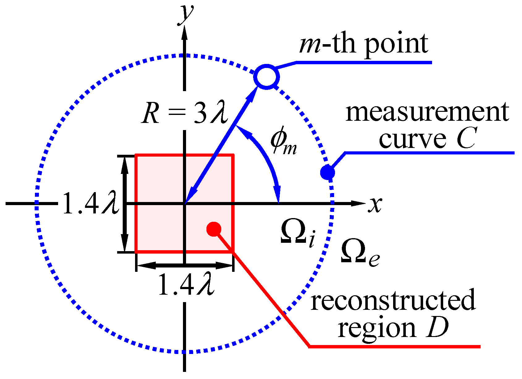
Figure 1 shows an image of the main issues addressed in this paper. A target object is located in the free space with permittivity ε0 and permeability μ0. The entire space is divided into two regions—interior region Ωi and exterior region Ωe—by a closed measurement curve C of radius R. The object is located in Ωi, while the impressed source, unwanted obstacles, and sources of unnecessary waves are placed in Ωe, as shown in Figure 1. We seek to extract the incident field (incoming wave) in region Ωi from the data of total electric and magnetic fields measured along the curve C; the inverse scattering problem can then be analyzed in the usual way.
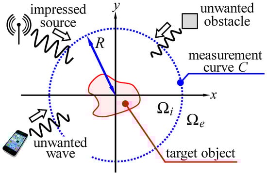
Figure 1.
Image of the main issues addressed here.
2.1. Expansion of Electromagnetic Field by Bessel and Hankel Functions
It is assumed that the object is illuminated by TMz wave (Ez, Hφ), where Ez and Hφ denote the electric field and the magnetic field in the cylindrical coordinate (ρ, φ, z), respectively. As is well known, the incident wave in Ωi can be expressed in terms of Bessel functions Jn as follows [9]:
where αn is the expansion coefficient, is the free-space wavenumber with angular frequency ω, and j denotes the imaginary unit. On the other hand, the scattered wave propagating toward the outside of C can be expanded by Hankel functions of the second kind as follows:
where βn is the expansion coefficient.
Using (1) and (2), and the following equation:
the incident magnetic field and scattered field are, respectively,
where denotes the wave impedance in the free space, and the derivatives of Bessel and Hankel functions are calculated by:
The unknown expansion coefficients αn and βn can be obtained by integrating the fields along the measurement curve C or by solving a matrix equation with respect to the coefficients described in the following subsections.
2.2. Determining the Expansion Coefficents by Integral
Total field measured at point (R, φ) on curve C can be expressed by the sum of incident and scattered field as follows:
Substituting (1), (2), (4) and (5) into (8), the equation with unknown variables αn, βn can be derived as follows:
Multiplying (9) by e−jmφ and integrating over [0, 2π] with respect to φ, we obtain:
Here, the following orthogonality relations:
are used for the formulation of (10). By solving (10) and using the formula of cylindrical functions that , the unknown coefficients are formulated as follows:
2.3. Determining the Expansion Coefficents from Matrix Equation
The expansion coefficients can be also obtained by solving a simple set of linear equations based on (9). If we approximate the sum of the infinite series of Bessel and Hankel functions by a sum of finite 2N + 1 terms (N is a natural number) and measure the total field at M points on the curve C, then (9) is reduced to:
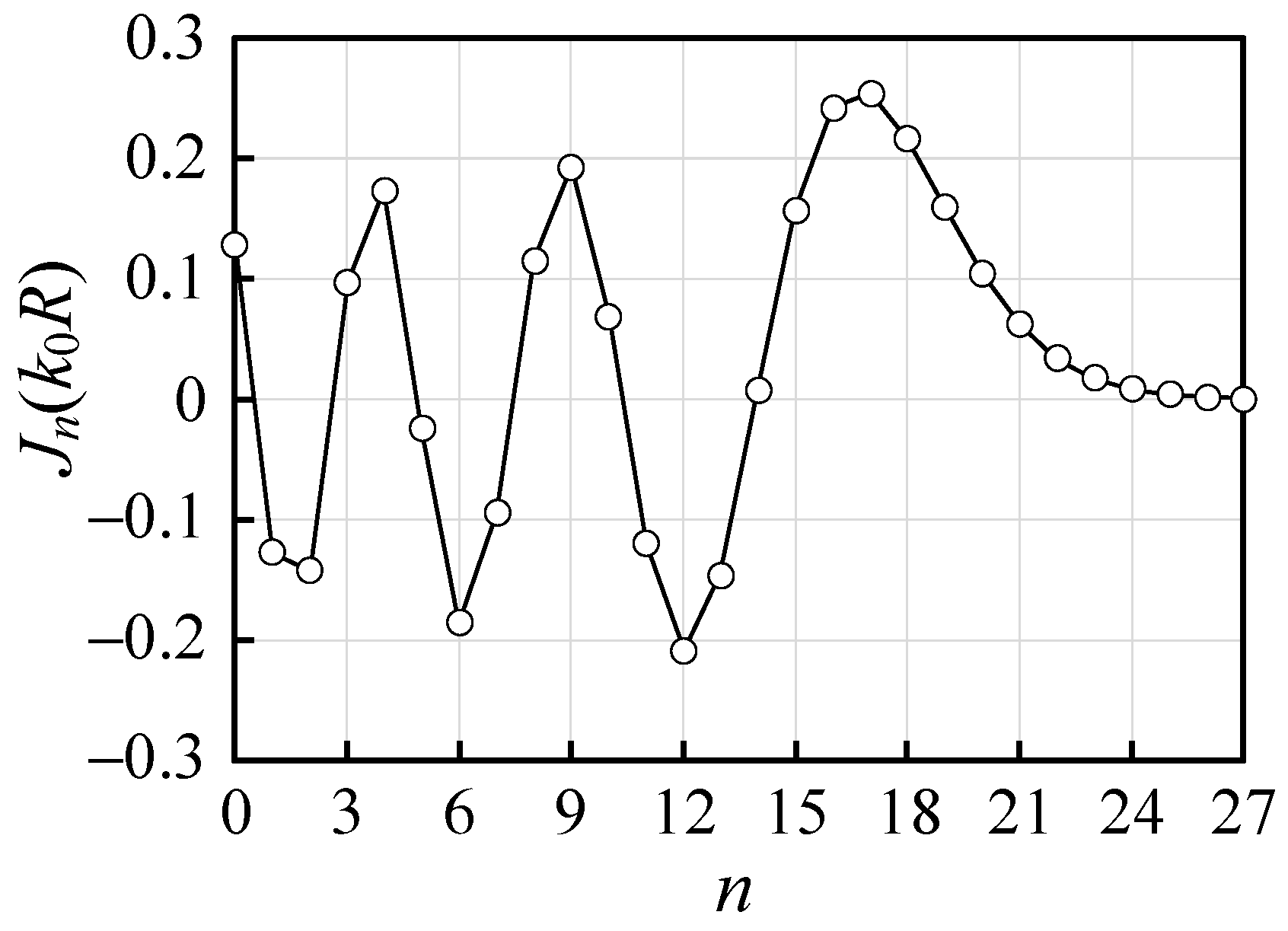
The truncation number N can be determined from variation of Bessel function Jn(k0R) with respect to order n, when the value k0R is constant. For the case of k0R = 6π, as shown in Figure 2, when n is larger than 24, Jn(k0R) approaches to zero. In this case, it can be seen that N > 24 is appropriate.
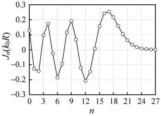
Figure 2.
Variation of Bessel functions (R = 3λ, λ = 3 cm).
On the other hand, the angular coordinate of the m-th measurement point φm is determined by:
When M = 2N + 1, the set of linear Equations (14) has a unique solution. If M > 2N + 1, αn and βn are determined by the least-squares technique.
3. Inverse Scattering Problem
Figure 3 shows the geometrical configuration of the inverse scattering problem. We sought to reconstruct the contrast function:
at point r = (x, y) in the square domain D, including unknown object, where εr and σ denote the relative permittivity and conductivity, respectively. It is assumed that region Ωi is illuminated L times by different sources located outside, and for each time the total fields are measured at M points on the measurement curve C.

Figure 3.
Geometrical configuration of the inverse scattering problem.
The inverse scattering problem is reduced to an optimization problem, in which the following cost functional is minimized:
where K is the normalization factor:
denotes the measured electric field, and denotes a measurement point. Total field is derived by solving this integral equation:
where denotes the Green function of the background medium, given by
with the zero-order Hankel function of the second kind. We use the information on incident field extracted from the measured total electric and magnetic fields for , the first term on the right side of (19).
The conjugate gradient method is used to minimize the functional F(χ). The gradient of F(χ) can be formulated by the Frèchet differential of F(χ), and the gradient g(r) is found to be
where * denotes the complex conjugate. Here, the function satisfies the following adjoint equation:
In this paper, the search for the direction vector is based on the Polak-Ribière-Polyak method [10], and the step size for updating the contrast is determined by the golden section method [10]. The total field and adjoint field are calculated by applying the method of moments (MoM) [11,12] to integral equations.
4. Results and Discussion
In this paper, we use a plane wave to illuminate the object:
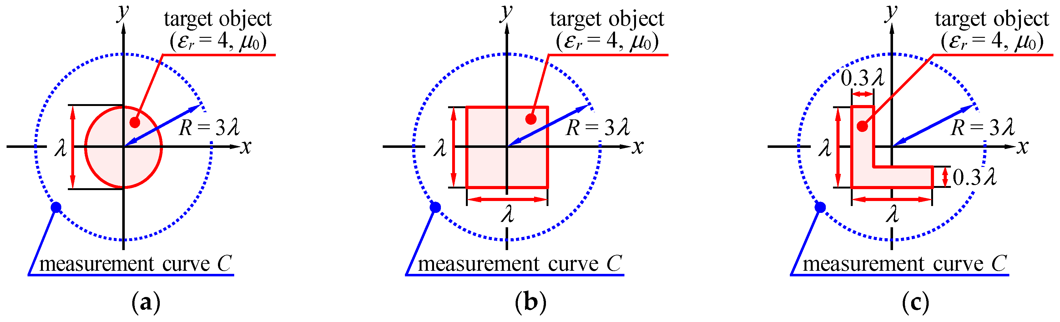
The free-space wavelength is λ = 3 cm. The effectiveness of the proposed method is confirmed by numerical examples with three types of lossless objects shown in Figure 4. The measurement data are collected by numerical simulations based on MoM, where the region Ωi containing the target is divided into small square cells with width of λ/30. The key point is how accurately can the information of the incident field be extracted from the measured data of total fields. Therefore, noise-free data are used in all numerical simulations:
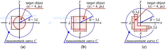
Figure 4.
Shape of target object: (a) cylinder, (b) square, and (c) L-shape.
4.1. Accuracy of Extracted Incident Field
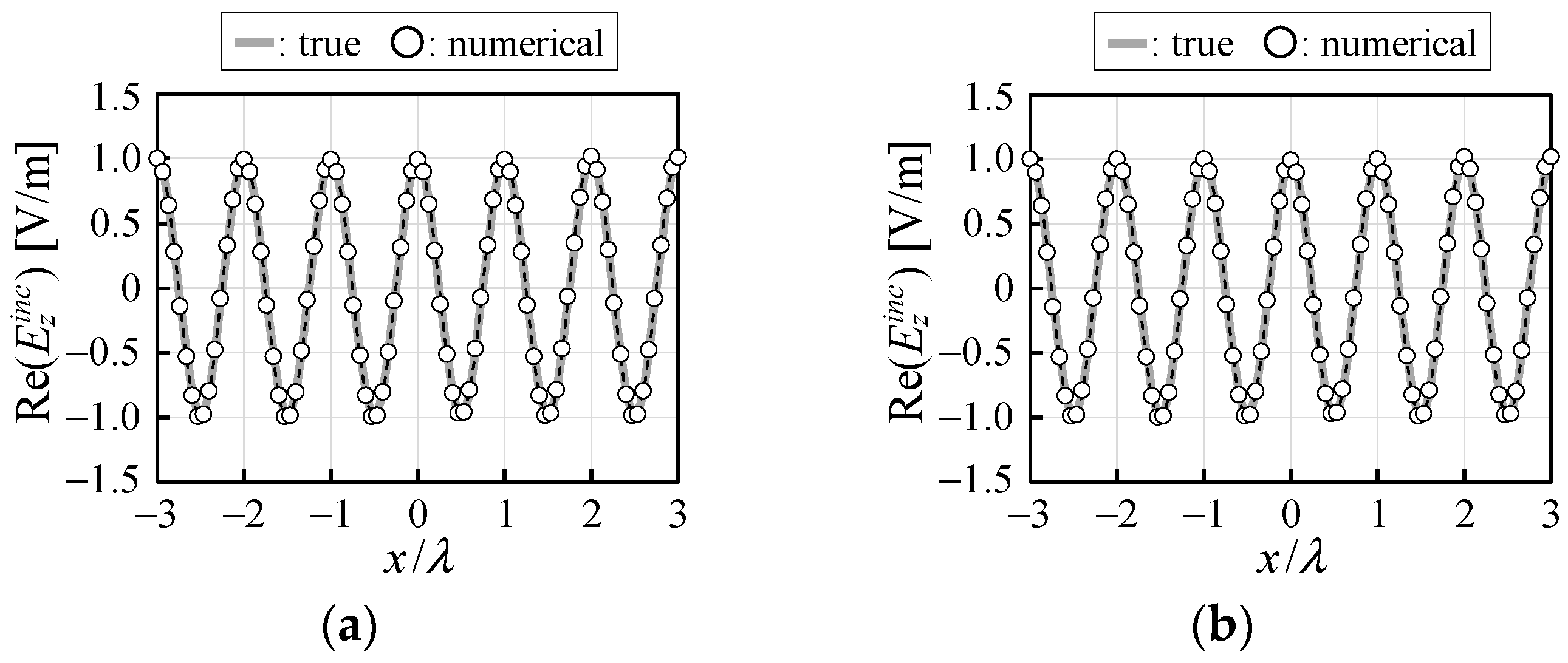
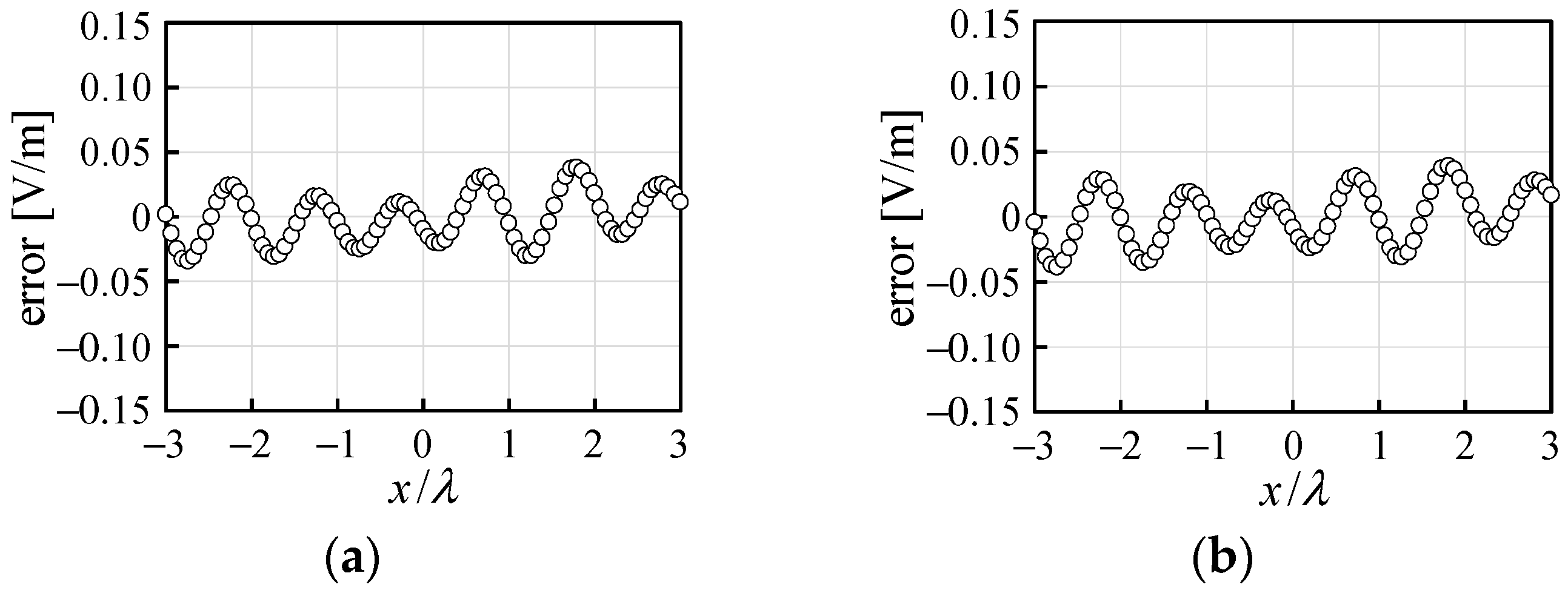
Figure 5 shows the real part of the incident wave extracted from measured data of total fields for the case of a cylindrical object, as shown in Figure 4a. The values of the incident field inside the measurement curve were calculated by (1) with αn determined from the solution of linear Equation (14). The results shown in Figure 5a–c have an error of ±0.12 V/m, ±0.08 V/m, and ±0.04 V/m, respectively. Here, the error means the difference between the real part of the extracted incident field and that of the reference (true) one , i.e., . The error of the imaginary part of the incident electric field is almost the same variation as the real part. Figure 6 and Figure 7 show the distribution of incident field on x-axis and its error, respectively. The error is decreased by increasing M, as shown in Figure 7.
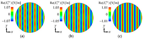
Figure 5.
Extraction results of incident wave in Ωi (target is cylinder): (a) M = 51, (b) M = 100, and (c) M = 200.
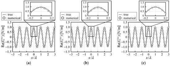
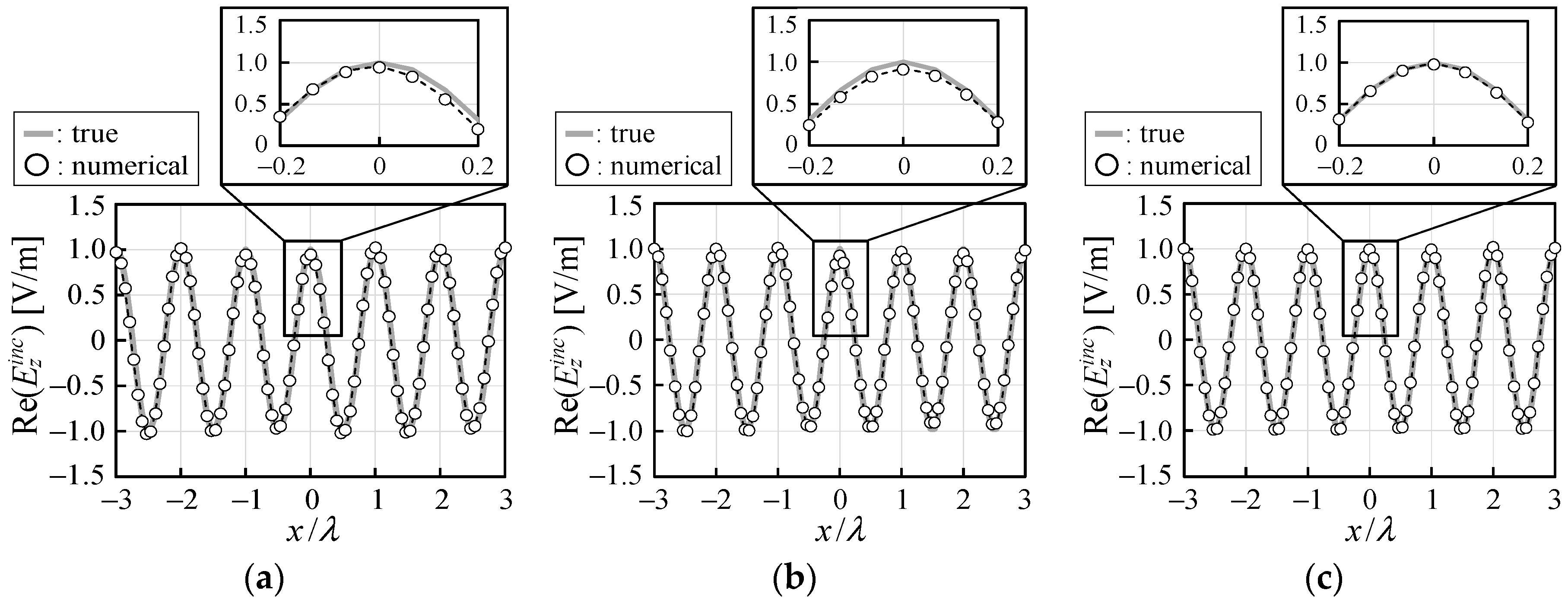
Figure 6.
Distributions of incident field on x-axis (target is cylinder): (a) M = 51, (b) M = 100, and (c) M = 200.
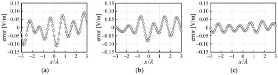
Figure 7.
Error of incident field on x-axis (target is cylinder): (a) M = 51, (b) M = 100, and (c) M = 200.
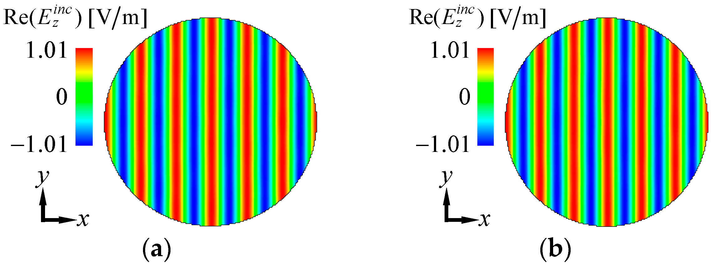
In the case of the square or L-shape object, the incident field is also successfully estimated by setting M = 200, as shown in Figure 8, Figure 9 and Figure 10.

Figure 8.
Extraction results of incident field in Ωi (M = 200): (a) square target and (b) L-shape target.

Figure 9.
Distributions of incident field on x-axis (M = 200): (a) square target and (b) L-shape target.

Figure 10.
Error of incident field on x-axis (M = 200): (a) square target and (b) L-shape target.
4.2. Reconstruction of Target Object Using Extracted Incident Field
In this section, the performance of the proposed method is verified on inverse scattering problems, where relative permittivity εr is estimated. From the results in the preceding Section 4.1, M is set to 200, and the cost functional F is evaluated on the measurement curve C of radius 3λ. The initial εr in the reconstructed region is set to 2.0, i.e., initial contrast χ(0) = 1.0. It is assumed that we illuminate the target with the plane wave:
from L = 15 directions, where θl denotes the incident angle:
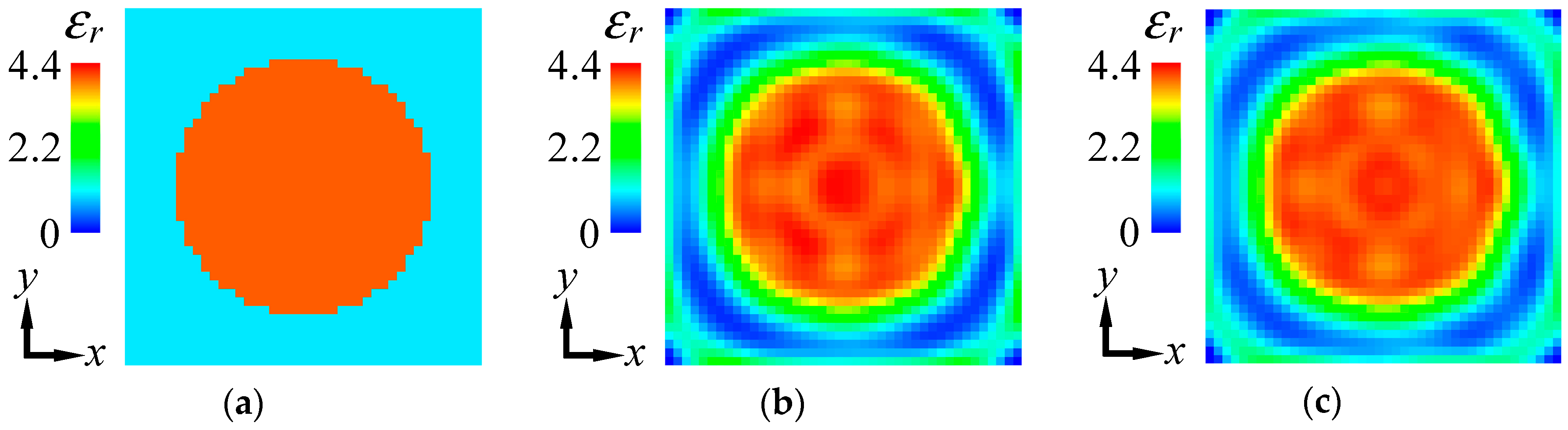
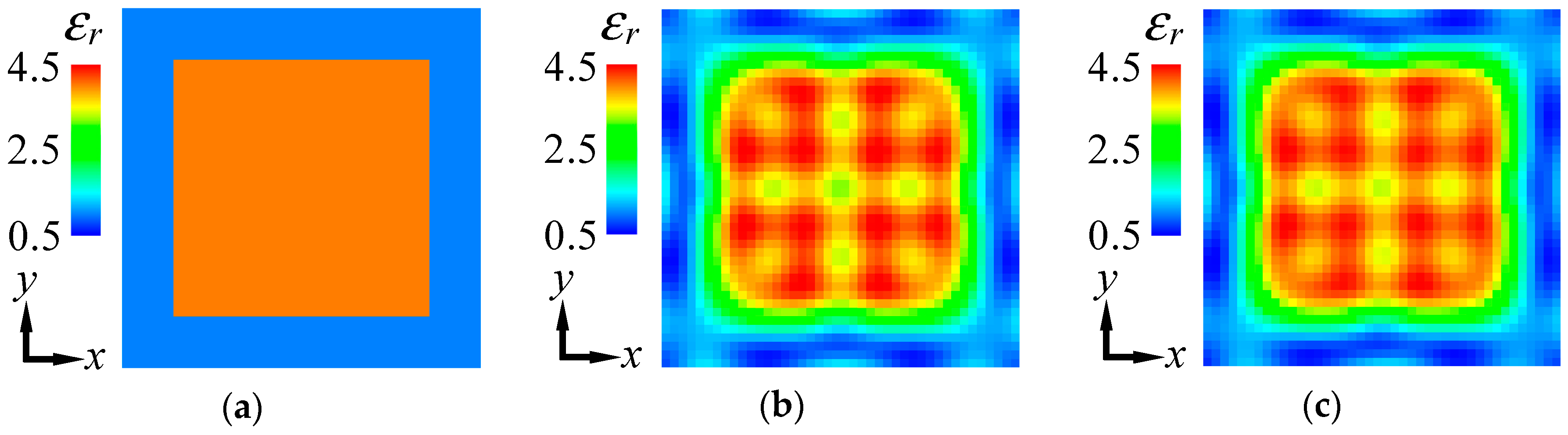
The first example is a reconstruction of the cylindrical object. The reconstructed images after 50 iterations are shown in Figure 11. The relative-permittivity distributions matching the original profile are obtained. Comparing (b) and (c), it can be seen that the proposed method is effectual in inverse scattering analysis from measurement data of total fields. Next, Figure 12 and Figure 13 show results for the square and L-shape objects, respectively. Similarly, the target objects are successfully reconstructed with and without information on incident field. The accuracy of the reconstructed relative permittivity is evaluated by means of the root mean square reconstruction error (RMSE) defined by:
where are and are the reconstructed relative permittivity and the reference one, respectively. S is the number of cells in reconstructed region D, as shown in Figure 3. Table 1 lists the RMSE. The accuracy of reconstruction using the extracted incident field is almost comparable with that using the true incident field.
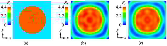
Figure 11.
Reconstruction results for the cylindrical object after 50 iterations: (a) true image, (b) reconstructed image using information on the exact incident field, and (c) reconstructed image using information on the extracted incident field.

Figure 12.
Reconstruction results for the square object after 50 iterations: (a) true image, (b) reconstructed image using information on the exact incident field, and (c) reconstructed image using information on the extracted incident field.
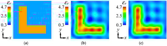
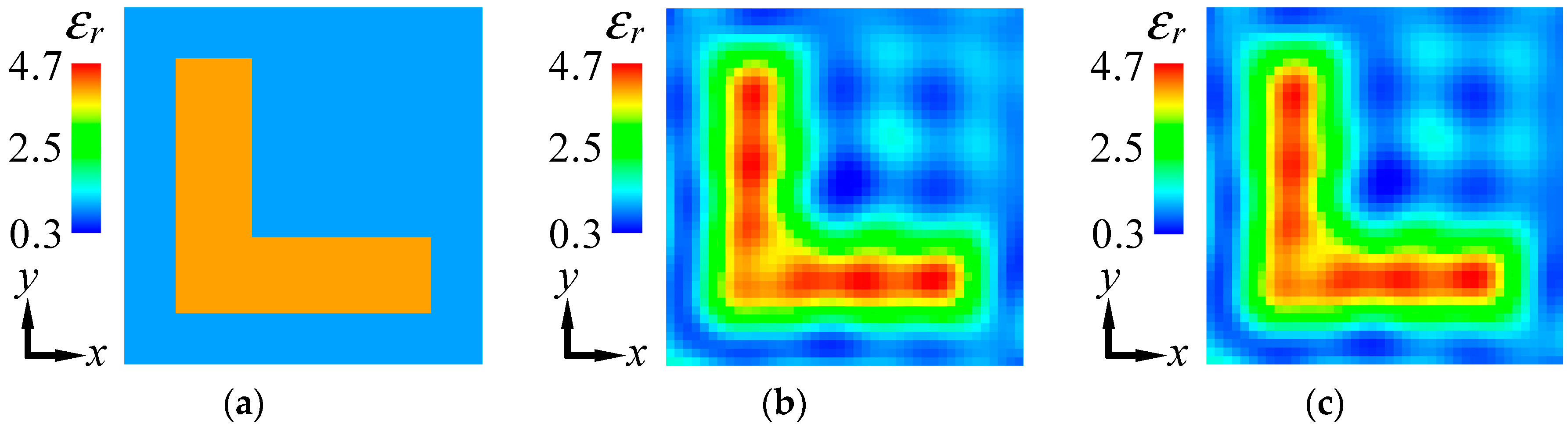
Figure 13.
Reconstruction results for the L-shape object after 50 iterations: (a) true image, (b) reconstructed image using information on the exact incident field, and (c) reconstructed image using information on the extracted incident field.

Table 1.
Reconstruction errors.
4.3. Inverse Scattering Analysis with Unwanted Obstacles
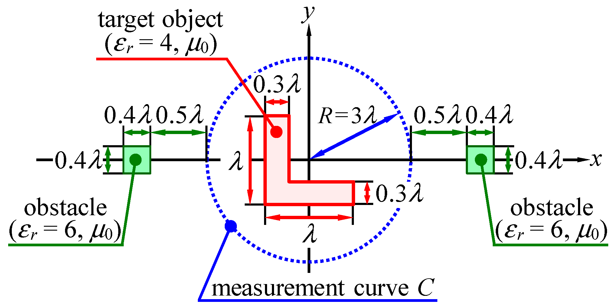
Finally, the effectiveness of the proposed method is confirmed by a problem where there are unwanted obstacles. Figure 14 shows the geometry of the problem. There are two square obstacles outside the measurement curve C. Usually, it is necessary to include all obstacles in the computational domain of inverse scattering analysis, such that the computational domain is expanded to a much larger size, and lots of computing resources are exhausted. Using the proposed method, the incident wave, including the wave scattered by obstacles, are extracted from the data of total fields measured along the curve C. Therefore, there is no need to expand the computational domain and the resources can also be saved. Here, the measured total fields are obtained by simulation, in which the target object and obstacles are irradiated by the plane wave.
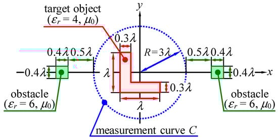
Figure 14.
Geometry of inverse scattering analysis including unwanted obstacles.
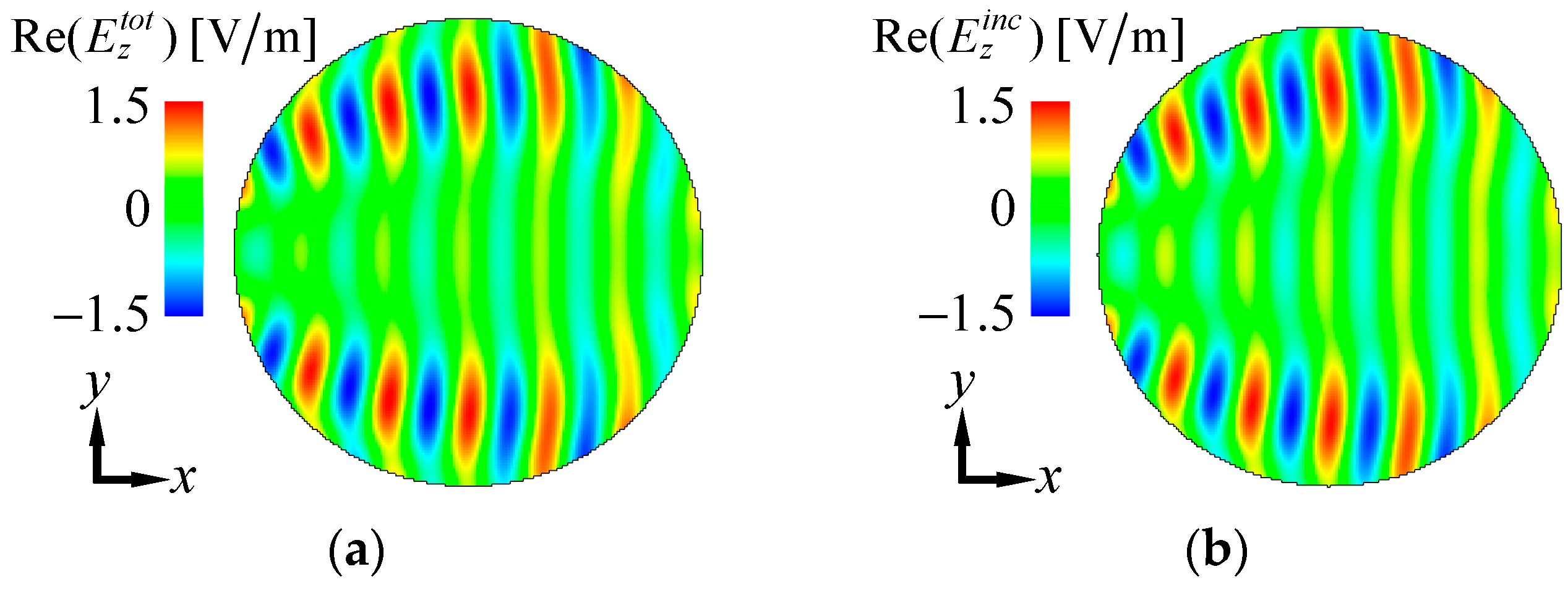
Figure 15 shows the extraction results of the incident field where incident angle θl is zero. To confirm the accuracy of the extracted field, the total field derived from simulation, where the target object is removed and obstacles are included in the computational domain, is shown in Figure 15a. It can be seen that the incident field can be estimated even if there are unwanted obstacles outside the measurement curve. Figure 16 shows the reconstruction results. The relative-permittivity distribution of the target object is successfully reconstructed by the inversion algorithm with the proposed method.
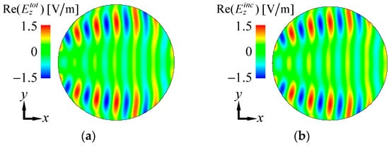
Figure 15.
Extraction result of incident field with unknown obstacles: (a) total field obtained by simulation, where the target object is removed and obstacles are included in the computational domain, and (b) extracted incident field with the proposed method (M = 200).
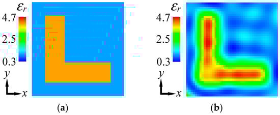
Figure 16.
Reconstruction results of a situation where two unwanted obstacles exist in the exterior region Ωe: (a) true image and (b) reconstructed image using information on the extracted incident field.
5. Conclusions
In this paper, a method for extracting incident field from the measured data of total electric and magnetic fields has been proposed. The incident field can be easily estimated by means of cylindrical-wave expansion. The extracted field has sufficient accuracy if enough information about the total fields on the measurement curve is available.
The proposed method has been applied to inverse scattering problems. Unknown objects are successfully reconstructed by the developed method. Furthermore, it is shown that the proposed method is effectual even if unwanted obstacles exist outside the measurement curve.
In this paper, many measurement points are required for field extraction. For practical application, it is useful to reduce the measurement point. One of the approaches employed uses FFT and zero padding techniques as data interpolation; this will be done in future research. In addition, we examined only cases where the measurement curve was a circle. However, it could be of any other shape as well or an open curve in actual problem. This examination can also be the focus of future work. Furthermore, lossy case and influence of the measurement error will be investigated.
Author Contributions
T.T. (Tomonori Tsuburaya) performed the research and the simulation; Z.M. developed the research plan, and contributed to provision of the research material and validation of the simulation result; T.T. (Takashi Takenaka) worked on the methodology; T.T. (Tomonori Tsuburaya) wrote the original draft; Z.M. and T.T. (Takashi Takenaka) reviewed the draft.
Funding
This research received no external funding.
Conflicts of Interest
The authors declare no conflict of interest. The funders had no role in the design of the study; in the collection, analyses, or interpretation of data; in the writing of the manuscript, or in the decision to publish the results.
References
- Chew, W.C.; Wang, Y.M. Reconstruction of Tow-Dimensional Permittivity Distribution Using the Distorted Born Iterative Method. IEEE Trans. Med. Imaging 1990, 9, 218–225. [Google Scholar] [CrossRef] [PubMed]
- Joachimowicz, N.; Pichot, C.; Hugonin, J.-P. Inverse Scattering: An Iterative Numerical Method for Electromagnetic Imaging. IEEE Trans. Antennas Propagat. 1991, 39, 1742–1752. [Google Scholar] [CrossRef]
- Kleinman, R.E.; Van den Berg, P.M. A modified gradient method for two-dimensional problems in tomography. J. Comp. Appl. Math. 1992, 42, 17–35. [Google Scholar] [CrossRef]
- Harada, H.; Wall, D.J.N.; Takenaka, T.; Tanaka, M. Conjugate Gradient Method Applied to Inverse Scattering Problem. IEEE Trans. Antennas Propagat. 1995, 43, 784–792. [Google Scholar] [CrossRef]
- Van den Berg, P.M.; Kleinman, R.E. A contrast source inversion method. Inverse Probl. 1997, 13, 1607–1620. [Google Scholar] [CrossRef]
- Franchois, A.; Pichot, C. Microwave Imaging-Complex Permittivity Reconstruction with a Levenberg-Marquardt Method. IEEE Trans. Antennas Propagat. 1997, 45, 203–215. [Google Scholar] [CrossRef]
- Yang, R.; Meng, Z.Q.; Takenaka, T. Extraction of incident field from total field data. In Proceedings of the Progress in Electromagnetics Research Symposium (PIERS), Shanghai, China, 8–11 August 2016; pp. 4073–4077. [Google Scholar]
- Yang, R.; Meng, Z.Q.; Takenaka, T. Conjugate Gradient Method Applied to Inverse Scattering with No Prior Information on Incident Field. In Proceedings of the 2017 Progress in Electromagnetics Research Symposium—Fall (PIERS—FALL), Singapore, 19–22 November 2017; pp. 731–736. [Google Scholar]
- Harrington, R.F. Time-Harmonic Electromagnetic Fields; McGraw-Hill: New York, NY, USA, 1961. [Google Scholar]
- Press, W.H.; Flannery, B.P.; Teukolsky, S.A.; Vetterling, W.T. Numerical Recipes in C: The Art of Scientific Computing, 2nd ed.; Cambridge University Press: New York, NY, USA, 1992. [Google Scholar]
- Richmond, J.H. Scattering by a Dielectric Cylinder of Arbitrary Cross Section Shape. IEEE Trans. Antennas Propagat. 1965, 13, 334–341. [Google Scholar] [CrossRef]
- Harrington, R.F. Field Computation by Moment Methods; Wiley-IEEE Press: New York, NY, USA, 1993. [Google Scholar]


© 2019 by the authors. Licensee MDPI, Basel, Switzerland. This article is an open access article distributed under the terms and conditions of the Creative Commons Attribution (CC BY) license (http://creativecommons.org/licenses/by/4.0/).