Article

Implementation of Pattern Recognition Algorithms in Processing Incomplete Wind Speed Data for Energy Assessment of Offshore Wind Turbines

1
Department of Electrical Engineering, Technological Educational Institute of Thessaly, 41110 Larisa, Greece
2
Department of Civil Engineering and Geomatics, Cyprus University of Technology, 3036 Limassol, Cyprus
3
Department of Civil Engineering, Aristotle University of Thessaloniki, 54124 Thessaloniki, Greece
*
Author to whom correspondence should be addressed.
Electronics 2019, 8(4), 418; https://doi.org/10.3390/electronics8040418
Submission received: 26 March 2019 / Revised: 6 April 2019 / Accepted: 8 April 2019 / Published: 10 April 2019
(This article belongs to the Section Artificial Intelligence)

Abstract

:
Offshore wind turbine (OWT) installations are continually expanding as they are considered an efficient mechanism for covering a part of the energy consumption requirements. The assessment of the energy potential of OWTs for specific offshore sites is the key factor that defines their successful implementation, commercialization and sustainability. The data used for this assessment mainly refer to wind speed measurements. However, the data may not present homogeneity due to incomplete or missing entries; this in turn, is attributed to failures of the measuring devices or other factors. This fact may lead to considerable limitations in the OWTs energy potential assessment. This paper presents two novel methodologies to handle the problem of incomplete and missing data. Computational intelligence algorithms are utilized for the filling of the incomplete and missing data in order to build complete wind speed series. Finally, the complete wind speed series are used for assessing the energy potential of an OWT in a specific offshore site. In many real-world metering systems, due to meter failures, incomplete and missing data are frequently observed, leading to the need for robust data handling. The novelty of the paper can be summarized in the following points: (i) a comparison of clustering algorithms for extracting typical wind speed curves is presented for the OWT related literature and (ii) two efficient novel methods for missing and incomplete data are proposed.

1. Introduction

1.1. Motivation and State-of-the-Art

During recent decades, the utilization of wind power has witnessed a growth that is close to 25%, a fact that indicates that wind power is a significant contributor to electricity generation across the globe [1]. This progress is due to both the high wind resource availability and the technology maturity of wind energy compared to other renewable energy resources [2,3]. Offshore wind installations have become an attractive option due to the enormous energy potential associated with the vast offshore areas. They provide a set of advantages compared to their onshore counterparts including higher productivity per installed unit, less visual impact and noise, an absence of limitations of the onshore geography, and low carbon emissions during their life-cycle to name several [4,5]. Offshore wind turbines can serve as sole generation units [6,7], or can be hybridized with wave energy converters [8,9,10].
The selection of the installation site is subject to many diverse criteria such as water depth, environmental impact, seabed characteristics, wind resource, and the minimum distance to the high voltage grid among others [11]. Thus, special care should be taken with respect to decision-making analysis in order to clarify the attributes of each site and the potential capacity of each wind system. While offshore wind farms continually gather the interest of investors, construction companies, utilities, grid operators, self-producers and others, accurate on-site measurements and studies are crucial to the success of offshore wind farms. Due to technical drawbacks or other random events, accurate and complete measurements of renewable energy source sites are not always feasible. This fact raises difficulties with respect to techno-economic evaluation and feasibility studies. Therefore, it is a challenging engineering problem to develop tools to cope with the incomplete measurements, and to provide a reliable base to support the techno-economic evaluation of possible future OWTs.
It is very common that real measured data are not perfect and contain incomplete or missing data. For the purposes of the present paper unmeasured data sets at various periods within a day correspond to the term incomplete data, while no measured data sets for one day correspond to the term missing data, i.e., time or other series with missing entries. The presence of missing measured data in any possible data set could affect the assessment of the performance of any structure/system if these data sets were used as input. For the case that the rate of missing data in a sample of data is less than 1% then generally these missing values are considered trivial, while if the rate is between 1–5% then the missing data are manageable. For the case in which rate is between 5–15%, sophisticated methods are required for handling this phenomenon [12].
Missing data cases are treated in three ways: (a) discard the series with missing data from the available set, (b) utilize maximum likelihood processes based on the measured data and (c) substitute missing data with estimated or artificial ones. In most cases, measured data set attributes are not independent from each other and relationships among attributes exist for data in different time period. The methods that have been applied for completion of missing data are the K-Nearest Neighbor [13], Concept Most Common Attribute Value for Symbolic Attributes [14], K-means Clustering [15], Fuzzy K-means Clustering [16], Event Covering [17], Regularized Expectation-Maximization [18], Support Vector Machines [19], Singular Value Decomposition [20] and Bayesian Principal Component Analysis [21]. According to [22], the Event Covering method offers a very good synergy with Radial Basis Function Networks for missing data. According to [23], there is no universal substitute method for missing data that performs best for all classifiers. In [24] time series of wave height data with 16.50% and 33% missing values are filled with the use of a method that is based on the nonstationary modeling of long-term time series by means of simulated data from a population of data with the same probability law. The Data Interpolating Empirical Orthogonal is proposed in [25] to reconstruct missing data from satellite images, which is especially useful for filling missing data from geophysical fields.
In [13], the K-Nearest Neighbor (KNN) method is applied into four sets, Bupa, Cmc, Pima and Breast obtained by the UCI Repository of Machine Learning Datasets. The authors discuss the poor performance in KNN in the Breast set; thus, while KNN is effective in the other three sets, it cannot be used in all sets. Also, according to the authors, another limitation is the high computational cost of the KNN. In [14], the method is applied in medical data. The missing data entry is filled with the average of all values of the corresponding attribute, i.e., the corresponding element, if data are expressed as vectors. This approach is sensitive to outliers. Further, according to the authors, the consistency level (i.e., the amount of missing data) of the data set highly affects the performance of the filling method. In [15], the method is tested on weather and medical data and is built upon the K-means algorithm. No discussion is provided about the attributes of the sets and the data dimension. The method’s performance is affected by the amount of the missing data and does not always outperform the benchmark algorithm that is used for comparison. In [16], the proposed method does not always present the best results among others that are examined. In [17,18], the proposed methods lead to promising results for data with two entries but there is no discussion of multi-dimensional data. In [19], the method is tested on medical data. The authors do not provide metrics on the model’s performance. In [20], the authors present a method based on Singular Value Decomposition (SVD). The authors state that its performance is sensitive to the type of data being analyzed and the method yields best results on time-series data with low noise level. In [21], the authors investigate the application of a Bayesian Principal Component Analysis (BPCA) method in gene expression profile data. The BPCA is compared with KNN and SVD and leads to better results. The authors discuss the drawbacks of the BPCA, i.e., the estimation with BPCA may not be accurate if genes have dominant local similarity structures. In such a case, the KNN is suitable. The hybrid model of [22] is tested in a variety of data sets and leads to satisfactory results. The main limitation is the increased computational cost. In [24], the authors deal with wave data and the data filling takes place in three-hour intervals. In [25], the method is used for recovering images from a satellite; however, no evaluation metrics are used for the method’s performance.
Because in most cases wind speed measured series exhibit nonlinearities and complexity, pattern recognition algorithms are robust candidates to be included in the proposed methodology. More specifically, various clustering algorithms are utilized to cluster the available wind speed data set into compact and well-separated clusters. Clustering is suitable in cases where no formal and prior knowledge of the data inter-relationships is available [26,27]. The clustering procedure is purely data-driven; the optimal number of clusters is defined by mathematical criteria measuring the similarity between the data objects. The output of clustering leads to groups with a high similarity between their members. Each group constitutes a profile which is the representative member of the cluster. Actually, clustering provides a reduction of the initial data set to a set of reduced patterns (i.e., the profiles) that describes the data set. Clustering has been successfully implemented in a variety of pattern recognition problems [28]. In [29], clustering is applied to patterns that contain two elements. The first refers to the ratio of the average daily wind speed to the average monthly wind speed. The second element corresponds to the Hurst indicator calculated for the average daily values. The algorithm used is the Fuzzy C-means. The data cover a period of three years. In [30] the data have been collected from an on-shore park in USA and cover a period of a year. The scope is to the present a methodology for estimating the power curve of a wind turbine. The clustering algorithm used is the K-means. Authors of [31] focus on the wake effect analysis by providing a comparison between three clustering algorithms. In [32] the K-means algorithm is used to cluster patterns that are composed by pairs of wind speed and generated power. The K-means algorithm is also used in [33]. The data are drawn from two meteorological stations in Mexico. The patterns used in clustering contain the wind speed and direction. The hierarchical Ward algorithm is employed in [34]; the patterns elements are wind speed, velocity and vorticity. In [35,36] clustering is used as supportive stage of wind power forecasting.
The rest of the paper is structured as follows: Section 2 contains the description of methods proposed in the paper. Specifically, the clustering process is described together with the methods of missing and incomplete data filling, respectively. The results are analyzed in Section 3. Section 4 provides a discussion on the results and finally, Section 4 provides the main conclusions of the paper and some direction for future research.

1.2. Contribution of the Present Paper
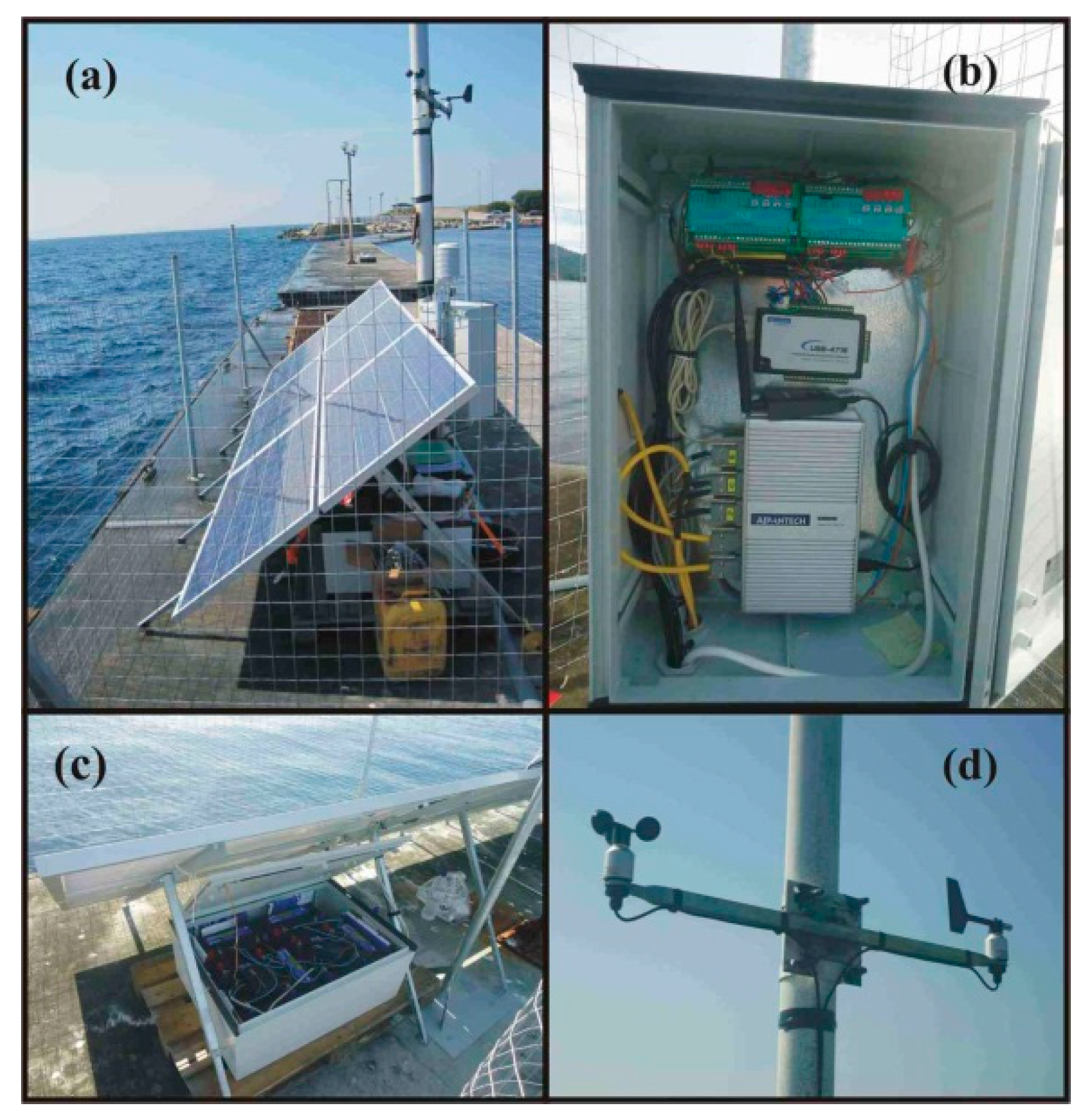
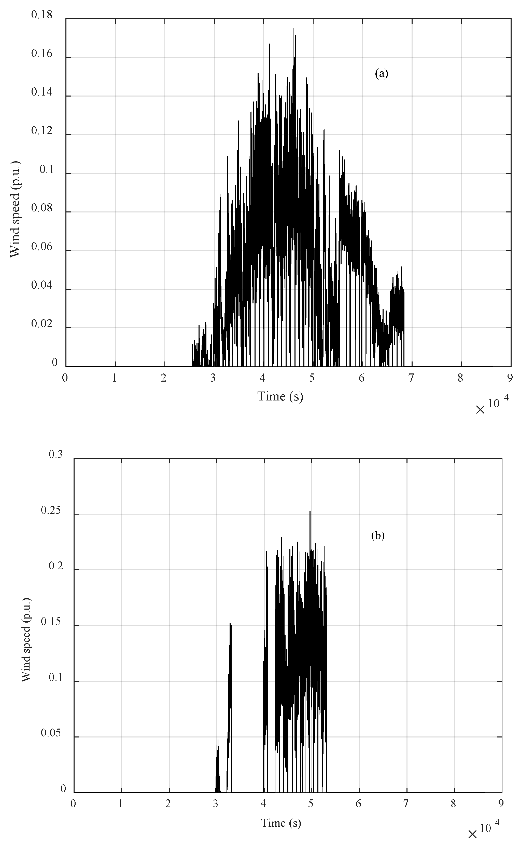
Based on the above brief literature survey, it is obvious that the filling problem of incomplete and missing data needs further investigation and experimentation. The basic shortcomings of the literature can be summarized as: (i) Some methods are not examined in high dimensional data, and (ii) some methods correspond to high computational cost. The literature on missing data treatment is mainly focused on medical data. No attention is placed in renewable energy resources such as high-resolution wind speed time series. Also, no potential applications are discussed.
The aim of this paper is to develop methodologies for filling incomplete or missing wind speed data sets. The developed methodologies are applied on a set of real offshore site measurement that serves as the test case in Neos Marmaras, Greece. Part of the data of the test case serves for the validation of the proposed methodologies. The complete time series of the wind speed set are afterwards used for the assessment of the produced power of a specific offshore wind turbine type in the same location.
The objectives of this work can be summarized as follows:
(a)
This study is structured around the problem of working with incomplete and/or missing data; since this situation is frequent in renewable energy assessment preliminary studies. Incomplete and missing data pose restrictions on the techno-economic assessment of renewable energy projects. With the present paper, methodologies on investigating methods to overcome the aforementioned restrictions are developed and proposed. Two novel proposed methods for filling missing and incomplete wind speed data are developed, implemented and tested against real measured data that are obtained from a monitoring system installed in Neos Marmaras, Greece.
(b)
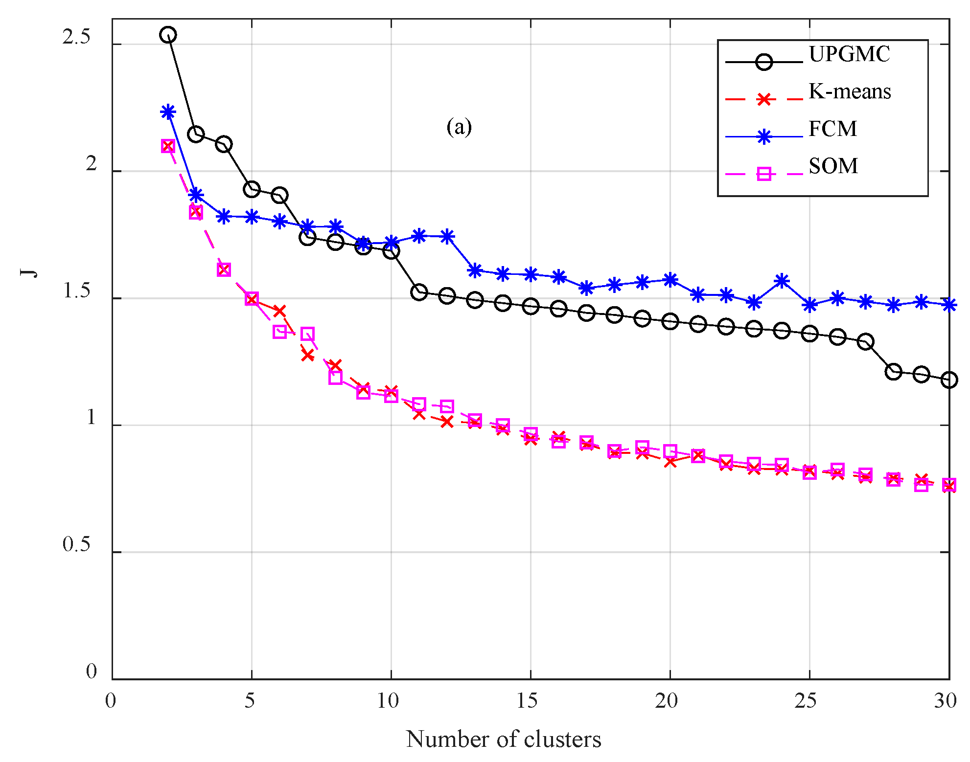
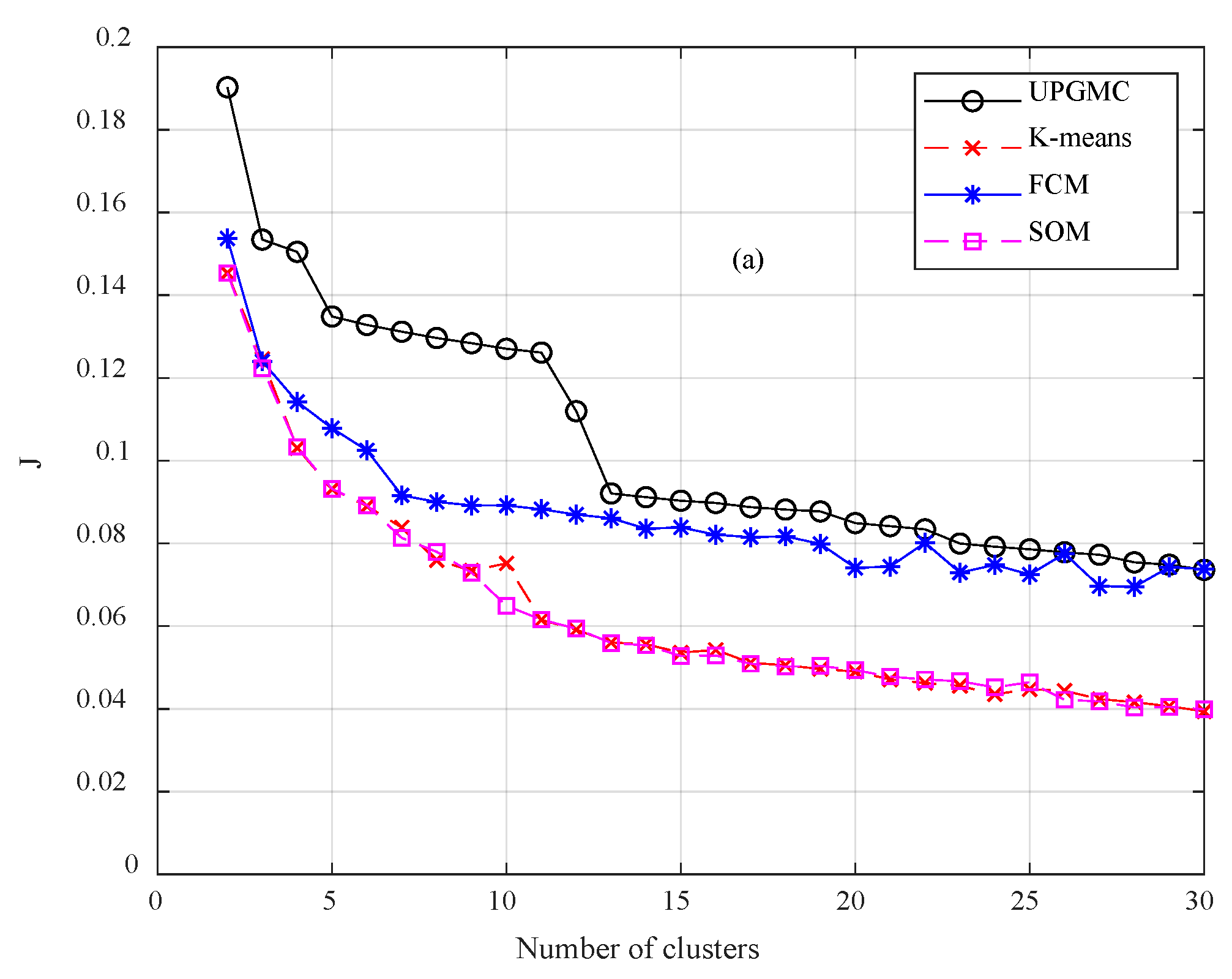
The utilization of clustering algorithms in wind speed data partitioning has not sufficiently examined in the technical literature. Clustering leads to several advantages in time series modeling. In this study, a comparative analysis takes place between four well researched algorithms. By examining the outputs of clustering, useful conclusions can be drawn for the variations and special attributes of the speed data.
(c)
After the completion of the missing and incomplete data, the energy potential of the specific offshore site is estimated.
To sum up, the paper investigates the usage of computational intelligence algorithms for incomplete and missing wind speed data processing. This processing leads to useful conclusions about the energy potential of a specific region. The aim is to exploit this kind of data for sizing prospective offshore wind generation systems.

2. Materials and Methods

Clustering can aid the development of a descriptive model of the data, i.e., the initial data set can be represented and described by a reduced set of typical wind speed curves or wind speed profiles. Therefore, it is important to examine various clustering algorithms to provide accurate clustering results. The validation of the algorithms is held with a set of validity indicators that measure the compactness of clusters. Both the incomplete and missing data methods are built on clustering. The rationale of this concept is the speed and reduced complexity. In general, the execution of a common clustering algorithm is fast in modern PC system configurations. Also, the proposed incomplete and missing data filling methods do not rely on the utilization of further data apart from the wind speed curves themselves and also, apart from clustering, they do not require further mathematical techniques such as distribution fitting, statistics, data transformation and others. It should be noted that they authors have not tested other incomplete and data missing methods since the scope of the paper is to present the background of two methods and their applications on a real-world data set. A comparison with other methods, if it is feasible, is a direction for future study.

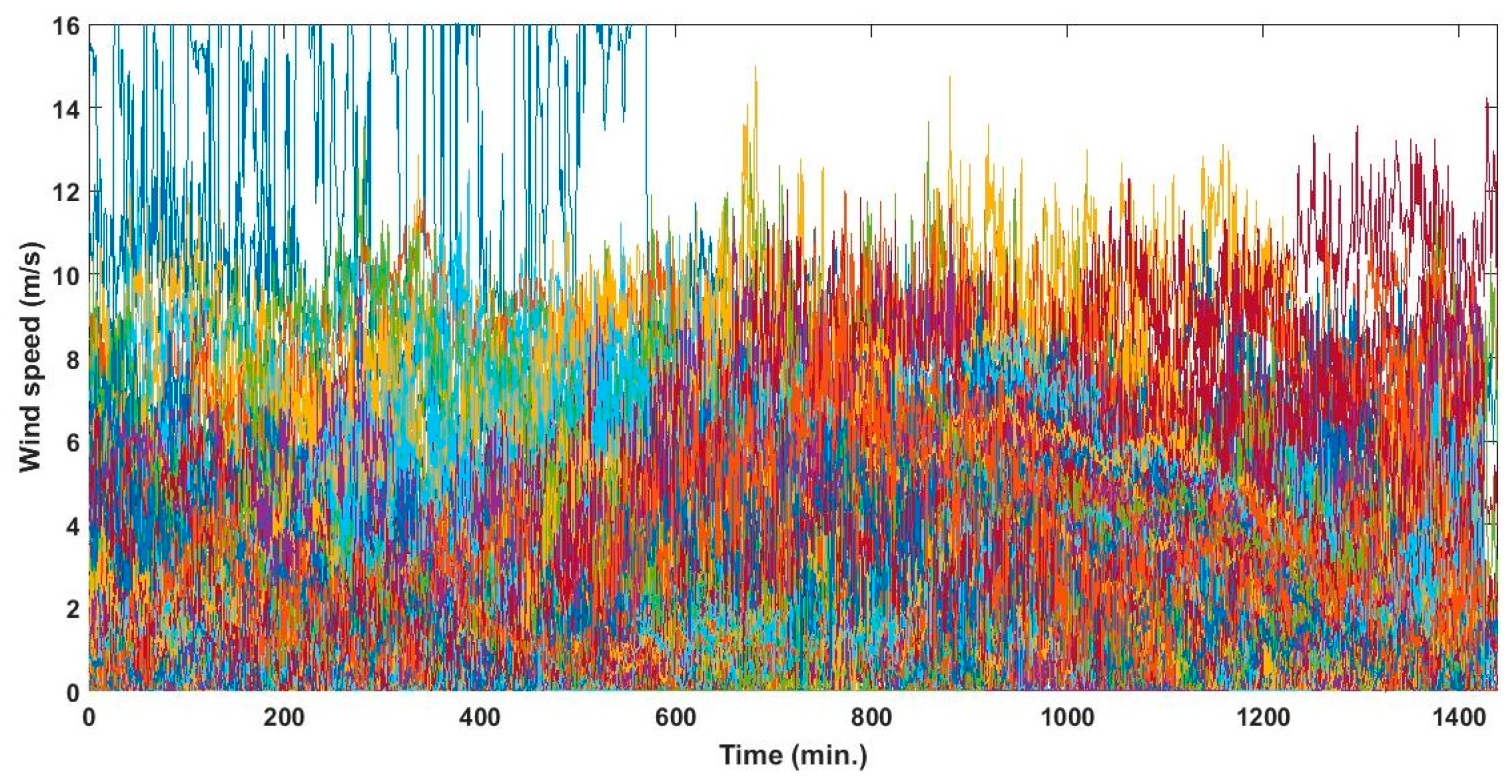
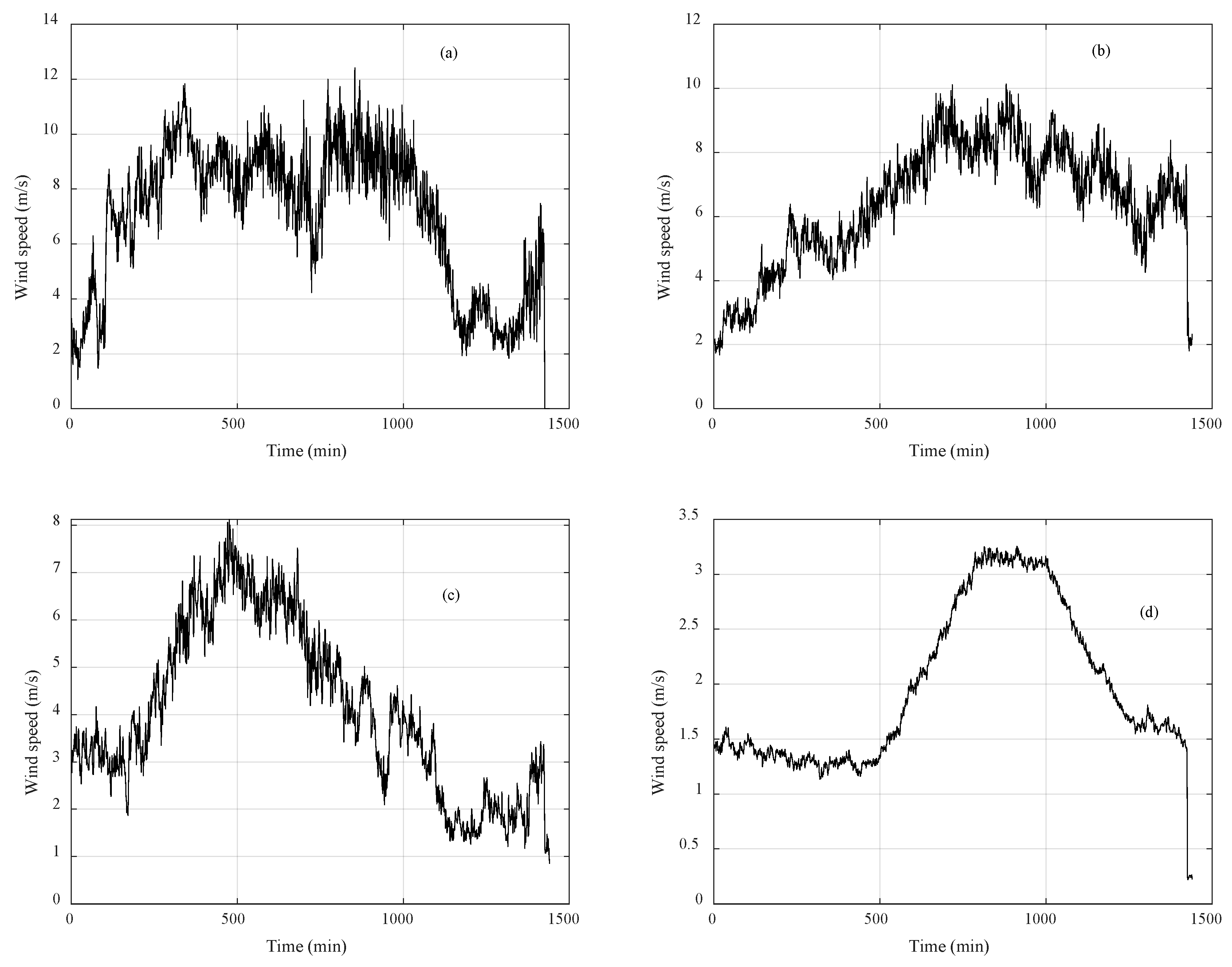
2.1. Description of the Available Data

The wind speed data used in the present paper refer to the period from 28/09/2012 to 23/12/2013, i.e., the period covers 452 days. Among them, 234 and 112 days have complete and incomplete measurements, respectively. The incomplete data refer to partial values, i.e., there are missing data at various periods within the day. In the majority of the days, these periods differ from one day to another. Also, the number/size of missing data usually differs. For the remaining 106 days, no measured data are available, reducing the actual data set to 346 days; these days are described with the term missing. Most of the days with no measured data are placed in the period between 01/09/2013 and 24/12/2013.
The measured wind data are obtained by a Sensor Network for Monitoring the Response (SNMR) deployed on a floating structure operating as a floating breakwater at a water depth of 20 m and located 300 m off the coast of Neos Marmaras, Greece [37,38]. The weather station is capable for recording the wind speed, air temperature, wind direction, humidity and atmospheric pressure. Part of the SNMR in connection with the wind speed measurement is showed in Figure 1. The sampling rate of the measured quantities is considered as 1 Hz.

2.2. Introduction with Regard to Clustering Process

Clustering is an unsupervised machine learning tool that is suitable for cases where there is no or limited information about the structure of a given data set. The data can be grouped together in homogenous clusters where the data within the same clusters present higher similarity compared to the rest. Through the implementation of clustering algorithms, more insightful and exploitable information about the relationships between the data can be formed, and hence a descriptive model of the data can be built. For the purpose of applying the clustering tool affectively, three conditions should be satisfied [26]: (i) suitable representation of the data, (ii) robust clustering algorithm and (iii) robust clustering validation framework.

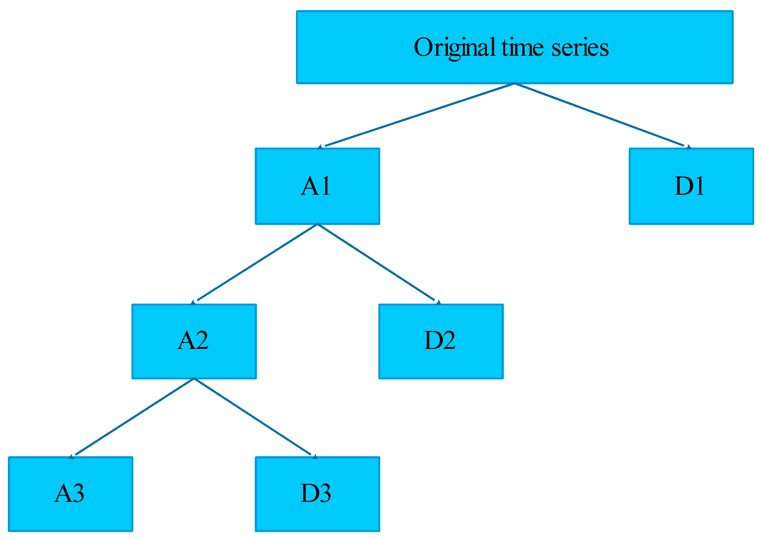
2.3. Patterns Representation

The proper representation of the data is necessary for the application of the algorithms. In the present paper, the clustering is applied on the daily wind speed curves. We refer to the term “pattern” as a finite vector of wind speed values. Each pattern is indicated as p m = [ p m 1 , ... , p m D ] T , where d = 1 , 2 , ... , D is the dimension of the sample. The set of the pattern is denoted as P = { p m , m = 1 , ... , M } , with M indicating the number of the patterns. Also, we denote the maximum value of P as p m max . Since clustering deals with the similarity of of wind speed curve shapes and not with the wind speed levels, we need to normalize the vectors in the [0,1] range by using the following expression [26]:
x m = p m p m max
with the above equation, all patterns are normalized in the [0,1] scale by the division with the base value, which is the maximum value of the set P , i.e., p m max . The set of the normalized patterns is denoted as X = { x m , m = 1 , ... , M } . The clustering process is a mapping of M→ K, where K is the number of clusters and 1 K M . Each cluster has a centroid which is the mean of the patterns that belong to the cluster. The centroid is also expressed by a D-dimensional vector [39]:
c k = 1 M K m = 1 x m C k M x m
where M K is the number of vectors that belong to the cluster C k . Equation (2) provides the calculation of the centroid as the mean of the patterns that belong to the same cluster. According to Equation (2), centroids and patterns have the same number of elements. The set of the clusters is denoted as C k = { c k , k = 1 , ... , K } . The output of the clustering process is the extraction of the centroids.

2.4. Algorithms Description

After the data representation, the next step is the selection of the clustering algorithm. A suitable algorithm should be fast, simple and efficient. There are many algorithms that have been proposed in the literature, applied to a diverse set of applications. The algorithms can be divided in various categories, i.e., graphic-based, hierarchical, partitional and others [40]. Each category approaches the clustering problem differently. In order to provide a reliable clustering framework for the problem under study, a comparative analysis is held with different types of algorithms. It should be noted that a comparison of algorithms is a common approach in pattern recognition problems within different scientific fields. In the comparative analysis of the present study one algorithm per the most commonly used category is considered: K-means, Unweighted Pair Group Method Centroid (UPGMC), Fuzzy C-Means (FCM) and Self-Organizing Map (SOM) [41,42].

2.5. Cluster Validation Framework

The algorithm’s performance is quantified with various validity indicators. Since the appropriate number of wind speed clusters is not known, the algorithms are executed for variable number of clusters. The value of the validity indicator is checked in each case. The superiority of one algorithm over the others is demonstrated when leading to lower values of the indicator for most or the total number of clusters. The indicators are built upon similarity metrics which are usually expressed in terms of Euclidean distance. In addition, a reliable indicator should provide information about the optimal number of clusters. In this paper, three validity indicators are considered, and are described in the following:
The Mean Square Error or Error Function J, refers to the distance of each pattern from its cluster centroid [39]:
J = 1 M m = 1 x m S k M d E u c l 2 ( x m , c k )
where S k is the subset of X that includes the population of the kth cluster. The Error Function J refers to the total averaged sum of distances between the patterns and the centroids of the clusters that each pattern belongs to. Low values of J correspond to smaller distances and hence, better clustering.
The Davies-Bouldin Index (DBI), which relates the mean sum of distances within the cluster with the distances of their centroids [39]:
DBI = 1 K s , t = 1 K max s t { d ^ ( S s ) + d ^ ( S t ) d E u c l ( c s , c t ) }
where d ^ ( S s ) = 1 M s s = 1 M s d E u c l 2 ( x s , c s ) and x s S s c s is the centroid of the sth cluster. The d ^ ( S t ) is defined accordingly. DBI is an expression of the distances between the centroids and the distance between the patterns themselves. As in the case of J, lower DBI values denote good clustering performance.
The Scatter Index (SI), which includes the distances between the clusters’ members and centroids and the arithmetic mean [39]:
SI = m = 1 M d E u c l 2 ( x m , p ) k = 1 K d E u c l 2 ( c k , p )
where p is the arithmetic mean of the set X [39]. SI is an expression of the total variance of the clusters. High SI values refer to high variance of the clusters, i.e., patterns that are distance in the feature space from the arithmetic mean.

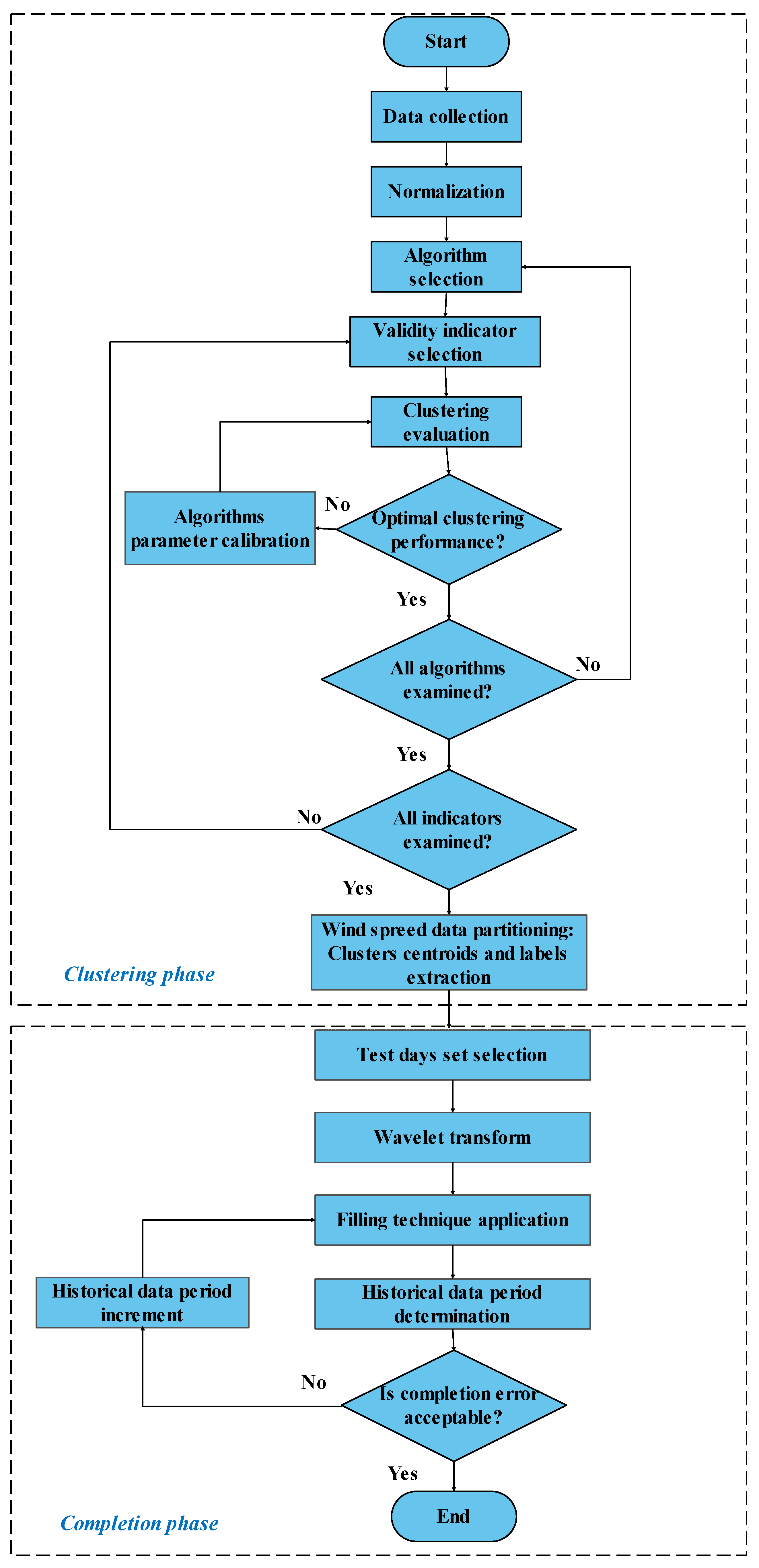
2.6. Proposed Methodology for Filling Missing Data for Days with Complete Absence of Data

The flow-chart of the methodology of missing data filling is depicted in Figure 2. It consists of the two main stages, namely the clustering and the completion stages. The daily wind speed series are decomposed using the discrete wavelet transform (DWT). Then, the clustering is applied separately on each wavelet component.
The volatility of the wind speed series is dealt with the Discrete Wavelet Transform (DWT); this transform is used to split up the original series into one low-frequency and some high-frequency subseries in the wavelet domain [43]. These subseries present a better behavior set compared to the original signal and thus, they can aid the performance of the clustering process. DWT provides a filter to the original series. The wavelet transforms are distinguished in Continuous Wavelet Transform (CWT) and DWT. Let f ( x ) and Φ ( x ) be the original series and a mother wavelet, respectively. The CWT W ( a , b ) of f ( x ) is expressed as [44]:
W ( a , b ) = 1 a + f ( x ) Φ ( x b a ) d x
where, the scale parameter a controls the spread of the wavelet, and the translation factor b determines its central position. The wavelet representation of f ( x ) with respect to the mother wavelet Φ ( x ) refers to the set of all wavelet coefficients W ( a , b ) . The wavelet coefficients W ( a , b ) in (6) represent how well the original signal f ( x ) and the mother wavelet match. The set of all wavelet coefficients W ( a , b ) associated to a particular signal, is the wavelet representation of the signal with respect to the mother wavelet. The CWT is accomplished by continuously scaling and translating the mother wavelet. But this concept may lead to increased redundant information. An alternative to this, is to consider certain scale, an approach known as DWT. In the DWT, each coefficient W ( m , n ) is expressed as [44]:
W ( m , n ) = 2 ( m 2 ) t = 0 T 1 f ( t ) Φ ( t n 2 m 2 m )
where T is the length of the signal f ( t ) and t is the discrete time index. A fast DWT has been proposed in [44]. The scaling and translation parameters are functions of the integer variables m and n ( a = 2 m and b = n 2 m ).
The DWT consists of four filters: decomposition low-pass, decomposition high-pass, reconstruction low-pass, and reconstruction high-pass filters. This approach leads to approximation (which is the low-frequency representation) and details (the difference between the high-frequency representations) of the original series. The original series is split by successive decompositions into lower resolution components. The process is shown in Figure 3. The original series is the sum of the low-frequency component A3 and the high-frequency components D1, D2, D3, i.e., f = A 3 + D 1 + D 2 + D 3 . In our paper, the wavelet function of type Daubencies of order 4 serves as the mother wavelet.
After the decomposition of the wind speed series, one clustering algorithm is selected and applied separately in the four components. The algorithm is executed for a variable number of clusters and their performance is checked by the validity indicators. In this clustering application we are interested in the clustering label of each day of the data set. Recall that in the present data set there are 106 days with complete absence of wind speed measurements. In order to validate the proposed methodology, days with complete data are extracted from the data set to serve as test days. Specifically, 31 days (i.e., two or three days from every month) are selected as test days. The clustering is applied to the rest of the days with no missing data, i.e., 203 days. A description of the method is presented below:
Step1. Set the number of clusters to k. Application of clustering in each component set of the 203 days. The clustering labels of the 203 days are obtained.
Step2. Let n be the number of the day that is missing from the data set. Extract the sequence S of l previous days, i.e., from day n and backwards. This sequence is denoted as:
S l n = { n i l + 1 , n i l + 2 , ... , n i 1 , n i }
We obtain a separate sequence for each wavelet component D1, D2, D3 and A3.
Step3. Conduct a correlation analysis in order to determine the correlation between the current day and the previous days. The results are shown in Figure 4. It can be observed that the current day is more correlated with the two previous days. The same conclusion is valid for the wavelet components.
Step4. According to the correlation analysis of Step3, we select l = 2. Search in the whole data set of the same sequences of clusters labels that are similar to the one of the same days.
Step5. Let r be the number of sequences that are similar to those of test day l. Also, we denote as the days with the same sequence similarity. Next, we calculate the Euclidean distances between day n + 1 and all the n r + 1 . Note that day n + 1 is the next day of the test day n and it is known. We keep the smaller Euclidean distance, i.e., min { d E u c l ( n + 1 , n r + 1 ) } . Then we use the day n r that corresponds to min { d E u c l ( n + 1 , n r + 1 ) } to fill the missing day n. To clarify this step, we present an illustrative example in Figure 5.
In this example, the test day is denoted as n. The two previous days belong to the 5th and 4th cluster, respectively. Therefore, we search for sequence {4,5} in the whole set. Suppose that two similar sequences found. The next step refers to calculation of Euclidean distance between days n + 1 and n 1 + 1 , and between days n + 1 and n 2 + 1 . Let the smaller distance corresponds to n 2 + 1 . Next we use the data of n 2 to fill the test day n.
Step6. Application of the inverse DWT to obtain the original wind speed series.
Step7. Calculate the mean absolute range normalized error (MARNE) between days n and n r [45]:
MARNE = 1 M m = 1 M | p m a p m f | max ( p m a ) × 100
where p m a and p m f are the actual and filled wind speed curve of the l-th day, respectively. MARNE is a percentage error metric. The dominator involves the maximum value of a data set; this approach eliminates the effect of obtaining extremely high values when the dominator receives values close to zero.
Step8. If MARNE is acceptable, terminate the process. Otherwise, increase the number of clusters to k + 1 and repeat Step1 to Step8.

2.7. Proposed Methodology for Filling Incomplete Data for Days with Partial Absence of Data
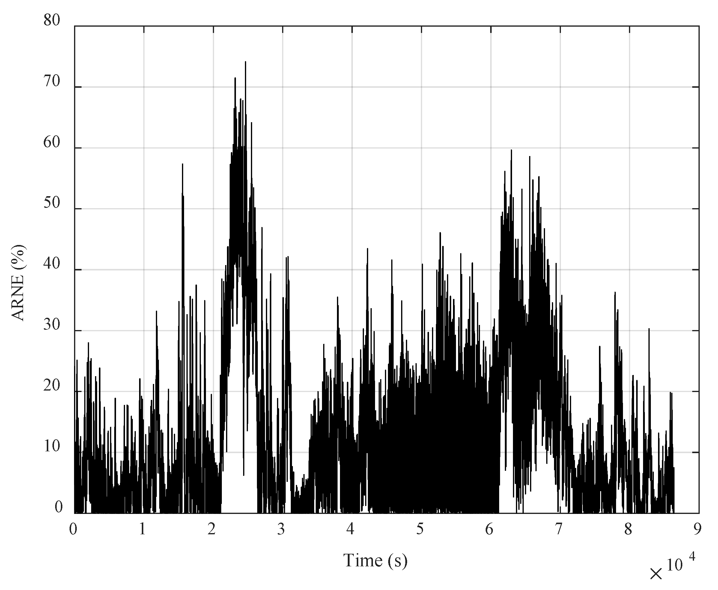
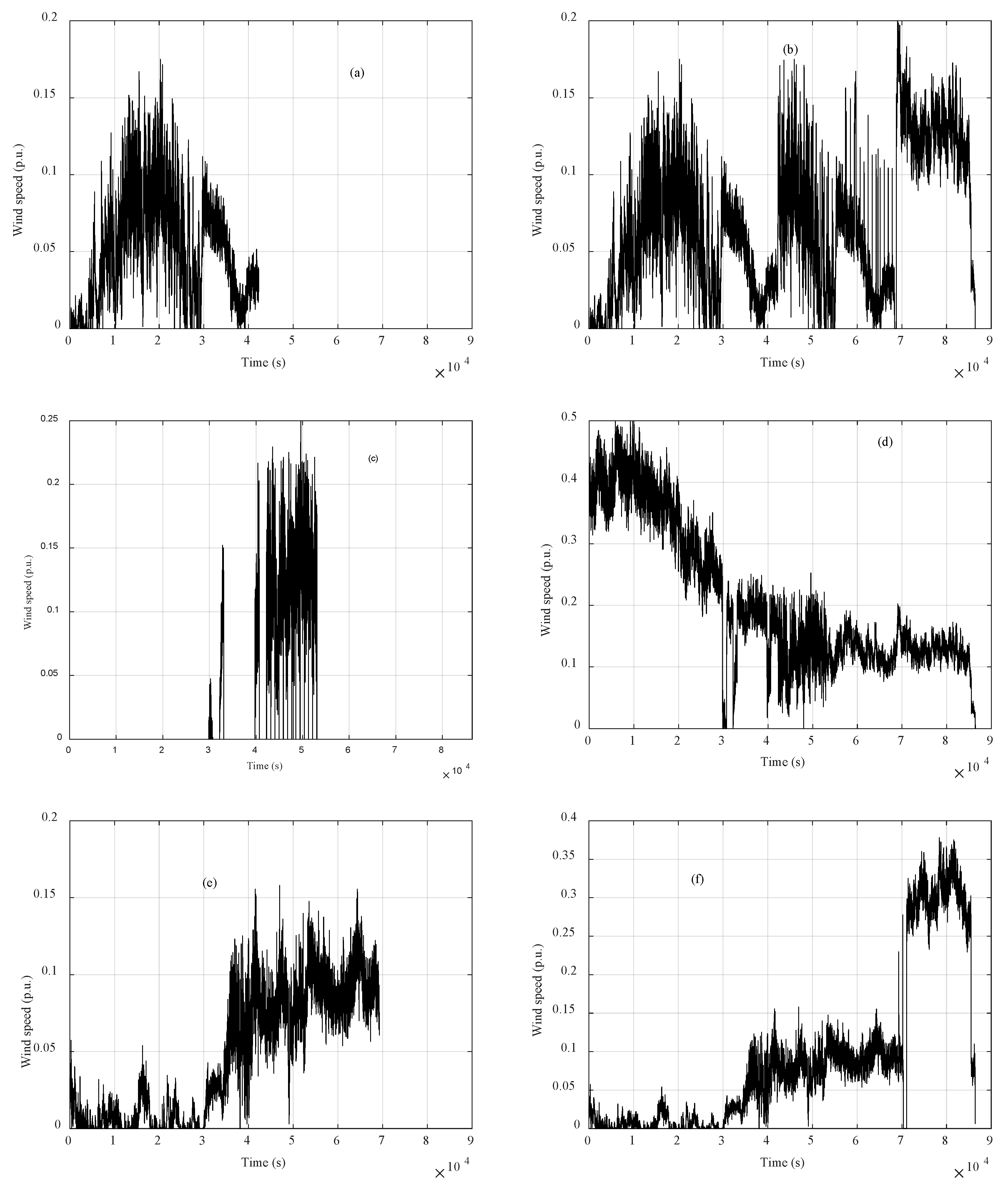
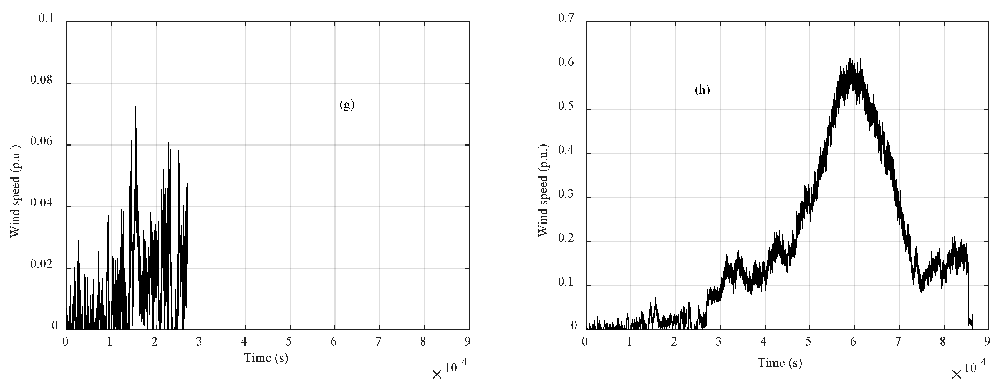
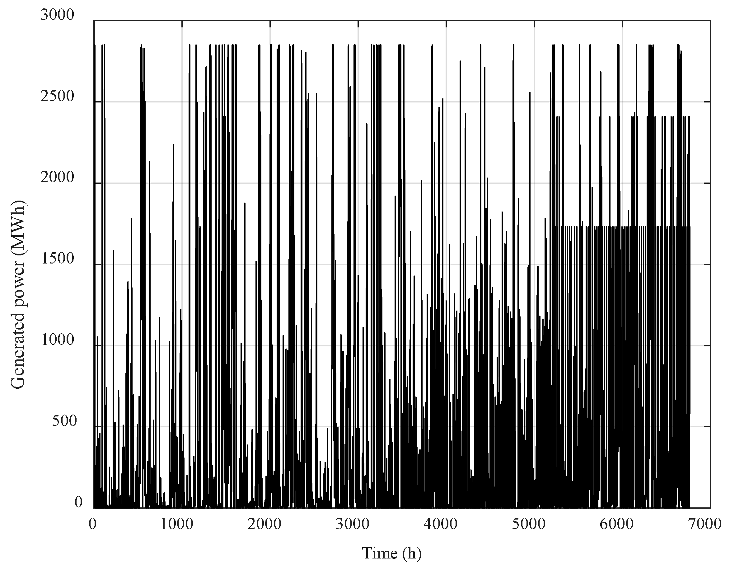
The incomplete days refer to days on which a number of measurements are absent during the day. Usually, the incomplete periods differ from day to day. Also, the number of missing data between the days is different. In order to fill those periods with measurements, Figure 6 presents two examples of days with incomplete data. After the preliminary dimensionality reduction described in Section 2, the complete days are represented with vector with D = 86400, i.e., each value corresponds to wind speed value per second. The days with incomplete data correspond to D < 86400.
The method for the incomplete data filling is analyzed in the following steps:
Step1. Set the number of clusters to k. Application of clustering in the 203 days. The clusters centroid (i.e., the normalized wind speed profiles) days are drawn.
Step2. Normalize the incomplete data set using Equation (1).
Step3. Compare each day with incomplete data with the k centroids using the Euclidean distance. In order to make the comparison feasible, the dimension of the k centroids is reduced to the number that corresponds to the one of each specific day.
Step4. Select the centroid that corresponds to the smaller Euclidean distance, i.e., the highest similarity.
Step5. Fill the missing values with the corresponding values of the selecting centroid.

3. Results

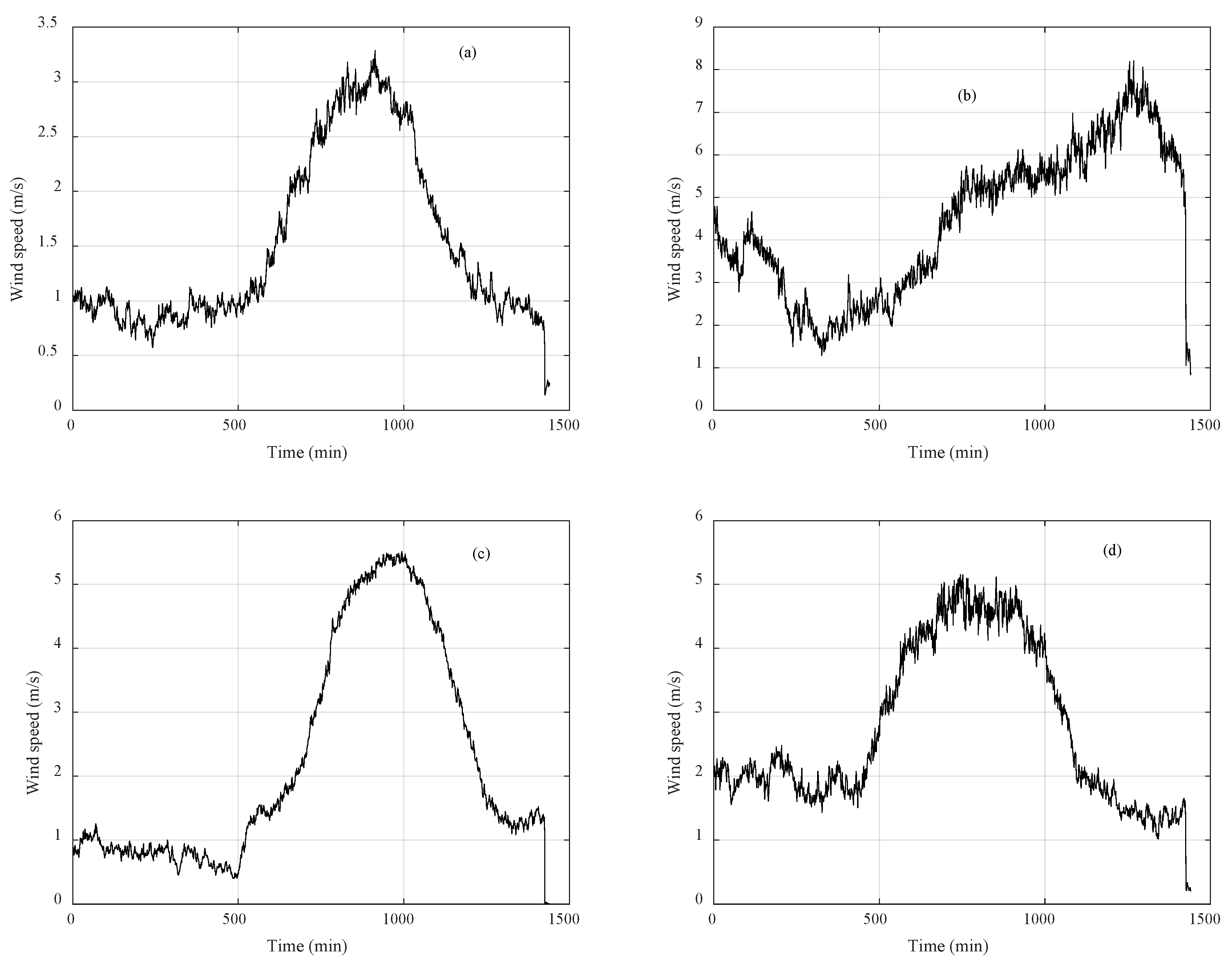
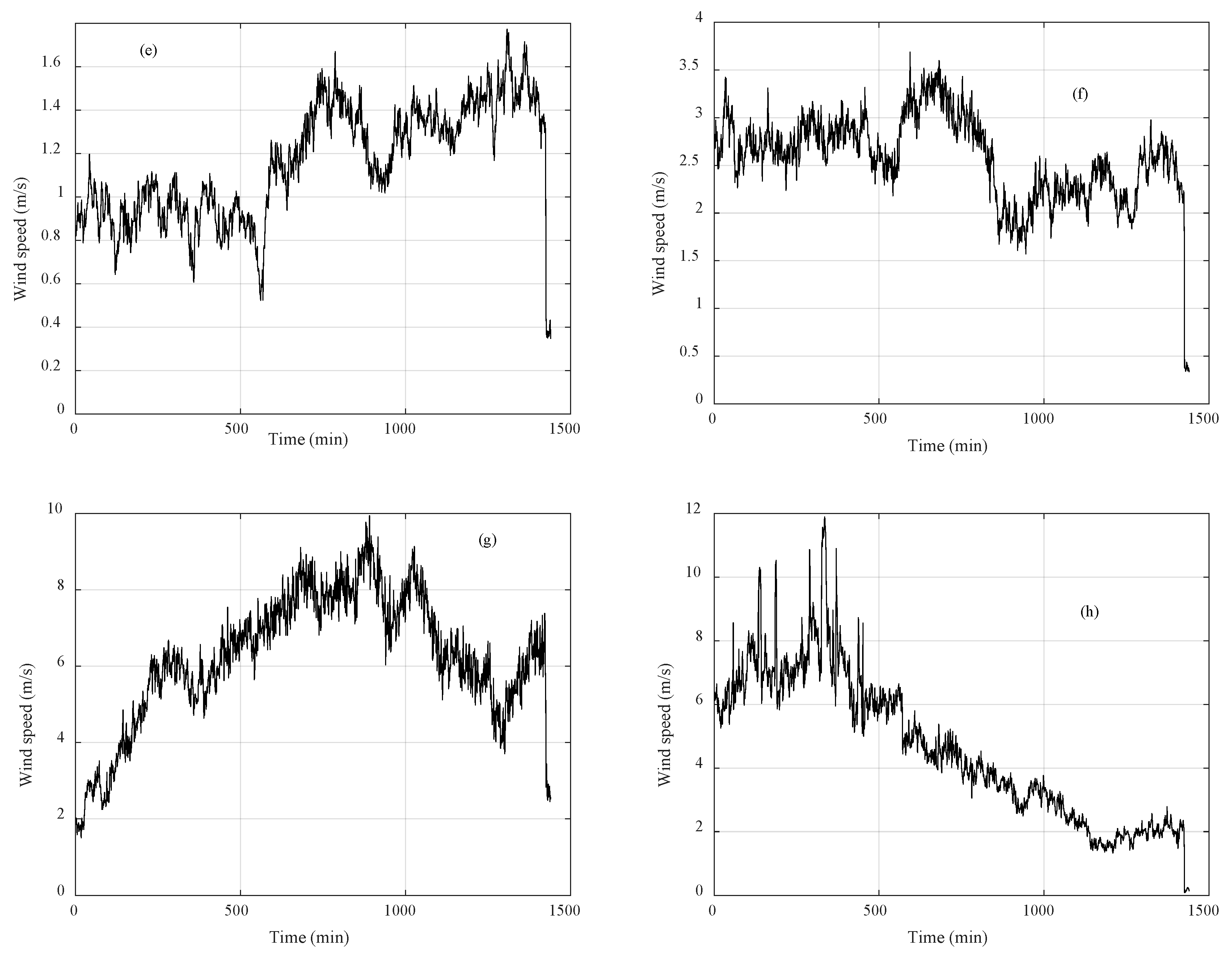
3.1. Clustering Algorithms Comparison and Wind Speed Profiles

The algorithms differ in terms of execution speed, input parameters requirements and others. A comparative analysis of common algorithms provides the basis for the systematic procedure to group together measurements with similar characteristics. The algorithms are tested on the 234 days with complete data. For the purpose of lowering the complexity of the problem, we transformed the patterns into per minute (D = 1140) and per hour (D = 24) time frames. However, as it will be further shown by the results, similar conclusions are drawn from the comparison of the algorithms if the initial set (D = 86400) is used. Each algorithm is separately applied to the two data sets for a variable number of clusters. There is no a priori information about the possible classes of the specific data. Hence, the clustering problem is purely data driven. This implies that the algorithms will produce results led by the existing similarities between the patterns. The number of clusters is unknown and therefore a series of experiments should take place. Each algorithm is applied for a variable number of clusters, and for every number, the values of the validity indicators are checked. We selected the number of clusters to vary from 2 to 30. To further improve the clustering credibility, a trial-and-error set of experiments should be conducted. These refer to a parametric analysis regarding the proper setting of the algorithm’s parameters. Regarding the K-means, the parameters that need to be determined are the maximum number of iterations and the minimum amount of improvement of the objective function between two successive iteration. The maximum number of iterations is set to 500 and the minimum improvement to 10 6 . The UPGMC is less complex; it needs only the merging stopping criterion between the consecutive merges. Actually, the merging stopping criterion is the number of the clusters that need to be set by the user. FCM needs the same parameters with K-means plus the value of the exponential parameter which controls the fuzziness of membership of each pattern to the clusters. For comparison, the same values with the K-means are selected. After a series of simulation, the fuzziness parameter is set equal to 2.70. The parameters of the SOM are: type of the map (i.e., one or two dimensions), training epochs, initial weights selection, initial neighborhood size and initial learning rate. Moreover, we consider one dimension maps, i.e., {1, K}, where K is the number of clusters. The training epochs equals to 500 and the initial weights are set to random values. Finally, the initial neighborhood size is set equal to two and the initial learning rate is set equal to 0.10. The comparisons of the algorithms considering the per minute and per hour representations are presented in Figure 7 and Figure 8, respectively.
The J indicator is a measure of cluster compactness. Low values of J refer to clusters that the majority of the patterns are distributed close to the centroid in the D-dimensioned patterns space. As the number of cluster increases, the Euclidean distance between the patterns and the centroids is lowering. K-means and SOM algorithms result in similar performance. The superiority of one algorithm over the others is demonstrated when leading to lower values for the majority number of simulations, i.e., number of clusters. According to J indicator, K-means wins the competition. Using the DBI measure, the UPGMC algorithm in both cases has a distinguished performance. The FCM leads to poor clustering and the K-means and SOM algorithm again have similar operation. The DBI curve has a volatile shape while the number of clusters varies. Again, the hierarchical algorithm UPGMC wins the competition when the clustering is evaluated with the SI measure in both data sets. According to the above analysis, reaching into a safe conclusion about the selection of the algorithm is a relatively difficult task. For instance, the UPGMC algorithm is not suitable for the data sets under study according to the J indicator. However, this is not the case when utilizing the DBI and SI indicators. Consequently, a set of validity indicators should be considered to reach safe conclusions about the algorithm proper selection.
To further explore the algorithms capabilities, the required execution time for clustering the data set with D = 1440 is measured. Table 1 shows the required time for 2 to 30 clusters as measured in a 2.20 GHz Pentium® B960 Dual Core™ with 8GB RAM 64-bit system. The third column shows the ratio with respect to the K-means. The importance of execution time will be more distinct in data sets characterized as “Big Data”. According to [46], an appropriate clustering algorithm for Big Data applications should satisfy the “3Vs” criterion, namely volume, variety and velocity. Volume refers to the ability of a clustering algorithm to deal with a large amount of data. Variety refers to the ability of a clustering algorithm to handle different types of data (numerical, categorical and others). Finally, velocity refers to the speed of a clustering algorithm on the Big Data. While offshore wind park installations are continually expanding, the need for collection, warehousing and processing of wind speed data is higher. The velocity of a clustering algorithm is important in big wind speed data sets. According to Figure 7 and Figure 8 and Table 1, the selection of the UPGMC is proposed.
Due to their shape, J and SI indicators can be used to decide the optimal number of clusters by employing the “knee” point detection method [47]. Regarding the J curve of Figure 8 corresponding to K-means, the optimal number of clusters is 9. Thus, the 234 patterns with wind speed values per second are optimally clustered in 9 clusters. Figure 9 displays the wind speed of the set with D = 1440 and the resulting 8 profiles are depicted in Figure 10. As it can be noticed for the figure, there is a variety of wind speed levels. The diversity of wind speed profiles indicate that the present data set include series that are volatile. Table 2 registers the day type distribution of the 8 clusters. The most populated clusters are #1 and #5 while #7 is the less populated. The #7 profile displays many peaks. Most of the Clusters include days from different seasons of the year. For instance, Cluster#5 contains days from all seasons and almost same number of days from the different months. Moreover Cluster#2 mostly contains fall and winter days and its profile peak is obtained during late evening hours.
For comparison reasons, Figure 11 shows the profiles that are generated by the UPGMC algorithm. Table 3 presents the clusters membership. The inherent operational aspect of UPGMC is it tendency to isolate atypical patterns. This approach of the UPGMC on clustering is useful in applications where the outliers and non-regular data need to be removed from the set and examined separately. According to Table 3 singleton clusters are produced. Particularly, one day of September 2012, one day of July 2013 and two days of August 2013 are treated as atypical patterns. Profile #7 shows quite dissimilar shape from the rest. The wind speed exhibits an increasing trend during that day. This day has been included in Cluster#1 by the K-means algorithm. Also, Profile#8 has a noticeable shape. There are many high peaks during the first morning hours. Afterwards, the wind speed follows to nearly zero levels. The day of Cluster#8 has been included in Cluster#8 by considering the K-means.

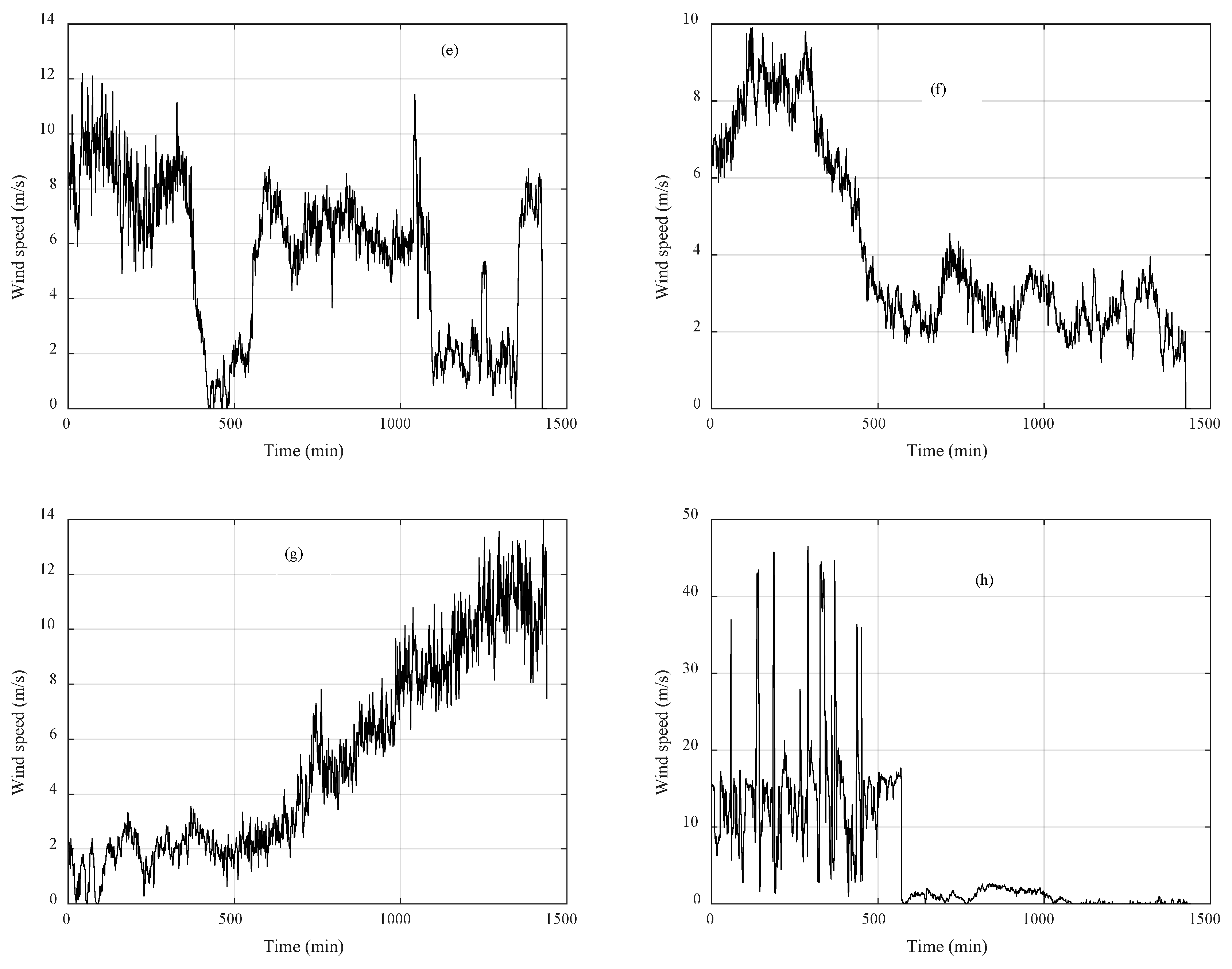
3.2. Missing Data Completion

In order to evaluate and examine the efficiency of the proposed method, an initial data set with D = 86,400 is involved and examined. K-means and UPGMC algorithms are used in order to cluster the set of the remaining 203 days. Recall that 31 days distributed across the year serve as the test to verify the proposed method. The algorithms are applied separately in the 4 sets corresponding to the D1, D2, D3 and A3 wavelet components. Every wavelet component set corresponds to 203 days. The algorithms are executed for 2 to 30 clusters. Using K-means algorithm and the J indicator, the optimal number of clusters equals to five. This number is kept for each component. The clustering labels are drawn and for each test day a specific sequence label of length equal to two is searched in the whole set. Note that this sequence label may differ among the components. For instance, the test day 09/02/2013 has the following sequences for the D1, D2, D3 and A3 components, respectively: {5,5}, {2,2}, {2,2} and {3,2}. When the matched sequences are obtained per component, the patterns that are selected to fill the missing day are summed to obtain the original wind speed series. Note that the selected days per wavelet component may differ. This signifies that the missing day completion can be done using a day that is obtained by the sum of different day components. Hence, this day is not an actual day of the set, but an artificial series derived from the sum of the wavelet components that correspond to different actual days.
As K-means and UPGMC are two different types of algorithm, their results on data partitioning are at least theoretically expected to differ. This is shown in Figure 7 and Figure 8. Table 4 presents the MARNEs per test day using the two algorithms. As it can be observed, UPGMC leads to lower errors as measured by the MARNE indicator. The last column of the Table presents the improvement that is achieved with the UPGMC over the K-means. According to the results as presented in Table 2, the K-means produces clusters with many members. Contrary to the UPGMC, K-means cannot isolate atypical patterns. This is the case with the UPGMC, as shown in Table 3. This is also observed in the results of the missing data completion method. The UPGMC isolates the atypical patterns found in the sets of D1, D2, D3 and A3 components. Then using the Euclidean distance metric, a search is held to identify the most similar pattern with one of day n + 1. Most patterns belong to the same cluster as it again can be observed in Table 3. Therefore, the search space, i.e., the population of available patterns is larger. Similarly, the number of pattern sequence matches is increased. According to this concept, the increment of the search space proportionally increases the possibility to find a more similar pattern with the test day n + 1. Considering the A3 component, the UPGMC creates a cluster with 221 members with label “1”, a cluster with five members with label “2”, two singletons clusters with labels “3” and “5” and a cluster with six members with label “4”. The vast majority of the patterns are gathered in cluster 1. The labels distribution of the K-means is: 49 members in cluster 1, 9 members in cluster 2, 55 members in cluster 3, 15 members in cluster 4 and 106 members in cluster 5. It can be concluded, that the number and types of days differ in the outputs of the two algorithms.
According to the findings of Table 4, the UPGMC leads to improvements that range between 0.05% and 62.28%, and an average value equal to 22.17%. For the case of day 09/10/2012 the two algorithms lead to the same results. Nearly identical results are met in the days 09/03/2013 and 01/04/2013, where the improvement rate is below 1%. Among the 31 days, the improvement is higher than 10% in 19 days. Also, it cannot be observed a distinctive improvement rate tendency among the seasons. High rates are met in December 2012, February 2013, March 2013, May 2013 and July 2013. The UPGMC results in MARNEs that are between 9.14% and 36.37%, with an average that equals to 16.85%, while the K-means results in MARNEs that are between 10.50% and 47.46%, with an average that equals to 22.41%. The lowest MARNE of the UPGMC is met at 15/07/2013. While the lowest MARNE of the K-means is also met at the same test day. The graphical comparison of the two algorithms is presented in Figure 12 and Figure 13. The figures show the completed and the actual series of several test days. The vertical axis is expressed in per unit (p.u) values. The horizontal axis refers to the time expressed in seconds. The test days are selected in a way to refer to different seasons.
It can be noticed that in the majority of the days the UPGMC generates series that follow the trends of the actual series. This is also the case with the K-means algorithm but in a smaller degree. For example, in Figure 12a the series that are obtained in most periods of the day follow the trends of the actual series.
Figure 14 shows the absolute range normalized error (ARNE) per second of the day 01/10/2012. The mean value of the error values corresponds to the MARNE indicator. At the beginning the ARNE values range is below the 20% threshold. Next, the errors are increasing. The sudden peak of 74.12% is met on the second 24,644 which is close to 07:00 AM. Totally, there are seven instances with errors higher than 70% that are met nearly close to the specific hour. For the next morning and noon hours the ARNE curve is relatively smooth. Again, low errors are met at night hours. Furthermore, the UPGMC results in series that follow the general trend of the actual one in days 01/02/2013, 23/04/2016, 09/06/2013 and 15/07/2013. Especially for 15/07/2013, the algorithm leads to a lower MARNE.

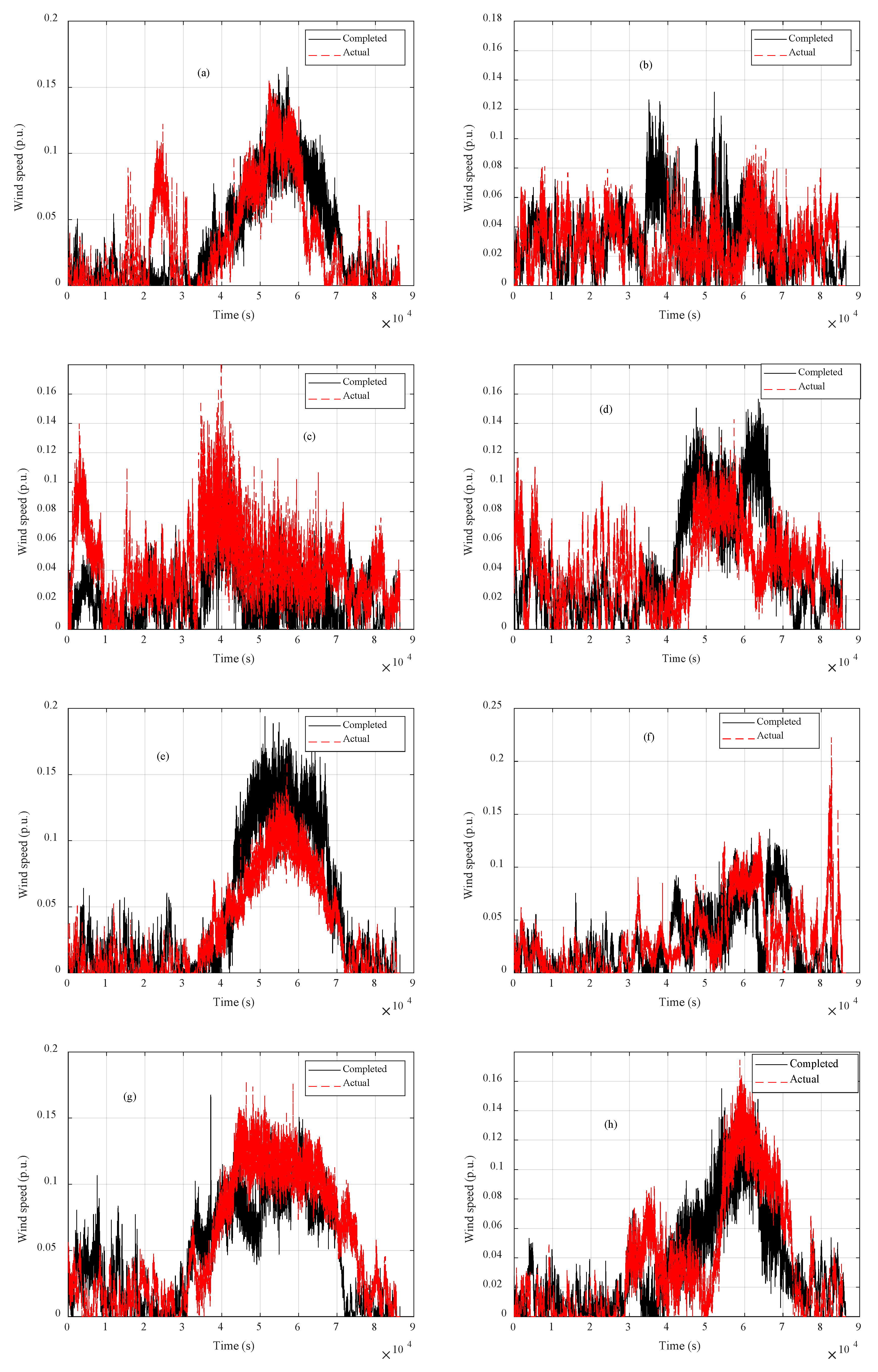
3.3. Incomplete Data Completion

The incomplete data completion refers to the filling of the days with sporadic measurements. This approach strengthens the assessment of the energy potential for the given region. Thus, the method developed for this set of simulations is a supporting stage to the energy potential evaluation part. By increasing the amount of data, the assessment becomes more robust. Hence, instead of using only the days with full data, by filling the incomplete days, the available data set for the assessment is increased. Figure 15 presents some of the findings of the present Section. More specifically, the original series of 01/11/2013, 01/12/2013, 19/06/2013 and 27/07/2013 are plotted together with the completed series.
The algorithm used for this example is the K-means. The Profile#6 is used for filling the day 01/11/2013. For this day the first 42293 wind speed values are available. By using the Euclidean distance, the incomplete series are compared with the profiles. Note that only the first 42293 values of the profiles are used for the purpose of making the similarity comparison feasible. The values until the last second are filled with those of Profile#6. Additionally, day 01/12/2013 is also filled with Profile#6; in this case, the first morning and late-night hours are used for the completion. Profile#2 is used for the day 19/06/2013. The SNMR system has collected the first 69285 wind speed values. Finally, Profile#1 is used for the summer day 27/07/2013. Here, only the first 27000 values are available. The incomplete series present high similarity with the respective first values of Profile#1 as it can be noticed in Figure 10. According to Table 2, Cluster#1 includes many summer days. The shape of the profile is relatively smooth with no sudden increments of wind velocity. The peak of Profile#1 is met on evening hours.
It should be noted that the proposed method can be used also for the rest measured environmental variables, i.e., temperature and wind direction. This is a different problem since the number of clusters may vary compared to the cluster number used for the speed values due to the different variations and degrees of volatility of the measured temperature and wind direction.
After the completion of the incomplete days, the final wind speed series can be used for several different applications (e.g., short-term energy assessment, preventive maintenance methods, monitoring tools). As a use case example and by interpolating the generated complete wind speed series to the power curve of a wind turbine, the expected short-term generated power is calculated for the period that the data refer to. For the case of the Vestas V112-3MW Offshore wind turbine with Cut-in speed, Cut-out speed and Nominal speed equal to 3 m/s, 25 m/s and 12 m/s, respectively, the calculated annual generated power equals to 3055 ΜWh [48].
In order to calculate the generated annual power, we need to calculate the wind speed v ( H ) at height H which is the height of the shaft of the wind turbine:
v ( H ) = v ( h ) ( H h ) a
where v ( h ) is the wind speed at height h = 3 m where the measurement took place (SNMR system) and a is a constant [49]. For the location under consideration is a = 0.10 . Moreover in our case H equals to 80 m. The interpolation is held via a first order polynomial. Based on the measured data the wind turbine generates power for 6766 h, i.e., for the 81.01% of the period that the wind speed data refer to. The hourly generated power series of the selected wind turbine is shown in Figure 16.
It should be noted that for the wind energy potential assessment of an offshore site long-term field measurements or satellite data (e.g., MERRA-2) should be used. Moreover, wake effects should be considered appropriately and accounted for the wind farm site design and for the identification of its layout. Also, a turbine type must be selected based on a techno-economical assessment (e.g., LCOE). The present paper deals with a developed novel method for filling missing wind data that can be used by different methods (e.g., the energy assessment of offshore wind turbines).

4. Discussion

Offshore wind turbine installations are continually gathering research interest since they are considered an efficient mechanism for covering the electrical needs of various isolated loads. The assessment of the energy potential of offshore wind turbines is a key factor that defines their successful implementation, operation and commercialization. The data used refer to many variables, the most being wind speed. However, due to metering failures or other factors the data may not present homogeneity due to incomplete or missing entries. This fact can lead to considerable limitations in the energy potential assessment and further, in the design of offshore wind parks. The present study focuses on the handling of incomplete data. A comparative analysis of clustering algorithms took place for grouping the daily wind speed curves. Each group is characterized by a typical curve. Through the typical curves, a descriptive model of the data is drawn. The main conclusions drawn from the algorithm’s application can be summarized in the following:
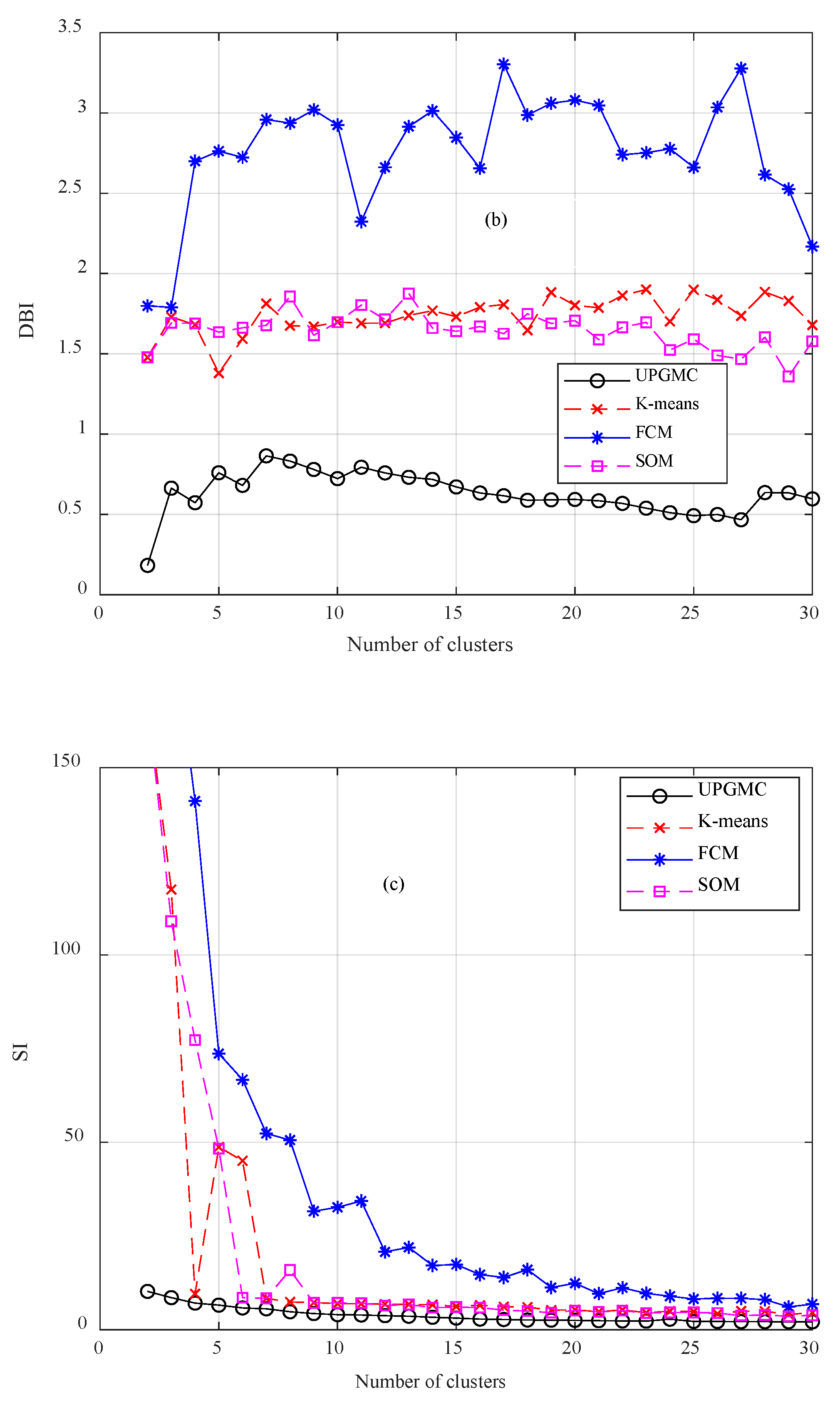
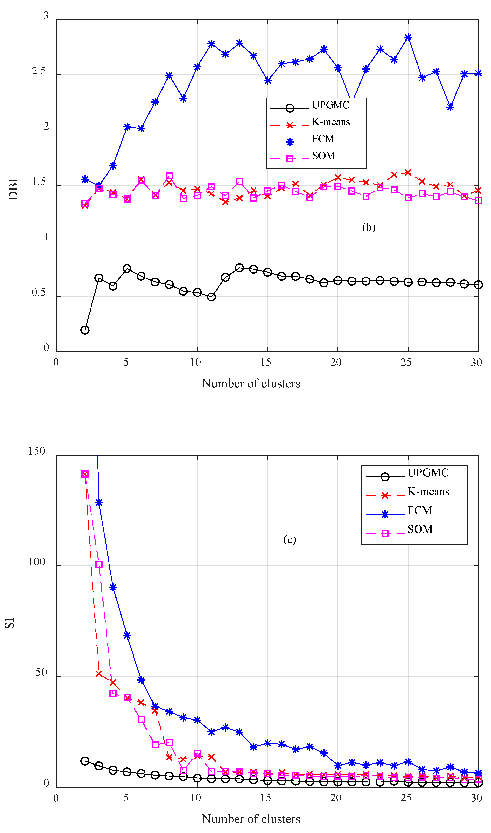
  • A set of validity indicators is required for determining the optimal algorithm. Clustering is application driven. Therefore, there is no universally acclaimed algorithm for all clustering problems.
  • The comparative analysis indicates that UPGMC is more appropriate for wind speed data clustering; FCM and SOM correspond to poor performance.
  • With respect to execution time, UPGMC requires the less time. SOM corresponds to high execution time and its utilization is not recommended for the problem under study.
  • The indicator J and SI are appropriate for determining the optimal number of clusters. This number differs among the time scales (second, minute and hour) of wind speed time series.
    Clustering is the core of the missing data completion techniques. Regarding the completion of days with a complete absence of data, the main conclusions can be summarized in the following:
  • The K-means leads to increased errors in all days of the test set compared to the UPGMC.
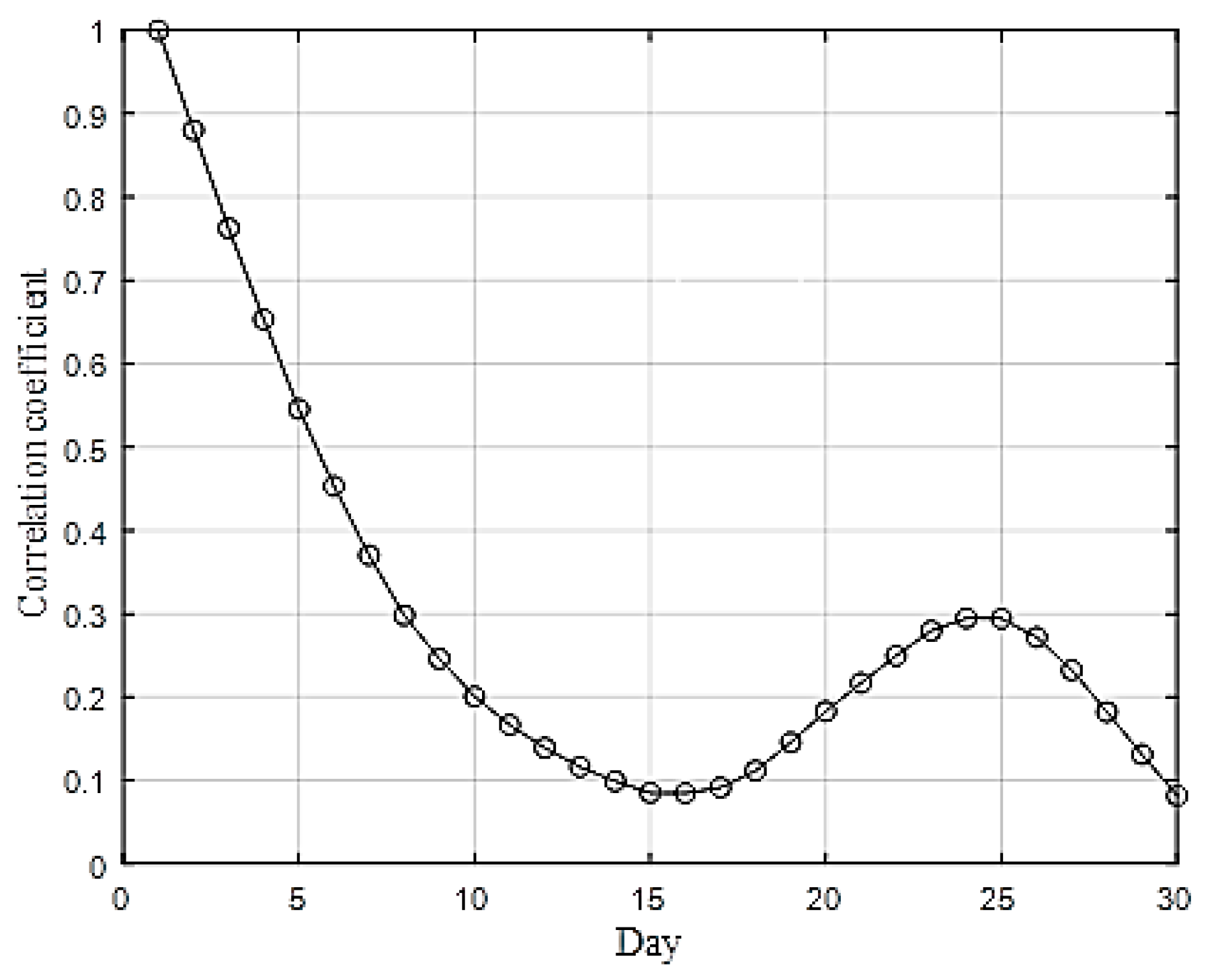
  • No strong correlation is observed between the seasonality of the day and the completion error.
Regarding the completion of the days with a partial absence of, the main conclusion is that for each day a dedicated comparison among the day and the wind speed profiles is needed. The number of missing elements of each day differs among the days. Accordingly, the dimension of wind speed profiles has to be reduced to fit the dimension of the incomplete day.
This paper contributes to the wind characteristics literature as presented below:
  • A set of various clustering algorithms have been compared for the analysis of the wind speed data. Contrary to the existing literature, the patterns for clustering refer to daily wind speed series. Apart from validity indicators, the algorithms have been checked in terms of complexity, i.e., the required execution time.
  • Two novel techniques of missing data filling have been proposed.
    The analysis of the present paper can be expanded to the following areas:
  • Examination of other clustering algorithms for the problem under study.
  • Development of new algorithms (i.e., multi-objective optimization) that aim to satisfy two criteria, for example the distances between patterns in the same cluster and the distances between the centroids among the clusters.
  • The utilization of new indicators for algorithm assessment, both for measuring the clustering error and complexity.
  • Examination of other mother wavelets of the DWT.
  • Implementation of the proposed missing data filling techniques in the variables that are related to the structural health monitoring of offshore installations.
Apart from the energy potential assessment, the missing data filling concept can be regarded in the wind layout farm optimization problem. As the quality of the wind speed patterns holds a critical role with respect to this problem, the scope is to implement the clustering and the missing data methods to derive more accurate wind speed time series by restoring the information lost due to missing values and track periodicities, trends and outliers, through clustering.
Incomplete and missing data provide many limitations for data exploitation. Therefore, a contemporary research topic is the examination of methods to deal with this case. Reduced information on wind speed patterns due to incomplete and missing data lead to challenges in the utilization of WTs and more specifically, in economic dispatch, unit commitment, WT sizing and wind farm layout optimization, generated electricity estimation and forecasting, and the management of the technical risks associated with the integration of WTs in power grids among others. Therefore, generator companies, system operators, regulatory authorities, WT equipment manufacturers and retailers can benefit from the methods presented in the paper. In order to lead to accurate results and information retrieval, data that cover more than one complete year are required. This is due to the need for examining potential trends, seasonalities, cyclic patterns and others. No data transformation or other processing are needed. Apart from wind speed profile extraction, clustering can provide outlier and other abnormalities detection. It should be noted that the methods for data filling are based solely on clustering and do not require further analysis and modeling. Hence, they are comprehensive and easily implemented and applied. The configuration of the PC system used in this paper is discussed in Section 3.1, and in this system the execution time of two methods is less than 30 s. This means that the computational cost is not a prohibitive factor for modern day PC systems. All methods, both clustering and data filling, are implemented in Matlab™ software, and thus, if an interested party plans to adapt the paper’s methods, they need to obtain a commercial or academic license to adopt the Matlab™ software. However, all the clustering algorithms used in the paper are also available in freeware software and in many programming languages.

Author Contributions

I.P.P. performed the research and wrote the first draft of the paper. C.M and D.C.A. set the objectives of the research, provided guidance for the research and revised the paper.

Funding

This research received no external funding.

Conflicts of Interest

The authors declare no conflict of interest.

References

  1. International Energy Agency. Renewables Information 2016; IEA: Paris, France, 2016. [Google Scholar]
  2. Esteban, M.D.; Diez, J.J.; López, J.D.; Negro, V. Why offshore wind energy? Renew. Energy 2011, 36, 444–450. [Google Scholar] [CrossRef] [Green Version]
  3. Breton, S.M.; Moe, G. Status, plans and technologies for offshore wind turbines in Europe and North America. Renew. Energy 2009, 34, 646–654. [Google Scholar] [CrossRef]
  4. Bilgili, M.; Yasar, A.; Simsek, E. Offshore wind power development in Europe and its comparison with onshore counterpart. Renew. Sustain. Energy Rev. 2011, 15, 905–915. [Google Scholar] [CrossRef]
  5. Snyder, B.; Kaiser, M.J. Ecological and economic cost-benefit analysis of offshore wind energy. Renew. Energy 2009, 34, 1567–1578. [Google Scholar] [CrossRef]
  6. Karimirad, M.; Michailides, C. V-shaped semisubmersible offshore wind turbine: An alternative concept for offshore wind technology. Renew. Energy 2015, 83, 126–143. [Google Scholar] [CrossRef]
  7. Karimirad, M.; Michailides, C. V-shaped Semisubmersible Offshore Wind Turbine Subjected to Misaligned Wave and Wind. J. Renew. Sustain. Energy 2016, 8, 023305. [Google Scholar] [CrossRef]
  8. Michailides, C.; Gao, Z.; Moan, T. Experimental Study of the Functionality of a Semisubmersible Wind Turbine Combined with Flap-Type Wave Energy Converters. Renew. Energy 2016, 93, 675–690. [Google Scholar] [CrossRef]
  9. Michailides, C.; Gao, Z.; Moan, T. Experimental and numerical study of the response of the offshore combined wind/wave energy concept SFC in extreme environmental conditions. Mar. Struct. 2016, 50, 35–54. [Google Scholar] [CrossRef]
  10. Pérez-Collazo, C.; Greaves, D.; Iglesias, G. A review of combined wave and offshore wind energy. Renew. Sustain. Energy Rev. 2015, 42, 141–153. [Google Scholar] [CrossRef] [Green Version]
  11. Rodrigues, S.; Restrepo, C.; Kontos, E.; Teixeira Pinto, R.; Bauer, P. Trends of offshore wind projects. Sustain. Energy Rev. 2015, 49, 1114–1135. [Google Scholar] [CrossRef]
  12. Little, R.J.; Rubin, D.B. Statistical Analysis with Missing Data; John Wiley and Sons: New York, NY, USA, 1987. [Google Scholar]
  13. Batista, P.A.; Monard, M.C. An analysis of four missing data treatment methods for supervised learning. Appl. Artif. Intell. 2003, 17, 519–533. [Google Scholar] [CrossRef]
  14. Grzymala-Busse, J.W.; Goodwin, L.K. Handling missing attribute values in preterm birth data sets. In Lecture Notes in Computer Science: Volume 3642. Rough Sets, Fuzzy Sets, Data Mining, and Granular Computing (RSFDGrC 2005); Slezak, D., Yao, J., Peters, J.F., Ziarko, W., Hu, X., Eds.; Springer: Regina, Canada, 2005; p. 3420351. [Google Scholar]
  15. Li, D.; Deogun, J.; Spaulding, W.; Shuart, B. Towards missing data imputation: A study of fuzzy K-means clustering method. In Lecture Notes in Computer Science: Volume 3066. Rough Sets and Current Trends in Computing (RSCTC 2004); Tsumoto, S., Slowinski, R., Komorowski, J., Grzymala-Busse, J.W., Eds.; Springer: Uppsala, Sweden, 2004; p. 573579. [Google Scholar]
  16. Acuna, E.; Rodriguez, C. The treatment of missing values and its effect in the classifier accuracy. In Classification, Clustering and Data Mining Applications; Banks, D., House, L., McMorris, F.R., Arabie, P., Gaul, W., Eds.; Springer: Berlin/Heidelberg, Germany, 2004; pp. 639–648. [Google Scholar]
  17. Wong, A.K.C.; Chiu, D.K.Y. Synthesizing statistical knowledge from incomplete mixed-mode data. IEEE Trans. Pattern Anal. Mach. Intell. 1987, 9, 796–805. [Google Scholar] [CrossRef]
  18. Schneider, T. Analysis of incomplete climate data: Estimation of mean values and covariance matrices and imputation of missing values. J. Clim. 2001, 14, 853–871. [Google Scholar] [CrossRef]
  19. Feng, H.A.B.; Chen, G.C.; Yin, C.D.; Yang, B.B.; Chen, Y.E. A SVM regression based approach to filling in missing values. In Lecture Notes in Artificial Intelligence: Volume 3683. Knowledge-Based Intelligent Information and Engineering Systems (KES 2005); Khosla, R., Howlett, R.J., Jain, L.C., Eds.; Springer: Berlin/Heidelberg, Germany, 2005; pp. 581–587. [Google Scholar]
  20. Troyanskaya, O.; Cantor, M.; Sherlock, G.; Brown, P.; Hastie, T.; Tibshirani, R.; Botstein, D.; Altman, R.B. Missing value estimation methods for DNA microarrays. Bioinformatics 2001, 17, 520–525. [Google Scholar] [CrossRef] [Green Version]
  21. Oba, S.; Sato, M.; Takemasa, I.; Monden, M.; Matsubara, K.; Ishii, S. A Bayesian missing value estimation method for gene expression profile data. Bioinformatics 2003, 19, 2088–2096. [Google Scholar] [CrossRef] [Green Version]
  22. Luengo, J.; García, S.; Herrera, F. A study on the use of imputation methods for experimentation with Radial Basis Function Network classifiers handling missing attribute values: The good synergy between RBFNs and Event Covering method. Neural Netw. 2010, 23, 406–418. [Google Scholar] [CrossRef]
  23. Luengo, J.; García, S.; Herrera, F. On the choice of the best imputation methods for missing values considering three groups of classification methods. Knowl. Inf. Syst. 2012, 32, 77–108. [Google Scholar] [CrossRef]
  24. Stefanakos, S.N.; Athanassoulis, G.A. A unified methodology for the analysis, completion and simulation of nonstationary time series with missing values, with application to wave data. Appl. Ocean Res. 2001, 23, 207–220. [Google Scholar] [CrossRef]
  25. Nikolaidis, A.; Georgiou, G.C.; Hadjimitsis, D.; Akylas, E. Filling in Missing Sea-Surface Temperature Satellite Data Over the Eastern Mediterranean Sea Using the DINEOF Algorithm. Cent. Eur. J. Geosci. 2014, 6, 27–41. [Google Scholar] [CrossRef]
  26. Xu, R.; Wunsch, D. Clustering; John Wiley & Sons. Inc.: Hoboken, NJ, USA, 2006. [Google Scholar]
  27. Dar, K.M.; Javed, I.; Amjad, W.; Aslam, S.; Shamim, A. Survey of clustering applications. J. Netw. Commun. Emerg. Technol. 2015, 4, 10–14. [Google Scholar]
  28. Steinley, D. K-means clustering: A half-century synthesis. Br. J. Math. Stat. Psychol. 2006, 59, 1–34. [Google Scholar] [CrossRef]
  29. Fortuna, L. Clustering Daily Wind Speed Time Series. Book Chapter: Nonlinear Modeling of Solar Radiation and Wind Speed Time Series; Springer: Berlin/Heidelberg, Germany, June 2016; pp. 79–89. [Google Scholar]
  30. Ouyang, T.; Kusiak, A.; He, Y. Modeling wind-turbine power curve: A data partitioning and mining approach. Renew. Energy 2017, 102, 1–8. [Google Scholar] [CrossRef]
  31. Tamah Al-Shammari, E.; Shamshirband, S.; Petkovi, D.; Zalnezhad, E.; Yee, P.L.; Taher, R.S.; Cojba, Z. Comparative study of clustering methods for wake effect analysis in wind farm. Energy 2016, 95, 573–579. [Google Scholar] [CrossRef]
  32. Di Piazza, A.; Di Piazza, M.C.; Ragusa, A.; Vitale, G. Statistical processing of wind speed data for energy forecast and planning. In Proceedings of the International Conference on Renewable Energies and Power Quality, Granada, Spain, 23–25 March 2010; pp. 1417–1422. [Google Scholar]
  33. Sánchez-Pérez, P.A.; Robles, M.; Jaramill, O.A. Real time Markov chains: Wind states in anemometric data. J. Renew. Sustain. Energy 2016, 8, 023304. [Google Scholar] [CrossRef] [Green Version]
  34. Carreón-Sierra, S.; Salcido, A.; Castro, T.; Celada-Murillo, A.T. Cluster analysis of the wind events and seasonal wind circulation patterns in the Mexico city region. Atmosphere 2015, 6, 1006–1031. [Google Scholar] [CrossRef]
  35. Lorenzo, J.; Mendez, J.; Castrillon, M.; Hernandez, D. Short-Term Wind Power Based on Cluster Analysis and Artificial Neural Networks. Volume 6691 of the Series Lecture Notes in Computer Science; Springer: Berlin/Heidelberg, Germany, 2011; pp. 191–198. [Google Scholar]
  36. Esmaeili, M.A.; Twomey, J. Self-Organizing Map (SOM) in wind speed forecasting: A new approach in computational intelligence (CI) forecasting methods. In Proceedings of the ASME/ISCIE 2012 International Symposium on Flexible Automation, St. Louis, MO, USA, 18–20 June 2012; pp. 405–409. [Google Scholar]
  37. Michailides, C.; Loukogeorgaki, E.; Angelides, D.C. Monitoring the response of connected moored floating modules. In Proceedings of the Twenty-third International Offshore and Polar Engineering, Anchorage, AK, USA, 30 June–5 July 2013; pp. 869–876, ISBN 978-1-880653-99-9. [Google Scholar]
  38. Tseranidis, S.; Theodoridis, L.; Loukogeorgaki, E.; Angelides, D.C. Investigation of the condition and the behavior of a modular floating structure by harnessing monitoring data. Mar. Struct. 2016, 50, 224–242. [Google Scholar] [CrossRef]
  39. Chicco, G. Overview and performance assessment of the clustering methods for electrical load pattern. Energy 2012, 42, 68–80. [Google Scholar] [CrossRef]
  40. Greenlaw, R.; Kantabutra, S. Survey of clustering: Algorithms and applications. Int. J. Inf. Retr. Res. 2013, 3, 1–29. [Google Scholar] [CrossRef]
  41. Dharmarajan, A.; Velmurugan, T. Applications of partition based clustering algorithms: A survey. In Proceedings of the 2013 IEEE International Conference on Computational Intelligence and Computing Research, Tamilnadu, India, 26–28 December 2013; pp. 703–707. [Google Scholar]
  42. Neha, D.; Vidyavathi, B.M. A survey on applications of data mining using clustering techniques. Int. J. Comput. Appl. 2015, 126, 7–12. [Google Scholar]
  43. Mallat, S. A theory for multiresolution signal decomposition-the wavelet representation. IEEE Trans. Pattern Anal. Mach. Intell. 1989, 11, 674–693. [Google Scholar] [CrossRef]
  44. Amjady, N.; Keynia, F. Short-term load forecasting of power systems by combination of wavelet transform and neuro-evolutionary algorithm. Energy 2009, 34, 46–57. [Google Scholar] [CrossRef]
  45. Soldo, B.; Potocnik, P.; Simunovi, G.; Sari, T.; Govekar, E. Improving the residential natural gas consumption forecasting models by using solar radiation. Energy Build. 2014, 69, 498–506. [Google Scholar] [CrossRef]
  46. Fahad, A.; Alshatri, N.; Tari, Z.; Alamr, A.; Khalil, I.; Zomaya, A.Y.; Foufou, S.; Boura, A. A survey of clustering algorithms for Big Data: Taxonomy and empirical analysis. IEEE Trans. Emerg. Top. Comput. 2014, 3, 267–279. [Google Scholar] [CrossRef]
  47. Panapakidis, I.P.; Alexiadis, M.C.; Papagiannis, G.K. Deriving the optimal number of clusters in the electricity consumer segmentation procedure. In Proceedings of the 10th European Energy Market Conference (EEM13), Stockholm, Sweden, 27–31 May 2013; pp. 1–8. [Google Scholar]
  48. Vestas V112-3.0 MW. Available online: http://www.vestas.cz/ (accessed on 26 March 2019).
  49. Hsu, S.A.; Meindl, E.A.; Gilhouse, D.B. Determining the power-law wind-profile exponent under near-neutral stability conditions at sea. J. Appl. Meteorol. 1994, 33, 757–765. [Google Scholar] [CrossRef]
Figure 1. (a) Solar panels; (b) Industrial computer of SNMR; (c) Energy storage batteries; (d) Wind speed and wind direction sensor.
Electronics 08 00418 g001
Figure 2. Flow-chart of the methodology of missing data filling.
Electronics 08 00418 g002
Figure 3. Multi-level decomposition process.
Electronics 08 00418 g003
Figure 4. Correlation coefficient between current and previous days.
Electronics 08 00418 g004
Figure 5. Example of cluster label sequence.
Electronics 08 00418 g005
Figure 6. Examples of days with incomplete data: (a) 01/11/2013; (b) 01/12/2013.
Electronics 08 00418 g006
Figure 7. Algorithms comparison using: (a) J; (b) DBI; (c) SI indicators. The patterns dimension is D = 1440.
Electronics 08 00418 g007aElectronics 08 00418 g007b
Figure 8. Algorithms comparison using: (a) J; (b) DBI; (c) SI indicators. The patterns dimension is D = 24.
Electronics 08 00418 g008aElectronics 08 00418 g008b
Figure 9. Initial data set.
Electronics 08 00418 g009
Figure 10. Wind speed profiles after the application of the K-means algorithm: (a) Profile#1; (b) Profile#2; (c) Profile#3; (d) Profile#4; (e) Profile#5; (f) Profile#6; (g) Profile#7; (h) Profile#8.
Electronics 08 00418 g010aElectronics 08 00418 g010b
Figure 11. Wind speed profiles after the application of the UPGMC algorithm: (a) Profile#1; (b) Profile#2; (c) Profile#3; (d) Profile#4; (e) Profile#5; (f) Profile#6; (g) Profile#7; (h) Profile#8.
Electronics 08 00418 g011aElectronics 08 00418 g011b
Figure 12. Completed and actual data of: (a) 01/10/2012; (b) 09/11/2012; (c) 09/01/2013; (d) 01/02/2013; (e) 23/04/2016; (f) 16/05/2013; (g) 09/06/2013; (h) 15/07/2013. The clustering was held with the UPGMC algorithm.
Electronics 08 00418 g012
Figure 13. Completed and actual data of: (a) 01/10/2012; (b) 09/11/2012; (c) 09/01/2013; (d) 01/02/2013; (e) 23/04/2016; (f) 16/05/2013; (g) 09/06/2013; (h) 15/07/2013. The clustering was held with the K-means algorithm.
Electronics 08 00418 g013
Figure 14. Absolute Range Normalized Error (ARNE) per second of 01/10/2012.
Electronics 08 00418 g014
Figure 15. Examples of incomplete data filling: (a) Incomplete day 01/11/2013; (b) Completed day 01/11/2013; (c) Incomplete day 01/12/2013; (d) Completed day 01/12/2013; (e) Incomplete day 19/06/2013; (f) Completed day 19/06/2013; (g) Incomplete day 27/07/2013; (h) Completed day 27/07/2013.
Electronics 08 00418 g015aElectronics 08 00418 g015b
Figure 16. Hourly generated power of the wind turbine.
Electronics 08 00418 g016
Table 1. Required execution time for 2 to 30 clusters.
AlgorithmTime (s)Ratio
K-means33.241
UPGMC5.280.15
FCM282.498.49
SOM658.3119.80
Table 2. Number of days and day types per cluster. The clustering was held with the K-means algorithm.
ClusterNumber of Days Per ClustersGeneral Description of the Day Types
160Most days October 2012, six days of March 2013, most days of April 2013, six days of May 2013, six days of June 2013, three days of July 2013 and six days of August 2013
29One day per the following months: October 2012, December 2012, January 2013, May 2013 and June 203. Two days of the following moths: February 2013 and March 2013
341Two days of March 2013, five days of April 2013, most days of May 2013, June 2013 and July 2013
427Five days of October 2012, 3 days of November 2012, few days of February 2013 and March 2013, seven days of July 2013
551Eight days of October 2012, twelve days of November 2012, four days of December 2012, seven days of January 2013, five days of February 2013, eight days of March 2013, few days of April 2013, May 2013 and June 2013
628Five days of November 2012, few days of December 2012, January 2013 and February 2013, five days of March 2013, five days of May 2013
77Few days of December 2012 and March 2013
811Few days of February 2013 and May 2013, one day of August 2013
Table 3. Number of days and day types per cluster. The clustering was held with the UPGMC algorithm.
ClusterNumber of Days Per ClustersGeneral Description of the Day Types
11One day of September 2012
25Two days of September 2012, three days of October 2012
37Seven days of October 2012
4214All the rest days
51One day of July 2013
64Four days of August 2013
71One day of August 2013
81One day of August 2013
Table 4. Comparison of the K-means and the UPGMC algorithms in terms of missing data completion errors.
Day NumberDateMARNE (%)MARNE (%) Improvement
UPGMCK-means
101/10/201211.6415.2423.62
209/10/201214.0914.090
316/10/201213.9216.8417.33
401/11/201218.2518.441.03
509/11/201220.6425.1117.80
616/11/201219.8822.6812.34
701/12/201219.6722.3812.10
809/12/201217.2718.647.34
917/12/201216.5129.6144.24
1009/01/201312.3713.387.54
1116/01/201327.6730.108.07
1201/02/201318.0921.6616.48
1309/02/201317.9047.4662.28
1413/02/201319.4920.605.38
1501/03/201324.0624.742.74
1609/03/201319.5119.520.05
1716/03/201318.7939.1752.02
1801/04/201336.3736.670.81
1916/04/201316.6218.319.22
2023/04/201312.0319.8439.36
2101/05/201314.3528.6949.98
2209/05/201310.65 14.2625.31
2316/05/20139.9016.4739.89
2401/06/201318.89 27.7131.82
2509/06/201312.4821.0240.62
2616/06/201311.03 16.2131.95
2701/07/201317.0332.0146.79
2809/07/201314.0714.976.01
2915/07/20139.1410.5012.95
3001/08/201317.4618.334.74
3109/08/201312.8320.3436.92

