Abstract
In recent years, Transformer-based methods have demonstrated proficiency in capturing complex patterns for time series forecasting. However, their quadratic complexity relative to input sequence length poses a significant bottleneck for scalability and real-world deployment. Recently, the Mamba architecture has emerged as a compelling alternative by mitigating the prohibitive computational overhead and latency inherent in Transformers. Nevertheless, a vanilla Mamba backbone often struggles to adequately characterize intricate temporal dynamics, particularly long-term trend shifts and non-stationary behaviors. To bridge the gap between Mamba’s global scanning and local dependency modeling, we propose C-T-Mamba, a hybrid framework that synergistically integrates a Mamba block, channel attention, and a temporal convolution block. Specifically, the Mamba block is leveraged to capture long-range temporal dependencies with linear scaling, the channel attention mechanism filters redundant information, and the temporal convolution block extracts multi-scale local and global features. Extensive experiments on five public benchmarks demonstrate that C-T-Mamba consistently outperforms state-of-the-art (SOTA) baselines (e.g., PatchTST and iTransformer), achieving average reductions of 4.3–18.5% in MSE and 3.9–16.2% in MAE compared to representative Transformer-based and CNN-based models. Inference scaling analysis reveals that C-T-Mamba effectively breaks the computational bottleneck; at a horizon of 1536, it achieves an reduction in GPU memory and over 10× speedup compared to standard Transformers. At 2048 steps, its latency remains as low as 8.9 ms, demonstrating superior linear scaling. These results underscore that C-T-Mamba achieves SOTA accuracy while maintaining a minimal computational footprint, making it highly effective for long-term multivariate time series forecasting.
1. Introduction
Time series forecasting represents a significant research avenue within the domains of statistics and machine learning [1,2]. Its applications are pervasive, spanning a multitude of disciplines, including economics, finance, meteorology, energy, transportation, and healthcare. Time series data are observations of variables recorded in chronological order, and thus contain information about the historical evolution of the data, as well as future trends and changes. These can be predicted by analyzing and modeling the data [3]. An overview of typical time series data, specifically the Oil Temperature feature from the ETTm1 dataset, is illustrated in Figure 1. Currently, there are two main categories of time series prediction methods based on machine learning: (1) neural network models based on Transformer architecture, and (2) neural network models with non-Transformer architecture [4].
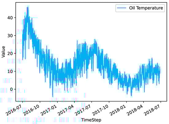
Figure 1.
Data overview of the Oil Temperature feature column in the ETTm1 dataset.
- Neural network models based on Transformer architecture:
The Transformer model was initially introduced to the field of Natural Language Processing (NLP), where it achieved considerable success [5]. This led to its adoption by researchers in the field of time series prediction. The self-attention mechanism enables the model to focus on all data points in the entire sequence simultaneously, thereby facilitating the capture of temporal dependencies and the learning of global patterns and overall trends in the sequence [6]. In comparison to traditional Recurrent Neural Network (RNN) [7] and Long Short-Term Memory (LSTM) [8] models, RNN is susceptible to the issue of gradient disappearance or gradient explosion when dealing with long time series data. Similarly, LSTM’s intricate gating mechanism and sequential processing characteristics result in a lack of computational efficiency, as evidenced by the persistence of the gradient problem observed in RNN. Transformer addresses these challenges through the integration of a self-attention mechanism and a feedforward network, thereby enhancing the stability and efficiency of the model training process. Nevertheless, self-attention enables Transformer to grasp the global context, but it also introduces the challenge of increased complexity. Self-attention necessitates calculating the correlation between each token in the input sequence and all other tokens, which involves significant time and space considerations. The complexity of this calculation is proportional to the square of the length of the input sequence. When the input sequence is of considerable length, the transformer model will consume a significant amount of computational resources and storage space, which may result in reduced efficiency and performance degradation. To address this challenge, subsequent research has proposed sparse attention methods, which reduce the number of correlation pairs computed in the self-attention mechanism, thereby reducing the time and space complexity. This enables the transformer model to process longer input sequences.
The ProbSparse attention mechanism in Informer [9] achieves in terms of time complexity and memory usage, which reduces the computational complexity from to by using the KL scattering method to evaluate the sparsity of the ith query and then selecting the TOP u query. The Autoformer [10] implements an effective autocorrelation mechanism to uncover dependencies and aggregate information at the sequence level. Its computational efficiency is characterized by a time complexity of . Through the application of the Wiener-Khinchin theorem and Fourier Transform, the auto-correlation method computes coefficients for sequences, subsequently establishing confidence levels for each cycle length. Following this analysis, the top k cycle lengths are prioritized for integration, thereby completing the extraction of temporal dependencies. The Reformer [11] replaces dot product attention with locally sensitive hashing, reducing the time complexity from to . FEDformer [12] proposes an attention mechanism that uses low-order frequency approximation and hybrid expert decomposition to control distributional bias. The proposed frequency-augmented structure separates the length of the input sequence from the dimension of the attention matrix, thus achieving linear complexity. The authors proved that the self-attention mechanism can be approximated by low-rank matrices, and further used this finding to propose a new self-attention mechanism that reduces the overall self-attention complexity in time and space from to . The Crossformer [13] is a time series forecasting model based on the Transformer architecture designed for multivariate time series (MTS) forecasting. In addition to the traditional cross-temporal dependencies, Crossformer incorporates cross-dimensional dependencies, thereby addressing one of the key issues often overlooked in existing Transformer models for MTS forecasting. The DSW embedding technique and the two-stage attention (TSA) layer enable Crossformer to effectively capture the complex relationships inherent in MTS data, thereby enhancing the accuracy of the forecasts produced.
- Neural network models with non-Transformer architecture:
FourierGNN [14] introduces a novel data structure, the hypervariable graph, which treats each sequence value as a graph node, collectively capturing spatio-temporal dynamics and transforming MTS predictions into predictions on the hypervariable graph. FourierGNN combines the Fourier Graph Operator (FGO), which performs matrix multiplications in the Fourier space, enhancing the expressive power and decreasing the complexity, thus enabling efficient prediction.
In order to adaptively discover multi-periodicity and extract complex temporal variations from the transformed 2D tensor, TimesNet [15] proposes the use of TimeBlock, which is a parameter-efficient initial block. The Multilayer Perceptron (MLP) is redesigned in the frequency domain with the objective of efficiently capturing the underlying patterns of time series with a global view and energy compression.
TiDE [16] proposes a multilayer perceptron (MLP)-based encoder-decoder model, the Time Series Dense Encoder (TiDE), for long-term time series forecasting. This model offers the simplicity and speed of a linear model while being able to handle covariates and nonlinear dependencies. Theoretically, the authors demonstrate that, under specific assumptions, the most straightforward linear simulation of TiDE model can achieve near-optimal error rates for linear dynamical systems (LDS).
State Space Model (SSM) [17] has demonstrated considerable potential for long-term dependency modeling and has achieved notable advancements in various domains of Artificial Intelligence (AI). However, it lacks the capability for dynamic inference, which led to the development of the Mamba model. Mamba addresses the computational inefficiency of Transformer on long sequences by integrating a selective state-space model that enables content-based inference and selective information propagation along the sequence length dimension, thereby providing rapid inference and linear scaling of sequence length. Unlike other models, the Mamba architecture does not rely on attention or MLP blocks. Mamba’s architecture is distinguished by selective information propagation and fast inference, as well as linear scaling of sequence length. Notably, it does not rely on attention or MLP blocks.
In this study, we present the Mamba model as a substitute for the Transformer framework. Our objective is to tackle the challenge of training scaling quadratically based on input sequence length. Additionally, we integrate the channel mixing attention module to capture intricate temporal changes within the sequence. Lastly, we employ temporal convolutional block for comprehensive global and local feature integration. This approach effectively harmonizes model complexity with performance.
The shift from traditional parametric models to architectures like C-T-Mamba is further motivated by the inherent risks of model misspecification. As demonstrated by the Hassani theorem, empirical correlation structures in time series often exhibit non-intuitive constraints that can undermine naive parametric inference [18]. By adopting a more flexible, SSM-based framework, C-T-Mamba avoids rigid distributional assumptions, providing more robust power in capturing non-stationary temporal dynamics. Overall, our main contributions are as follows:
- (1)
- We put forth a novel model, designated C-T-Mamba, which is based on the Mamba architectural framework. This approach effectively supplants the computationally expensive self-attention module in Transformer with the introduction of innovative channel mixing and temporal convolution block designs, thereby facilitating the discernment of intricate temporal patterns in time series.
- (2)
- Channel attention is employed to accentuate salient features within the sequence, while a temporal convolution block centered on deeply separable convolution is utilized to integrate the extracted features before capturing the global information and local features of the sequence.
- (3)
- Our model demonstrates superior performance compared to existing time series forecasting models on five public datasets of time series.
2. Related Work
2.1. Time Series Forecasting Tasks
Let us consider a time series, represented by the vector of values , In this context, the term denotes the time at which t of the observation occurs. The objective of time series forecasting is to employ the available historical observations to make predictions about future events . Mathematically, time series forecasting can be formalized as a function , which utilizes past observations to predict future observations .
2.2. Applications of Mamba
2.2.1. Mamba for Natural Language Processing
The Jamba [19] architecture represents a novel approach that combines the Attention and Mamba layers with the MoE module and its open implementation, achieving state-of-the-art performance while supporting long contexts. Jamba offers the largest model with 12 B active parameters and 52 B total available parameters, and is capable of supporting context lengths up to 256 K tokens, even when processing 140 K tokens of text. The Jamba model offers a maximum of 12 billion active parameters and 52 billion total available parameters, supporting context lengths up to 256,000 tokens, even when processing 140,000 tokens of text, on a single 80 GB GPU.
2.2.2. Applications of Mamba to Computer Vision
Mamba [20] proposes a novel two-branch network, designated as Remote Sensing Image Semantic Segmentation Mamba (Mamba), which has been specifically devised for remote sensing tasks. Mamba employs VSS modules to construct a secondary branch that furnishes supplementary global information to the convolution-based primary branch. Furthermore, in consideration of the disparate characteristics of the two branches, a Collaborative Completion Module (CCM) is introduced, which employs a novel adaptive mechanism to refine and fuse features derived from the dual encoders. The efficacy of the proposed Mamba was demonstrated through experiments conducted on two widely used datasets. Compared to the state-of-the-art methods, Mamba exhibited superior performance, achieving an mIoU of 0.66% higher than the current best on the ISPRS Vaihingen dataset and 1.70% higher on the LoveDA Urban dataset. These results highlight the effectiveness and potential of Mamba in addressing remote sensing tasks.
2.2.3. Mamba in Time Series Forecasting
Despite the success of initial Mamba-based forecasting models, such as MambaTS [21] which utilizes the Mamba block for efficient sequence modeling, and S-Mamba [22] which explores structured state space models for multivariate dependencies, a common limitation persists: the vanilla Mamba scanning mechanism is inherently biased towards global trends and may lack the granular sensitivity required for multi-scale local patterns.
C-T-Mamba departs from these approaches by introducing a hierarchical feature enrichment pipeline. Unlike TimeMachine [23] which focuses on multi-scale Mamba integration, our framework employs a Temporal Convolutional Block (TCB) acting as a local feature refiner prior to global reasoning. This allows C-T-Mamba to decouple local fluctuation extraction from global dependency modeling, addressing the ’local blindness’ inherent in pure SSM architectures. By synergistically combining channel attention with TCB, we ensure that the subsequent Mamba block operates on filtered, high-fidelity temporal semantics.
2.2.4. Mamba Applications in Other Areas
In the Mamba-in-Mamba [24] study, a novel and pioneering approach to HSI classification utilizing the newly developed Mamba architecture is introduced. Specifically, a centralized Mamba-Cross-Scan (MCS) for multidirectional feature aggregation is implemented, which, in conjunction with the Mamba sequence model, results in a more lightweight and streamlined framework for visual cognition. To further enhance this architecture, a T-Mamba encoder is designed that combines bidirectional Gaussian Decay Mask (GDM) and Semantic Token Learner (STL) to optimize feature quality and support downsampling-driven semantic markup representation. Concurrently, a multi-hole Semantic Token Fuser (STF) efficiently fuses the learned abstract representation with the original sequence features. Furthermore, a Weighted MCS Fusion (WMF) module and a multi-scale loss function are integrated to optimize the decoding efficiency.
U-Mamba [25] has developed a hybrid convolutional neural network (CNN) and self-supervised learning (SSL) module that integrates the local feature extraction capabilities of convolutional layers with the long-range dependency modeling capabilities of SSL. Furthermore, U-Mamba has a self-configuration mechanism that enables automatic adaptation to diverse datasets without human intervention. Extensive experiments were conducted on four distinct tasks, including 3D abdominal organ segmentation in CT and MR images, instrumentation segmentation in endoscopic images, and cell segmentation in microscopic images. The results demonstrate that U-Mamba outperforms leading CNN- and Transformer-based segmentation networks in all tasks.
3. Preliminaries
3.1. State Space Model
The typical approach to modeling the state of a system over time is through the use of differential equations. The objective is to identify a function that can describe the state of the system at any given time step, given the initial state of the system. This is achieved through the use of state spaces. The state space model permits the mapping of the input signal x of t to the output signal y of t via the state representation h of t.
As shown below,
means the derivative of h with respect to time, describes the state of the system at each time step t, is the output of the system.
As previously stated, the state space model is linear and time-invariant. This is due to the fact that the parameter matrices A, B, and C remain constant over time. As illustrated, these matrices are not dependent on the time at which they are evaluated. Each time step is consistently fixed.
In order to ascertain the output y of the model at time t, it is necessary to determine the solution to the differential Equation (2). This entails identifying the function that describes the state of the system for all time steps. However, solving this differential equation can be challenging, particularly given that continuous signals are typically not amenable to analysis. The input X is typically not continuous due to the inherent discrete nature of computers and digital devices. One approach to address this is to discretize the system, enabling the computation of an approximate solution to in a discrete manner. This section will illustrate how the system can be discretized to compute the system output.
3.2. Discretization
The conversion of a state space model from a continuous process to a discrete process is a common undertaking in the fields of control theory and signal processing. This is due to the fact that digital computers and microcontrollers are typically only capable of handling discrete-time signals. In order to implement Kalman filters on digital devices, it is necessary to discretize the state space model in continuous time. The continuous parameters A and B, as defined in Equations (1) and (2), are discretized using the zero-order hold (ZOH) rule in the state-space model
The discrete effect is shown in Figure 2:
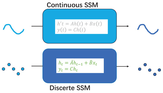
Figure 2.
Discretization of the state space model.
3.3. Skip Connection
To illustrate, consider the scenario where we have an input X, which represents the input to the system. Let us assume that we have this X, which is sent to a black box, which we will refer to as the state-space model. This model will continuously loop through the state computation and will produce the output Y. However, we can see that the of t essentially means that we The input is accepted and then jumped through the state-space model, where it is multiplied by a number D. This number is then sent directly to the output, negating the need to model D in order to model the state space. This is because D does not depend on the state system of the state space at any time step. Consequently, it can be represented as a skip connection [26]. Figure 3 provides a straightforward graphical illustration of the aforementioned text, which delineates the skip connections. Figure 4 presents a comprehensive account of the skip connections within the context of the state space model.
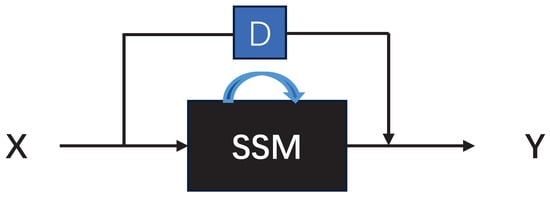
Figure 3.
Skip connections.
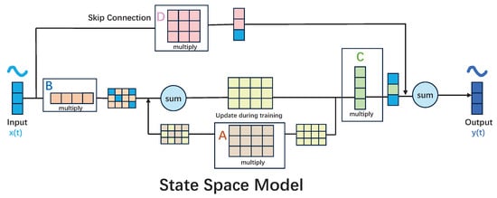
Figure 4.
The detailed process of Skip connections for the state space model.
4. Methodology
The structure of C-T-Mamba is depicted in Figure 5, composed of four primary layers. Beginning with the initial layer, a linear labeling layer encodes and labels time series inputs, embedding them into a specified space. The second layer features a single Mamba block designed to capture intricate temporal dependencies within the variables. Following this, the third layer incorporates a channel attention mechanism to compress temporal features, emphasizing critical aspects. The fourth layer integrates a temporal convolutional block comprising depth-separable convolutions and an MLP layer. Here, the depth-separable convolution captures global receptive fields and local positional characteristics, while the MLP models future time series via a linear detector head. Ultimately, a projection layer maps these temporal features to generate predictions. Detailed descriptions of each component will be elaborated in the subsequent section.
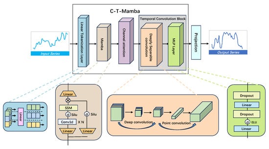
Figure 5.
General Architecture Diagram of the C-T-Mamba Model.
4.1. Linear Tokenization Layer
In processing the time-series data, we employed a methodology analogous to that utilized by iTransformer. The initial step is to tag the sequence data in order to guarantee the precision and standardization of the data. This step is of great consequence, as it directly affects the quality of the final output of the model. To achieve this goal, we employ a simple yet effective linear transformation layer. Here, the linear layer is used as a transformation tool to convert the raw time series data into a normalized form. This has the advantage of unifying the dimensions of the data, thus making it easier to compare and analyze data between different points in time.
In this context, U represents the output of the layer, represents the Batch Normalization (BatchNorm).
4.2. Mamba
4.2.1. Selective Processing of Information
In Equations (5) and (6), the parameters A, B, C, and D are identical for each input, and thus cannot be altered for each specific input. All different state-space model laws target reasoning for different inputs. Mamba’s solution is to account for a simple selection mechanism that allows the model to selectively process information in order to focus on or ignore particular inputs [21].
In particular, the authors of Mamba allow the B matrix, the C matrix, and to be functions of the inputs, thereby enabling the model to adaptively adjust its behavior in accordance with the content of the inputs. The dimensions of the B matrix, which affects the inputs, and the C matrix, which affects the state, are modified from to . This transformation corresponds to the batch size, sequence length, and hidden state size, respectively. Furthermore, the size of has been modified from D to , indicating that a distinct is associated with each token in a batch (totaling ). Notably, the B matrix, C matrix, and of each position are not identical, resulting in a unique B and C matrices for each input token. This approach effectively addresses the challenge of content awareness.
4.2.2. Parallel Scan
As mentioned earlier, since the matrices A B C are now dynamic, it is not possible to compute them using a convolutional representation (CNNs require a fixed kernel), so we have to use a cyclic representation, thus losing the parallel training capability provided by the convolution. To achieve parallelization, we investigate methodologies for computing outputs using a loop [27].
Each state, say times , plus the sum of the current input times , is called a scanning operation, and can be easily computed using a for loop, however, parallelization is not possible in this state (since each current state can only be computed if the previous state has been acquired).
The beneficial aspect of Mamba is that it facilitates eventual parallelization through the parallel scanning algorithm. This algorithm postulates that the sequence in which operations are performed is independent of the associated mathematics. Consequently, computations can be segmented and iteratively combined, as exemplified by the dynamic matrix B and the parallel scanning algorithm (see Figure 6), which collectively form the selective scanning algorithm. In the context of parallel computing, the variable t in the time complexity equation typically represents the number of processors or computing units employed to complete the task.
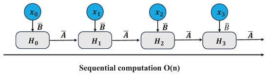
Figure 6.
Visualrepresentation of scanning operationl.
4.3. Channel Attention
While the Mamba block excels at temporal scanning, it often overlooks cross-variable dependencies in multivariate series. The Channel Attention module is strategically placed before the Mamba block to perform ‘feature screening,’ prioritizing informative variables and suppressing noise, which provides a more coherent input for global temporal modeling.
The channel attention [28,29] mechanism enhances the model’s performance by prioritizing the crucial channels within the features when processing time series data. Global pooling and average pooling operations effectively compress the features in the time dimension, distilling the information present across the entire time series. The two-layer convolutional network is capable of modeling the relationship between channels and capturing the interdependence between different channels. The outcomes of the average pooling and maximum pooling operations are aggregated after traversing the convolutional layers, respectively, to derive the integrated attention weights, as illustrated in the structural diagram in Figure 7. Ultimately, the weights are subjected to an element-level multiplication operation with the original input to obtain the weighted output [30]. This step effectively weights the features at each time step, thus emphasizing the crucial channel features.
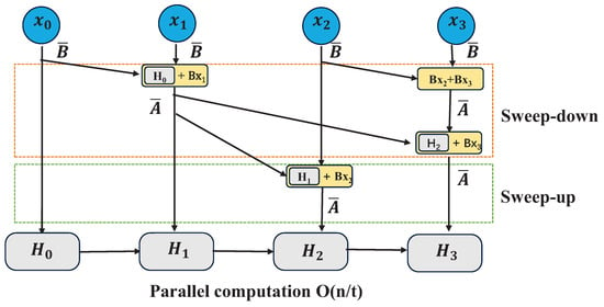
Figure 7.
Visualization of Parallel Scan.
4.4. Temporal Convolution Block
In the field of time series forecasting, most deep learning models rely on attention mechanisms to model global relationships. In contrast, our C-T-Mamba introduces a Temporal Convolutional Block, utilizing depthwise separable convolution [31] as its core module to extract local features while maintaining computational efficiency. Unlike standard convolutions, depthwise separable convolution decomposes the operation into depthwise and pointwise convolutions [32], significantly reducing parameter count and computational overhead (Figure 8). This efficiency is particularly advantageous for processing large-scale, long-term time series data in real-time scenarios. Furthermore, the integration of Multi-Layer Perceptrons (MLPs) [33] allows the model to capture complex nonlinear patterns. While convolutional layers focus on localized trends and periodicity, the fully connected structure of the MLP facilitates the learning of global features and the capture of inherent long-range dependencies.
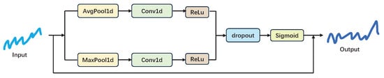
Figure 8.
Structural diagram of channel attention.
The choice of Depthwise Separable Convolution (DWConv) within the TCB is motivated by its ability to disentangle spatial (channel) and temporal correlations. Unlike standard TCNs, DWConv significantly reduces the parameter count while maintaining the receptive field size, preventing overfitting in complex multivariate scenarios. This architectural choice ensures that the local pattern extraction does not compromise the linear complexity of the overall Mamba-based framework.
4.5. Design Rationale
The synergistic integration of Channel Attention, TCB, and the Mamba block provides a transparent hierarchical feature extraction pipeline. First, the Channel Attention module acts as a “feature screener”, prioritizing informative variables while suppressing cross-channel noise. Subsequently, the TCB—utilizing multi-scale depthwise separable convolutions—extracts granular local temporal semantics that are often overlooked by pure State Space Models. Finally, the Mamba block performs long-range dependency modeling on these refined features.
Crucially, this non-parametric collaborative design significantly mitigates the risk of model misspecification. As motivated by the Hassani theorem in Section 1, traditional parametric approaches are often vulnerable to rigid distributional assumptions [18]. By combining dynamic scanning with local convolutional refinement, C-T-Mamba avoids such restrictive assumptions, ensuring robust modeling of complex, non-stationary temporal dynamics while maintaining linear computational efficiency.
5. Experiments
5.1. Multivariate Long-Term Forecasting
Datset: The datasets are as follows: The present study employs five widely utilized multivariate time series datasets for the purpose of forecasting. The detailed statistics of the dataset sizes are provided in the following section. (1) ETTm(1,2) contains time series of non-stationary factors related to oil volume and electrical loads, as observed in electric transformers from July 2016 to July 2018. (2) Traffic is a collection of 48 months (2015–2016) of hourly data from the California Department of Transportation. The data set describes the occupancy of roadways (measured on a scale of 0 to 1) as observed by sensors deployed on freeways in the San Francisco Bay Area. (3) Exchange. The Exchange dataset compiles daily exchange rates for eight countries from 1990 to 2016. (4) The ECL dataset contains the hourly electricity consumption of 321 customers from 2012 to 2014.
We selected these five datasets (ETT, Traffic, Exchange, and ECL) because they represent diverse real-world scenarios with distinct temporal characteristics: ETT reflects highly periodic electrical load patterns; Traffic and ECL capture human activity dynamics; while Exchange represents financial fluctuations with relatively weak seasonality. This diversity enables a comprehensive evaluation of the model’s generalization capability across both stationary and non-stationary time series. Table 1 describes in detail the number of variables, sampling frequency, and total observations for these data sets.

Table 1.
Statistical information on the five data sets.
All datasets are split into training, validation, and test sets with a ratio of 7:2:1. To prevent data leakage, we utilized a chronological split without shuffling, ensuring the model is always tested on “future” data relative to the training set.
Baselines: A comparative analysis of the models was conducted, in which our model was evaluated in conjunction with five representative and state-of-the-art (SOTA) predictive models. These included:Transformer-based methods, namely iTransformer, PatchTST, and Autoformer;Linear-based methods, specifically TiDE; and Time-convolutional network-based methods. A concise overview of these models is provided below.
- The iTransformer [34] reverses the responsibilities of the attention mechanism and the feedforward network. Specifically, the time points of individual series are embedded in variable tokens, which are utilized by the attention mechanism to capture multivariate correlations. Concurrently, a feedforward network is applied to each variable token to learn the nonlinear representation.
- PatchTST [35] presents an efficient design of a transformer-based time series prediction task model, introducing two key components: patch and channel-independent structures. It captures local semantic information and benefits from a longer backtracking window than previous work. The model has been shown to outperform other baselines in supervised learning, and also demonstrates its power in self-supervised representation learning and migration learning.
- The Autoformer [10] is a decomposition architecture that progressively aggregates the long-term trend component from intermediate forecasts by embedding series decomposition blocks as internal operators. Furthermore, an efficient autocorrelation mechanism is designed to perform dependency discovery and information aggregation at the series level, which contrasts with the previous auto-attention family. The autoformer naturally achieves complexity and produces consistent state-of-the-art performance across a wide range of realistic datasets.
- TiDE [16] presents a simple MLP-based encoder-decoder model that exhibits performance comparable to or superior to existing neural network baselines on widely utilized long-term prediction benchmarks. Concurrently, TiDE operates at a processing speed that is 5–10 times faster than the most efficient Transformer-based baselines. The study posits that, at least with respect to these long-term prediction benchmarks, the identification of periodicity and trend patterns may not necessitate self-referential processes.
- The TimesNet [15] model serves as a foundational framework for time series analysis, driven by multi-periodicity. Its modular architecture enables the elucidation of complex temporal variations, while parameter-efficient starting blocks facilitate the capture of intra-periodic and inter-periodic variations in two-dimensional space. The versatility and performance of TimesNet have been demonstrated in five mainstream analysis tasks through experimental investigation.
Parameter setting: The following section outlines the parameter settings utilized in the experiment. All experiments were conducted on a NVIDIA RTX 3090 (24 GB) (NVIDIA, Santa Clara, CA, USA), with a single Mamba block and a single temporal convolution block. The initial learning rate was adjusted to . The early stopping strategy was set to three, the batch size was set to either 16 or 32, the number of train epochs was set to 10, and the number of neurons in the fully connected layer of the model was adjusted to 128, 256, or 512.
Metric: We use two evaluation metrics, including
5.2. Overall Performance
Table 2 depicts the experimental outcomes of the six models on five datasets. The optimal results for MSE are indicated in black bold, while the optimal results for MAE are indicated in red bold. As evidenced by the data in the table, the last row of our model exhibits the The highest number of wins indicates that the generalization ability of our model is superior to that of the other five models. Our model outperforms the best PatchTST based on the Transformer architecture and PatchTST, as well as TimesNet based on CNN architecture. This demonstrates that our model’s performance is superior.
Table 2.
Multivariate forecasting results with prediction lengths . We fix the lookback length T = 96. All the results are averaged from all prediction lengths. The smaller the MSE, MAE, the more accurate the prediction results. Detailed results with standard deviations are provided in Appendix A.2.
The MSE and MAE of iTransformer on ETTm1 and ETTm2 on these two datasets demonstrate superior performance within certain prediction windows (e.g., 192 and 336), yet in general, they are not as effective. These results are comparable to those of C-T-Mamba and PatchTST, which may be attributed to the use of linear layers for data embedding in iTransformer. While this approach is relatively straightforward, it may not be sufficient for capturing the temporal features present in complex datasets. Indeed, the ETT dataset is more complex than the other three datasets, as it combines short-term cyclical patterns, long-term cyclical patterns, long-term trends, and numerous irregular patterns. This aligns with the findings of our analysis. iTransformer The full-attention mechanism of iTransformer is capable of capturing long- and short-term dependencies. However, its computational complexity is considerable, and it may encounter performance bottlenecks when dealing with large-scale data.
The proposed model demonstrates inferior performance compared to PatchTST in the two datasets, ETTm1 and ETTm2. In fact, the proposed model exhibits only marginally superior performance, likely due to the reduced number of variables, the intricate temporal features, and the fusion of multiple temporal features in the dataset. Additionally, the channel attention mechanism is unable to effectively extract temporal dependencies from the complex features, or the extracted temporal dependencies are insufficient, resulting in the observed ineffectiveness.
Furthermore, to assess the predictive capacity of C-T-Mamba in a more intuitive manner, we present a visual comparison of the prediction outcomes of C-T-Mamba and the remaining five benchmarks on our ECL dataset, as illustrated in Figure 9. Specifically, a variable was randomly selected and its backward sequence was input. The true sequence is represented by the blue line, and the model’s prediction is represented by the red line in the following Figure 9. It is evident that the prediction results of C-T-Mamba are in close proximity to the actual values and superior to the other five baseline models on the ECL dataset.
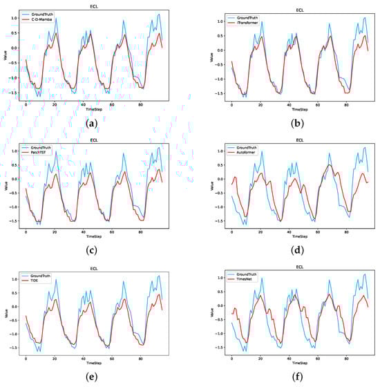
Figure 9.
Visualization of 96 outcomes on ECL dataset predicted by All models. (a) C-T-Mamba; (b) iTranformer; (c) PatchTST; (d) Autoformer; (e) TiDE; (f) TimesNet.
5.3. Ablation Experiment
To assess the effectiveness of the constituent elements of C-T-Mamba, we conducted an ablation study, whereby channel attention and temporal convolution block were removed. C-Mamba comprises solely a Mamba block and a channel attention component, while T-Mamba incorporates only a Mamba block and a temporal convolution block component. In contrast, Mamba is devoid of both channel attention and temporal convolution block, relying solely on a unidirectional Mamba block.The detailed ablation experimental results on the ETTm1, ETTm2, and ECL datasets are shown in Table 3.
Table 3.
Complete results of ETTm1, ETTm2, and ECL ablation studies. We fixed the backtracking window and made predictions for . Bolded fonts with colors indicate the best results.
5.3.1. Look-Back Window
To investigate whether model performance scales consistently with the expansion of the look-back window, we conducted experiments on the Traffic and ECL datasets. By fixing the label and prediction lengths while incrementally increasing the input sequence length (), we tested the hypothesis that a broader receptive field enhances the capture of long-range temporal dependencies.The experimental results, illustrated in the accompanying Figure 10, reveal a counterintuitive trend: the predictive accuracy of the Informer, Reformer, and Transformer models fails to improve—and in some cases degrades—as the retrospective window extends. This phenomenon may be attributed to the inherent limitations of the self-attention mechanism; specifically, as the sequence length increases, the attention maps often become increasingly sparse or “diluted”. This causes the model to over-index on local fluctuations while losing the ability to extract coherent global patterns.In contrast, our proposed model maintains superior performance across varying window lengths (see Figure 10). By integrating depthwise separable convolutions with Multilayer Perceptrons (MLPs) within the convolutional block, our architecture effectively balances the extraction of fine-grained local features with the integration of global temporal contexts. This structural synergy appears to be a primary factor in overcoming the sequence-length bottleneck observed in pure attention-based architectures.
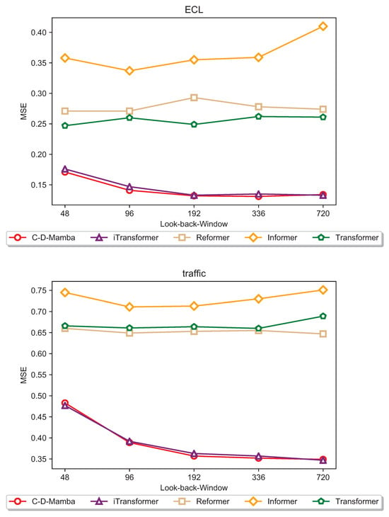
Figure 10.
Prediction performance for both Traffic and ECL datasets with backtracking length L 96, 192, 336, 720 and prediction length T = 96 for both datasets.
5.3.2. Operational Efficiency Analysis
A comprehensive comparison of GPU memory utilization and inference runtime across temporal feature extraction components provides clear quantitative evidence of our model’s computational advantages. As illustrated in Figure 11, both the MambaBlock and its auxiliary modules—Channel Attention and the Temporal Convolution Block—demonstrate near-linear scaling behavior with respect to sequence length. This trend contrasts sharply with the AutoCorrelation and FullAttention mechanisms, whose resource demands increase superlinearly.
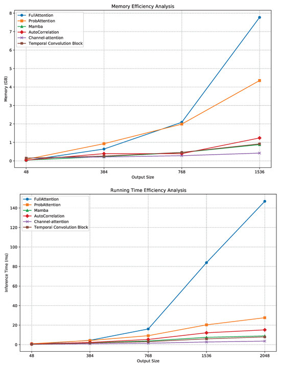
Figure 11.
Efficiency analysis of various components for extracting temporal features.
Empirically, GPU memory usage for MambaBlock grows modestly from 0.04 GB at L = 48 to 0.88 GB at L = 1536, whereas AutoCorrelation rises to 1.24 GB under the same conditions, implying an approximate 29% reduction in peak memory cost. Similarly, inference latency increases linearly from 0.52 ms to 8.9 ms for MambaBlock, compared to 12.1 ms for AutoCorrelation, confirming a lower empirical complexity than the theoretical bound associated with correlation-based attention.
Figure 11 further indicates that Channel Attention achieves the best memory–latency trade-off, reflecting its lightweight gating mechanism that amplifies channel selectivity with minimal overhead. In contrast, the FullAttention and ProbAttention variants exhibit substantially higher runtime slopes, consistent with quadratic dependency on sequence length.
These findings jointly demonstrate that our proposed C–T–Mamba architecture achieves superior operational efficiency, balancing long-range temporal dependency modeling with reduced computational cost. The empirical runtime slope closely approximates linear growth, validating the theoretical design goal of sub– complexity. Consequently, C–T–Mamba presents a scalable and resource-efficient framework for high-dimensional time series forecasting tasks.
6. Conclusions
In this paper, we introduce C-T-Mamba, a novel long-term time series forecasting model built upon the Mamba framework. C-T-Mamba leverages a hybrid architecture incorporating channel mixing and temporal convolutional blocks. This innovative design enables the model to discern extended temporal trends while mitigating redundancy, thereby effectively extracting pivotal local and global insights to enhance forecasting accuracy. Validation of our experimental findings across five publicly available datasets underscores the model’s robust forecasting performance and computational efficiency, rendering it a promising solution across diverse forecasting domains. The exploration of channel independence and mixing in temporal series represents a burgeoning area of interest among researchers. Our utilization of channel mixing for temporal feature extraction in this study sets a foundation for future investigations into the efficacy of channel independence in time series forecasting, alongside further exploration of the Mamba model’s potential in this domain.
Discussions and Limitations
Although C-T-Mamba achieves superior efficiency and accuracy, it has limitations. First, while TCB captures local semantics, the optimal kernel size may vary across different data frequencies. Second, our study primarily focuses on five public benchmarks; its robustness in extremely noisy or irregular sampling scenarios (e.g., medical streaming data) requires further validation. In future work, we aim to explore adaptive kernel mechanisms and extend the framework to real-time online forecasting tasks.
Author Contributions
W.G.: Project management, Supervision, Writing—review. R.L.: Writing original draft. S.Y.: Software programming. All authors have read and agreed to the published version of the manuscript.
Funding
This work was supported by the Open Fund of the Key Laboratory of Geological Hazards on the Three Gorges Reservoir (China Three Gorges University) (Grant No. 2022KDZ05), and the National Natural Science Foundation of China (Grant No. 62171327), entitled “Theory and Methods of Visible and Infrared Image Fusion Taking into Account Semantic Information and Cross-Modal Representation”.
Data Availability Statement
The datasets used and analysed during the current study available from the corresponding author on reasonable request.
Conflicts of Interest
The authors declare that they have no known competing financial interests or personal relationships that could have appeared to influence the work reported in this paper.
Appendix A. Implementation Details
Appendix A.1. Hyperparameters
Data Preprocessing and Splitting. To ensure a rigorous and fair evaluation, all datasets used in our experiments were processed following the standard protocol in long-term time series forecasting (LTSF). Specifically:
Random Seeds: To ensure the reliability and reproducibility of our results, all experiments were conducted using 5 independent runs with different random seeds: .The final performance metrics (MSE and MAE) are reported as the average values across these runs.
Data Splitting: For the ETT datasets (ETTm1, ETTm2), we followed the official split (12:4:4 months for training, validation, and testing). For other custom datasets (Electricity, Traffic, Weather), we adopted a chronological split ratio of 7:2:1, as implemented in our class.
Normalization: We applied Z-score standardization to each variable independently. The mean and standard deviation were computed solely from the training set to prevent any data leakage from the validation or testing phases.
Model Architecture and Hyperparameters. C-T-Mamba was implemented using PyTorch 2.0. The core architecture comprises a Mamba backbone, a Channel Attention module, and a Temporal Convolutional Block (TCB). The hyperparameter configurations are detailed below:
Sequence Lengths: For all experiments, the lookback window size L was fixed at 96, while the prediction horizons T were set to . Module Specifics:
Mamba Block: The state dimension was dynamically adjusted based on dataset complexity. As shown in our training scripts, we utilized for smaller datasets (ETT, Weather) to prevent overfitting, and for high-dimensional datasets (Electricity, Traffic) to capture intricate cross-dimension dependencies.
TCB: The Temporal Convolutional Block utilized depthwise separable convolutions with a fixed kernel size of 3, stride of 1, and ELU activation.
Optimization Strategy: We used the Adam optimizer with a batch size of 16 or 32. The learning rate was tuned via grid search within the range . Specifically: For ETTm1/m2, a lower learning rate of was used.For Traffic/Electricity, the learning rate was set between and to accommodate the larger feature space.
Training Details: All models were trained for 5 to 10 epochs (e.g., 5 epochs for Electricity and Traffic) with an early stopping mechanism (patience of 3) to ensure convergence.
Hardware and Software Environment. All experiments were conducted on a workstation equipped with NVIDIA RTX 3090 (24GB VRAM) GPUs. The software environment included Ubuntu 20.04, Python 3.8, and CUDA 11.8. To ensure the reliability of our results, all metrics reported (MSE and MAE) are averaged over 5 independent runs with different random seeds, as detailed in the statistical analysis in Appendix A.2.
Appendix A.2. Statistical Stability Analysis
Table A1.
Detailed Forecasting Results (Mean ± Std) for C-T-Mamba.
Table A1.
Detailed Forecasting Results (Mean ± Std) for C-T-Mamba.
| Dataset | ETTm1 | ETTm2 | Traffic | Exchange | ECL | |
|---|---|---|---|---|---|---|
| Horizon | ||||||
| 96 | MSE | |||||
| MAE | ||||||
| 192 | MSE | |||||
| MAE | ||||||
| 336 | MSE | |||||
| MAE | ||||||
| 720 | MSE | |||||
| MAE | ||||||
References
- Lim, B.; Zohren, S. Time-series forecasting with deep learning: A survey. Philos. Trans. R. Soc. A 2021, 379, 20200209. [Google Scholar] [CrossRef] [PubMed]
- Torres, J.F.; Hadjout, D.; Sebaa, A.; Martínez-Álvarez, F.; Troncoso, A. Deep learning for time series forecasting: A survey. Big Data 2021, 9, 3–21. [Google Scholar] [CrossRef] [PubMed]
- Tang, H.; Zhang, C.; Jin, M.; Yu, Q.; Wang, Z.; Jin, X.; Du, M. Time series forecasting with LLMs: Understanding and enhancing model capabilities. ACM SIGKDD Explor. Newsl. 2025, 26, 109–118. [Google Scholar] [CrossRef]
- Blázquez-García, A.; Conde, A.; Mori, U.; Lozano, J.A. A review on outlier/anomaly detection in time series data. Acm Comput. Surv. (CSUR) 2021, 54, 1–33. [Google Scholar] [CrossRef]
- Gillioz, A.; Casas, J.; Mugellini, E.; Abou Khaled, O. Overview of the Transformer-based Models for NLP Tasks. In Proceedings of the 2020 15th Conference on Computer Science and Information Systems (FedCSIS), Sofia, Bulgaria, 6–9 September 2020; pp. 179–183. [Google Scholar]
- Kim, J.; Kim, H.; Kim, H.; Lee, D.; Yoon, S. A comprehensive survey of deep learning for time series forecasting: Architectural diversity and open challenges. Artif. Intell. Rev. 2025, 58, 1–95. [Google Scholar] [CrossRef]
- Sherstinsky, A. Fundamentals of recurrent neural network (RNN) and long short-term memory (LSTM) network. Phys. D Nonlinear Phenom. 2020, 404, 132306. [Google Scholar] [CrossRef]
- Abbasimehr, H.; Paki, R. Improving time series forecasting using LSTM and attention models. J. Ambient. Intell. Humaniz. Comput. 2022, 13, 673–691. [Google Scholar] [CrossRef]
- Zhou, H.; Zhang, S.; Peng, J.; Zhang, S.; Li, J.; Xiong, H.; Zhang, W. Informer: Beyond efficient transformer for long sequence time-series forecasting. In Proceedings of the AAAI Conference on Artificial Intelligence, Vancouver, Canada, 2–9 February 2021; Volume 35, pp. 11106–11115. [Google Scholar]
- Wu, H.; Xu, J.; Wang, J.; Long, M. Autoformer: Decomposition transformers with auto-correlation for long-term series forecasting. Adv. Neural Inf. Process. Syst. 2021, 34, 22419–22430. [Google Scholar]
- Kitaev, N.; Kaiser, L.; Levskaya, A. Reformer: The Efficient Transformer. In Proceedings of the International Conference on Learning Representations (ICLR), Addis Ababa, Ethiopia, 26–30 April 2020. [Google Scholar]
- Zhou, T.; Ma, Z.; Wen, Q.; Wang, X.; Sun, L.; Jin, R. Fedformer: Frequency enhanced decomposed transformer for long-term series forecasting. In Proceedings of the International Conference on Machine Learning PMLR, Baltimore, MD, USA, 17–23 July 2022; pp. 27268–27286. [Google Scholar]
- Zhang, Y.; Yan, J. Crossformer: Transformer utilizing cross-dimension dependency for multivariate time series forecasting. In Proceedings of the The Eleventh International Conference on Learning Representations, Kigali, Rwanda, 1–5 May 2023. [Google Scholar]
- Yi, K.; Zhang, Q.; Fan, W.; He, H.; Hu, L.; Wang, P.; An, N.; Cao, L.; Niu, Z. FourierGNN: Rethinking multivariate time series forecasting from a pure graph perspective. Adv. Neural Inf. Process. Syst. 2024, 36, 69638–69660. [Google Scholar]
- Wu, H.; Hu, T.; Liu, Y.; Zhou, H.; Wang, J.; Long, M. TimesNet: Temporal 2D-Variation Modeling for General Time Series Analysis. In Proceedings of the Eleventh International Conference on Learning Representations (ICLR), Kigali, Rwanda, 1–5 May 2023. [Google Scholar]
- Das, A.; Kong, W.; Leach, A.; Mathur, S.; Sen, R.; Yu, R. Long-term Forecasting with TiDE: Time-Series Dense Encoder. arXiv 2023, arXiv:2304.08424. [Google Scholar]
- Dao, T.; Gu, A. Transformers are SSMs: Generalized Models and Efficient Algorithms Through Structured State Space Duality. Proc. Mach. Learn. Res. 2024, 235, 10041–10071. [Google Scholar]
- Hassani, H. Singular spectrum analysis: Methodology and comparison. J. Data Sci. 2007, 5, 239–257. [Google Scholar] [CrossRef]
- Lieber, O.; Lenz, B.; Bata, H.; Cohen, G.; Osin, J.; Dalmedigos, I.; Safahi, E.; Meirom, S.; Belinkov, Y.; Shalev-Shwartz, S.; et al. Jamba: A hybrid transformer-mamba language model. arXiv 2024, arXiv:2403.19887. [Google Scholar] [CrossRef]
- Ma, X.; Zhang, X.; Pun, M.O. RS 3 Mamba: Visual State Space Model for Remote Sensing Image Semantic Segmentation. IEEE Geosci. Remote Sens. Lett. 2024, 21, 6011405. [Google Scholar] [CrossRef]
- Cai, X.; Zhu, Y.; Wang, X.; Yao, Y. MambaTS: A Mamba-based Backbone for Time Series Forecasting. arXiv 2024, arXiv:2405.00403. [Google Scholar]
- Wang, Z.; Kong, F.; Feng, S.; Wang, M.; Yang, X.; Zhao, H.; Zhang, Y. Is mamba effective for time series forecasting? Neurocomputing 2025, 619, 129178. [Google Scholar] [CrossRef]
- Ahamed, M.A.; Cheng, Q. TimeMachine: A Dual-path Mamba Network for Long-term Time Series Forecasting. arXiv 2024, arXiv:2403.09898. [Google Scholar]
- Zhou, W.; Kamata, S.I.; Wang, H.; Wong, M.S.; Hou, H.C. Mamba-in-Mamba: Centralized Mamba-Cross-Scan in Tokenized Mamba Model for Hyperspectral Image Classification. Neurocomputing 2025, 613, 128751. [Google Scholar] [CrossRef]
- Ma, J.; Li, F.; Wang, B. U-mamba: Enhancing long-range dependency for biomedical image segmentation. arXiv 2024, arXiv:2401.04722. [Google Scholar]
- Terwilliger, P.; Sarle, J.; Walker, S.; Harrivel, A. A ResNet Autoencoder Approach for Time Series Classification of Cognitive State. In Proceedings of the MODSIM World, Norfolk, VA, USA, 5–7 May 2020; pp. 1–11. [Google Scholar]
- Xin, X.; Deng, Y.; Huang, W.; Wu, Y.; Fang, J.; Wang, J. Multi-Pattern Scanning Mamba for Cloud Removal. Remote Sens. 2025, 17, 3593. [Google Scholar] [CrossRef]
- Wang, Q.; Wu, B.; Zhu, P.; Li, P.; Zuo, W.; Hu, Q. ECA-Net: Efficient channel attention for deep convolutional neural networks. In Proceedings of the IEEE/CVF Conference on Computer Vision and Pattern Recognition, Seattle, WA, USA, 13–19 June 2020; pp. 11534–11542. [Google Scholar]
- Choi, M.; Kim, H.; Han, B.; Xu, N.; Lee, K.M. Channel attention is all you need for video frame interpolation. In Proceedings of the AAAI Conference on Artificial Intelligence, New York, NY, USA, 7–12 February 2020; Volume 34, pp. 10663–10671. [Google Scholar]
- Bhuyan, P.; Singh, P.K.; Das, S.K. Res4net-CBAM: A deep cnn with convolution block attention module for tea leaf disease diagnosis. Multimed. Tools Appl. 2024, 83, 48925–48947. [Google Scholar] [CrossRef]
- Chen, J.; Lu, Z.; Xue, J.H.; Liao, Q. XSepConv: Extremely Separated Convolution. IEEE Trans. Image Process. 2020, 29, 5639–5653. [Google Scholar]
- Liu, M.; Xia, C.; Xia, Y.; Deng, S.; Wang, Y. TDCN: A Novel Temporal Depthwise Convolutional Network for Short-Term Load Forecasting. Int. J. Electr. Power Energy Syst. 2025, 165, 110512. [Google Scholar] [CrossRef]
- Yu, T.; Li, X.; Cai, Y.; Sun, M.; Li, P. S2-mlp: Spatial-shift mlp architecture for vision. In Proceedings of the IEEE/CVF Winter Conference on Applications of Computer Vision, Waikoloa, HI, USA, 3–8 January 2022; pp. 297–306. [Google Scholar]
- Liu, Y.; Hu, T.; Zhang, H.; Wu, H.; Wang, S.; Ma, L.; Long, M. iTransformer: Inverted Transformers Are Effective for Time Series Forecasting. In Proceedings of the Twelfth International Conference on Learning Representations (ICLR), Vienna, Austria, 7–11 May 2024. [Google Scholar]
- Nie, Y.; Nguyen, N.H.; Sinthong, P.; Kalagnanam, J. A Time Series is Worth 64 Words: Long-term Forecasting with Transformers. In Proceedings of the International Conference on Learning Representations (ICLR), Kigali, Rwanda, 1–5 May 2023. [Google Scholar]


Disclaimer/Publisher’s Note: The statements, opinions and data contained in all publications are solely those of the individual author(s) and contributor(s) and not of MDPI and/or the editor(s). MDPI and/or the editor(s) disclaim responsibility for any injury to people or property resulting from any ideas, methods, instructions or products referred to in the content. |
© 2026 by the authors. Licensee MDPI, Basel, Switzerland. This article is an open access article distributed under the terms and conditions of the Creative Commons Attribution (CC BY) license.