RTDNet: Modulation-Conditioned Attention Network for Robust Denoising of LPI Radar Signals

Abstract

Accurate processing of low-probability-of-intercept (LPI) radar signals poses a critical challenge in electronic warfare support (ES). These signals are often transmitted at very low signal-to-noise ratios (SNRs), making reliable analysis difficult. Noise interference can lead to misinterpretation, potentially resulting in strategic errors and jeopardizing the safety of friendly forces. Accordingly, effective noise suppression techniques that preserve the original waveform shape are crucial for reliable analysis and accurate parameter estimation. In this study, we propose the recognize-then-denoise network (RTDNet), which effectively removes noise while minimizing signal distortion. The proposed approach first employs a modulation recognition network to infer the modulation scheme and then feeds the inferred label to an attention-based denoiser to guide feature extraction. By leveraging prior information, the attention mechanism preserves key features and reconstructs challenging patterns such as polytime and polyphase codes. Simulation results indicate that RTDNet more effectively removes noise while maintaining the waveform shape and salient signal structures compared with existing techniques. Furthermore, RTDNet improves modulation classification accuracy and parameter estimation performance. Finally, its compact model size and fast inference meet the performance and efficiency requirements of ES missions.

1. Introduction

Electronic warfare support (ES) activities involve collecting, processing, and analyzing information to identify adversaries’ locations, movements, and intentions. These activities are essential for planning friendly defensive and offensive electronic warfare (EW) operations [1,2]. However, in practical ES pipelines, signals are often severely corrupted by low signal-to-noise ratio (SNR), which drastically degrades the performance of subsequent analyses such as modulation recognition and parameter estimation. In particular, low-probability-of-intercept (LPI) radar, widely used in EW, evades detection by transmitting at low power. Consequently, its signals suffer significant attenuation over long distances and under high-frequency carrier conditions, causing the received SNR to often fall below 0 dB [3]. Furthermore, LPI radar employs diverse nonstationary modulation schemes, making analysis even more difficult [3,4]. Therefore, effective denoising of LPI radar signals is a prerequisite for ensuring the reliability and robustness of the ES pipeline. More broadly, signal restoration under non-ideal conditions has been actively studied across radar modalities. For example, recent studies on deceptive jammer localization and suppression in multichannel SAR (synthetic aperture radar) [5] and multistatic SAR [6] emphasize the practical importance of recovering reliable signal structures in the region of interest by suppressing deception-induced artifacts such as false targets. From this perspective, robust denoising is a critical prerequisite for reliable radar signal analysis, and this paper focuses on denoising low-SNR LPI radar signals in ES pipelines.

1.1. Related Work

Both traditional and deep learning-based approaches have been extensively studied for denoising LPI radar signals. Among traditional methods, wavelet-based techniques such as the Gaussian wavelet [7] and modified sinc wavelet [8], as well as mode decomposition strategies like ensemble empirical mode decomposition (EEMD) [9] and hybrid variational mode decomposition [10], are representative examples. Although the Gaussian wavelet is advantageous for extracting low-frequency components, it has the limitation of a non-flat frequency response. The modified sinc wavelet, which has a flatter response, aims to enhance noise rejection performance over a wide band. Mode decomposition-based approaches have also been reported to separate and refine the signal components and noise, simultaneously improving waveform preservation and recognition performance at low SNR. Nevertheless, when applied to low-SNR LPI signals, these traditional methods are vulnerable to signal nonstationarity, often leading to signal distortion or residual noise that degrades the performance of subsequent tasks such as modulation recognition [11].

Deep learning approaches have further improved denoising performance by learning the complex characteristics of signals. Models such as DnCNN (denoising convolutional neural network) [12], which uses residual learning and batch normalization; U2Net [13,14], a modified U-Net structure derived from semantic segmentation; and GAN (generative adversarial network)-based models [15,16] that utilize adversarial learning between a generator and discriminator have been reported. In addition, self-supervised denoising frameworks have been explored to reduce the need for clean training targets. For example, blind-spot masking schemes such as Noise2Void [17] and Noise2Self [18] learn denoisers from only noisy observations by masking parts of the input and predicting them during training. These approaches, however, rely on strong assumptions such as conditional noise independence and unbiased noise, which are often difficult to guarantee in practical ES conditions. They may also become less reliable when the SNR is extremely low, and the signal evidence is weak. As a result, waveform distortion-where the signal’s intrinsic structure is damaged during denoising-can still occur, limiting the accuracy of subsequent stages.

In parallel, recent research on LPI radar modulation recognition has advanced in both learning strategies and architectures. In terms of learning strategies, supervised learning remains predominant, while semi-supervised schemes such as mean teacher [19] and low-SNR-adaptive temporal masking [20] have been reported to improve generalization under limited-label and low-SNR conditions. Additionally, unsupervised recognition has been explored for unlabeled radar signals by combining time–frequency representations with subspace-clustering techniques [21]. Self-supervised representation learning has also been studied to reduce the reliance on labeled data by pretraining on abundant unlabeled TFIs and then fine-tuning for modulation classification using only a small labeled set [22], but such approaches remain less mature than supervised models for precise LPI modulation recognition at very low SNRs. On the architectural front, various efficient designs have been proposed, including X-net-style CNN backbones [23] and cross-scale CNNs for multi-resolution feature extraction [24]. Furthermore, Transformer variants, CNN-Vision-Transformer hybrids [25,26], and EfficientNet-based designs [27] have been introduced to further enhance recognition performance. The combination of these advances has shown significant improvements in modulation recognition performance at low SNRs, with some studies reporting the feasibility of recognizing various modulated signals even at SNRs around or below $-10$ dB [28,29].

1.2. Motivation and Contributions

As recent studies have shown that reliable modulation recognition is feasible even at low SNR, this study proposes a recognize-then-denoise network (RTDNet) that first recognizes the modulation scheme (recognize) and then leverages this information to minimize distortion during denoising (denoise). RTDNet first estimates the modulation scheme using a classifier and injects this information as a condition into an attention-driven denoising backbone to suppress noise while preserving the signal structure. The key motivation is that, in very low-SNR regimes, conventional denoisers that operate without waveform-specific priors can inadvertently remove or deform modulation-dependent time–frequency structures, which can directly degrade subsequent ES analysis tasks such as radar-parameter estimation. Meanwhile, most recognition methods assume that the input representation preserves such structures and are typically applied after denoising as a separate stage. RTDNet addresses this gap by explicitly coupling recognition and denoising, using the recognized modulation information as a prior to guide the denoiser toward modulation-consistent restoration and reduce waveform distortion in low-SNR environments.

The key contributions of this study are as follows:

1.

Incorporating modulation information as prior knowledge enabled the network to ensure distortion-free denoising tailored to each modulation type.

2.

Effective denoising was achieved by employing an attention mechanism that enhances the distinction between signal and noise. Noise removal performance was further improved by focusing on relevant signal regions.

3.

The resulting time–frequency images (TFIs) boost the accuracy of the same classifier and yield more precise parameter estimates than those obtained with existing methods across the entire SNR range.

The remainder of this paper is organized as follows: Section 2 introduces the LPI radar model and data preprocessing. Section 3 details the RTDNet architecture and attention design. Section 4 presents the simulation results and comparisons with baseline models. Finally, Section 5 concludes the paper.

2. Background

2.1. LPI Radar Signal Model

The LPI radar signal $y\left(t\right)$ received by the ES system can be expressed as the sum of the modulated signal $s\left(t\right)$ and additive white Gaussian noise (AWGN) $n\left(t\right)$, as indicated in (1).

$$y\left(t\right)=s\left(t\right)+n\left(t\right)=a\left(t\right)\exp (j2\pi f_{k}t+j{\varphi }_k)+n\left(t\right).$$

(1)

Here, $a\left(t\right)=A$ for $0\le t<{\tau }_{\mathrm{pw}}$ (that is, it remains constant within a pulse of width ${\tau }_{\mathrm{pw}}$), and each pulse repeats periodically with the pulse repetition interval. Parameters $f_k$ and ${\varphi }_k$ represent the frequency and phase values determined by the modulation scheme, respectively. In frequency modulation, $f_k$ varies while ${\varphi }_k$ remains fixed. In phase modulation, ${\varphi }_k$ varies while $f_k$ remains fixed. LPI radar utilizes both schemes to minimize interception and complicate detection by adversary systems. In this study, two frequency-modulated waveforms were considered: linear frequency modulation (LFM) and the Costas code. Ten phase-modulated waveforms were also utilized: the Barker code, polyphase codes (Frank, P1, P2, P3, and P4), and polytime codes (T1, T2, T3, and T4). Incorporating an unmodulated rectangular pulse yields a total of 13 waveform types [3].

2.2. Choi-Williams Distribution (CWD)

Radar time–frequency analysis can employ the short-time Fourier transform (STFT), Wigner-Ville distribution (WVD), or CWD [30]. In this study, we utilized CWD, which is well-suited to radar signals because it effectively suppresses cross-terms. CWD retains key signal structures while minimizing artifacts, providing higher resolution than STFT and fewer cross-terms than WVD. CWD is a member of Cohen’s time–frequency class. It employs an exponential kernel that serves as a low-pass filter in the ambiguity domain, and a two-dimensional Fourier transform yields the distribution [29]. The kernel function used in this study is defined as follows:

$$G(\xi ,\tau )=e^{-{\xi }^2{\tau }^2/\sigma },$$

(2)

where $\xi$, $\tau$, and $\sigma$ represent the Doppler frequency shift, time delay, and constant scale factor that control cross-term suppression in the time–frequency distribution, respectively. In this study, $\sigma$ was set to 1 to effectively suppress the cross-terms while maintaining the essential signal characteristics. The equation for the received signal $y\left(t\right)$ using CWD is

$$\begin{array}{c}\hfill CW{D}_y(t,\omega )={\displaystyle {\int }_{-\infty }^{+\infty }}{e}^{-j\omega \tau }{\int }_{-\infty }^{+\infty }\sqrt{{\displaystyle \frac{\sigma }{4\pi {\tau }^2}}}{e}^{-{\displaystyle \frac{\sigma {(u-t)}^2}{4{\tau }^2}}}\times y\left(u+{\displaystyle \frac{\tau }{2}}\right)y^{*}\left(u-{\displaystyle \frac{\tau }{2}}\right)dud\tau ,\end{array}$$

(3)

where t and $\omega$ represent the time and angular frequency variables, respectively, and $y^{*}$ represents the complex conjugate of the signal y.

3. Proposed Method

This section presents RTDNet, a recognize-then-denoise framework that conditions the denoiser on the estimated modulation prior. Figure 1 illustrates the overall framework of RTDNet. The received LPI radar signal is first converted into a TFI to capture temporal variations. The modulation recognition network then estimates the modulation scheme and produces a probability vector p. To reduce computational burden, a scaling stage compresses the spatial resolution of the TFI. The resized TFI and the estimated modulation information are jointly fed into the attention-driven denoising backbone, where modulation-conditioned cross-attention injects the prior into the feature maps to guide restoration. Finally, a postscaling stage restores the original resolution. This modulation-conditioned denoising is designed to preserve modulation-consistent structures while suppressing noise in low-SNR environments.

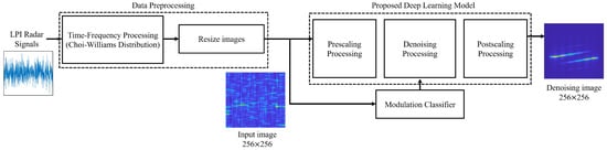
Figure 1. Overall framework of the proposed denoising method.

3.1. RTDNet Architecture

RTDNet is a modulation-conditioned denoiser: an auxiliary recognizer estimates a modulation prior, and the denoiser uses this prior to guide the denoising of LPI radar signals. The modulation recognition network classifies each input TFI into one of the 13 waveform types and outputs the corresponding probability vector p. The denoising network follows an encoder–decoder architecture that combines attention with the modulation prior. At inference, the logits are passed directly to the denoiser, embedded, and then entered into the cross-attention layers. Since modulation is recognized first, the denoiser can adapt its processing to the most likely waveform, focus on relevant features, and suppress other noise effectively.

Figure 2 shows the denoising network architecture, and Table 1 lists the layer-by-layer configuration. For each stage, the table reports the repetition count r and the output tensor size $H_{\mathrm{out}},W_{\mathrm{out}},C_{\mathrm{out}}$, which determine the computational cost of each block. The denoising backbone comprises a scaling stage followed by a denoising stage. The scaling stage employs convolutional layers for downsampling and upsampling. It compresses feature maps to reduce the computational cost while capturing the global structure and then restores a denoised TFI to its original size. The denoising stage consists of a sequence of residual convolutions and attention blocks that progressively refine the features and remove noise. Three stacked feature enhancement (FE) layers extract the local patterns before further downsampling. A single bottleneck layer captures the global context at the coarsest scale. Three symmetric feature reconstruction (FR) layers are then upsampled to full resolution with skip connections. Section 3.2 and Section 3.3 provide detailed descriptions of the layer hierarchy for each stage.

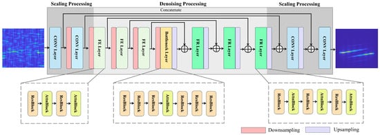
Figure 2. Architecture of the RTDNet denoising backbone.

Table 1. Layer configuration of the RTDNet denoising backbone.

Layers		r	Input Size	${\mathit{C}}_{\mathbf{out}}$	${\mathit{H}}_{\mathbf{out}}\times {\mathit{W}}_{\mathbf{out}}$
Scaling Processing	Conv Layer	1	${256}^2\times 1$	$16C_{in}$	$H_{in}\times W_{in}$
	Downsampling			$C_{in}$	$H_{in}/2\times W_{in}/2$
	Conv Layer		${128}^2\times 16$	$C_{in}$	$H_{in}\times W_{in}$
	Downsampling			$C_{in}$	$H_{in}/2\times W_{in}/2$
Denoising Processing	FE Layer	3	${64}^2\times 16$	$2C_{in}$	$H_{in}\times W_{in}$
	Downsampling			$C_{in}$	$H_{in}/2\times W_{in}/2$
	Bottleneck Layer	1	$8^2\times 128$	$C_{in}$	$H_{in}\times W_{in}$
	Upsampling	3	$8^2\times 128$	$C_{in}$	$H_{in}\times W_{in}$
	FR Layer			$C_{in}/2$	$H_{in}\times W_{in}$
Scaling Processing	Upsampling	1	${64}^2\times 16$	$C_{in}$	$2H_{in}\times 2W_{in}$
	Conv Layer			$C_{in}$	$H_{in}\times W_{in}$
	Upsampling		${128}^2\times 16$	$C_{in}$	$2H_{in}\times 2W_{in}$
	Conv Layer			$C_{in}/16$	$H_{in}\times W_{in}$

3.2. Scaling Processing

RTDNet handles high-resolution TFIs using an encoder-decoder scaling process that first reduces and then restores spatial resolution. In the encoder, strided convolutions progressively downsample the input. Each step begins with a conv-group normalization (GNorm)-sigmoid-weighted linear unit (SiLU) block, which consists of a $3\times 3$ convolution, followed by GNorm [31] and a SiLU activation [32]. After this, a second $3\times 3$ convolution with stride 2 halves the height and width. This downsampling process is repeated twice, as shown in Table 1, producing a hierarchy of feature maps at progressively lower resolution scales. Spatial compression reduces computational cost and enables the network to learn global features, thereby enhancing overall performance.

After denoising, the decoder performs symmetric upsampling to restore the original size. Each upsampling step applies nearest-neighbor interpolation, after which a $3\times 3$ convolution refines the interpolated features, followed by GNorm and SiLU to maintain stable propagation. For every downsampling layer, a corresponding upsampling layer is paired, with skip connections mirroring the path, linking the encoder and decoder at each resolution. In each pair, the encoder feature map is concatenated with the decoder map, restoring high-frequency details lost during compression and preserving precise time-frequency localization. These connections enable the network to reconstruct delicate structures, such as sharp ridges in radar TFIs. Consequently, the scaling stage produces feature maps that integrate global context with recovered details, thereby improving noise cancellation.

3.3. Denoising Processing

RTDNet performs denoising through a sequence of residual and attentional blocks that operate on multiscale feature maps. Each encoder layer, decoder layer, and bottleneck alternates between ResBlock and AttnBlock units to refine features and reduce noise. Figure 3a shows the ResBlock, which comprises two $3\times 3$ convolutions with GNorm and SiLU, along with a residual skip path to facilitate training [33]. ResBlocks extract local features such as edges and ridges while dampening high-frequency noise. Stacking multiple ResBlocks at each scale allows the network to progressively focus on the underlying signal structure.

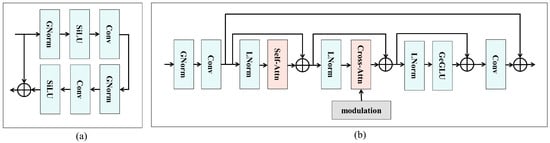
Figure 3. Internal layout of the (a) ResBlock and (b) AttnBlock.

Interleaved with the ResBlocks are AttnBlocks, which provide attention-based feature refinements, as illustrated in Figure 3b. An AttnBlock is a module that applies both self-attention and cross-attention to refine an input feature map in three steps. First, the input is stabilized using GNorm, followed by a $3\times 3$ convolution, then layer normalization (LNorm) [34]. Subsequently, a self-attention mechanism connects the time–frequency patterns dispersed across the TFI. The resulting representation, combined with the residual path, captures long-range dependence while preserving original details. In the second step, cross-attention is performed again using LNorm and modulation embeddings as inputs. Cross-attention injects modulation into the denoising path by directing the features to focus on the modulation class embedding. In the third step, the output is again passed through LNorm and then through the Gaussian error-gated linear unit (GeGLU) [35] feed-forward network to refine the results, allowing the block to highlight signal-consistent responses and suppress residual noise. Finally, a $3\times 3$ convolution is applied, and a residual path is added to preserve the radar structure for downstream analysis. These AttnBlocks are placed throughout the denoising path, enabling the feature maps to effectively incorporate the modulation contexts.

Working in tandem, ResBlocks perform local denoising through convolutional filtering, whereas AttnBlocks enforce global, modulation-aware consistency, thereby preserving overall signal integrity. As features progress through the hierarchy, noise is gradually suppressed, resulting in a clean map ready for reconstruction.

3.4. Attention Mechanism

Figure 4 illustrates the attention operators incorporated in each attention block. Figure 4a depicts self-attention, and Figure 4b shows modulation-conditioned cross-attention [36]. The local feature map is characterized by its height H, width W, and number of channels C. The attention mechanism assigns higher weights to critical information in the signal.

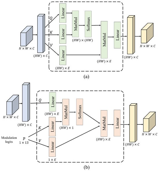
Figure 4. (a) Self-attention and (b) cross-attention operations used in AttnBlock.

3.4.1. Self-Attention

RTDNet employs self-attention in every AttnBlock to capture the global context across the TFI. Before applying attention, the $H\times W\times C$ tensor is reshaped into a sequence of $N=HW$ tokens. Moreover, a flattened input feature map h undergoes linear projections to generate Q (query), K (key), and V (value).

$$Q=W_{Q}h,K=W_{K}h,V=W_{V}h.$$

(4)

Weight matrices $W_Q$, $W_K$, and $W_V$ are learnable parameters that enable the network to extract meaningful features from the input. The output is then obtained as

$$\mathrm{SA}\left(h\right)=softmax\left({\displaystyle \frac{Q{K}^{\top }}{\sqrt{d_k}}}\right)V,$$

(5)

as shown in Figure 4a. The attention output is computed using a scaled dot-product attention mechanism. The relevance between elements in Q and K is calculated and scaled using the square root of the key dimension $\sqrt{d_k}$, followed by a softmax operation. The resulting attention weights are then applied to V to generate the output. This attention mechanism enables the model to learn internal signal patterns and effectively distinguish noise from the signal. In self-attention, each element within the input data interacts with all others, with higher weights assigned to positions that carry greater importance in the signal.

3.4.2. Modulation-Conditioned Cross-Attention

In modulation-conditioned cross-attention, the 13-dimensional logits p (of the recognizer) are fed directly into the denoiser to embed modulation information in every layer. Linear layers map p to the key and value vectors of size E:

$$Q=W_{Q}h,K_{\mathrm{mod}}=W_{K}p,V_{\mathrm{mod}}=W_{V}p,$$

(6)

where $K_{\mathrm{mod}},V_{\mathrm{mod}}\in {\mathbb{R}}^E$. $K_{\mathrm{mod}}$, $V_{\mathrm{mod}}$ are generated from the conditional feature map, which is derived from the modulation information. The cross-attention is then computed as follows:

$$\mathrm{CA}(h,p)=softmax\left({\displaystyle \frac{Q{K}_{\mathrm{mod}}^{\top }}{\sqrt{d_k}}}\right)V_{\mathrm{mod}},$$

(7)

as shown in Figure 4b. In this step, the similarity scores and feature updates are adjusted such that the denoiser focuses on the recognized waveform. Keys and values are derived from the predicted waveform; they inject an inductive bias that directs attention toward the time-frequency patterns characteristic of that modulation while suppressing implausible artifacts [37]. This bias helps RTDNet to reject noise inconsistent with the expected spectrum, even in previously unseen noise conditions.

Self-attention provides RTDNet with long-range reasoning, whereas cross-attention injects waveform-specific priors that guide denoising toward plausible structures. Combined with ResBlock convolutions, these two approaches effectively suppress noise while preserving faint radar signatures, even at very low SNRs.

3.5. Training Objectives

RTDNet is trained in two separate stages rather than a single end-to-end routine.

3.5.1. Modulation Recognition Stage

The ResNet-based classifier was first trained using cross-entropy loss.

$${\mathcal{L}}_{\mathrm{clf}}=-\sum _{j=1}^{13}{y}_{j}log{p}_j,$$

(8)

where $y_j$ denotes the ground truth label for class j, and $p_j$ indicates the softmax probability predicted by the network. The classifier maintained reliable performance even at SNRs as low as $-15$ dB, which is crucial in environments with heavy noise. After convergence, the weights of the classifier were frozen.

3.5.2. Denoising Stage

The denoiser was trained independently using the mean squared error (MSE).

$${\mathcal{L}}_{\mathrm{den}}={\displaystyle \frac{1}{N}}\sum _{i=1}^N{∥{\hat{X}}_i-X_i^{\mathrm{clean}}∥}^2,$$

(9)

where $X_i^{\mathrm{clean}}$ is the clean TFI target and ${\hat{X}}_i$ denotes the denoiser output. During denoiser training, the classifier was bypassed, and ground-truth one-hot logits were fed directly to the denoiser through cross-attention, ensuring the correct modulation context with no backward flow into the classifier.

Decoupled training offers the following three advantages: First, the classifier and denoiser converge independently because their gradients never conflict with those of the other stages. Second, the denoiser receives ground-truth class logits during training, which enables it to learn the correct signal structure for all modulations without distortion. Third, upon inference, the denoiser is fed into the full probability vector from the classifier. Even if the top prediction is incorrect, the soft probabilities continue to guide attention; therefore, the output quality does not collapse and degrades smoothly. Owing to these advantages, the two-stage pipeline maintains high modulation accuracy and preserves key TFI features even at a low SNR, improving the ES performance.

4. Simulation Results

4.1. Dataset and Simulation Setup

Supervised denoising requires noise-free ground-truth references to train the network and evaluate reconstruction accuracy. Since such clean references cannot be obtained from noisy samples, we synthesized a dataset using the simulator and parameters described in [28]. Thirteen LPI radar waveforms, including Rect, LFM, Costas, Barker, Frank, P1–P4, and T1–T4, were simulated at SNR values ranging from $-15$ dB to 0 dB in 1 dB increments. For each waveform-SNR pair, we generated 240 training, 30 validation, and 30 test TFIs, yielding 49,920, 6240, and 6240 samples for the respective splits. Detailed signal parameters are summarized in Table 2, where U denotes a uniform distribution, and $f_s$ represents the sampling frequency. In the simulations, the sampling frequency was set to 100 $\mathrm{MHz}$. The in-phase and quadrature (I/Q) data were transformed into $256\times 256$ TFIs using the CWD. All models were implemented in PyTorch 2.1.0 and trained on an NVIDIA RTX 4060 Ti GPU. Training used the Adam optimizer [38] with an initial learning rate of $1\times {10}^{-3}$, decayed by a factor of 0.1 every 10 epochs, for a total of 30 epochs.

Table 2. Parameters used for signal generation.

Types	Parameters	Range of Value
All	Number of signal samples	512, 1024
	Centre frequency $f_c$ (Hz)	$U(f_s/6,f_s/5)$
	SNR (dB)	$U(-15,0)$
Rect †	–	–
LFM	Bandwidth $\Delta f$ (Hz)	$U(f_s/20,f_s/15)$
Costas	Hopping sequence length	{3, 4, 5, 6}
	Frequency spacing $\Delta f$ (Hz)	$U(f_s/32,f_s/25)$
Barker	Cycles per phase code	{2, 5}
	Barker length	{7, 11, 13}
Frank	Cycles per phase code	{3, 5}
	Number of frequency steps	{6, 7, 8}
P1, P2	Cycles per phase code	{3, 5}
	Number of frequency steps	{6, 8}
P3, P4	Cycles per phase code	{3, 5}
	Number of subcodes in a code	{36, 64}
T1, T2	Number of phase states	2
	Number of segments	{4, 5, 6}
T3, T4	Number of phase states	2
	Bandwidth $\Delta f$ (Hz)	$U(f_s/20,f_s/15)$

† The “Rect” waveform is generated using the global parameters in the “All” row and does not require additional modulation settings.

4.2. Compared Methods

RTDNet, equipped with modulation-conditioned cross-attention, was compared against U2Net, conventional DnCNN and GAN baselines. RTDNet was tested with two recognizer backbones, ResNet-101 and ResNet-34, along with an oracle variant that received the ground-truth modulation label. To ensure a fair comparison, all baseline models were retrained from scratch on the same simulated LPI radar dataset under an identical optimization setup. Specifically, we used the same initial learning rate of $1\times {10}^{-3}$, the same step-decay schedule of 0.1 every 10 epochs, and the Adam optimizer for all models. The denoising loss was MSE for RTDNet, DnCNN, and U2Net, while the GAN baseline was trained with a reconstruction loss based on MSE combined with an adversarial loss term. For stable and fair training across baselines, we allowed up to 50 epochs for all baseline models and applied early stopping with a patience of five based on the validation loss. The best checkpoint selected by early stopping was used for evaluation, ensuring that each baseline was compared at its well-converged operating point rather than being under-trained.

4.3. Modulation Recognition Performance

Figure 5a presents the modulation recognition accuracy of ResNet-101 and ResNet-34 versus SNR. Both backbones achieved at least 95% accuracy for SNRs above $-9$ dB and approached 100% for SNRs above $-4$ dB. Accuracy declined for SNRs below $-10$ dB, particularly for the polyphase and polytime groups, whose stepped or piecewise linear patterns were obscured by the noise floor and became challenging to distinguish. The confusion matrices in Figure 5b,c present the accuracy for each modulation.

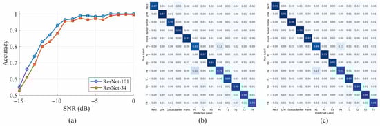
Figure 5. (a) Modulation accuracy versus SNR, (b) confusion matrix for ResNet-34, and (c) confusion matrix for ResNet-101 (darker blue indicates higher normalized proportions).

4.4. Denoising Quality

The three image quality metrics used in this study are defined below for completeness: The first metric, peak signal-to-noise ratio (PSNR), measures restoration quality by comparing a degraded image with a clean image [39]. This provides a quantitative evaluation of the denoising effect.

$$\mathrm{PSNR}=10{log}_{10}\left({\displaystyle \frac{{\mathrm{MAX}}_I^2}{\mathrm{MSE}}}\right),$$

(10)

where ${\mathrm{MAX}}_I$ denotes the maximum possible pixel value, and $\mathrm{MSE}$ is the mean squared error between the denoised output $\hat{X}$ and the clean reference $X^{\mathrm{clean}}$. A higher PSNR corresponds to a lower distortion.

The second metric, intersection over union (IoU), evaluates the extent to which the signal structure is preserved. A threshold is applied to both the label and output to divide the signal-present and signal-absent regions into binary classes, and the IoU is computed as

$$\mathrm{IoU}={\displaystyle \frac{\mathrm{TP}}{\mathrm{TP}+\mathrm{FP}+\mathrm{FN}}}.$$

(11)

This yields the IoU between the predicted signal mask and the ground truth mask, where TP, FP, and FN denote true positives, false positives, and false negatives, respectively.

The structural similarity index measure (SSIM) quantifies perceptual similarity by considering luminance, contrast, and structural consistency [40].

$$\mathrm{SSIM}(x,y)={\displaystyle \frac{(2{\mu }_x{\mu }_y+C_1)(2{\sigma }_{xy}+C_2)}{({\mu }_x^2+{\mu }_y^2+C_1)({\sigma }_x^2+{\sigma }_y^2+C_2)}},$$

(12)

where ${\mu }_x,{\mu }_y$ are the means, ${\sigma }_x^2,{\sigma }_y^2$ are the variances, and ${\sigma }_{xy}$ is the cross covariance of the two images. $C_1$ and $C_2$ are the small stabilizing constants. Values closer to one indicate higher fidelity. Together, PSNR quantifies the overall distortion energy, IoU measures shape retention, and SSIM reflects perceptual quality, providing a balanced picture of denoising performance.

Figure 6 shows the average PSNR, SSIM, and IoU over the 13 waveforms. Across the SNR range, RTDNet with a ResNet backbone outperforms all other models, with ResNet-101 achieving higher performance than ResNet-34. As the SNR increases, RTDNet converges more rapidly toward the Oracle, whereas at lower SNR values its performance approaches that of U2Net. The GAN and DnCNN consistently yield the lowest PSNR, SSIM, and IoU across all SNRs. Table 3 presents a numerical summary of the image quality indicators averaged across the three SNR bands, confirming these trends by separating results into low-, mid-, and high-SNR bands. When the modulation accuracy exceeded 90%, RTDNet was virtually identical to Oracle, with SSIM showing the narrowest gap among all metrics. At the highest SNR, RTDNet-101 and Oracle became almost indistinguishable, confirming that modulation conditioning introduces no performance penalty when the noise is mild.

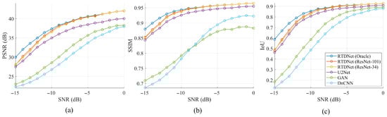
Figure 6. Average denoising performance over 13 modulations: (a) PSNR, (b) SSIM, and (c) IoU.

Table 3. Image-quality metrics averaged by SNR band, where bold and underlined values denote the best and second-best results, respectively.

Model	Low SNR ($-15$ to $-11$ dB)				Mid SNR ($-10$ to $-6$ dB)				High SNR ($-5$ to 0 dB)
	PSNR	IoU	SSIM		PSNR	IoU	SSIM		PSNR	IoU	SSIM
RTDNet (Oracle)	33.39	0.724	0.913		38.87	0.883	0.950		41.34	0.919	0.962
RTDNet (ResNet-101)	31.95	0.661	0.896		38.68	0.879	0.949		41.31	0.918	0.962
RTDNet (ResNet-34)	31.74	0.653	0.894		38.48	0.872	0.948		41.28	0.918	0.961
U2Net [13]	30.76	0.629	0.883		36.71	0.850	0.936		39.33	0.900	0.951
GAN [15]	24.90	0.340	0.738		31.61	0.717	0.827		37.29	0.875	0.881
DnCNN [12]	23.73	0.254	0.716		29.57	0.629	0.831		36.13	0.845	0.914

We further evaluated the robustness of RTDNet under limited training data by reducing the number of training samples to 50%, 25%, and 10% of the original set while keeping the validation and test sets unchanged. To avoid over-representing specific modulation types, the subsets were generated by uniformly subsampling the training data across modulation classes and SNR bins. Figure 7 summarizes the denoising performance for different training ratios. Each reduced-data setting was repeated three times with different random seeds, and the results in Figure 7 are averaged over the three runs. As the training set is reduced, PSNR, SSIM, and IoU consistently decrease, with the largest performance gaps appearing under low-SNR conditions. Nevertheless, even with only 10% of the training data, RTDNet still produces meaningful denoising outputs across the full SNR range, and its performance improves as SNR increases. Notably, using 50% of the training data still yields a solid level of denoising performance, indicating that the proposed approach remains effective under moderately limited training samples.

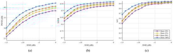
Figure 7. Effect of training sample ratio on average denoising performance: (a) PSNR, (b) SSIM, and (c) IoU.

4.5. Qualitative Comparison

Figure 8 shows six TFIs at $-13$ dB. RTDNet maintains key details, such as Costas hopping slots, Frank stair steps, and thin ridges of polytime signals. In contrast, U2Net blurred several regions, as highlighted by the yellow ellipses in the figure. A closer inspection reveals how the modulation prior guides the restoration implemented by RTDNet.

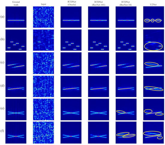
Figure 8. Denoising results of deep learning models at $-13$ dB: (a) Barker, (b) Costas, (c) Frank, (d) P1, (e) T4 with central gaps, and (f) T4 with a continuous ridge.

• Barker and Costas: If the classifier labels the waveform correctly, RTDNet suppresses noise while keeping Barker inter-chip nulls and the Costas hopping grid intact.
• Polyphase: The staircase spectrum of the Frank and P1 codes stays sharp, with noise removed between the steps. This clear preservation of the step pattern indicates that the modulation prior helps the network suppress noise that would otherwise blur the staircase edges.
• Polytime: Under heavy noise, U2Net often confuses these families because their phase patterns are similar to those of LFM and other polyphase codes. The shallow ResNet-34 branch can misclassify and produce the wrong pattern (yellow ellipses), whereas the deeper ResNet-101 branch rarely does so and closely matches the Oracle output.

Overall, the modulation prior enables RTDNet to recover complex waveforms that defeat standard encoder-decoder systems, and the higher recognition accuracy of ResNet-101 directly translates to greater visual fidelity than that of ResNet-34.

We also investigated how RTDNet behaves when the recognizer prediction is incorrect (i.e., top-1 misclassification), since the modulation prior is injected into the denoiser through modulation-conditioned cross-attention. Figure 9 presents two representative low-SNR cases. In Figure 9a, the ground-truth waveform is P2, but the recognizer selects T2 as the top-1 class. In Figure 9b, the ground-truth waveform is T2, but the recognizer selects T4 as the top-1 class. For each case, we compare RTDNet outputs conditioned on the top-1 class, the top-2 class, and the full soft probability vector from the recognizer. When the top-1 class is incorrect, the top-1-conditioned output can inherit artifacts consistent with the mismatched prior, leading to distorted structures, as observed in Figure 9a. However, conditioning on the top-2 class substantially mitigates this distortion when the true waveform is ranked second. Importantly, the soft output produces stable reconstructions that are visually comparable to the best of the top-k-conditioned results in both cases, indicating that cross-attention does not necessarily hallucinate wrong-class features when the predicted probabilities are distributed over multiple plausible classes. Instead, using the full probability vector acts as a mixture prior that improves robustness under misclassification and enables graceful degradation when the recognizer’s confidence is low. However, if the recognizer is highly confident in an incorrect class (i.e., the top-1 probability is very close to 1), the denoiser may inherit a strong but mismatched prior, which can lead to artifacts or distorted structures.

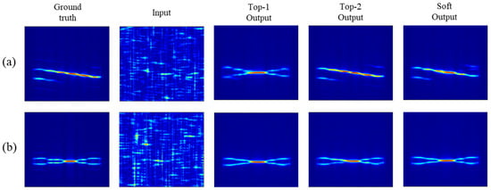
Figure 9. Wrong-prior denoising results at low SNR: (a) P2 misclassified as T2 and (b) T2 misclassified as T4.

We further examined the behavior of RTDNet under out-of-distribution conditions by testing modulation types that were not included in the 13 waveform classes used for training (3rd-order Nonlinear FM (NLFM) and sinusoidal-FM). Figure 10 shows two representative examples at SNR = $-10$ dB and 0 dB, presenting the input TFI, clean ground truth, and RTDNet output. At 0 dB, RTDNet suppresses most of the background noise and recovers the main ridge structure reasonably well, especially for sinusoidal-FM in Figure 10b. However, at $-10$ dB, the outputs exhibit artifacts and shape distortions. For example, Figure 10a shows an extra ridge appearing near the main trajectory, while Figure 10b produces a spurious crossing pattern. This behavior is consistent with the recognize-then-denoise design. The recognizer is a closed-set 13-class classifier and must map an unseen waveform to the nearest in-distribution classes, and the resulting prior is injected through modulation-conditioned cross-attention. When the input SNR is very low, the denoiser relies more on this prior, which can make spurious patterns more likely. In addition, if an unseen waveform has a time–frequency shape similar to one of the trained modulations, the injected prior can bias the output toward that familiar shape–as observed in Figure 10a at 0 dB–leading to distortion. Therefore, RTDNet is primarily intended for closed-set ES operation where the waveform set is known; extending it to robustly handle truly unseen modulations is an important direction for future work, including open-set recognition and uncertainty-aware gating of modulation conditioning.

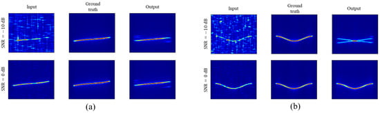
Figure 10. Denoising results on unseen waveforms at $-10$ dB and 0 dB: (a) 3rd-order NLFM and (b) sinusoidal-FM.

4.6. Parameter Estimation Accuracy

Figure 11 shows the root mean square error (RMSE) versus SNR for the time of arrival (TOA), pulse width (PW), carrier frequency ($f_c$), and bandwidth (BW). These parameters were extracted from denoised TFIs using change-point detection with cumulative power ratio (CPD-CP) method [41]. RTDNet with ResNet-101 follows the Oracle line more closely than all the baselines and remains highly robust even at very low SNRs. All conventional baselines deteriorated rapidly as the noise levels increased. Below $-10$ dB, DnCNN exhibits an RMSE that is approximately two to four times higher than RTDNet.

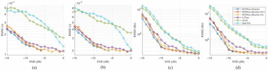
Figure 11. RMSE of parameter estimates versus SNR: (a) TOA, (b) PW, (c) $f_c$, and (d) BW.

Table 4 summarizes the same RMSE averaged over the three SNR bands considered in this study. At low SNR, RTDNet with ResNet-101 recognizer recorded fewer minor errors than U2Net in two of the four parameter estimates. At mid SNR, the same RTDNet led all metrics, yielding lower RMSE than U2Net and the other baselines. At high SNR, the same RTDNet matched the Oracle references, whereas U2Net and the other methods exhibited higher errors. Across all 16 SNR points, the aggregated RMSE of RTDNet with ResNet-101 was approximately 12 % lower than that of U2Net and remained markedly lower than those of the GAN and DnCNN baselines. These results confirm that modulation-aware denoising not only improves the visual quality but also yields more accurate downstream parameter estimates, particularly in the low SNR regime, which is crucial for ES applications.

Table 4. Parameter-estimation RMSE averaged by SNR band, where bold and underlined values denote the best and second-best results, respectively.

Method	Low SNR ($-15$ to $-11$ dB)					Mid SNR ($-10$ to $-6$ dB)					High SNR ($-5$ to 0 dB)
	TOA (µs)	PW (µs)	fc (MHz)	BW (MHz)		TOA (µs)	PW (µs)	fc (MHz)	BW (MHz)		TOA (µs)	PW (µs)	fc (MHz)	BW (MHz)
RTDNet (Oracle)	0.194	0.327	1.867	2.061		0.128	0.216	0.243	0.353		0.113	0.200	0.172	0.301
RTDNet (ResNet-101)	0.217	0.366	2.516	3.167		0.130	0.219	0.246	0.358		0.113	0.200	0.172	0.301
RTDNet (ResNet-34)	0.218	0.362	2.623	3.249		0.132	0.222	0.277	0.424		0.113	0.200	0.172	0.300
U2-Net [13]	0.208	0.356	2.994	3.288		0.143	0.238	0.380	0.618		0.121	0.208	0.183	0.339
GAN [15]	0.471	0.692	6.536	9.781		0.310	0.521	1.036	1.925		0.213	0.411	0.265	0.614
DnCNN [12]	0.441	0.726	8.241	11.886		0.373	0.599	1.039	2.250		0.203	0.335	0.299	0.702

4.7. Post-Denoising Modulation Recognition

Figure 12 and Table 5 illustrate the impact of RTDNet denoising on the classifier.

• High resolution ($256\times 256$): The classification accuracy of the raw TFIs was 89.7%. After denoising, it increased to 90.7% with a gain of 0.99%, which shows that RTDNet causes almost no distortion at a high SNR.
• Moderate downsampling ($128\times 128$ and $64\times 64$): The classification accuracies were 87.5% and 83.7% for raw inputs. Denoising restores 1.65% and 3.77%, respectively, almost matching the full-resolution curve shown in Figure 12.
• Severe downsampling ($32\times 32$): With heavy downsampling, the raw accuracy decreases to 69.5%. Denoising increases this to 80.6% with a gain of 11.17%. Below $-11$ dB, the denoised curve in Figure 12 is up to 22% higher than the raw curve, indicating that RTDNet restores the key features even at a severe resolution.

Figure 12. Effect of denoising on downstream recognition at multiple resolutions.

Table 5. Classification accuracy before and after denoising.

Input Size	Raw (%)	Denoised (%)	Gain (%)
32 × 32	69.46	80.63	11.17
64 × 64	83.70	87.47	3.77
128 × 128	87.53	89.18	1.65
256 × 256	89.73	90.72	0.99

Table 5. Classification accuracy before and after denoising.

Input Size	Raw (%)	Denoised (%)	Gain (%)
32 × 32	69.46	80.63	11.17
64 × 64	83.70	87.47	3.77
128 × 128	87.53	89.18	1.65
256 × 256	89.73	90.72	0.99

4.8. Ablation on Modulation Prior

Figure 13 shows four variants at $-12$ dB: Oracle, RTDNet with ResNet-101, RTDNet with ResNet-34, and a version without cross-attention (w/o-CA).

• Image quality, Figure 13a–c: When cross-attention is removed (w/o-CA), all three metrics-PSNR, SSIM, and IoU-drop noticeably, confirming that modulation guidance is crucial for high-fidelity restoration. Switching from the lighter ResNet-34 to the deeper ResNet-101 recognizer yields a further, albeit modest, uplift, illustrating that superior classification still translates into cleaner reconstructions.
• Parameter RMSE, Figure 13d–g: Without cross-attention, the bandwidth error rises sharply, and the other three parameters also become worse, underscoring the importance of modulation conditioning for accurate parameter recovery. Replacing ResNet-34 with ResNet-101 consistently lowers every RMSE bar and brings RTDNet closer to the Oracle ceiling, showing that higher recognizer accuracy directly benefits downstream estimation.

Overall, the ablation confirmed these two trends: (i) Modulation-aware cross-attention is indispensable, and (ii) the better the recognizer, the closer RTDNet approaches the Oracle ceiling.

Figure 13. Ablation results at $-12$ dB: (a) PSNR, (b) IoU, (c) SSIM, (d) TOA RMSE, (e) PW RMSE, (f) $f_c$ RMSE, and (g) BW RMSE.

4.9. Model Efficiency and Resource Utilization

Table 6 compares the model size, computational cost, and measured inference latency for a single $256\times 256$ TFI. Inference time was measured on an NVIDIA RTX 4060 Ti GPU by running 100 samples with a batch size of 1. RTDNet achieved an average latency of 32.41 ms per image. RTDNet contains only 5.6 M parameters and requires 7.72 GFLOPs, which is approximately one-tenth the parameter count of U2Net (44.01 M, 75.3 GFLOPs) and far lower FLOPs than the GAN baseline (160.72 GFLOPs). Although RTDNet shows a longer latency than some baselines in our current implementation, this suggests that factors beyond FLOPs, such as memory traffic and kernel overhead, can significantly affect runtime. Importantly, RTDNet delivers the best performance for every accuracy metric reported earlier, providing a favorable accuracy-efficiency trade-off for ES applications.

Table 6. Model size, computational cost, and inference latency per $256\times 256$ TFI.

Method	Parameters	FLOPs	Avg Latency (ms)
RTDNet	5.6 M	7.72 G	32.41
U2Net [13]	44.01 M	75.3 G	14.27
GAN [15]	1.22 M	160.72 G	16.52
DnCNN [12]	556.03 k	73.14 G	5.97

5. Conclusions

This paper introduced RTDNet, which combines modulation-aware cross-attention with a lightweight encoder–decoder backbone to restore LPI radar signals. By first classifying the waveform and passing the resulting logits to the denoiser, RTDNet directs its attention toward modulation-consistent structures, suppressing the spurious components that conventional filtering leaves behind. Simulation-based performance analysis across the full SNR range from $-15$ dB to 0 dB shows that RTDNet outperforms existing techniques in terms of PSNR, SSIM, and IoU. It also achieves the lowest RMSE in TOA, PW, $f_c$, and BW estimation. Significantly, RTDNet delivers these performance gains with a compact model size and low computational complexity, facilitating its practical deployment for real-time processing in resource-constrained electronic warfare systems. Visual examples further demonstrate that RTDNet retains key details, such as Costas slots, Frank steps, and thin ridges of polytime codes, even under the worst SNR conditions, whereas other methods blur or erase these features. Overall, these results indicate that modulation-conditioned attention can achieve strong denoising while faithfully retaining essential signal features, thereby offering a practical path toward more intelligent and resilient EW receivers.

In practical ES environments, however, interference may be non-Gaussian and structured, and can overlap with the desired LPI waveform patterns. Although the attention mechanism and modulation-conditioned priors can help suppress components that are inconsistent with expected waveform structures, performance may degrade when interference exhibits signal-like patterns or when noise statistics differ from the training distribution. Future work will focus on extending RTDNet to handle non-Gaussian noise and structured interference by augmenting the training data with diverse noise models, adding robustness-promoting loss terms, and introducing uncertainty-aware conditioning. Additionally, we will explore inference-time optimizations to reduce latency.

6. DURC Statement

Current research is limited to radar signal processing for denoising and parameter estimation using simulated data, which is beneficial for improving the robustness and reliability of signal analysis in low-SNR environments and does not pose a threat to public health or national security. The authors acknowledge the potential dual-use implications of radar-related signal processing techniques and confirm that all necessary precautions have been taken to prevent potential misuse. In particular, this manuscript does not provide operational guidance, deployment procedures, or sensitive system-level specifications intended for military use. As an ethical responsibility, the authors strictly adhere to relevant national and international laws and ethical standards regarding dual-use research of concern (DURC). The authors advocate responsible deployment, ethical considerations, regulatory compliance, and transparent reporting to mitigate misuse risks and foster beneficial outcomes.

References

- Gupta, M.; Hareesh, G.; Mahla, A.K. Electronic warfare: Issues and challenges for emitter classification. Def. Sci. J. 2011, 61, 467–472. [Google Scholar] [CrossRef]
- Adamy, D. EW 101: A First Course in Electronic Warfare; Artech House: Norwood, MA, USA, 2001; Volume 101. [Google Scholar]
- Pace, P.E. Detecting and Classifying Low Probability of Intercept Radar; Artech House: Norwood, MA, USA, 2004. [Google Scholar]
- Schleher, D.C. LPI radar: Fact or fiction. IEEE Aerosp. Electron. Syst. Mag. 2006, 21, 3–6. [Google Scholar] [CrossRef]
- Chang, S.; Tang, S.; Deng, Y.; Zhang, H.; Liu, D.; Wang, W. An Advanced Scheme for Deceptive Jammer Localization and Suppression in Elevation Multichannel SAR for Underdetermined Scenarios. IEEE Trans. Aerosp. Electron. Syst. 2025; early access. [Google Scholar] [CrossRef]
- Wang, W.; Wu, J.; Pei, J.; Sun, Z.; Yang, J. Deception-Jamming Localization and Suppression via Configuration Optimization for Multistatic SAR. IEEE Trans. Geosci. Remote Sens. 2022, 60, 1–16. [Google Scholar] [CrossRef]
- Tang, J.; Yang, Z.; Cai, Y. Wideband passive radar target detection and parameters estimation using wavelets. In Proceedings of the IEEE International Radar Conference, Alexandria, VA, USA, 7–12 May 2000; pp. 815–818. [Google Scholar]
- Shin, J.-W.; Song, K.-H.; Yoon, K.-S.; Kim, H.-N. Weak radar signal detection based on variable band selection. IEEE Trans. Aerosp. Electron. Syst. 2016, 52, 1743–1755. [Google Scholar] [CrossRef]
- Wu, Z.; Huang, N.E. Ensemble empirical mode decomposition: A noise-assisted data analysis method. Adv. Adapt. Data Anal. 2009, 1, 1–41. [Google Scholar] [CrossRef]
- Qi, T.; Wei, X.; Feng, G.; Zhang, F.; Zhao, D.; Guo, J. A method for reducing transient electromagnetic noise: Combination of variational mode decomposition and wavelet denoising algorithm. Measurement 2022, 198, 111420. [Google Scholar] [CrossRef]
- Jiang, M.; Zhou, F.; Shen, L.; Wang, X.; Quan, D.; Jin, N. Multilayer decomposition denoising empowered CNN for radar signal modulation recognition. IEEE Access 2024, 12, 31652–31661. [Google Scholar] [CrossRef]
- Zhang, K.; Zuo, W.; Chen, Y.; Meng, D.; Zhang, L. Beyond a Gaussian denoiser: Residual learning of deep CNN for image denoising. IEEE Trans. Image Process. 2017, 26, 3142–3155. [Google Scholar] [CrossRef]
- Lee, S.; Nam, H. LPI radar signal recognition with U2-Net-based denoising. In Proceedings of the 14th International Conference on Information and Communication Technology Convergence (ICTC), Jeju, Republic of Korea, 11–13 October 2023; pp. 1721–1724. [Google Scholar]
- Qin, X.; Zhang, Z.; Huang, C.; Dehghan, M.; Zaiane, O.R.; Jagersand, M. U2-Net: Going deeper with nested U-structure for salient object detection. Pattern Recognit. 2020, 106, 107404. [Google Scholar] [CrossRef]
- Jiang, W.; Li, Y.; Tian, Z. LPI radar signal enhancement based on generative adversarial networks under small samples. In Proceedings of the IEEE 6th International Conference on Computer and Communications (ICCC), Chengdu, China, 11–14 December 2020; pp. 1314–1318. [Google Scholar]
- Goodfellow, I.; Pouget-Abadie, J.; Mirza, M.; Xu, B.; Warde-Farley, D.; Ozair, S.; Courville, A.; Bengio, Y. Generative adversarial networks. Commun. ACM 2020, 63, 139–144. [Google Scholar] [CrossRef]
- Krull, A.; Buchholz, T.-O.; Jug, F. Noise2Void–Learning denoising from single noisy images. In Proceedings of the IEEE/CVF Conference on Computer Vision and Pattern Recognition (CVPR), Long Beach, CA, USA, 15–20 June 2019; pp. 2129–2137. [Google Scholar]
- Batson, J.; Royer, L. Noise2Self: Blind denoising by self-supervision. In Proceedings of the 36th International Conference on Machine Learning (ICML), Long Beach, CA, USA, 9–15 June 2019; Volume 97, pp. 524–533. [Google Scholar]
- Liao, Y.; Wang, X.; Jiang, F. LPI radar waveform recognition based on semi-supervised model all mean teacher. Digit. Signal Process. 2024, 151, 104568. [Google Scholar] [CrossRef]
- Huang, C.; Xu, X.; Fan, F.; Wei, S.; Zhang, X.; Liu, D.; Gu, M. A low-SNR-adaptive temporal network with smart mask attention for radar signal modulation recognition. Digit. Signal Process. 2025, 168, 105640. [Google Scholar] [CrossRef]
- Xu, S.; Liu, L.; Zhao, Z. Unsupervised recognition of radar signals combining multi-block TFR with subspace clustering. Digit. Signal Process. 2024, 151, 104552. [Google Scholar] [CrossRef]
- Cai, J.; Gan, F.; Cao, X.; Liu, W.; Li, P. Radar intra-pulse signal modulation classification with contrastive learning. Remote Sens. 2022, 14, 5728. [Google Scholar] [CrossRef]
- Chen, K.; Zhang, J.; Chen, S.; Zhang, S.; Zhao, H. Automatic modulation classification of radar signals utilizing X-Net. Digit. Signal Process. 2022, 123, 103396. [Google Scholar] [CrossRef]
- Liang, J.; Luo, Z.; Liao, R. Intra-pulse modulation recognition of radar signals based on efficient cross-scale aware network. Sensors 2024, 24, 5344. [Google Scholar] [CrossRef]
- Bhatti, S.G.; Taj, I.A.; Ullah, M.; Bhatti, A.I. Transformer-based models for intrapulse modulation recognition of radar waveforms. Eng. Appl. Artif. Intell. 2024, 136, 108989. [Google Scholar] [CrossRef]
- Wu, C.; Chen, S.; Sun, G. Automatic modulation recognition framework for LPI radar based on CNN and Vision Transformer. In Proceedings of the 2024 8th International Conference on Computer Science and Artificial Intelligence, Beijing, China, 6–8 December 2024. [Google Scholar]
- Qi, Y.; Ni, L.; Feng, X.; Li, H.; Zhao, Y. LPI radar waveform modulation recognition based on improved EfficientNet. Electronics 2025, 14, 4214. [Google Scholar] [CrossRef]
- Huynh-The, T.; Doan, V.S.; Hua, C.H.; Pham, Q.V.; Nguyen, T.V.; Kim, D.S. Accurate LPI radar waveform recognition with CWD-TFA for deep convolutional network. IEEE Wirel. Commun. Lett. 2021, 10, 1638–1642. [Google Scholar] [CrossRef]
- Kong, S.H.; Kim, M.; Hoang, L.M.; Kim, E. Automatic LPI radar waveform recognition using CNN. IEEE Access 2018, 6, 4207–4219. [Google Scholar] [CrossRef]
- Choi, H.-I.; Williams, W.J. Improved time-frequency representation of multicomponent signals using exponential kernels. IEEE Trans. Acoust. Speech Signal Process. 1989, 37, 862–871. [Google Scholar] [CrossRef]
- Wu, Y.; He, K. Group normalization. In Proceedings of the European Conference on Computer Vision (ECCV), Munich, Germany, 8–14 September 2018; pp. 3–19. [Google Scholar]
- Elfwing, S.; Uchibe, E.; Doya, K. Sigmoid-weighted linear units for neural network function approximation in reinforcement learning. Neural Netw. 2018, 107, 3–11. [Google Scholar] [CrossRef] [PubMed]
- He, K.; Zhang, X.; Ren, S.; Sun, J. Deep residual learning for image recognition. In Proceedings of the IEEE Conference on Computer Vision and Pattern Recognition (CVPR), Las Vegas, NV, USA, 27–30 June 2016; pp. 770–778. [Google Scholar]
- Ba, J.L.; Kiros, J.R.; Hinton, G.E. Layer normalization. arXiv 2016, arXiv:1607.06450. [Google Scholar] [CrossRef]
- Shazeer, N. GLU variants improve transformer. arXiv 2020, arXiv:2002.05202. [Google Scholar] [CrossRef]
- Vaswani, A.; Shazeer, N.; Parmar, N.; Uszkoreit, J.; Jones, L.; Gomez, A.N.; Kaiser, Ł.; Polosukhin, I. Attention is all you need. In Advances in Neural Information Processing Systems; Curran Associates Inc.: Red Hook, NY, USA, 2017; Volume 30, pp. 5998–6008. [Google Scholar]
- Yang, T.; Lan, C.; Lu, Y. Diffusion model with cross attention as an inductive bias for disentanglement. Adv. Neural Inf. Process. Syst. 2024, 37, 82465–82492. [Google Scholar]
- Kingma, D.P.; Ba, J. Adam: A method for stochastic optimization. In Proceedings of the 3rd International Conference on Learning Representations (ICLR), San Diego, CA, USA, 7–9 May 2015. [Google Scholar]
- Ward, C.M.; Harguess, J.; Crabb, B.; Parameswaran, S. Image quality assessment for determining efficacy and limitations of super-resolution convolutional neural network (SRCNN). In Applications of Digital Image Processing XL; SPIE: Bellingham, WA, USA, 2017; Volume 10396. [Google Scholar]
- Wang, Z.; Bovik, A.C.; Sheikh, H.R.; Simoncelli, E.P. Image quality assessment: From error visibility to structural similarity. IEEE Trans. Image Process. 2004, 13, 600–612. [Google Scholar] [CrossRef]
- Bang, J.-H.; Park, D.-H.; Lee, W.; Kim, D.; Kim, H.-N. Accurate estimation of LPI radar pulse train parameters via change point detection. IEEE Access 2023, 11, 12796–12807. [Google Scholar] [CrossRef]
Disclaimer/Publisher’s Note: The statements, opinions and data contained in all publications are solely those of the individual author(s) and contributor(s) and not of MDPI and/or the editor(s). MDPI and/or the editor(s) disclaim responsibility for any injury to people or property resulting from any ideas, methods, instructions or products referred to in the content. |
© 2026 by the authors. Licensee MDPI, Basel, Switzerland. This article is an open access article distributed under the terms and conditions of the Creative Commons Attribution (CC BY) license.