State of Charge (SoC) Estimation with Electrochemical Impedance Spectroscopy (EIS) Data Using Different Ensemble Machine Learning Algorithms

Abstract

Accurate state of charge (SoC) estimation is critical for the safety, performance, and longevity of lithium-ion batteries in electric vehicles and energy storage systems. This study investigates the application of Electrochemical Impedance Spectroscopy (EIS) data in conjunction with tree-based ensemble machine learning algorithms—Random Forest, Extra Trees, Gradient Boosting, XGBoost, and AdaBoost—for precise SoC prediction. A real dataset comprising multi-frequency EIS measurements was used to train and evaluate the models. The models’ performances were assessed using Mean Squared Error (MSE), Root Mean Squared Error (RMSE), and the coefficient of determination (R²). The results show that Extra Trees achieved the best accuracy (MSE = 1.76, RMSE = 1.33, R² = 0.9977), followed closely by Random Forest, Gradient Boosting, and XGBoost, all maintaining RMSE values below 1.6% SoC. Predictions from these models closely matched the ideal 1:1 relationship, with tightly clustered error distributions indicating minimal bias. AdaBoost returned a higher RMSE (3.06% SoC) and a broader error spread. These findings demonstrate that tree-based ensemble models, particularly Extra Trees and Random Forest, offer robust, high-accuracy solutions for EIS-based SoC estimation, making them promising candidates for integration into advanced battery management systems.

1. Introduction

Accurate estimation of a battery’s state of charge (SoC) is a critical function in battery management systems for lithium-ion batteries [1], especially for electric vehicles. SoC represents the remaining capacity of the battery as a percentage of its full charge and knowing it precisely helps prevent overcharging or deep discharging, which can otherwise degrade battery performance and longevity [1,2]. In electric vehicles (EVs) and other energy storage applications, reliable SoC information is essential for safety, optimizing performance, and providing accurate range or runtime predictions [1,3,4,5]. Traditionally, SoC estimation is achieved through methods such as coulomb counting, tracking charge inflow/outflow, open-circuit voltage correlation, or model-based observers, e.g., Kalman filters that use equivalent-circuit or electrochemical models. However, direct measurement of SoC is not possible in practice—no sensor directly reads the “remaining charge” outside of lab techniques [6]. Model-based methods require extensive knowledge of the battery’s internal behavior and can become inaccurate due to model mismatch, parameter drift with aging, and measurement noise. This motivates the exploration of data-driven approaches that can learn the SoC relationship from data without needing a perfect physical model [7]. In fact, with the greater availability of battery data and improved computing power, machine learning (ML) methods are increasingly being investigated for SoC and state-of-health estimation [3]. Among advanced diagnostic techniques for batteries, Electrochemical Impedance Spectroscopy (EIS) stands out as a rich source of information about the cell’s internal state [8,9]. EIS involves applying small sinusoidal perturbations over a range of frequencies and measuring the battery’s complex impedance response [2]. The impedance spectrum captures electrochemical processes (charge-transfer resistance, double-layer capacitance, diffusion processes, etc.) that change with the battery’s state of charge.

Notably, impedance spectra are highly sensitive to SoC—the shape and magnitude of the EIS response vary with the amount of charge in the cell [10]. Prior studies have used EIS data to assess both SoC and state-of-health (SoH) of batteries, demonstrating that different SoC levels produce distinguishable impedance signatures [2]. For example, the Nyquist plot of impedance (imaginary vs. real part) will shift its characteristic semicircles and line segments as SoC changes. However, translating an impedance spectrum into an exact SoC value is non-trivial, since the relationship is complex and multi-dimensional [10,11]. This is where machine learning can be potent: rather than explicitly modeling the electrochemical phenomena, ML models can be trained to recognize patterns in the EIS data that correspond to known SoC values.

Concept of EIS

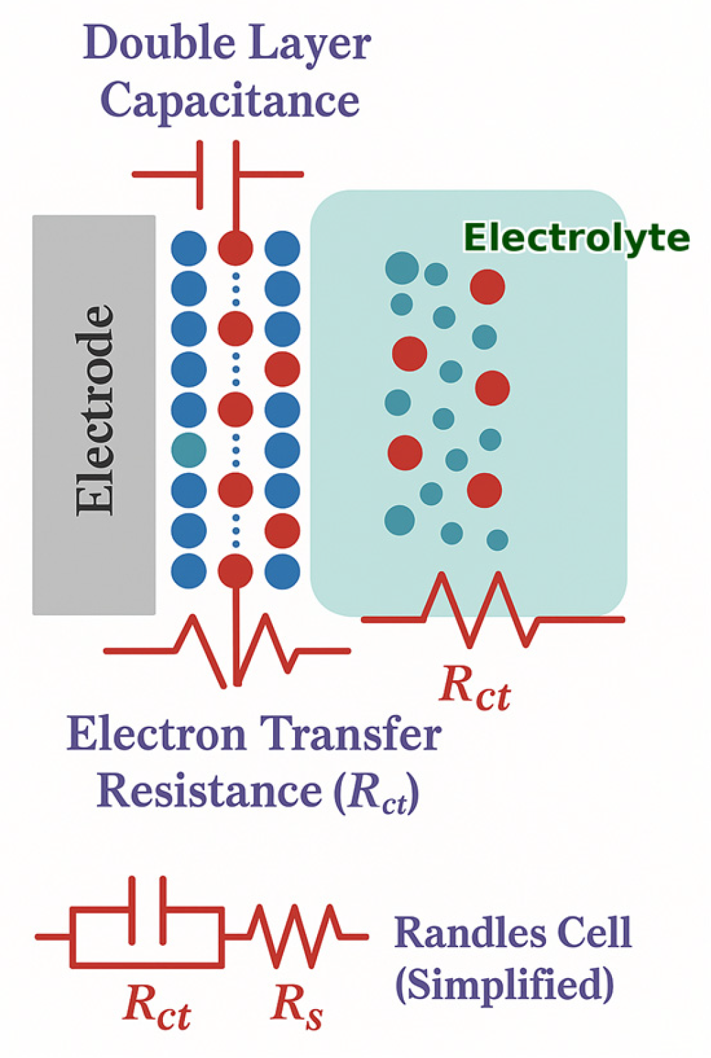
Electrochemical Impedance Spectroscopy (EIS) is a powerful diagnostic technique used to study the dynamic response of electrochemical systems by applying a small-amplitude sinusoidal voltage signal over a range of frequencies and measuring the resulting current [12]. This approach allows for the separation of resistive and capacitive contributions to the system’s overall impedance, providing valuable insights into processes such as charge-transfer, double-layer formation, and ion diffusion [13]. By analyzing the relationship between the applied signal and the system’s phase-shifted current response, EIS enables the modeling of electrochemical behavior using equivalent circuits that can be directly linked to physical and chemical processes within the system [12]. Figure 1 depicts a typical EIS process for a conventional electrochemical cell, in which redox species from the electrodes interact in the electrolyte. This process comprises charge-transfer from the bulk solution to the electrode surface, along with electrolyte resistance. Each of these features can be represented by an equivalent electrical circuit containing resistors, capacitors, or constant-phase elements, arranged in series or parallel configurations.

Figure 1. A simplified schematic describing the EIS circuit and the redox reaction taking place at the surface of working electrodes in a conventional electrochemical cell. $R_{ct}$ represents the charge-transfer resistance, $R_S$ is electrolyte resistance, and $C_{dl}$ is double-layer capacitance.

A small-signal sinusoidal current perturbation is applied to the cell over a set of angular frequencies ω = 2πf, and the complex impedance can be measured as follows:

$$\mathit{Z}\left(\mathit{\omega }\right)=\mathit{V}\left(\mathit{\omega }\right)/\mathit{I}\left(\mathit{\omega }\right)=\mathit{R}\left(\mathit{\omega }\right)+\mathit{j}\mathit{X}\left(\mathit{\omega }\right)$$

(1)

The magnitude and phase are given as

$$\left|\mathit{Z}\right|=\surd ({\mathit{R}}^2+{\mathit{X}}^2) \mathit{a}\mathit{n}\mathit{d} \mathit{\angle }\mathit{Z}=\mathit{a}\mathit{r}\mathit{c}\mathit{t}\mathit{a}\mathit{n}(\mathit{X}/\mathit{R})$$

(2)

The coordinate conventions used are Nyquist $\left(Re\right\{Z\}, -Im\{Z\left\}\right)$, and Bode $\left|Z\right|\left(f\right)$ and $\angle Z\left(f\right)$ against ${log}_{10}\left(f\right).$ In practice, SoC sensitivity is concentrated in mid- to low-frequency bands that capture charge-transfer and diffusion phenomena.

In the literature, a broad spectrum of SoC estimators exists: SoC look-up table, open-circuit-voltage (OCV) methods, Kalman filter and other model-based estimators, EIS data-driven approaches, and more [14,15,16,17]. OCV methods rely on a calibrated OCV–SoC map and can be highly accurate at equilibrium; however, they require long rest periods to suppress polarization, are sensitive to temperature and aging drift, and suffer from hysteresis in many chemistries, which limits real-time applicability under dynamic loads. Kalman filter-based estimators (e.g., EKF/UKF/dual-KF) fuse current/voltage measurements with a cell model (OCV–SoC map + RC) to estimate SoC online; they work well when model parameters and OCV tables are identified and tracked, but accuracy can degrade with model mismatch, parameter drift, and cell-to-cell variability unless frequent re-identification is performed. In contrast, Electrochemical Impedance Spectroscopy (EIS) provides a short, quasi-stationary snapshot of the cell’s frequency response from which ohmic, charge-transfer, and diffusion features can be extracted; these features are informative for SoC [10,18].

2. Methodology and Algorithms

2.1. Motivation

Using EIS impedance spectrum data with data-driven ML algorithms, we aim to improve SoC estimation accuracy beyond what is possible with other methods. EIS-based estimation could complement or enhance existing methods, potentially enabling SoC determination even when voltage or current measurements are not informative (e.g., in flat regions of the voltage–SOC curve or under varying temperature conditions). In this work, we present a comparative evaluation of several machine learning algorithms for SoC estimation using EIS data [19]. We used a recently published EIS dataset for lithium-ion batteries and trained five different regression models to predict SoC from the impedance spectra. The algorithms include both simple and advanced methods: Random Forest, Gradient Boosting, XGBoost, AdaBoost, and Extra Trees. We discuss the justification for each model, their suitability for the task, and compare their performance on a common dataset. The results highlight the advantages of certain models in capturing the complex EIS–SoC relationship and underscore important considerations in generalization and robustness of the estimation.

2.2. Data Acquisition

The study utilizes a comprehensive EIS dataset collected from lithium-ion cells (Lithium Iron Phosphate chemistry) at various states of charge [19]. In the dataset, impedance spectroscopy was performed on 11 brand-new 600 mAh cylindrical LiFePO₄ cells at SoC levels of 100%, 95%, 90%, 85%, … down to 5% (in 5% increments) (see Table 1 for typical EIS CSV data for 5% SOC); this same kind of file is replicated for different SOCs at various frequency points between 0.01 and 1000 Hz. The EIS was conducted across a broad frequency range, from approximately 0.01 Hz up to 1 kHz, yielding an impedance spectrum at around 28 distinct frequency points for each SoC point [19]. The raw data thus consists of the real and imaginary parts of impedance at each frequency, along with the known SoC label for that spectrum. Before applying machine learning, basic preprocessing steps were carried out. Each impedance spectrum was converted into a feature vector; in our approach, we used the real and imaginary components at each frequency to calculate the magnitude and phase so that each sample is represented by a fixed-length feature vector capturing the spectral shape. We then normalized the features to ensure that all frequency components were on a comparable scale for algorithms sensitive to feature scaling. State of charge labels used throughout this study are tied to a constant current discharge calibration performed with the ZKETECH EBD A20H EB tester. Table 2 summarizes the discharge settings, current and cut-off voltage, and the resulting capacity for the LFP cell set used in the EIS measurements.

Table 1. EIS CSV data at 5% SOC at various frequency points 0.01 to 1000 Hz (each file represents one measurement at a specific SOC (5%, 10%, 15%, 20%, … 100%)) [19].

Frequency (Hz)	R (Ohm)	X (Ohm)	V (V)	T (Deg C)	Range (Ohm)
0.01	0.182033	−0.10447	3.09408	20	0.3
0.02	0.153463	−0.07256	3.10256	20	0.3
0.03	0.141077	−0.05803	3.10426	20	0.3
0.05	0.129268	−0.044	3.10564	20	0.3
0.08	0.120899	−0.0346	3.1064	20	0.3
0.1	0.117482	−0.03102	3.10687	20	0.3
0.2	0.10866	−0.02273	3.10731	20	0.3
… 1000	0.059685	−0.00444	3.10814	20	0.3

Table 2. Constant current discharging and capacity calibration of the cell using the battery EB tester [19].

Time (S)	Cur (A)	Vol (V)	EB Tester Software
0	0	3.329	Device: ZKETECH EBD A20H
0	0	3.329	Mode:D-CC 0.12 A 2.00 V
1	0.12	3.32	Begin Volt: 3.329 V
3	0.12	3.315	Cutoff Volt: 1.998 V
5	0.12	3.315	Capacity: 633 mAh
7	0.12	3.315	Energy: 2036 mWh
9	0.12	3.314	Avg Volt: 3.22 V
11	0.12	3.313	Title: EB Tester Software
13	0.12	3.309	www.zketech.com
15	0.12	3.308
17	0.12	3.308
… 18,977	0.12	1.998

Impedance spectrum data can be numerically computed using the Kramers–Kronig relations. These relations allow for the determination of the real component of the impedance spectrum from its imaginary counterpart, and vice versa, providing a consistency check for the electrochemical impedance data.

$${\mathit{Z}}^{\prime }\left(\mathit{\omega }\right)={\mathit{R}}_{\mathbf{\infty }}+{\displaystyle \frac{2}{\mathit{\pi }}}{\int }_0^{\mathbf{\infty }}{\displaystyle \frac{\mathit{x}{\mathit{Z}}^{″}\left(\mathit{x}\right)-\mathit{\omega }{\mathit{Z}}^{″}\left(\mathit{\omega }\right)}{{\mathit{x}}^2-{\mathit{\omega }}^2}}\mathit{d}\mathit{x}$$

(3)

$${\mathit{Z}}^{″}(\mathit{\omega })={\displaystyle \frac{2\mathit{\omega }}{\mathit{\pi }}}{\int }_0^{\mathit{\infty }}{\displaystyle \frac{{\mathit{Z}}^{\prime }\left(\mathit{x}\right)-{\mathit{Z}}^{\prime }\left(\mathit{\omega }\right)}{{\mathit{x}}^2-{\mathit{\omega }}^2}}\mathit{d}\mathit{x}$$

(4)

• where
• Z′(ω) = Real part of the impedance at angular frequency (ω).
• Z′′(ω) = Imaginary part of impedance at angular frequency (ω).
• ω = Angular frequency of interest.
• x = Dummy variable of integration representing angular frequency (rad/s).
• R∞ = Resistance at infinite frequency (intercept on real axis of Nyquist plot).
• Π = Constant pi, approximately 3.14159.

The dataset was split into a training set for model fitting and a test set for evaluating performance on unseen data. The learning task is formulated as a regression: the models take the EIS feature vector as input and output a predicted SoC (in %). We selected Root Mean Squared Error (RMSE) as the primary training loss and Mean Squared Error (MSE), and R² (coefficient of determination) as additional performance metrics to assess the machine learning algorithms’ performance.

$$\mathit{M}\mathit{S}\mathit{E}={\displaystyle \frac{1}{\mathit{n}}}{\sum }_{\mathit{i}=1}^{\mathit{n}}{({\mathit{y}}_{\mathit{i}}-{\hat{\mathit{y}}}_{\mathit{i}})}^2$$

(5)

$$\mathit{R}\mathit{M}\mathit{S}\mathit{E}=\sqrt{\mathit{M}\mathit{S}\mathit{E}}=\sqrt{{\displaystyle \frac{1}{\mathit{n}}}{\sum }_{\mathit{i}=1}^{\mathit{n}}{({\mathit{y}}_{\mathit{i}}-{\hat{\mathit{y}}}_{\mathit{i}})}^2}$$

(6)

$${\mathbf{R}}^2=1-{\displaystyle \frac{\sum _{\mathbf{i}=1}^{\mathbf{n}}{({\mathbf{y}}_{\mathbf{i}}-{\hat{\mathbf{y}}}_{\mathbf{i}})}^2}{\sum _{\mathbf{i}=1}^{\mathbf{n}}{({\mathbf{y}}_{\mathbf{i}}-\overline{\mathbf{y}})}^2}}$$

(7)

• where ${\mathit{R}}^2\in \left[-\mathit{\infty },1\right]$
• $\mathrm{n}=\text{Number of data points}$
• ${\mathrm{y}}_{\mathrm{i}}=\text{Actual (true) value}$
• ${\hat{\mathrm{y}}}_{\mathrm{i}}=\text{Predicted value}$
• $\overline{\mathrm{y}}=\text{Mean of the actual values}$
• $({\mathrm{R}}^2=1):\text{perfect prediction}$
• $({\mathrm{R}}^2=0):\text{model does no better than the mean}$
• $({\mathrm{R}}^2<0):\text{model is worse than just predicting the mean}$

2.3. Nyquist and Bode Plots for Lithium-Ion Cells at Various States of Charge

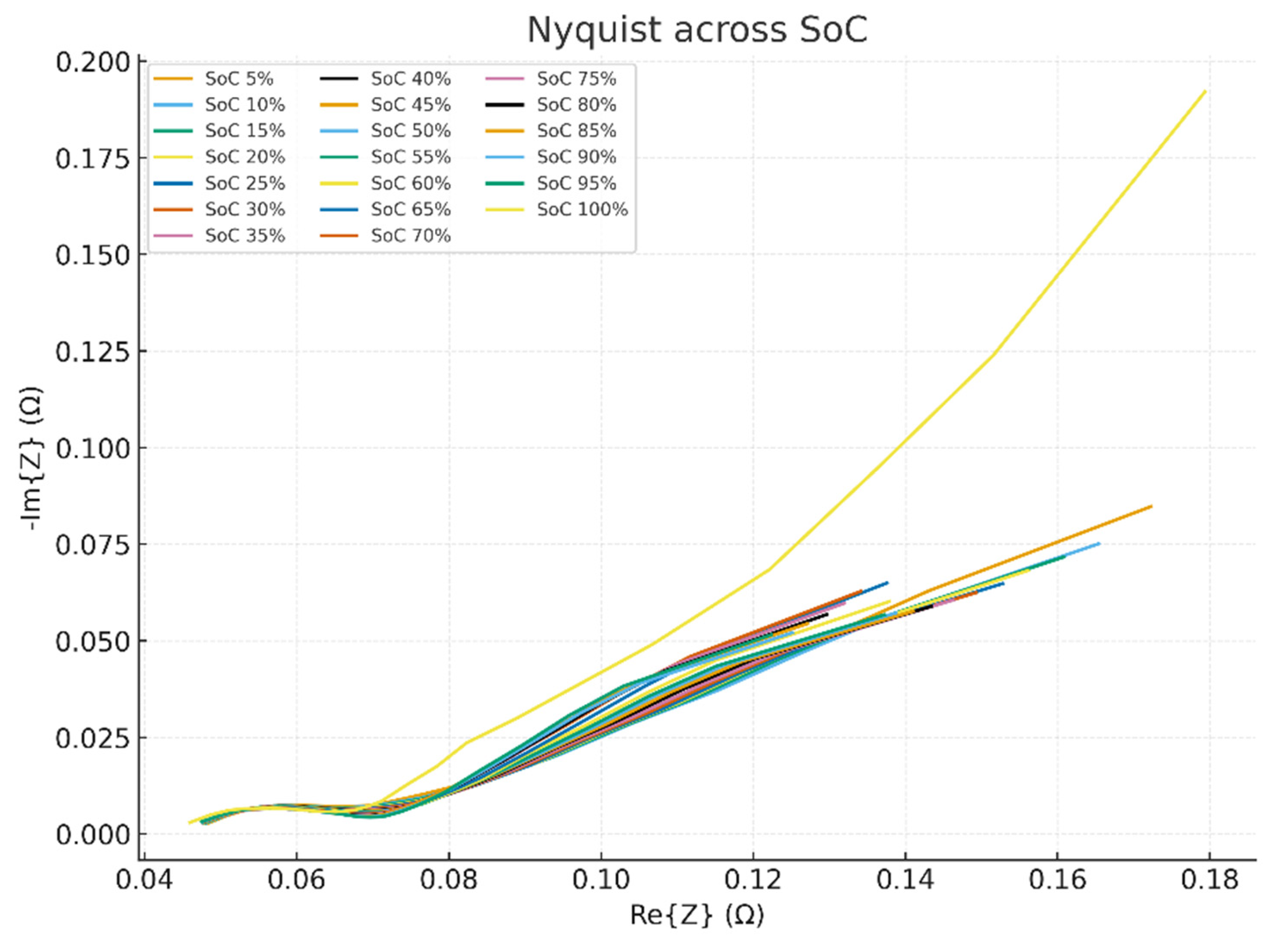
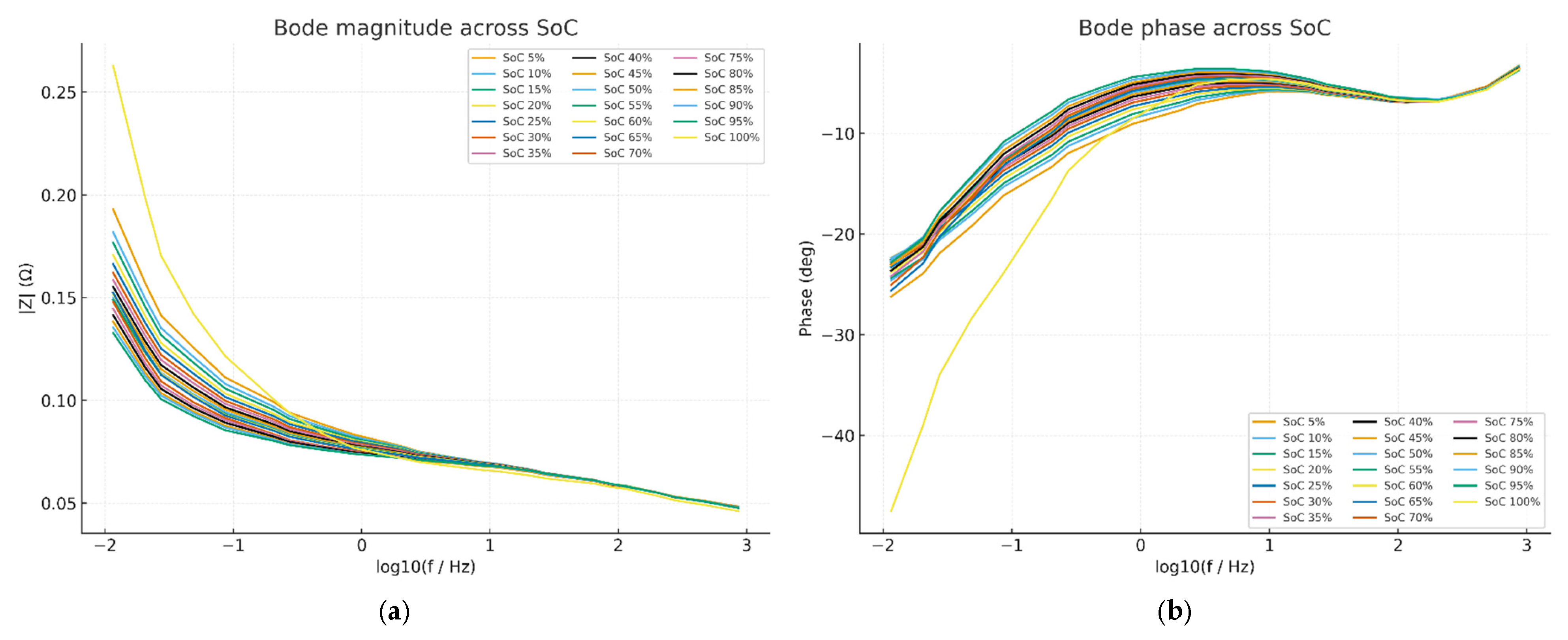
The impedance spectrum data, obtained using Electrochemical Impedance Spectroscopy (EIS), characterizes the battery’s internal resistance and dynamic behavior. This behavior is presented as Nyquist plots and Bode plots, as shown in Figure 2 and Figure 3. As the battery cell’s state of charge changes, its internal resistance varies, affecting impedance values. Generally, impedance is higher at lower SOC due to slower reaction kinetics and limited ion mobility [20]. The SOC variations are reflected clearly in the medium-frequency region (charge-transfer processes) and the low-frequency region (diffusion-controlled processes). Typically, the semicircle diameter (charge-transfer resistance) in the Nyquist plot increases notably at lower SOC. It affects electrode kinetics, thereby shifting the impedance spectrum. Changes in SOC alter electrode potential, affecting both the charge-transfer resistance and double-layer capacitance. Generally, the impedance spectrum directly reflects the battery SOC through changes in internal resistance and electrochemical kinetics—a potential method of accurate SOC estimation [20,21].

Figure 2. Aggregated Nyquist plots across SOCs from cell’s EIS data in [19].

Figure 3. Aggregated (a) Bode magnitude and (b) Bode phase plots across SOCs from cell’s EIS data in [19].

In the Nyquist $\left(Re\right\{Z\} vs -Im\{Z\left\}\right)$ in Figure 2, the high-frequency (HF) intercept (ohmic resistance) shifts modestly with SoC, usually lowest near mid-SoC and higher at very low/high SoC. The medium-frequency (MF) semicircle (charge-transfer) changes in radius and center with SoC; lower SoC typically shows a larger arc (higher polarization), while higher SoC compresses the arc.

The low-frequency (LF) tail (diffusion) slope varies with SoC, reflecting changes in mass transport; this tail, plus the arc shape, produces a monotonic morphological trend across SoC.

Bode $\left|Z\right|$ and phase (vs log10 f) curves in Figure 3a,b separate most clearly from mid- to low-frequencies; high SoC sits lower (lower impedance), low SoC sits higher. Phase becomes less negative as SoC increases; the spread between SoCs is largest around the MF–LF band. These frequency bands are where the SoC sensitivity is strongest and thus where most of the predictive signal resides.

2.4. Machine Learning Algorithms

We implemented all models in Python (NumPy, pandas, Matplotlib, scikit-learn; XGBoost for XGBRegressor). The dataset features were frequency (Hz), R (ohm), X (ohm), V (V), T (°C), and range (Ohm), with SoC as the target; data were split 80/20 (train/test) with random state = 42. No imputation was required; we used raw features, consistent with the main code. Hyperparameters followed canonical defaults with light adjustments, as summarized in Table 1. Models were trained on the 80% split and evaluated on the 20% hold-out using RMSE and R², with parity and error distribution plots reported in the Section 3.

We implemented and tuned five different ML algorithms to learn the mapping from EIS data to SoC. Each algorithm has different assumptions and characteristics, which we briefly describe below, along with reasons it might be suitable for this task.

2.4.1. Random Forest (RF)

Random Forest is an ensemble learning method that constructs a large number of decision trees using bootstrapped samples of the data and random feature subsets at each split, and averages their predictions [22,23]. Conceptually, each decision tree partitions the feature space—in this case, the space of impedance spectra—according to thresholding rules, and the ensemble average tends to reduce overfitting and improve robustness [24,25]. RF can capture highly nonlinear relationships and feature interactions without requiring feature scaling or explicit domain knowledge. This makes it particularly suitable for SoC estimation from EIS, as the relationship between impedance at different frequencies and SoC is complex. The ensemble nature of RF also tends to make it robust to noise and outliers. A possible downside is that if the number of features is large relative to the number of training samples, trees might still overfit specific patterns; however, the random feature selection in RF helps mitigate this. In this study, Random Forest performed exceptionally well, likely because it could model the intricate footprints of the impedance spectrum at each SoC, as shown in the Section 3. Prior work has identified Random Forest regression as one of the most effective tools for data-driven SoC estimation [19].

2.4.2. Gradient Boosting (GB)

Gradient Boosting machines build an ensemble of decision trees sequentially, where each new tree is trained to correct the errors of the previous ensemble [26]. The model starts with a simple predictor and adds trees that improve performance by focusing on examples that were previously misclassified [26]. This yields a strong predictive model often with high accuracy. For SoC estimation, Gradient Boosting is attractive because it directly optimizes a loss (e.g., MSE) and can model nonlinear relationships with high fidelity [26,27,28]. This work used a Gradient Boosting regressor (e.g., the Scikit-Learn implementation), which typically requires specifying parameters such as the number of trees, tree depth, and learning rate. If tuned properly, GB can achieve performance comparable to Random Forest. One reason it is suitable for EIS data is its ability to handle feature interactions and nonlinearity, similar to RF, but with a different bias-variance trade-off (boosting can sometimes achieve lower bias at the cost of being more prone to overfitting if not regularized). In practice, our Gradient Boosting model achieved very high accuracy (nearly perfect R²), indicating that it successfully learned the EIS–SoC mapping. The careful use of regularization is important to ensure the model generalizes rather than memorizes the training data.

2.4.3. XGBoost (Extreme Gradient Boosting)

This is a popular, optimized implementation of Gradient Boosting that includes additional regularization and efficiency improvements [29]. Conceptually, it is similar to the GB described above, building trees sequentially to minimize the error [30]. XGBoost often yields top performance in structured data competitions due to features such as tree pruning, a regularized objective, and fast handling of missing data. For our SoC task, this work used XGBoost as another boosting variant to compare with the standard GB. We expected XGBoost to perform on par with, or better than, generic Gradient Boosting, thanks to its regularization, which can prevent overfitting even with many trees. Indeed, XGBoost achieved almost identical performance (R²~1.00) in our experiments, indicating that it effectively captured the complex mapping from impedance features to SoC while maintaining generalization. The advantage of XGBoost for SoC estimation is its balance of flexibility and regularization—it can fit very complex functions while also including parameters (such as L1/L2 penalties and tree complexity limits) to prevent the model from becoming overly complex for the data.

2.4.4. AdaBoost

Adaptive Boosting is another boosting technique that differs from Gradient Boosting in how it builds the ensemble [26,31]. In AdaBoost, each new weak learner (often a shallow decision tree, e.g., a decision stump) is trained on the training set with adjusted sample weights: it pays more attention to data points that previous learners predicted wrong [31,32,33]. The final prediction is a weighted sum of the weak learners. For SoC estimation, AdaBoost can be used to assess whether a simpler boosting method with very weak learners can capture the EIS-to-SoC relationship [33]. Its potential advantage is simplicity and interpretability (when using very simple base models), but it may require many weak learners to fit a complex function. Since EIS data patterns might be quite nonlinear, it was anticipated that AdaBoost might underperform Gradient Boosting or RF because using very shallow trees can make it hard to capture all the nuances of the impedance spectra. Our results showed that AdaBoost achieved high accuracy (R² ≈ 0.99), but not as well as the other tree ensembles, and it had a slightly higher MSE. This suggests that AdaBoost learned the general trend but perhaps struggled with subtle variations, consistent with the idea that its weaker base models had limited capacity. AdaBoost may also be somewhat sensitive to outliers or noise (as it focuses on “hard” samples), which could be a factor if any impedance measurements were noisy.

2.4.5. Extra Trees (Extremely Randomized Trees)

The Extra Trees algorithm is another ensemble of decision trees similar to Random Forest. However, it has one key difference: when splitting nodes, it selects split thresholds thoroughly at random for each candidate feature (instead of choosing the optimal split) [34,35,36]. In essence, Extra Trees injects more randomness into tree building than RF, which can further reduce variance at the cost of a slight increase in bias [36]. Extra Trees typically uses the full dataset (no bootstrap sampling by default) and random splits [34,35]. For SoC estimation, Extra Trees has similar benefits to RF: the ability to model complex interactions and nonlinear effects. The extra randomness can sometimes make the ensemble more robust to overfitting and faster to train (since it does not search for the best split). In our experiments, the Extra Trees model was among the top performers, achieving essentially perfect prediction of the test data (slightly better MSE than RF). This indicates that the added randomness did not hinder the development of an accurate model and perhaps even helped with generalization. Extra Trees would be suitable in scenarios where a strong ensemble model is needed quickly or to reduce variance; given the consistency of EIS patterns across SoCs, the model likely benefits from the diversity of trees to avoid locking onto noise in the training data.

3. Results

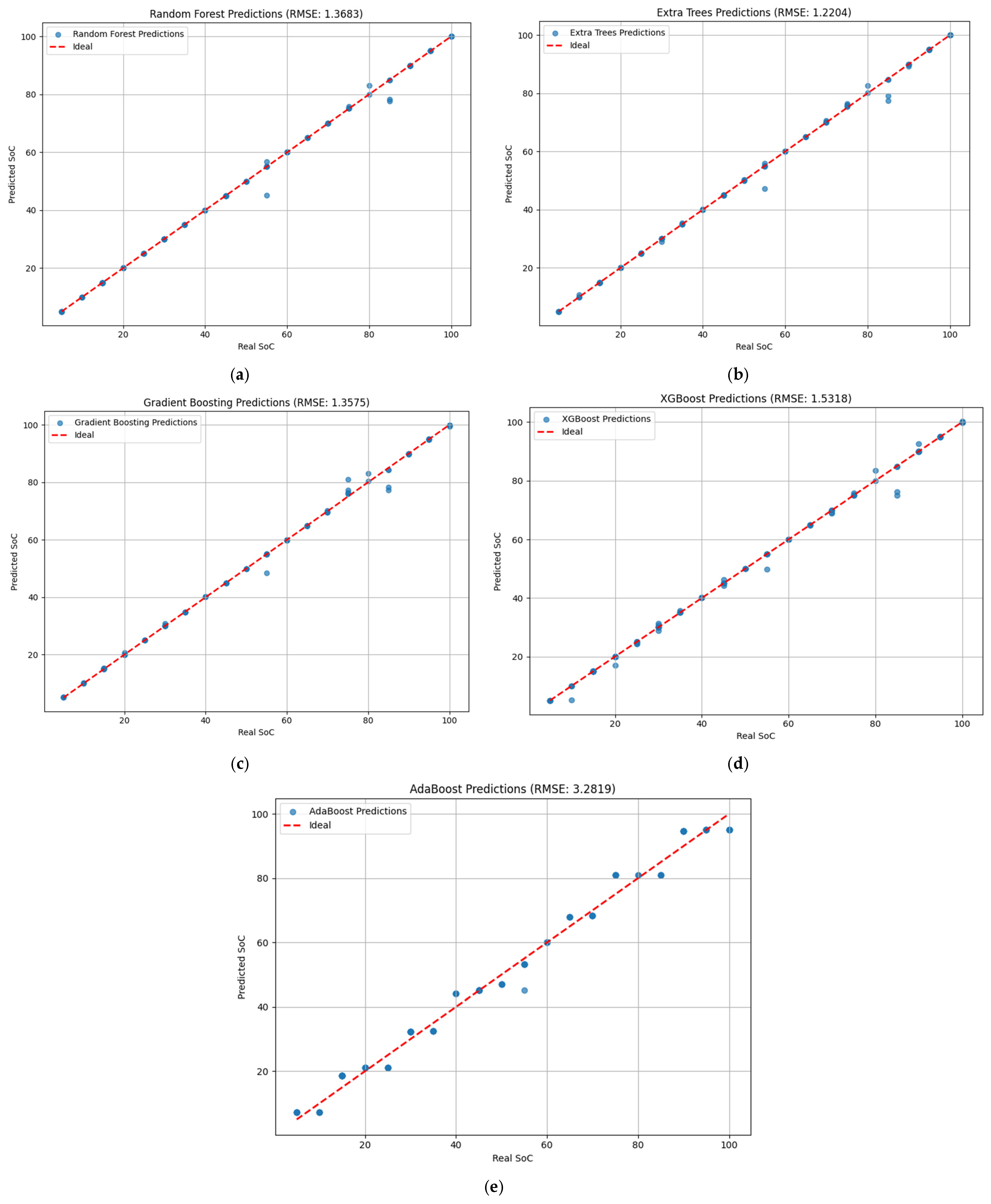
After training each model on the EIS dataset, the performance was evaluated on the held-out test data using the Mean Squared Error (MSE) and R² metrics. Table 3 summarizes the quantitative performance of all five models. A higher R² and lower MSE indicate better accuracy. It is also corroborated by the following plots in Figure 4a–e.

Table 3. Summary of the quantitative performance of all five models.

Model	Test MSE	Test RMSE	R2
Random Forest	1.90	1.378	0.9977
Extra Trees	1.76	1.327	0.9979
Gradient Boosting	2.35	1.533	0.9972
XGBoost	2.42	1.556	0.9971
AdaBoost	9.38	3.063	0.9887

Figure 4. Predicted vs. actual SoC performance results for all five models. Each subplot corresponds to one model. The red dashed diagonal line in each plot represents the ideal prediction (perfect accuracy). (a) Random Forest (RF); (b) Extra Tree; (c) Gradient Boosting; (d) Extreme Gradient Boosting; (e) Adaptive Boosting. Models whose points lie close to this line for all SoC values are highly accurate, whereas significant deviations from the line indicate prediction errors.

4. Discussion

4.1. Quantitative Performance

Table 3 presents the test set metrics for the five models. All tree ensemble methods achieved very low SoC predicted errors and almost a perfect fit (R² ≈ 1.00), with Extra Trees giving the lowest MSE (1.76; RMSE = 1.33), followed closely by Random Forest (MSE = 1.90; RMSE = 1.38), Gradient Boosting (MSE = 2.35; RMSE = 1.53), and XGBoost (MSE = 2.42; RMSE = 1.56). AdaBoost performed worse than the other ensembles but still delivered strong accuracy (MSE = 9.38; RMSE = 3.06). The small spread among the top four models indicates that the EIS features contain a strong and learnable mapping to SoC that modern tree ensembles can capture reliably.

4.2. Visual Assessment from Plots in Figure 4

The predicted vs. actual SoC plots further corroborate the quantitative performance metrics. Figure 4a Random Forest and Figure 4b Extra Trees: Points lie tightly on the true SoC line across the full SoC range, indicating negligible bias and low variance. Occasional minor deviations occur at mid–high SoC (75–85%), but they are within ±2–3% SoC, consistent with the 1.3–1.4 RMSE.

Figure 4c Gradient Boosting and Figure 4d XGBoost: Trends are similarly linear with slightly larger scatter than RF/Extra Trees, again most visible near the upper-SoC region. This is reflected in the modestly higher RMSE (1.5–1.6). The behavior is typical of boosted trees with shallow base learners that trade a bit of variance for bias control.

Figure 4e AdaBoost: Points still follow the ideal line but with noticeably wider dispersion, particularly in the mid-range (40–70% SoC) and near the upper end. This increased spread explains the higher RMSE (3.06). Given AdaBoost’s reliance on weak base learners (often decision stumps or very shallow trees), its capacity to model the multi-frequency, nonlinear EIS-to-SoC mapping is comparatively limited.

4.3. Prediction Error Analysis Across Ensemble Models from Figure 5

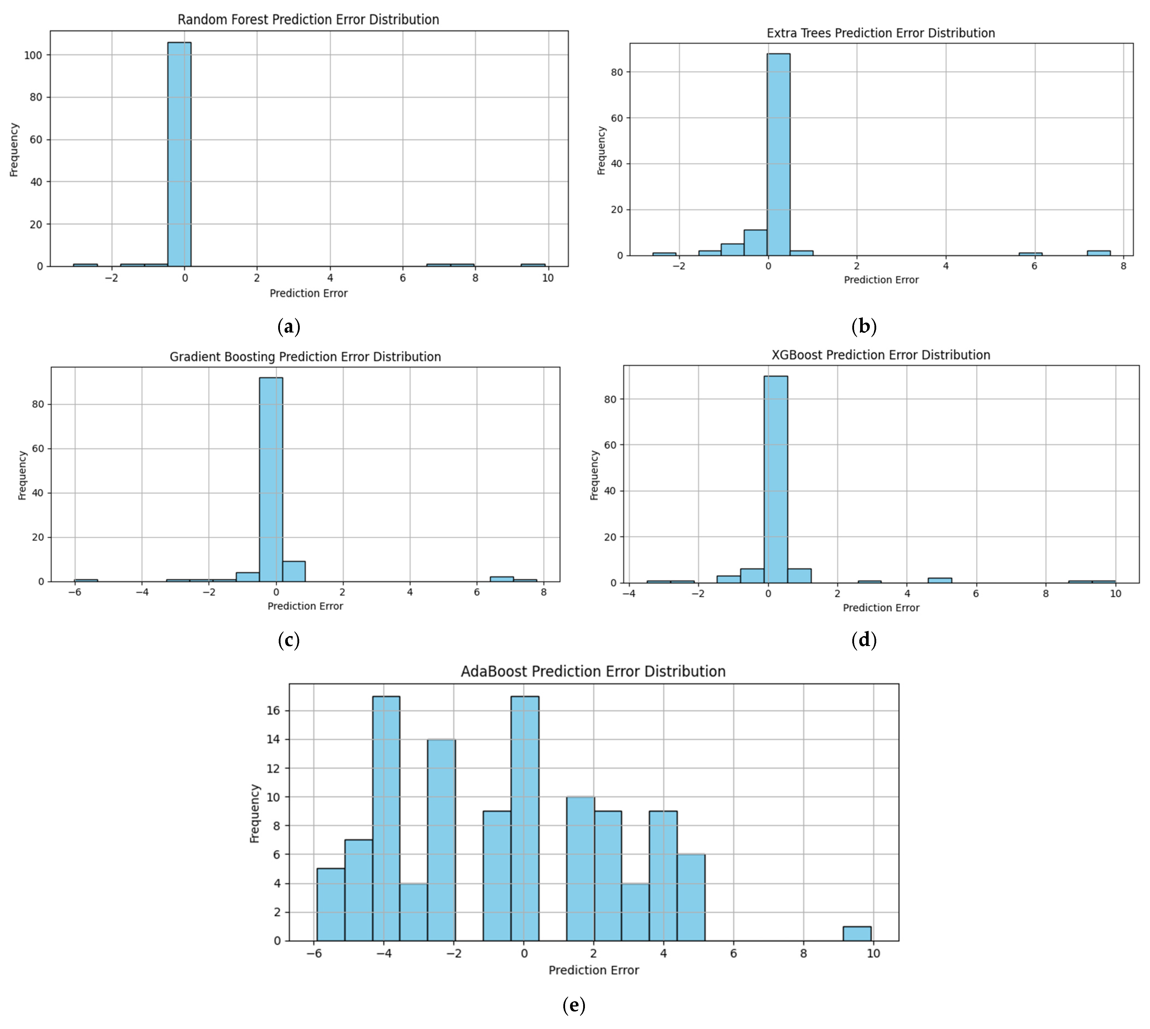
Figure 5. Error plots of the five machine learning algorithms representing the difference between the actual and predicted state of charge (SoC) values. (a) Random Forest (RF); (b) Extra Tree; (c) Gradient Boosting; (d) Extreme Gradient Boosting; (e) Adaptive Boosting.

Figure 5 presents the prediction error distributions for five tree-based ensemble models: Figure 5a for Random Forest (RF), Figure 5b for Extra Tree, Figure 5c for Gradient Boosting, Figure 5d for Extreme Gradient Boosting, and Figure 5e for Adaptive Boosting. The prediction error is defined as follows:

$$Error=Predicted SoC-True SoC$$

(8)

General observation from the error plots across models: The absolute error concentrates in the mid–high SoC region—most visibly around 40–70% SoC and, to a lesser extent, around 75–85%. This is consistent with EIS physics: in this band, the charge-transfer arc and LF diffusion slope change more slowly with SoC, so the spectra are less separable, the SoC signal-to-noise ratio drops, and predictions become harder. Minor contributors include label discretization, temperature, and any imbalance in sample counts across SoC. The effect is most pronounced for AdaBoost (shallower base learners), while Extra Trees/Random Forest remain tighter by capturing deeper cross-frequency interactions.

Random Forest: The Random Forest model shows the most concentrated error peak at zero, with negligible bias and very low variance. Few isolated extreme positive errors (+8–10%) exist, but their frequency is minimal. The tight distribution aligns with its strong RMSE (1.38).

Extra Trees: Extra Trees produce the most compact error spread among all models, explaining its best RMSE (1.33). Its higher randomness in split selection likely reduces overfitting and variance, making its predictions both accurate and stable.

Gradient Boosting: The histogram is strongly peaked at zero, indicating high prediction accuracy and low bias. A few moderate outliers (−6% and +8%) appear, suggesting occasional misestimation in challenging SoC regions, possibly where EIS features change subtly. The narrow spread matches its low RMSE (~1.53).

XGBoost: Similarly to Gradient Boosting, XGBoost’s errors are centered at zero with a slightly longer right tail, indicating rare overpredictions up to +10%. Its performance (RMSE ~1.56) reflects high accuracy, with most deviations being small and infrequent.

AdaBoost: In contrast, AdaBoost’s error distribution is much wider, spanning approximately −6% to +10% SoC. The central peak near zero is less pronounced, and there is a higher frequency of moderate-to-large deviations. This broader spread corresponds to its weaker performance (RMSE~3.06, R² = 0.99), suggesting that AdaBoost’s weaker base learners are less capable of capturing the complex nonlinear relationships in the EIS–SoC mapping.

4.4. Implications

Bias and Accuracy: All models exhibit error distributions tightly centered around zero, indicating minimal bias and strong predictive accuracy.

Variance: Extra Trees and Random Forest have the lowest error variance, while boosting methods show slightly greater spread.

Outliers: Boosting methods (particularly AdaBoost) are more prone to outliers, which can disproportionately increase RMSE.

Model Suitability: For EIS-based SoC estimation, Extra Trees and Random Forest are best suited when stability and minimal variance are critical. Gradient Boosting and XGBoost provide competitive accuracy with slight trade-offs in variance. AdaBoost underperforms for this application due to its larger residual spread.

5. Conclusions

This study evaluated multiple tree-based ensemble algorithms (Random Forest, Extra Trees, Gradient Boosting, XGBoost, AdaBoost) for estimating lithium-ion SoC from EIS spectra, achieving ~1.3–1.6% SoC RMSE for the top performers under leakage-aware evaluation. Compared with prior EIS-ML SoC work, our contribution is distinguished by use of a public, DOI-backed dataset, spectrum-grouped validation, multi-model benchmarking, and richer error diagnostics, supporting reproducibility and credible generalization.

Real-world application and BMS integration: These models are well-suited for battery management systems (BMSs) as a complementary “snapshot” estimator: an impedance sweep (or a compressed subset of frequencies) can be taken opportunistically—e.g., during parked/idle periods, scheduled maintenance, or charge pauses—to refresh SoC estimates and calibrate model-based observers. In electric vehicles and stationary energy storage, the ensemble models’ modest computational requirements enable edge deployment (CPU-only), while their feature importances provide interpretable checks for safety and diagnostics. In practice, EIS-ML can serve as a periodic calibrator for OCV/Kalman pipelines, reducing drift and improving accuracy without requiring full charge/discharge cycles.

Future directions: We see three immediate avenues: (i) hybrid estimators that fuse EIS-ML with Kalman/EKF/UKF or OCV maps for continuous operation, (ii) real-time data integration, including temperature/voltage context and adaptive frequency selection to shorten sweeps, and (iii) transfer learning/domain adaptation to extend across chemistries, suppliers, and aging states, with uncertainty quantification to gate control actions.

Limitations: This study lacks independent external validation from a different lab or chemistry; while grouped and cell-level validations reduce optimism, external testing remains to be conducted in future work. Future studies can also explore hybrid models, expanded feature engineering, and online/embedded implementations to improve further accuracy in challenging SoC regions and across battery chemistries. This study is based on the EIS bandwidth (1 mHz–1 kHz) from a public datasheet, which is sufficient for SoC-informative charge-transfer and diffusion features. Future work can extend measurements to ≥10 kHz to assess any additional possible benefits of higher-frequency content for SoC estimation and model robustness.

References

1. Kunatsa, T.; Myburgh, H.C.; De Freitas, A. A Review on State-of-Charge Estimation Methods, Energy Storage Technologies and State-of-the-Art Simulators: Recent Developments and Challenges. World Electr. Veh. J. 2024, 15, 381. [Google Scholar] [CrossRef]
2. Guo, D.; Guo, P.; Sun, L. Estimation of Battery State of Charge Based on Electrochemical Impedance Spectroscopy and Machine Learning. J. Phys. Conf. Ser. 2023, 2661, 012025. [Google Scholar] [CrossRef]
3. Soyoye, B.D.; Bhattacharya, I.; Anthony Dhason, M.V.; Banik, T. State of Charge and State of Health Estimation in Electric Vehicles: Challenges, Approaches and Future Directions. Batteries 2025, 11, 32. [Google Scholar] [CrossRef]
4. Hussein, H.M.; Esoofally, M.; Donekal, A.; Rafin, S.M.S.H.; Mohammed, O. Comparative Study-Based Data-Driven Models for Lithium-Ion Battery State-of-Charge Estimation. Batteries 2024, 10, 89. [Google Scholar] [CrossRef]
5. Shingote, S.; Shejwalkar, A.; Swain, S. Comparative Analysis for State-of-Charge Estimation of Lithium-Ion Batteries using Non-Linear Kalman Filters. In Proceedings of the 2023 IEEE 3rd International Conference on Sustainable Energy and Future Electric Transportation (SEFET), Bhubaneswar, India, 9–12 August 2023. [Google Scholar] [CrossRef]
6. Buchicchio, E.; De Angelis, A.; Santoni, F.; Carbone, P. Lithium-Ion Batteries state of charge estimation based on electrochemical impedance spectroscopy and convolutional neural network. In Proceedings of the 25th IMEKO TC4 International Symposium and the 23rd International Workshop on ADC and DAC Modelling and Testing, Brescia, Italy, 12–14 September 2022. [Google Scholar]
7. Guo, K.; Zhu, Y.; Zhong, Y.; Wu, K.; Yang, F. An Informer-LSTM Network for State-of-Charge Estimation of Lithium-Ion Batteries. In Proceedings of the 2023 Global Reliability and Prognostics and Health Management Conference (PHM-Hangzhou), Hangzhou, China, 12–15 October 2023. [Google Scholar] [CrossRef]
8. Lazanas, A.C.; Prodromidis, M.I. Electrochemical Impedance Spectroscopy—A Tutorial. ACS Meas. Sci. Au 2023, 3, 162–193. [Google Scholar] [CrossRef]
9. Peng, Y.; Hu, H.; Geng, A.; Chen, Y.; Zhao, Z. An Electrochemical Impedance Spectroscopy-Based Model for Lithium-Ion Batteries with Solid Phase Diffusion Process. In Proceedings of the PEAS 2023—2023 IEEE 2nd International Power Electronics and Application Symposium, Guangzhou, China, 10–13 October 2023; pp. 887–891. [Google Scholar] [CrossRef]
10. Nunes, H.; Martinho, J.; Fermeiro, J.; Pombo, J.; Mariano, S.; do Rosário Calado, M. Impedance Analysis and Parameter Estimation of Lithium-Ion Batteries Using the EIS Technique. IEEE Trans. Ind. Appl. 2024, 60, 5048–5060. [Google Scholar] [CrossRef]
11. Kanoun, O.; Kallel, A.Y.; Nouri, H.; Atitallah, B.B.; Haddad, D.; Hu, Z.; Talbi, M.; Al-Hamry, A.; Munja, R.; Wendler, F.; et al. Impedance Spectroscopy: Applications, Advances and Future Trends. IEEE Instrum. Meas. Mag. 2022, 25, 11–21. [Google Scholar] [CrossRef]
12. Barsoukov, E.; Macdonald, J.R. (Eds.) Impedance Spectroscopy; Wiley: Hoboken, NJ, USA, 2018. [Google Scholar] [CrossRef]
13. Li, D.; Yang, D.; Li, L.; Wang, L.; Wang, K. Electrochemical Impedance Spectroscopy Based on the State of Health Estimation for Lithium-Ion Batteries. Energies 2022, 15, 6665. [Google Scholar] [CrossRef]
14. Ranjith Kumar, R.; Bharatiraja, C.; Udhayakumar, K.; Devakirubakaran, S.; Sekar, K.S.; Mihet-Popa, L. Advances in Batteries, Battery Modeling, Battery Management System, Battery Thermal Management, SOC, SOH, and Charge/Discharge Characteristics in EV Applications. IEEE Access 2023, 11, 105761–105809. [Google Scholar] [CrossRef]
15. Wang, C.; Yang, M.; Wang, X.; Xiong, Z.; Qian, F.; Deng, C.; Yu, C.; Zhang, Z.; Guo, X. A review of battery SOC estimation based on equivalent circuit models. J. Energy Storage 2025, 110, 115346. [Google Scholar] [CrossRef]
16. Baccouche, I.; Jemmali, S.; Manai, B.; Omar, N.; Essoukri Ben Amara, N. Improved OCV model of a Li-ion NMC battery for online SOC estimation using the extended Kalman filter. Energies 2017, 10, 764. [Google Scholar] [CrossRef]
17. Monirul, I.M.; Qiu, L.; Ruby, R.; Ullah, I.; Sharafian, A. Accurate SOC estimation in power lithium-ion batteries using adaptive extended Kalman filter with a high-order electrical equivalent circuit model. Measurement 2025, 249, 117081. [Google Scholar] [CrossRef]
18. Bourelly, C.; Vitelli, M.; Milano, F.; Molinara, M.; Fontanella, F.; Ferrigno, L. EIS-Based SoC Estimation: A Novel Measurement Method for Optimizing Accuracy and Measurement Time. IEEE Access 2023, 11, 91472–91484. [Google Scholar] [CrossRef]
19. Mustafa, H.; Bourelly, C.; Vitelli, M.; Milano, F.; Molinara, M.; Ferrigno, L. SoC estimation on Li-ion batteries: A new EIS-based dataset for data-driven applications. Data Brief 2024, 57, 110947. [Google Scholar] [CrossRef]
20. Pisani Orta, M.A.; García Elvira, D.; Valderrama Blaví, H. Review of State-of-Charge Estimation Methods for Electric Vehicle Applications. World Electr. Veh. J. 2025, 16, 87. [Google Scholar] [CrossRef]
21. Hosen, M.S.; Gopalakrishnan, R.; Kalogiannis, T.; Jaguemont, J.; Van Mierlo, J.; Berecibar, M. Impact of Relaxation Time on Electrochemical Impedance Spectroscopy Characterization of the Most Common Lithium Battery Technologies—Experimental Study and Chemistry-Neutral Modeling. World Electr. Veh. J. 2021, 12, 77. [Google Scholar] [CrossRef]
22. Breiman, L. Random Forests. Mach. Learn. 2001, 45, 5–32. [Google Scholar] [CrossRef]
23. Ho, T.K. Random decision forests. In Proceedings of the 3rd International Conference on Document Analysis and Recognition, Washington, DC, USA, 14–15 August 1995; pp. 278–282. [Google Scholar] [CrossRef]
24. Borup, D.; Christensen, B.J.; Mühlbach, N.S.; Nielsen, M.S. Targeting predictors in random forest regression. Int. J. Forecast. 2023, 39, 841–868. [Google Scholar] [CrossRef]
25. Baalousha, H.M. Machine learning approaches for groundwater vulnerability assessment in arid environments: Enhancing DRASTIC with ANN and Random Forest. Groundw. Sustain. Dev. 2025, 30, 101496. [Google Scholar] [CrossRef]
26. Hastie, T.; Tibshirani, R.; Friedman, J. The Elements of Statistical Learning; Springer: New York, NY, USA, 2009. [Google Scholar] [CrossRef]
27. Khawaja, Y.; Shankar, N.; Qiqieh, I.; Alzubi, J.; Alzubi, O.; Nallakaruppan, M.K.; Padmanaban, S. Battery management solutions for li-ion batteries based on artificial intelligence. Ain Shams Eng. J. 2023, 14, 102213. [Google Scholar] [CrossRef]
28. Oyucu, S.; Ersöz, B.; Sağıroğlu, Ş.; Aksöz, A.; Biçer, E. Optimizing Lithium-Ion Battery Performance: Integrating Machine Learning and Explainable AI for Enhanced Energy Management. Sustainability 2024, 16, 4755. [Google Scholar] [CrossRef]
29. Chen, T.; Guestrin, C. XGBoost: A Scalable Tree Boosting System. In Proceedings of the 22nd ACM SIGKDD International Conference on Knowledge Discovery and Data Mining, San Francisco, CA, USA, 13–17 August 2016; ACM: New York, NY, USA, 2016; pp. 785–794. [Google Scholar] [CrossRef]
30. Baalousha, H.M. Machine Learning-Driven Calibration of MODFLOW Models: Comparing Random Forest and XGBoost Approaches. Geosciences 2025, 15, 303. [Google Scholar] [CrossRef]
31. Ding, Y.; Zhu, H.; Chen, R.; Li, R. An Efficient AdaBoost Algorithm with the Multiple Thresholds Classification. Appl. Sci. 2022, 12, 5872. [Google Scholar] [CrossRef]
32. Taherkhani, A.; Cosma, G.; McGinnity, T.M. AdaBoost-CNN: An adaptive boosting algorithm for convolutional neural networks to classify multi-class imbalanced datasets using transfer learning. Neurocomputing 2020, 404, 351–366. [Google Scholar] [CrossRef]
33. Liu, B.; Liu, C.; Xiao, Y.; Liu, L.; Li, W.; Chen, X. AdaBoost-based transfer learning method for positive and unlabelled learning problem. Knowl.-Based Syst. 2022, 241, 108162. [Google Scholar] [CrossRef]
34. Berrouachedi, A.; Jaziri, R.; Bernard, G. Deep Extremely Randomized Trees; Springer: Berlin/Heidelberg, Germany, 2019; pp. 717–729. [Google Scholar] [CrossRef]
35. Geurts, P.; Ernst, D.; Wehenkel, L. Extremely randomized trees. Mach. Learn. 2006, 63, 3–42. [Google Scholar] [CrossRef]
36. Pagliaro, A. Forecasting Significant Stock Market Price Changes Using Machine Learning: Extra Trees Classifier Leads. Electronics 2023, 12, 4551. [Google Scholar] [CrossRef]
Disclaimer/Publisher’s Note: The statements, opinions and data contained in all publications are solely those of the individual author(s) and contributor(s) and not of MDPI and/or the editor(s). MDPI and/or the editor(s) disclaim responsibility for any injury to people or property resulting from any ideas, methods, instructions or products referred to in the content.
Article Metrics
Citations
Article Access Statistics
Multiple requests from the same IP address are counted as one view.