Framework and Layer-Wise Word-Line Activation Method Design for CIM

Abstract

Convolutional Neural Networks (CNNs) have excellent performance in various fields, such as machine learning, computer vision, and image recognition. With the development of CNNs, huge quantities of data in computing and transmission have placed significant pressure on circuit and architecture design, and RRAM-based computing-in-memory (CIM) is one of the promising solutions to alleviate this problem. However, because of the current deviation phenomenon and the resistance on/off ratio (R ratio) issue in RRAM, there is a trade-off problem between computational accuracy and computational efficiency for CIM. In this paper, we propose a layer-wise activated word-line (AWL) strategy to configure the appropriate number of AWLs for each layer. Based on the observed risk factors, we design a risk index to AWL mapping methodology. Meanwhile, based on the proposed quantization and current deviation error calculation methods, we design a CIM simulation framework to simulate the accuracy of CNNs in the inference stage. We evaluate our methodology on Cifar-10, VGG-8, and ResNet-18. The proposed methodology improves computational efficiency with only slight accuracy loss. In comparison with a fixed-AWL configuration, our methodology has better accuracy with a small resistance on/off ratio. For higher resistance on/off ratios, our methodology gets a significant improvement in computational efficiency in comparison with the baseline. On the exploration of different R ratios, experimental results show that our layer-wise AWL configuration methodology has a more flexible planning space and better computational efficiency.

1. Introduction

Overview

Convolutional Neural Networks (CNNs) [1] have excellent performance in many fields, such as machine learning, computer vision, and image recognition [2]. Their brilliant performance depends on massive amounts of calculations. In recent years, the CNN architecture has become much deeper and more complex than before; large amounts of memory access often represent a bottleneck that affects the performance and energy consumption of hardware accelerators. Therefore, reducing the access distance between the chip’s external memory and the computing unit or integrating computing power into the memory is a research trend in the architectural design of CNN hardware accelerators [1,2,3]. Among them, methods to reduce the distance between the chip’s external memory and the computing unit include embedded memory (embedded DRAM) or stacking the memory on the computing unit in a three-dimensional manner.

In order to reduce the power consumption and delay caused by data relocation during CNN calculations, in addition to placing the on-chip memory close to the computing unit, another way is to use the computing-in-memory architecture. MAC operations can be integrated into the bit cells of SRAM or non-volatile resistive memory (RRAM). Research results [4] show that the computing-in-memory architecture can further improve performance and reduce power consumption. Therefore, computing-in-memory techniques are expected to be a future direction to reduce the amount of external data migration. Some previous works [1,5] have used CIM techniques to successfully reduce large amounts of external data migration during CNN computations.

CIM is a technique to reduce data migration in CNN computation [3]. Its computational architecture and operation method are illustrated in Figure 1. An input feature map (IFP) is input into the CIM array from word lines (WLs) in the form of voltage. Weights are stored in memory cells in the form of conductance. The currents produced by memory cells accumulate along the bit-line (BL) and then through the ADC and shifter to be converted into computational results.

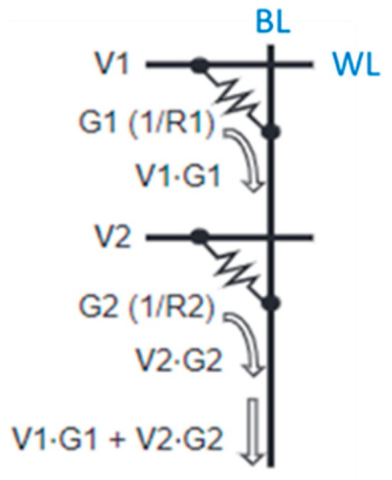
Figure 1. CIM computing architecture.

Computational memory circuits can be roughly divided into two categories: volatile computing-in-memory circuits and non-volatile computing-in-memory circuits. Volatile computing-in-memory circuits are mainly implemented with SRAM; non-volatile computing-in-memory circuits are mainly implemented with RRAM. RRAM has the advantages of short reading latency, low area cost, and near to zero leakage power [6]. Therefore, it is a good choice for computational memory in the CIM architecture [7].

The RRAM crossbar array inherently supports highly parallel in-memory dot product operations. However, the current flowing through the bit line which corresponds to the dot product output can result in a wrong value because of the RRAM cell’s high-resistance state. Ideally, the current generated by the high-resistance RRAM cell should be zero, but in reality, a high-resistance RRAM cell will still generate a weak current, which will reduce the computational accuracy [8].

This error-prone nature of RRAM crossbars imposes a restriction on their parallel execution. Ideally, we would activate all word lines at the same time to complete many computations, but in actuality, more AWLs means more errors are accumulated. Therefore, many studies [9,10,11] limit the number of AWLs activated at a time to avoid error accumulation, hence having a negative impact on the computational efficiency of CIM architectures. Although Ref. [3] proposes that the maximum number of AWLs for each neural layer can be different, their methodology requires an exhaustive search starting from the baseline and therefore is not practical for large neural networks.

In this paper, we propose a layer-wise AWL strategy to configure the appropriate number of AWLs for each neural layer. Our AWL configuration also takes into account the effect of the resistance on/off ratio (R ratio); based on the observed risk factors, we design a risk index to AWL mapping methodology. Meanwhile, based on the proposed quantization and current deviation error calculation methods, we design a CIM simulation framework to simulate the accuracy of CNNs in the inference stage.

In summary, our work makes the following contributions:

• We propose a simple but efficient risk factor and risk index mapping methodology for layer-wise AWL configuration. The proposed methodology improves computational efficiency with only slight accuracy loss.
• We can easily fine-tune risk factors and index mapping to fit different scales of neural networks and reduce the AWL configuration loading of large AI models.
• In comparison with the fixed-AWL configuration, our methodology has better computational accuracy with small resistance on/off ratios.
• For higher resistance on/off ratios, our methodology shows a significant improvement in computational efficiency in comparison with the baseline.

The rest of this paper is organized as follows: In Section 2, we describe the background and motivation of the layer-wise AWL configuration and the effect of current deviation and resistance on/off ratio on computational accuracy and computational efficiency. Section 3 describes our inference accuracy predictor and layer-wise AWL configuration strategy, including risk index-to-AWL mapping, and quantization and current deviation error calculation methods. In Section 4, we show the results of our methodology on Cifar-10, VGG-8, and ResNet-18 and analyze and discuss the effect of different R ratios. Finally, we draw conclusions in Section 5.

2. Background and Motivation

2.1. Background

2.1.1. Current Deviation

Some features of RRAM may influence the CIM array’s computation result, and the most important one is current deviation. RRAM consists two metal layers and one transition metal oxide layer, where the transition metal oxide layer is between the two metal layers. By applying an external bias to RRAM, an oxidation channel connecting the two metal layers forms in the transition metal oxide layer, a state known as the low-resistance state (LRS). Applying an external bias to cut off the oxidation channel in the transition metal oxide layer results in a high-resistance state (HRS). By applying different biases, RRAM transits between the low-resistance state and the high-resistance state. Since the resistance value is affected by the external bias which in turn affects the formation or interruption of the oxidation channel, the generated resistance value is not a constant value.

In RRAM CIM calculation, a current I_LRS is generated through a low-resistance RRAM cell, and a current I_HRS is generated through a high-resistance RRAM cell. Then the current accumulated by cells of the same bit line is converted through an analog-to-digital converter and a shifter to obtain the final calculation result. Ideally, the current generated by the high-resistance RRAM cell should be zero (I_HRS = 0), which means that only I_LRS accumulates and participates in the subsequent conversion process. However, in reality, a high-resistance RRAM cell still generates a weak current (I_HRS ≠ 0), and the accumulation of multiple I_HRS exceeds the tolerance range of the analog-to-digital converter, causing errors. For example, in Figure 2, there are one HRS cell and three LRS memory cells on the leftmost bit line. The ideal situation is the accumulation of current $I_{ideal}$ = 3 × $I_{LRS}$, but the real situation shows $I_{total}$ = $I_{HRS}$ + 3 × $I_{LRS}$. The extra $I_{HRS}$ may cause an error in the result.

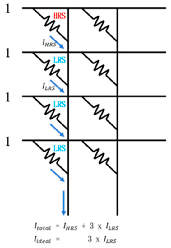
Figure 2. Example of current deviation.

2.1.2. Resistance on/off Ratio (R Ratio)

The resistance on/off ratio is the ratio of the high-resistance value to the low-resistance value (R_HRS/R_LRS = R OFF/R ON). As shown in the formula in Figure 3, we assume that the resistance on/off ratio is 10 and the voltage is 1, that is, R_HRS:R_LRS = 10:1. Through the formula I = V/R, we get I_HRS:I_LRS = 1:10, and finally, we get 10 × I_HRS = I_LRS.

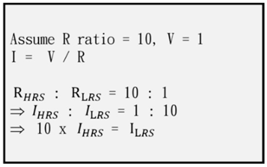
Figure 3. Example of R ratio and I_HRS vs. I_LRS.

Therefore, it can be seen that the larger the resistance on/off ratio, the more I_HRS can be tolerated in the calculation (the Current Deviation Subsection mentioned that I_HRS will cause errors). We can reduce the negative factors of the current deviation problem by using a large R ratio. However, the current range of R ratios mostly falls between 10 and 50, so this problem cannot be solved by infinitely increasing the R ratio. Furthermore, increasing the R ratio also increases the hardware area, while a small R ratio has the advantages of low leakage power, low programming cost, high density, and high retention time. It is necessary to make a trade-off between large and small R ratios without greatly affecting reliability. Taking as an example the Cifar-10 network, Figure 4 shows that the larger the R ratio, the more AWLs can be used.

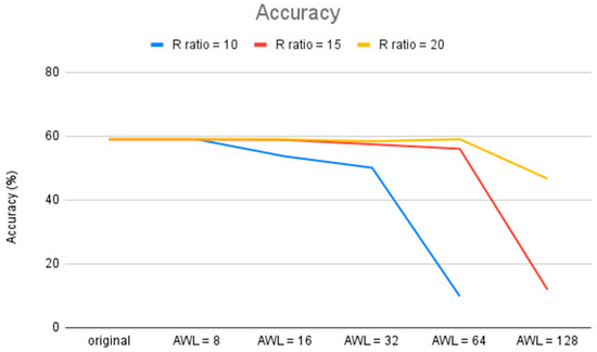
Figure 4. Accuracy of R ratio and AWL impact on Cifar-10.

2.1.3. Number of Activated Word Lines (AWLs)

In CIM computation, we can configure the number of AWLs used for calculation at a time. The larger the number of AWLs, the faster the calculation can be completed. However, due to the current deviation problem, the larger the number of AWLs, the more I_HRS is generated. In summary, the larger the number of AWLs, the larger the current deviation error is. Take Figure 5 as an example: There are three high-resistance cells and one low-resistance cell in the RRAM array on the leftmost column, and the resistance on/off ratio is 2. The example on the left activates one WL at a time, and the example on the right activates all WLs at the same time. The calculation on the left requires four computation cycles, and the result is accurate. The calculation on the right only requires one computation cycle, but the result is inaccurate. Obviously, activating one WL at a time can minimize the current deviation error, but the computation time is longer. Activating all WLs at a time can result in the fastest computational efficiency, but the generated current deviation error is the largest.

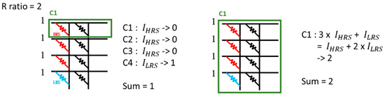
Figure 5. Example of AWL configuration on computation cycle and current deviation error.

2.2. Motivation

Due to the current deviation problem, the larger the number of AWLs, the more I_HRS is generated, and the larger the calculation error is. We can reduce the current deviation error by controlling the maximum number of AWLs to be less than the resistance on/off ratio, but from the perspective of computational efficiency, it is not a good thing. This shows that the reliability problem causes the CIM array not to be fully utilized.

By increasing the AWLs, we can effectively increase computational efficiency, but at the same time, we would reduce computational accuracy. In the example of Cifar-10 in Figure 6, when the R ratio is 10, we set the AWL number to 8 as the baseline (lower than the R ratio, so there is no current deviation error). When the AWL number is 16, the computation cycle is reduced by half, and the computational accuracy drops by 5.3%; when the AWL number is 64, the computation cycle is reduced to only one-eighth, but the computational accuracy drops to 9.85%. This shows that when the entire network uses the same number of AWLs, the scope of increasing computational efficiency is limited because of the reliability consideration.

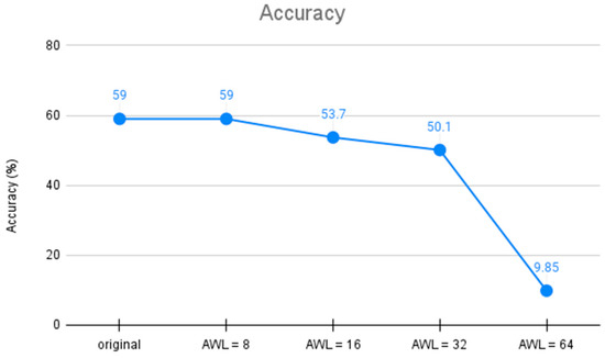
Figure 6. Impact of AWL number on accuracy with an R ratio of 10.

The adjustment of the AWLs in Figure 6 is based on the entire network; that is, all layers use the same number of AWLs. However, the number of AWLs does not have such a big impact on all layers. As shown in Figure 7, we only adjust the AWLs one layer at a time, and the other layers maintain the baseline AWLs that do not cause current deviation error. From Figure 7, we can see that the second layer of Cifar-10 is the layer most affected by the adjustment in AWLs, because this layer has the greatest number of rows in the weight matrix. In contrast, the third layer is less affected by adjusting AWLs in comparison with the second layer, because it has fewer rows in the weight matrix than the second layer. The first, fourth, and fifth layers are only slightly affected by the adjustment in AWLs because the number of rows in the weight matrix is not large in these layers. Through this experiment, we know that a layer with more rows in the weight matrix is more sensitive to the adjustment in AWLs. We can use a larger AWL configuration for the layers that are less sensitive to AWL adjustment, and a smaller AWL configuration for the layers that are sensitive to AWL adjustment.

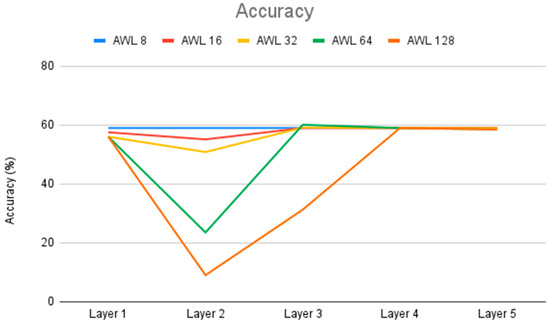
Figure 7. Accuracy of adjusting AWLs in a single layer with an R ratio of 10.

In addition, current deviation occurs when the weight bit is 0 and the IFM bit is 1. Reducing this situation can also reduce the current deviation error. Because the highest bit has the largest impact on the result, we will also use the proportion of 0 in the highest bit to adjust the AWL number. Figure 8 and Figure 9 show the proportion of 0 in the weight bits of Cifar-10 and VGG-8, respectively.

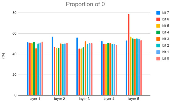
Figure 8. The proportion of 0 in the weight bits of Cifar-10.

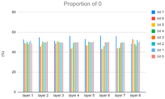
Figure 9. The proportion of 0 in the weight bits of VGG-8.

2.3. Related Works

The manuscript in [12] outlines the basic principles of computing-in-memory and the architectural design of related research, such as PRIME [13], ISAAC [5], PipeLayer [14], and PUMA [15].

In the architectural design of PRIME [13], the ReRAM-based main memory consists of a memory bank, which is divided into three areas: a storage subarray, a full-function subarray, and a buffer subarray. The storage subarray is used as a conventional storage unit, while the full-function subarray has two modes, one providing storage and the other providing computing power. The buffer subarray acts as a buffer for the computing unit, which can also be used as a conventional storage unit. A dedicated controller module parses the incoming instructions to generate the required control signals and switches the required functional subarray to the required mode. The proposed input and synapse combination scheme divides the input and synapse weights into high-order and low-order parts. Both parts are stored in separate storage units, which improves the accuracy and thus improves the overall accuracy of the artificial neural network.

In the ISAAC [5] architecture, CNNs operate in a pipelined fashion, where input values are passed through multiple layers and processed to produce an overall classification decision. ISAAC also uses a dedicated encoding scheme to reduce the size of the ADC responsible for converting the analog computation results of the memristor crossbar back into digital format and demonstrates that the performance of the computational memory accelerator is better than that of a conventional CMOS-based accelerator.

In the PipeLayer [14] architecture, the overall organization of the system is defined by a deformable subarray and a storage subarray. The former is able to switch between computing modes of storing and performing matrix–vector multiplication. PipeLayer uses a storage subarray to store intermediate results from the deformable subarrays of different layers. This reduces the amount of data movement and energy consumption, respectively. The significant improvement of this architecture comes in part from omitting the ADC and DAC according to the chosen spike scheme.

In the PUMA [15] architecture, like ISAAC, the core provides a matrix–vector multiplication unit with a memristor crossbar. The authors propose further optimizations, such as crossbar juxtaposition and input sharing (allowing multiple crossbars to use the same DAC and ADC) and input shuffling (allowing input registers to be rerouted to different DACs).

In addition to architecture design, the manuscripts in [16,17,18] propose mapping and data flow optimization techniques based on RRAM memory architecture. In order to maximize the reuse of weights and input data based on the RRAM memory architecture, the manuscript in [17] proposes a new weight mapping method and corresponding data flow which divides the kernel into different processing elements (PEs) and distributes input data to different processing elements according to their spatial location. The manuscript in [18] proposes a novel semi-folded mapping (SemiMap) framework for implementing convolution operations on crossbars. It simultaneously folds physical resources along the row dimension of the feature map (FM) and expands them along the column dimension. The former reduces the resource burden, and the latter maintains parallelism.

In recent years, the manuscript in [19] proposed a new mapping method named Squeezemapping that leverages spare space in each array and optimizes the utilization of the input dataset. The authors employed NeuroSim to simulate the inference of various networks of different scales. SSM-CIM [20] introduces a CIM macro designed for area-energy-efficient Convolutional Neural Network inference. In addition, analog computing errors and quantization errors are analyzed to ensure the multi-bit computing accuracy. The manuscript in [21] presents a bit-level sparsity method that quantizes the network to desirable numbers with more zeros in their bit representation. E-UPQ [22] presents an energy-aware unified pruning–quantization framework for the CIM architecture; it introduces a set of trainable parameters to incorporate energy information during the compression process, closing the gap between compression policy and energy optimization.

Except for the computation optimization methodology, some memristor-based DNN simulation frameworks have also been developed [23,24,25,26,27,28,29,30,31,32,33] to evaluate computational accuracy and computational efficiency. NeuroSim [26,27] is a circuit-level simulation platform that can be used to assess accelerator area, power consumption, and performance, but its architecture is not easily modified to meet our needs. MNSIM [28] offers a hierarchical modular design approach, allowing for area, power consumption, and inference accuracy assessments. However, MNSIM assesses accuracy in worst-case and average scenarios, resulting in lower accuracy than actual conditions. MemTorch [29,30] and AIHWKit [31] can support multiple types of layers and use a modular approach for hardware design. DL-RSIM [32] can simulate various factors that affect computational memory reliability. These simulation frameworks have their own areas of expertise, but they do not meet the needs of layer-wise AWL architectures. Therefore, the development of a layer-wise DNN framework based on RRAM is necessary.

Although there have been many research studies on the computation optimization of CIM [3,4,5,6,7,8,9,10,11,12,13,14,15,16,17,18,19,20,21,22], only a few of them discuss the issue of AWL configuration and its effect on computational accuracy and computational efficiency. We found that some works on RRAM-based CIM limit the maximum number of concurrent AWLs. For example, the manuscripts in [9,10] show that only 9 out of 256 word lines are activated at the same time, and the manuscript in [11] shows that only 16 out of 512 word lines are activated at the same time.

The manuscript in [3] is among the few exploring the AWL problem of CIM on inference DNN accelerators. The reported method is to first adjust the AWL number in layers for experiments (error caused by only one layer) and record the information of accuracy drop. Then the greedy algorithm is used to select the layer and AWL number that causes the smallest error, and then, experiments are conducted to evaluate accuracy. Only one layer is selected for adjustment in each round until accuracy drops beyond the set threshold. However, this method requires multiple experiments to determine the AWL configuration for each layer, and the authors do not consider the proportion of 0 in weight bits as described above.

Due to these issues, in this paper, we propose a methodology to configure a suitable AWL size for each layer according to the features of the neural network (length of weight matrix, layer type, etc.), the R ratio, and other aspects. While increasing computational efficiency, we also consider the maintenance of computational accuracy. In addition, we also develop a layer-wise CIM simulation framework to evaluate the accuracy and efficiency of the proposed methodology in the inference stage.

3. Proposed Framework and Methodology

Overall, our framework follows the methodology, architecture, and parameters of NeuroSim. The purpose of the proposed framework is to verify our AWL configuration method and exploring different AWL configurations. In this section, we describe our inference accuracy predictor, quantization and current deviation error calculation methods, and the layer-wise AWL decision methodology. The proposed risk factors and index mapping methods are easy to fine-tune for future extension and exploration.

3.1. Inference Accuracy Predictor

Current simulation tools for RRAM CIM rarely consider the impact of layer-wise AWL configuration on computational accuracy. Therefore, based on our layer-wise AWL configuration method, the current deviation and R ratio factors that affect RRAM CIM accuracy, and the proposed quantization and current deviation error calculation methods in Section 3.1 and Section 3.2, we develop an inference accuracy predictor. Our prediction model is based on the inference estimation algorithm of NeuroSim [26,27], and we adapt the same synaptic array architecture and circuit parameters. The main difference is that the AWL number is fixed for all neural layers in NeuroSim, while our accuracy predictor calculates accuracy based on our layer-wise AWL configuration, and quantization and current deviation error calculation methods.

In this framework, the neural network model (or weights) is assumed to be pre-trained by software and then mapped to the inference CIM array. As shown in Figure 10, our predictor receives weights, a neural network model, a test dataset, and hardware constraints. We quantize the input weights and IFMs to a specified range based on the DAC precision within the input hardware constraints. These quantized weights and IFMs serve as inputs to the CIM array. The CIM array first maps the input weights to the array, representing them as high–low configurations. The IFMs are input as voltages from the WL direction and are calculated in batches based on the dynamic AWL configuration specified in the hardware constraints. The output is expressed as current, which includes current deviation. Finally, the inference model converts the CIM output current into a calculated result based on the R ratio and ADC precision within the hardware constraints. After the inference model is calculated, the predicted answer is compared with the real result.

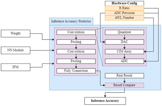
Figure 10. Architecture of inference accuracy predictor.

With this accuracy predictor, we can analyze the impact of different AWL configuration methods on the inference accuracy.

3.2. Quantization Method

In CNN computations, weights and IFMs are typically stored as floating-point numbers. To conserve hardware resources and increase computational efficiency, the original values are typically quantized to reduce the number of bits required to represent them.

In the proposed inference accuracy predictor, we use a linear transformation method to convert weight and IFMs to the specified interval. For the example of 8-bit quantization, Formula (1) shows that since the weight range is [−1, 1], the weight is converted from a floating-point number between [−1, 1] to an integer between [−128, 127]. Because the input feature map does not have a clear range, we use the maximum and minimum values as the range boundaries for conversion; that is, we convert [IFM minimum, IFM maximum] into [0, 255], as shown in Formula (2).

In the convolutional computation, we add 128 to the converted weight, so the weight conversion range becomes [0, 255]. The additional 128 will be deducted after the calculation is completed and will not affect the result. As shown in Figure 11, we can simply deduct Σ(Ai × 128) after the calculation without affect the computing result. This allows us to avoid the need for considering the positive and negative signs during the calculation process.

$$W_q={\displaystyle \frac{W-(-1)}{1-(-1)}}\ast \left(127-\left(-128\right)\right)+(-128)$$

(1)

$${IFM}_q={\displaystyle \frac{IFM-\left(min\right)}{max-\left(min\right)}}\ast 255$$

(2)

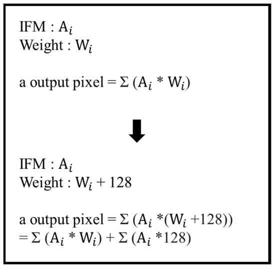
Figure 11. Derivation of weight quantization.

Figure 12 shows the weight distribution of Cifar-10. We can observe that the weight distribution exhibits a normal distribution, with most weights being concentrated around 0 (the center) and the weight distribution decreasing towards either side. Therefore, during quantization, we narrow the weight range from [−1, 1] to [−0.8, 0.8]. Weights larger than 0.8 are stored as 0.8, and weights smaller than −0.8 are stored as −0.8. By quantizing within a narrow range, we can create larger disparity between weights in the densely populated middle range, thereby improving accuracy. Formula (3) is the final weight quantification equation.

$$W_q={\displaystyle \frac{W-(-0.8)}{0.8-(-0.8)}}\ast \left(127-\left(-128\right)\right)+\left(-128\right)+128)$$

(3)

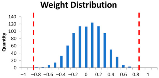
Figure 12. Weight distribution of Cifar-10.

3.3. Current Deviation Error Calculation

Overall, our custom simulator follows the architecture and parameters of NeuroSim, and we only modify the calculation of current deviation error. To calculate the current error, we need to compute it in bits, but this is very inefficient. So, we compute the correct result and the current error separately to speed up the simulation, as shown in Figure 13. The correct result is calculated as in Keras, multiplying the weights and the IFM and accumulating them. The current error is calculated by accumulating the number along the BLs with a weight of 0 and an IFM of 1. It is calculated in batches according to the AWLs, converted into a value, and then added to the correct result and stored. We use this approach to avoid performing accurate numerical calculations at the bit level and to discard the numerical conversion of the current of the high-configuration computing memory unit that does not cause errors.

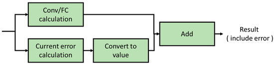
Figure 13. Convolutional layer and fully connected layer error calculation process.

3.4. Layer-Wise AWL Decision Methodology

In our research, several factors influence the AWL configuration, as we illustrate below, and these four observations are collectively called risk factors:

• The first one is the size of the R ratio. The larger the R ratio, the larger the current error that can be tolerated in the calculation.
• The second one is the type of neural network layer. Convolutional layers require higher accuracy because they are typically ranked earlier. If accuracy is lost early in the computation, subsequent layers are more likely to experience worse accuracy. Fully connected layers are typically ranked later, so a larger AWL number can be used for these layers.
• The third one is the number of expanded weight rows. This represents the number of dot products that need to be accumulated for one output pixel. A larger value indicates that more rows need to be accumulated, which in turn means a large potential for accumulated current deviation.
• The last one is the proportion of 0 in the MSB. A higher proportion of 0 indicates a higher number of high-configuration computing memory cells, which increases the probability of current error.

Table 1 shows the risk factors and their impact value on the risk index. We calculate the risk index layer by layer according to the characteristics of each layer. Initially the risk index of each layer is 0, and the final risk index of a layer is obtained by summing its corresponding impact values. Among the risk factors, except for the matrix rows, we consider all other risk factors to be equally important, and their impact values are ±1, as shown in Table 1. Therefore, for a convolutional layer, we increase its risk index by one, while for an FC layer, we decrease its risk index by one; if the ratio of 0 in the MSB is large enough in a layer, we also increase its risk index by one; if the R ratio is small, we will increase the risk index of all layers by one, and vice versa. Finally, we observe that the size span of the matrix rows is large, so we calculate its impact value by ${\lfloor log}_{2}Row-7\rfloor$.

Table 1. Risk factors and their impact values on risk index.

Risk Factor	Impact Value
R Ratio <= 10	+1
Convolutional Layer	+1
Matrix Row (R) >= 256	+${\lfloor log}_{2}R-7\rfloor$
Ratio of 0 in MSB >= 55%	+1
R Ratio >= 20	−1
(FC(Dense) Layer|| Next Layer = FC Layer) && R Ratio > 10	−1

For each layer, the selected AWL size is based on its risk index. The larger the risk index, the larger the error that may occur, so a small AWL number should be used to reduce the error. On the contrary, a large AWL number can be used for layers with a smaller risk index. The corresponding mapping is shown in Table 2.

Table 2. Risk index and corresponding AWL mapping.

Risk Index	AWLs
>3 (ratio <= 10)	8
>=3	16
2	32
1	64
<=0	128

We summarize the reasons why except for matrix rows, the impact values of all other risk factors are ±1 as follows:

• In our observation, the R ratio of 10 is a threshold, and accuracy is very sensitive to the AWL configuration when R ratio <= 10. Therefore, we isolate this item as a risk factor.
• An R ratio of 20 is a middle value, accuracy is not so sensitive to the AWL configuration when the R ratio >= 20; therefore, we also isolate it as a risk factor.
• For the ratio of 0 in the MSB, we also observe that 55% is a middle and suitable value. Almost no layers reach the threshold if we increase this value to 60%, and too many layers reach the threshold if we decrease this value to 50%.
• One only needs to identify whether the layer type is convolution or fully connected.
• Over-emphasizing the importance of one risk factor will reduce the effect of other risk factors, so we set the impact values of all the above risk factors to ±1.

Finally, we summarize the directions to fine-tune risk factors and risk indexes for large neural network architectures and large R ratios to increase computational efficiency without sacrificing too much accuracy:

• For large neural network architectures, most layers will satisfy the threshold of the matrix row risk factor. In order to increase computational efficiency when the R ratio <= 20, one direction is to increase this risk factor threshold. For example, we can change the matrix row risk factor from R >= 256 to R >= 512, and the impact value calculation is modified from +${\lfloor log}_{2}R-7\rfloor$ to +${\lfloor log}_{2}R-8\rfloor$. By this tuning, more neural layers have the opportunity to increase their AWL number.
• For large R ratios, more current error can be tolerated in the calculation. Therefore, one direction to increase computational efficiency when R > 20 is to increase the mapping AWLs in the risk index table. For example, when the value of the risk index is 3, we can change the AWL mapping from 16 to 32, etc. By this tuning, most neural layers can increase their AWL number.

4. Evaluation Results

4.1. Experimental Setup

We verify our methodology on Cifar-10 [34], VGG-8 [35], and ResNet-18 [36] and use the proposed RRAM accuracy predictor to simulate inference accuracy and computational efficiency.

Since our target is an efficient layer-wise AWL configuration methodology but not an improved CIM circuit architecture design, we adapt the same synaptic array architecture and circuit parameters from NeuroSim [26,27]; the hardware behavior (such as power, latency, and area) is also similar to that of NeuroSim. Therefore, we focus on comparing the inference accuracy and computation cycles of different AWL configurations in the experimental results.

The CIM hardware settings used in the experiments are shown in Table 3. We use a 512 × 512 CIM array based on RRAM, where each RRAM cell represents 1-bit data, and the ADC precision is 8 bits. We analyze the relationship between inference accuracy and computational efficiency for different AWL configurations and R ratios.

Table 3. CIM hardware settings.

Simulator	RRAM Accuracy Predictor
CNN	Cifar-10, VGG-8, ResNet-18
CIM Array Size	512 × 512
RRAM Cell	1 bit/pre cell
R Ratio	10, 15, 20, 25, 35
ADC Precision	8 bit

The network architectures of Cifar-10, VGG-8, and ResNet-18 and their layer-wise risk index and AWL mapping based on our AWL decision methodology are described below.

4.1.1. Cifar-10

Table 4 lists the Cifar-10 network architecture and ratio of 0 in the MSB; matrix row is the number of rows of the weight matrix, and its formula is ${Kernel}^2\ast Channel$, while matrix col. is Depth. We calculate the risk index of each layer based on the impact values of the risk factors in Table 1, and the results are shown in Table 5.

Table 4. Cifar-10 network architecture and ratio of 0 in MSB.

	Layer Type	Input	Channel	Kernel	Depth	Matrix Row	Matrix Col.	Ratio of 0 in MSB
Layer 1	Conv	32	3	3	32	27	32	51.39%
Layer 2	Conv	15	32	5	64	800	64	57%
Layer 3	Conv	3	64	3	64	576	64	56.18%
Layer 4	Dense	1	64	1	64	64	64	52.59%
Layer 5	Dense	1	64	1	10	64	10	53.28%

Table 5. Cifar-10 layer-wise risk index and AWL mapping.

	Risk Index			AWL
R Ratio	10	15	20	10	15	20
Layer 1	2	1	0	32	32	32
Layer 2	5	4	3	8	16	16
Layer 3	5	3	2	8	16	32
Layer 4	1	−1	−2	64	64	64
Layer 5	1	−1	−2	64	64	64

Take the second layer with an R ratio of 15 as an example: The risk factors of the second layer include (1) layer type: convolution; (2) matrix ow (R) >= 256; and (3) ratio of 0 in the MSB >= 55%. Therefore, the risk index is (1) + (2) + (3) = 1 + ⌊log2800 − 7⌋ + 1 = 4. After calculating the risk index and referring to Table 2, we find that the AWL number is 16 for the second layer with an R ratio of 15. The AWL of the first layer with an R ratio of 15 is 32, instead of 64, as shown in Table 5; this is because the matrix row of the first layer is only 27, and 32 AWLs at a time are enough for full calculation. The same reason is also applied to the AWLs of the first layer with an R ratio of 20, and the last two layers with R ratios of 15 and 20, respectively.

4.1.2. VGG-8

Table 6 and Table 7 list the VGG-8 network architecture, with ratio of 0 in the MSB, the risk index, and the AWL number of each layer. Taking layer 7 with an R ratio of 15 as an example, the risk factors include (1) matrix row (R) >= 256, (2) a ratio of 0 in the MSB >= 55%, and (3) the layer type of fully connected and an R ratio > 10. The risk index is calculated as (1) + (2) + (3) = ${\lfloor log}_{2}2048-7\rfloor +1-1=4$. Referring to Table 2, we see that the AWL number of layer 7 is 16.

Table 6. VGG-8 network architecture and ratio of 0 in MSB.

	Layer Type	Input	Channel	Kernel	Depth	Matrix Row	Matrix Col.	Ratio of 0 in MSB
Layer 1	Conv	32	3	3	32	27	32	52.78%
Layer 2	Conv	32	32	3	32	288	32	54.83%
Layer 3	Conv	16	32	3	64	288	64	51.54%
Layer 4	Conv	16	64	3	64	576	64	56.31%
Layer 5	Conv	8	64	3	128	576	128	53.25%
Layer 6	Conv	8	128	3	128	1152	128	56.76%
Layer 7	Dense	1	2048	1	128	2048	128	56.02%
Layer 8	Dense	1	128	1	10	128	10	48.67%

Table 7. VGG-8 layer-wise risk index and AWL mapping.

	Risk Index			AWL
R Ratio	10	15	20	10	15	20
Layer 1	2	1	0	32	32	32
Layer 2	3	2	1	16	32	64
Layer 3	3	2	1	16	32	64
Layer 4	5	4	3	8	16	16
Layer 5	4	3	2	8	16	32
Layer 6	6	4	3	8	16	16
Layer 7	6	4	3	8	16	16
Layer 8	1	−1	−2	64	128	128

4.1.3. ResNet-18

Table 8 lists the ResNet-18 network architecture with a ratio of 0 in the MSB, and Table 9 lists the risk index and AWLs of each layer. Because the matrix row of most layers is larger than 256, in addition to the risk factor $Matrix Row \left(R\right) >= 256$, Table 9 also lists the risk index and AWLs when this risk factor is changed to $Matrix Row \left(R\right) >= 512$.

Table 8. ResNet-18 network architecture and ratio of 0 in MSB.

	Layer Type	Input	Channel	Kernel	Depth	Matrix Row	Matrix Col.	Ratio of 0 in MSB
Layer 1	Conv	224	3	7	64	147	64	52.38%
Layer 2	Conv	56	64	3	64	576	64	54.61%
Layer 3	Conv	56	64	3	64	576	64	53.82%
Layer 4	Conv	56	64	3	64	576	64	54.43%
Layer 5	Conv	56	64	3	64	576	64	54.12%
Layer 6	Conv	56	64	3	128	576	128	55.71%
Layer 7	Conv	28	128	3	128	1152	128	54.32%
Layer 8	Conv	56	64	1	128	64	128	53.37%
Layer 9	Conv	28	128	3	128	1152	128	53.79%
Layer 10	Conv	28	128	3	128	1152	128	54.83%
Layer 11	Conv	28	128	3	256	1152	256	56.68%
Layer 12	Conv	14	256	3	256	2304	256	53.64%
Layer 13	Conv	28	128	1	256	128	256	54.77%
Layer 14	Conv	14	256	3	256	2304	256	55.17%
Layer 15	Conv	14	256	3	256	2304	256	52.65%
Layer 16	Conv	14	256	3	512	2304	512	51.37%
Layer 17	Conv	7	512	3	512	4608	512	53.44%
Layer 18	Conv	14	256	1	512	256	512	54.62%
Layer 19	Conv	7	512	3	512	4608	512	56.76%
Layer 20	Conv	7	512	3	512	4608	512	52.08%
Layer 21	Dense	1	512	1	1000	512	1000	50.32%

Table 9. ResNet-18 layer-wise risk index and AWL mapping.

	Risk Index						AWL
	R >= 256			R >= 512			R >= 256			R >= 512
R Ratio	10	15	20	10	15	20	10	15	20	10	15	20
Layer 1	2	1	0	2	1	0	32	64	128	32	64	128
Layers 2~5	4	3	2	3	2	1	8	16	32	16	32	64
Layers 6~7	5	4	3	4	3	2	8	16	16	8	16	32
Layer 8	2	1	0	2	1	0	32	64	64	32	64	64
Layers 9~10	5	4	3	4	3	2	8	16	16	8	16	32
Layers 11~12	6	5	4	5	4	3	8	16	16	8	16	16
Layer 13	2	1	0	2	1	0	32	64	128	32	64	128
Layer 14	7	6	5	6	5	4	8	16	16	8	16	16
Layers 15~16	6	5	4	5	4	3	8	16	16	8	16	16
Layer 17	7	6	5	6	5	4	8	16	16	8	16	16
Layer 18	3	2	1	2	1	0	16	32	64	32	64	128
Layer 19	8	7	6	7	6	5	8	16	16	8	16	16
Layer 20	7	5	4	6	4	3	8	16	16	8	16	16
Layer 21	3	1	0	2	0	−1	16	64	128	32	128	128

4.2. Analysis of Accuracy and Efficiency for Small R Ratios

Small R ratios have a more serious impact on the generated current error. Therefore, we firstly use R ratios of 10, 15, and 20 to discuss the effect of the AWL configuration on accuracy and efficiency. Besides with the baseline, we also compare our layer-wise AWL decision methodology with the fixed-AWL configuration (Fix 16).

4.2.1. Cifar-10

Table 10 lists the AWL configuration of each layer, accuracy, and the cycle count with different R ratios; we use the quantified accuracy, which is 59%, as the baseline. Compared with the “Fix 16” configuration, our methodology has better accuracy with an R ratio of 10 and has better computational efficiency with R ratios of 15 and 20. Figure 14 shows the accuracy comparison with different R ratios.

Table 10. Accuracy and total cycles of Cifar-10 using fixed AWLs and layer-wise AWLs.

	AWL
R Ratio	Baseline	10		15		20
		Fix 16	Ours	Fix 16	Ours	Fix 16	Ours
Layer 1	8	16	32	16	32	16	32
Layer 2	8	16	8	16	16	16	16
Layer 3	8	16	8	16	16	16	32
Layer 4	8	16	64	16	64	16	64
Layer 5	8	16	64	16	64	16	64
ACC	59%	53.7%	55.65%	57.2%	57.2%	58.35%	58.35
ACC Loss	X	−5.3%	−3.35%	−1.8%	−1.8%	−0.65%	−0.65%
Total Cycles	192	96	175	96	89	96	71
Cycle Benefit	X	−50%	−9%	−50%	−54%	−50%	−63%

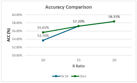
Figure 14. Accuracy comparison of Cifar-10 for different R ratios.

4.2.2. VGG-8

Table 11 lists the AWL configuration of each layer, accuracy, and the cycle count for different R ratios, where the baseline accuracy is 64.9%. We have similar comparison results for VGG-8 with respect to Cifar-10.

Table 11. Accuracy and total cycles of VGG-8 using fixed AWLs and layer-wise AWLs.

	AWL
R Ratio	Baseline	10		15		20
		Fix 16	Ours	Fix 16	Ours	Fix 16	Ours
Layer 1	8	16	32	16	32	16	32
Layer 2	8	16	16	16	32	16	64
Layer 3	8	16	16	16	32	16	64
Layer 4	8	16	8	16	16	16	16
Layer 5	8	16	8	16	16	16	32
Layer 6	8	16	8	16	16	16	16
Layer 7	8	16	8	16	16	16	16
Layer 8	8	16	64	16	128	16	128
ACC	64.9%	60.15%	62%	63.9%	63.9%	64.79%	64.79%
ACC Loss	X	−4.75%	−2.9%	−1%	−1%	−0.11%	−0.11%
Total Cycles	1108	554	1055	554	528	554	484
Cycle Benefit	X	−50%	−5%	−50%	−52%	−50%	−56%

4.2.3. ResNet-18

Table 12 lists the AWL configuration of each layer, accuracy, and the cycle count for different R ratios, where the baseline accuracy is 71.6%. Because the matrix row factor of most layers is larger than 256, in addition to the original risk factor $Matrix Row \left(R\right) >= 256$, we also list the results when this risk factor is changed to $Matrix Row \left(R\right) >= 512$.

Table 12. Accuracy and total cycles of ResNet-18 using fixed AWLs and layer-wise AWLs.

	AWL
R Ratio	Baseline	10			15			20
		Fix 16	R256	R512	Fix 16	R256	R512	Fix 16	R256	R512
Layer 1	8	16	32	32	16	64	64	16	128	128
Layers 2~5	8	16	8	16	16	16	32	16	32	64
Layers 6~7	8	16	8	8	16	16	16	16	16	32
Layer 8	8	16	32	32	16	64	64	16	128	128
Layers 9~12	8	16	8	8	16	16	16	16	16	16
Layer 13	8	16	32	32	16	64	64	16	128	128
Layers 14~17	8	16	8	8	16	16	16	16	16	16
Layer 18	8	16	16	32	16	32	64	16	64	128
Layers 19~20	8	16	8	8	16	16	16	16	16	16
Layer 21	8	16	16	32	16	64	128	16	128	128
ACC	71.6%	62.5%	69.2%	68.3%	69.9%	69.9%	69.88%	70.8%	70.75%	70.72%
ACC Loss	X	−9.1%	−2.4%	−3.3%	−1.7%	−1.7%	−1.72%	−0.8%	−0.85%	−0.88%
Total Cycles	3955	1978	3875	3707	1978	1930	1850	1978	1848	1756
Cycle Benefit	X	−50%	−2%	−6.3%	−50%	−51.2%	−53.2%	−50%	−53.3%	−55.6%

We have similar comparison results on VGG-18 with respect to Cifar-10 and VGG-8. Comparing the modified risk factor (R512) with the original risk factor (R256), a small increaser in computational efficiency is achieved with little loss in accuracy.

4.2.4. Discussion

The experiments on Cifar-10, VGG-8, and ResNet-18 all show that compared with the “Fix 16” configuration, our methodology has better accuracy with an R ratio of 10 and has better computational efficiency with R ratios of 15 and 20.

The experimental results also show that computational accuracy is much more sensitive to the AWL configuration for the R ratio of 10 compared with R ratios of 15 and 20. Because of special consideration for the R ratio of 10 in the risk factors, our methodology has less accuracy reduction with an R ratio of 10, while for R ratios of 15 and 20, because the larger the R ratio, the more current deviations can be tolerated, computational accuracy is less sensitive to the AWL configuration, and our methodology has the best computational efficiency with very little accuracy reduction. Overall, our methodology performs the best in terms of computational accuracy and computational efficiency for an R ratio of 20; the experimental results illustrate the advantage of our layer-wise AWL decision method and special risk factor design.

Finally, for the application of our methodology to ResNet-18, because the matrix row factor of most layers is larger than 256, a modified risk factor further reduces the cycle count a little with little accuracy loss in comparison with the original risk factor. This shows that for large neural network architectures, tuning on our risk factors is easy and offers a flexible space for a trade-off between computational accuracy and computational efficiency.

4.3. Exploration on Large R Ratio and AWL Size

4.3.1. Risk Index and AWL Mapping

In our risk factor design, R ratios of 25 and 35 have the same risk index as the R ratio of 20. In addition, the larger the R ratio, the larger the minimal AWLs can be used. Therefore, for R ratios of 25 and 35, the minimal AWLs can be increased from 16 to 32 or even more. Therefore, except for the original risk index and AWL mapping for small R ratios (min. AWL = 16), Table 13 lists the mapping of risk index and different minimal AWLs for R ratios of 25 and 35.

Table 13. Risk index and different Min. AWL mapping table for R ratios of 25 and 35.

	AWLs
Risk Index	Min. AWL = 16	Min. AWL = 32	Min. AWL = 64	Min. AWL = 128	Min. AWL = 256
>=3	16	32	64	128	256
2	32	64	128	256	512
1	64	128	256	512	512
<=0	128	256	512	512	512

4.3.2. Results

In Table 14, Table 15 and Table 16, we list the accuracy and cycle benefit on Cifar-10, VGG-8, and ResNet-18, with different minimal AWLs for R ratios of 25 and 35. Figure 15 shows the accuracy comparison of ResNet-18 for different Min. AWLs.

Table 14. Accuracy and cycle benefit of Cifar-10 for different Min. AWLs for R ratios of25 and 35.

	AWLs
Min. AWL	16	32	64	128	256
Layer 1	32	32	32	32	32
Layer 2	16	32	64	128	256
Layer 3	32	64	128	256	512
Layer 4	64	64	64	64	64
Layer 5	64	64	64	64	64
ACC—R Ratio 25	59%	59%	58.9%	59.65%	21.14%
ACC—R Ratio 35	59%	59%	59%	59.15%	51.83%
ACC Loss—R Ratio 25	−0%	−0%	−0.1%	+0.65%	−37.86%
ACC Loss—R Ratio 35	−0%	−0%	−0%	+0.15%	−7.17%
Total Cycles	71	37	21	12	8
Cycle Benefit	−63%	−81%	−89%	−93%	−95%

Table 15. Accuracy and cycle benefit of VGG-8 for different Min. AWLs for R ratios of 25 and 35.

	AWLs
Min. AWL	16	32	64	128	256
Layer 1	32	32	32	32	32
Layer 2	64	128	256	512	512
Layer 3	64	128	256	512	512
Layer 4	16	32	64	128	256
Layer 5	32	64	128	256	512
Layer 6	16	32	64	128	256
Layer 7	16	32	64	128	256
Layer 8	128	128	128	128	128
ACC—R Ratio 25	64.9%	64.85%	64.1%	61.8%	44.25%
ACC—R Ratio 35	64.9%	64.9%	64.8%	63.1%	55.3%
ACC Loss—R Ratio 25	−0%	−0.05%	−0.8%	−3.1%	−20.65%
ACC Loss—R Ratio 35	−0%	−0%	−0.1%	−1.8%	−9.6%
Total Cycles	484	244	124	64	55
Cycle Benefit	−56%	−78%	−89%	−94%	−95%

Table 16. Accuracy and cycle benefit of ResNet-18 for different Min. AWLs for R ratios of 25 and 35.

	AWLs
Min. AWL	16	32	64	128	256
Layer 1	128	256	256	256	256
Layers 2~5	32	64	128	256	512
Layers 6~7	16	32	64	128	256
Layer 8	64	64	64	64	64
Layers 9~10	16	32	64	128	256
Layers 11~12	16	32	64	128	256
Layer 13	128	128	128	128	128
Layer 14	16	32	64	128	256
Layers 15~16	16	32	64	128	256
Layer 17	16	32	64	128	256
Layer 18	64	128	256	256	256
Layer 19	16	32	64	128	256
Layer 20	16	32	64	128	256
Layer 21	128	256	512	512	512
ACC—R Ratio 25	71.2%	71.05%	70.6%	67.1%	41.8%
ACC—R Ratio 35	71.6%	71.5%	71.2%	69.8%	60.2%
ACC Loss—R Ratio 25	−0.4%	−0.55%	−1%	−4.5%	−29.8%
ACC Loss—R Ratio 35	−0%	−0.1%	−0.4%	−1.8%	−11.4%
Total Cycle	1848	925	466	238	193
Cycle Benefit	−53.3%	−76.6%	−88.2%	−94%	−95%

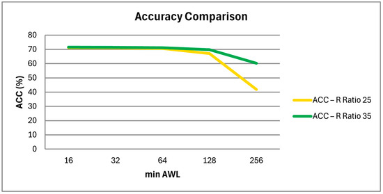
Figure 15. Accuracy comparison of ResNet-18 for different Min. AWLs.

4.3.3. Discussion

The experiments on Cifar-10, VGG-8, and ResNet-18 all show that when the minimal AWL number is increased from 16 to 32 or 64, there is only a small accuracy reduction, but there is a large computation cycle benefit. The reason is also because the larger the R ratio, the more current deviations can be tolerated; therefore, computational accuracy is less sensitive to the AWL configuration.

However, when the minimal AWL number is increased to 128, accuracy begins to have an obvious reduction for VGG-8 and ResNet-18, especially with an R ratio of 25. But for Cifar-10, we speculate that the slight increase in accuracy is due to the fact that the error introduced by this configuration just causes some data that the original model had previously misjudged to be correct, and we believe that it is a special case.

In addition, all three tables show a significant drop in accuracy when the minimal AWL number is increased to 256. Therefore, we can conclude that for R ratios of 25 and 35, increasing the minimal AWL number from 16 to 32 or 64 yields the best results.

From the experimental results, we know that increasing the R ratio can improve the problem of declining accuracy and allows us to use a larger AWL number and achieve better computational efficiency. However, the current range of R ratios mostly falls between 10 and 50, so this problem cannot be solved by infinitely increasing the R ratio. Furthermore, increasing the R ratio also increases the hardware area, which is a burden for devices with limited size. For our methodology, increasing the R ratio to 25 or 35 allows us to have a more flexible planning space and better computational efficiency.

5. Conclusions

In this paper, we propose a layer-wise AWL strategy to configure the appropriate number of AWLs for each neural layer. Our AWL configuration also takes into account the effect of the resistance on/off ratio (R ratio); based on the observed risk factors, we design a risk index-to-AWL mapping methodology. Meanwhile, based on the proposed quantization and current deviation error calculation methods, we design a CIM simulation framework to simulate the accuracy of CNNs in the inference stage.

The proposed methodology improves computational efficiency with only slight accuracy loss. In comparison with the fixed-AWL configuration, our methodology has better computational accuracy with small resistance on/off ratios. For higher resistance on/off ratios, our methodology shows a significant improvement in computational efficiency in comparison with the baseline. On the exploration of different R ratios, experimental results show that our layer-wise AWL configuration methodology has a more flexible planning space and better computational efficiency.

In a future perspective, extending our work to study the sensitivity of cell resistance deviation is the key direction. In this paper, we explore our methodology on the sensitivity of current deviation and resistance on/off ratio, but cell resistance deviation is another important factor that has a great impact on computational accuracy and computational efficiency of RRAM CIM. However, integrating these three sensitivity problems together is complex, and more observation and study are necessary.

In addition to cell resistance deviation, other RRAM non-idealities, such as IR drop and ADC noise, are all important issues that lead to a non-linear relationship between computational accuracy and computational efficiency. To overcome these challenges, enhanced risk factor designs and more flexible index mapping methods are necessary, which are important future directions of our work.

References

- Lecun, Y.; Bengio, Y.; Hinton, G. Deep learning. Nature 2015, 521, 436–444. [Google Scholar] [CrossRef] [PubMed]
- Krizhevsky, A.; Sutskever, I.; Hinton, G. ImageNet Classification with Deep Convolutional Neural Networks. In Proceedings of the Neural Information and Processing Systems (NIPS), Lake Tahoe, NV, USA, 3–8 December 2012. [Google Scholar]
- Park, Y.; Lee, S.Y.; Shin, H.; Heo, J.; Ham, T.J.; Lee, J.W. Unlocking Wordline-level Parallelism for Fast Inference on RRAM-based DNN Accelerator. In Proceedings of the 39th International Conference on Computer-Aided Design (ICCAD), San Diego, CA, USA, 2–5 November 2020. [Google Scholar]
- Verma, N.; Jia, H.; Valavi, H.; Tang, Y.; Ozatay, M.; Chen, L.Y.; Zhang, B.; Deaville, P. In-Memory Computing: Advances and prospects. IEEE Solid-State Circuits Mag. 2019, 11, 43–55. [Google Scholar] [CrossRef]
- Shafiee, A.; Nag, A.; Muralimanohar, N.; Balasubramonian, R.; Strachan, J.P.; Hu, M.; Williams, R.S.; Srikumar, V. ISAAC: A Convolutional Neural Network Accelerator with In-Situ Analog Arithmetic in Crossbars. In Proceedings of the 43rd International Symposium on Computer Architecture (ISCA), Seoul, Republic of Korea, 18–22 June 2016. [Google Scholar]
- Wong, H.S.P.; Lee, H.Y.; Yu, S.; Chen, Y.S.; Wu, Y.; Chen, P.S.; Lee, B.; Chen, F.T.; Tsai, M.J. Metal–Oxide RRAM. Proc. IEEE 2012, 100, 1951–1970. [Google Scholar] [CrossRef]
- Hu, M.; Strachan, J.P.; Li, Z.; Grafals, E.M.; Davila, N.; Graves, C.; Lam, S.; Ge, N.; Yang, J.J.; Williams, R.S. Dot-product engine for neuromorphic computing: Programming 1T1M crossbar to accelerate matrix-vector multiplication. In Proceedings of the 53rd ACM/EDAC/IEEE Design Automation Conference (DAC), Austin, TX, USA, 5–9 June 2016. [Google Scholar]
- Feinberg, B.; Wang, S.; Ipek, E. Making Memristive Neural Network Accelerators Reliable. In Proceedings of the IEEE International Symposium on High Performance Computer Architecture (HPCA), Vienna, Austria, 24–28 February 2018. [Google Scholar]
- Chen, W.H.; Li, K.X.; Lin, W.Y.; Hsu, K.H.; Li, P.Y.; Yang, C.H.; Xue, C.X.; Yang, E.Y.; Chen, Y.K.; Chang, Y.S.; et al. A 65nm 1Mb nonvolatile computing-in-memory ReRAM macro with sub-16ns multiply-and-accumulate for binary DNN AI edge processors. In Proceedings of the IEEE International Solid-State Circuits Conference (ISSCC), San Francisco, CA, USA, 11–15 February 2018. [Google Scholar]
- Xue, C.X.; Chen, W.H.; Liu, J.S.; Li, J.F.; Lin, W.Y.; Lin, W.E.; Wang, J.H.; Wei, W.C.; Chang, T.W.; Chang, T.C.; et al. A 1Mb Multibit ReRAM Computing-In-Memory Macro with 14.6ns Parallel MAC Computing Time for CNN Based AI Edge Processors. In Proceedings of the IEEE International Solid-State Circuits Conference (ISSCC), San Francisco, CA, USA, 17–21 February 2019. [Google Scholar]
- Xue, C.X.; Huang, T.Y.; Liu, J.S.; Chang, T.W.; Kao, H.Y.; Wang, J.H.; Liu, T.W.; Wei, S.Y.; Huang, S.P.; Wei, W.C.; et al. A 22nm 2Mb ReRAM Compute-in-Memory Macro with 121–28TOPS/W for Multibit MAC Computing for Tiny AI Edge Devices. In Proceedings of the IEEE International Solid-State Circuits Conference (ISSCC), San Francisco, CA, USA, 16–20 February 2020. [Google Scholar]
- Staudigi, F.; Merchant, F.; Leupers, R. A survey of Neuromorphic Computing-in-Memory: Architectures, Simulators and Security. IEEE Des. Test 2021, 39, 90–99. [Google Scholar] [CrossRef]
- Chi, P.; Li, S.; Qi, Z.; Gu, P.; Xu, C.; Zhang, T.; Zhao, J.; Liu, Y.; Wang, Y.; Xie, Y. PRIME: A Novel Processing-In-Memory Architecture for Neural Network Computation in ReRAM-based Main Memory. In Proceedings of the 43rd International Symposium on Computer Architecture (ISCA), Seoul, Republic of Korea, 18–22 June 2016. [Google Scholar]
- Song, L.; Qian, X.; Li, H.; Chen, Y. Pipelayer: A pipelined reram-based accelerator for deep learning. In Proceedings of the IEEE International Symposium on High Performance Computer Architecture (HPCA), Austin, Texas, USA, 4–8 February 2017. [Google Scholar]
- Ankit, A.; Hajj, I.E.; Chalamalasetti, S.R.; Ndu, G.; Foltin, M.; Williams, R.S.; Faraboschi, P.; Hwu, W.; Strachan, J.P.; Roy, K.; et al. PUMA: A Programmable Ultra-efficient Memristor-based Accelerator for Machine Learning Inference. arXiv 2019, arXiv:1901.10351. [Google Scholar]
- Gokmen, T.; Onen, M.; Haensch, W. Training deep convolutional neural networks with resistive cross-point devices. Neuroscience 2017, 11, 538. [Google Scholar] [CrossRef] [PubMed]
- Peng, X.; Liu, R.; Yu, S. Optimizing Weight Mapping and Data Flow for Convolutional Neural Networks on RRAM based Processing-In-Memory Architecture. In Proceedings of the IEEE International Symposium on Circuits and Systems (ISCAS), Sapporo, Japan, 26–29 May 2019. [Google Scholar]
- Deng, L.; Liang, L.; Wang, G.; Chang, L.; Hu, X.; Ma, X.; Liu, L.; Pei, J.; Li, G.; Xie, Y. SemiMap: A Semi-Folded Convolution Mapping for Speed-Overhead Balance on Crossbars. IEEE Trans. Comput.-Aided Des. Integr. Circuits Syst. 2020, 39, 117–130. [Google Scholar] [CrossRef]
- Wang, S.; Liang, F.; Cao, Q.; Wang, Y.; Li, H.; Liang, J. A Weight Mapping Strategy for More Fully Exploiting Data in CIM-Based CNN Accelerator. IEEE Trans. Circuits Syst.—II Express Briefs 2024, 71, 2324–2328. [Google Scholar] [CrossRef]
- Zhang, H.; He, S.; Lu, X.; Guo, X.; Wang, S.; Du, Y.; Du, L. SSM-CIM: An Efficient CIM Macro Featuring Single-Step Multi-bit MAC Computation for CNN Edge Inference. IEEE Trans. Circuits Syst.—I Regul. Pap. 2023, 70, 4357–4368. [Google Scholar] [CrossRef]
- Karimzadeh, F.; Raychowdhury, A. Towards CIM-friendly and Energy-Efficient DNN Accelerator via Bit-level Sparsity. In Proceedings of the IFIP/IEEE 30th International Conference on Very Large Scale Integration (VLSI-SoC), Patras, Greece, 3–5 October 2022. [Google Scholar]
- Chang, C.Y.; Chou, K.C.; Chuang, Y.C.; Wu, A.Y. E-UPQ: Energy-Aware Unified Pruning-Quantization Framework for CIM Architecture. IEEE J. Emerg. Sel. Top. Circuits Syst. 2023, 13, 21–32. [Google Scholar] [CrossRef]
- Imani, M.; Samragh, M.; Kim, Y.; Gupta, S.; Koushanfar, F.; Rosing, T. RAPIDNN: In-Memory Deep Neural Network Acceleration Framework. arXiv 2018, arXiv:1806.05794. [Google Scholar]
- Ma, X.; Yuan, G.; Lin, S.; Ding, C.; Yu, F.; Liu, T.; Wen, W.; Chen, X.; Wang, Y. Tiny but Accurate: A Pruned, Quantized and Optimized Memristor Crossbar Framework for Ultra Efficient DNN Implementation. arXiv 2019, arXiv:1908.10017. [Google Scholar] [CrossRef]
- Yuan, G.; Ma, X.; Ding, C.; Lin, S.; Zhang, T.; Jalali, Z.S.; Zhao, Y.; Jiang, L.; Soundarajan, S.; Wang, Y. An Ultra-Efficient Memristor-Based DNN Framework with Structured Weight Pruning and Quantization Using ADMM. arXiv 2019, arXiv:1908.11691. [Google Scholar]
- Peng, X.; Huang, S.; Luo, Y.; Sun, X.; Yu, S. DNN+NeuroSim: An End-to-End Benchmarking Framework for Compute-in-Memory Accelerators with Versatile Device Technologies. In Proceedings of the IEEE International Electron Devices Meeting (IEDM), San Francisco, CA, USA, 7–11 December 2019. [Google Scholar]
- Peng, X.; Huang, S.; Jiang, H.; Lu, A.; Yu, S. DNN+NeuroSim V2.0: An End-to-End Benchmarking Framework for Compute-in-Memory Accelerators for On-Chip Training. IEEE Trans. Comput.-Aided Des. Integr. Circuits Syst. 2021, 40, 2306–2319. [Google Scholar] [CrossRef]
- Xia, L.; Li, B.; Tang, T.; Gu, P.; Yin, X.; Huangfu, W.; Chen, P.Y.; Yu, S.; Cao, Y.; Wang, Y.; et al. MNSIM: Simulation platform for memristor-based neuromorphic computing system. In Proceedings of the Design, Automation & Test in Europe Conference & Exhibition (DATE), Dresden, Germany, 14–18 March 2016. [Google Scholar]
- Lammie, C.; Azghadi, M.R. MemTorch: A Simulation Framework for Deep Memristive Cross-Bar Architectures. In Proceedings of the IEEE International Symposium on Circuits and Systems (ISCAS), Seville, Spain, 12–14 October 2020. [Google Scholar]
- Lammie, C.; Xiang, W.; Linares-Barranco, B.; Azghadi, M.R. MemTorch: An open-source simulation framework for memristive deep learning systems. Neurocomputing 2022, 485, 124–133. [Google Scholar] [CrossRef]
- Rasch, M.J.; Moreda, D.; Gokmen, T.; Gallo, M.L.; Carta, F.; Goldberg, C.; Maghraoui, K.E.; Sebastian, A.; Narayanan, V. A Flexible and Fast PyTorch Toolkit for Simulating Training and Inference on Analog Crossbar Arrays. In Proceedings of the 3rd IEEE International Conference on Artificial Intelligence Circuits and Systems (AICAS), Washington, DC, USA, 6–9 June 2021. [Google Scholar]
- Lin, M.Y.; Cheng, H.Y.; Lin, W.T.; Yang, T.H.; Tseng, I.C.; Yang, C.L.; Hu, H.W.; Chang, H.S.; Li, H.P.; Chang, M.F. DL-RSIM: A Simulation Framework to Enable Reliable ReRAM-based Accelerators for Deep Learning. In Proceedings of the 37th International Conference on Computer-Aided Design (ICCAD), San Diego, CA, 5–8 November 2018. [Google Scholar]
- Lammie, C.; Xiang, W.; Azghadi, M.R. Modeling and simulating in-memory memristive deep learning systems: An overview of current efforts. Array 2022, 13, 100116. [Google Scholar] [CrossRef]
- Shahrestani, A. Classifying CIFAR-10 Using a Simple CNN. Available online: https://medium.com/analytics-vidhya/classifying-cifar-10-using-a-simple-cnn-4e9a6dd7600b (accessed on 3 November 2025).
- Simonyan, K.; Zisserman, A. Very Deep Convolutional Networks for Large-Scale Image Recognition. arXiv 2014, arXiv:1409.1556. [Google Scholar]
- He, K.; Zhang, X.; Ren, S.; Sun, J. Deep Residual Learning for Image Recognition. In Proceedings of the IEEE Conference on Computer Vision and Pattern Recognition (CVPR), Las Vegas, NV, USA, 26–30 June 2016. [Google Scholar]
Disclaimer/Publisher’s Note: The statements, opinions and data contained in all publications are solely those of the individual author(s) and contributor(s) and not of MDPI and/or the editor(s). MDPI and/or the editor(s) disclaim responsibility for any injury to people or property resulting from any ideas, methods, instructions or products referred to in the content. |
© 2025 by the authors. Licensee MDPI, Basel, Switzerland. This article is an open access article distributed under the terms and conditions of the Creative Commons Attribution (CC BY) license (https://creativecommons.org/licenses/by/4.0/).