Dynamic Line Rating and Transformer-Life-Loss-Related Unit Commitment Under Extreme High-Temperature Conditions

Abstract

The increasing frequency of extreme high-temperature events has led to deteriorating thermal stability in power transmission lines and accelerated life of transformers. Conventional unit commitment (UC) employs static line rating (SLR) and neglects transformer lifetime degradation, posing hidden risks to system security in high-temperature and heavy-load scenarios. To address this challenge, this paper proposes a dispatch method that incorporates dynamic line rating (DLR) and transformer life loss under extreme high-temperature conditions. First, the conductor temperature-rise mechanism is formulated using the thermal balance theory, upon which a temperature-dependent DLR calculation model is developed. Second, the coupling relationship between transformer hot-spot temperature, load ratio, and ambient temperature is quantified, and an ambient temperature-driven transformer life cost function is formulated using linear damage accumulation theory. Finally, a unit commitment (UC) optimization model is established to minimize unit generation costs, transformer lifetime loss costs, and wind curtailment penalties costs, while satisfying power balance, transmission capacity, and other operational constraints. Simulation results on the IEEE 39-bus system demonstrate that, compared to conventional models, the proposed method improves transmission capacity utilization in high-temperature conditions by 12%, reduces transformer life loss costs by 69%, and lowers total operating costs by 4.9%.

1. Introduction

In recent years, the superposition of global warming and other natural factors has led to frequent extreme high-temperature events. Elevated ambient temperatures not only increase the uncertainty of power supply and demand but also reduce the security margin of grid equipment, thereby aggravating operational risks [1]. In particular, under prolonged high-temperature conditions in summer, the thermal stability of key equipment such as transmission lines and transformers is reduced. Without effective measures, this may lead to power supply shortages and a decline in system reliability [2,3]. Therefore, investigating the key operational constraints of power systems under high-temperature conditions is of great significance for enhancing system security and dispatch flexibility.

On the transmission side, high temperatures directly affect conductor heating, which in turn limits the transferable capacity of transmission lines [4]. Conventional static line rating (SLR) methods generally determine capacity based on worst-case meteorological conditions to ensure secure operation. For instance, ref. [5] proposed an adaptive SLR approach that adjusts the assumed wind speed in the rating calculation for conductors with higher permissible temperature limits, thereby reducing the risk of exceeding thermal limits. However, such conservative approaches inevitably lead to reduced transmission capability. In contrast, dynamic line rating (DLR) methods can adaptively adjust line capacity according to real-time meteorological conditions, thus capturing the actual transfer capability of lines under extreme high-temperature conditions. DLR has been proven to significantly enhance system transmission capacity [6,7]. Consequently, incorporating dynamic line rating constraints under hot weather into the unit commitment (UC) model is essential for ensuring transmission security and improving system dispatch flexibility.

In addition, transformers, as one of the most expensive and critical assets in power systems, are highly sensitive to ambient temperature [8]. Under hot weather conditions, transformer hot-spot temperatures rise significantly, accelerating insulation aging and shortening service lifetime. In severe cases, this may even result in equipment failures and large-scale outages [9]. Some studies have attempted to mitigate life loss by enhancing cooling systems to lower hot-spot temperatures [10,11], but the effectiveness of their cooling is constrained by ambient conditions and the operational state of the transformer itself. Ref. [12] proposes a scheduling model established on dynamic transformer ratings and transformer lifetime loss characteristics, aiming to mitigate transformer aging. However, the dynamic rating model may become invalid under abnormal high-temperature conditions, where thermal stability parameters change drastically. In addition, an improved economic model incorporating transformer failure probability has been developed, which alleviates lifetime loss by jointly evaluating the failure risk and the expected lifetime of the transformer [13]. Nevertheless, economic models based on historical failure probabilities are inadequate for assessing unexpected fault risks under extreme weather conditions, thereby limiting their reliability. Considering that transformer loading is the dominant factor determining hot-spot temperature and lifetime loss [14], incorporating transformer life loss into operational optimization models is expected to further improve both the security and economic efficiency of power system operation under extreme high-temperature scenarios.

Therefore, this paper proposes an optimized dispatch method that incorporates dynamic thermal stability of transmission lines and transformer life loss based on the thermal equilibrium theory of power lines and the transformer hot-spot temperature calculation model. The method elucidates the intrinsic mechanisms behind reduced line ampacity and accelerated transformer insulation aging under high-temperature conditions, thereby establishing an optimized dispatch framework that integrates transmission capacity constraints with the composite minimization objectives of generation costs, transformer life loss, and wind curtailment penalties.

The structure of this paper is organized as follows: First, Section 2 presents the temperature-dependent dynamic line rating calculation model for transmission lines. Then, Section 3 derives the ambient-temperature-driven transformer life loss model. Next, Section 4 details the proposed UC optimization model. Section 5 validates the effectiveness of the proposed method through case studies. Finally, Section 6 concludes with a summary of the research.

2. Dynamic Line Rating Calculation Model Considering Temperature Effects

2.1. Thermal Balance Theory of Transmission Lines

The safe operation of transmission lines in power systems depends on their thermal stability, defined as the maximum current-carrying capability of the conductor without exceeding the permissible temperature rise, commonly referred to as the thermal rating of the transmission line [15]. This thermal rating is affected by various factors, including the conductor material and cross-sectional area, ambient temperature, wind speed, solar radiation, and geographical conditions. Among these, the conductor’s steady-state temperature is a critical variable in determining its maximum allowable power transfer. Under high-temperature conditions, the cooling efficiency of conductors is significantly reduced, leading to a higher temperature rise per unit current. If power flow is not adjusted in a timely manner, it may result in conductor overheating, increased sag, or even thermal damage and failure [16].

In addition to resistive heating, convective cooling, radiative heat loss, and solar radiation absorption also govern the thermal balance of transmission lines, thereby affecting both the transient and steady-state temperature of the conductor. When a temperature difference exists between the conductor and the surrounding air, heat is transferred to the environment through either natural or forced convection. The convective heat loss power can be expressed as [17]:

$$Q_{\mathrm{c}}=h_c{A}_s(T_c-T_{\mathrm{a}})$$

(1)

where $Q_{\mathrm{c}}$ is the convective heat loss per unit length, $h_c$ is the convective heat transfer coefficient, $A_s$ is the surface area of the conductor per unit length, $T_c$ is the conductor temperature, and $T_a$ is the ambient temperature.

The convective heat transfer coefficient $h_c$ represents the heat transferred by convection per unit area and per unit temperature difference, it can be expressed as:

$$h_c=\max \{3.07D^{-1}{K}_{\varphi }{\left({\rho }_{r}Dv\right)}^{0.471},B_1{D}^{-1}{K}_{\varphi }{\left({\rho }_{r}D\upsilon \right)}^{n_1}\}$$

(2)

where ${\rho }_r$ is the relative air density, $v$ is the wind speed, $K_{\varphi }$ is the wind direction factor, $B_1$ and $n_1$ are empirical coefficients [18], and $D$ is the overall conductor diameter.

During radiative heat transfer, the high-temperature conductor emits thermal energy in the form of infrared radiation. The radiative heat loss is characterized by the radiative heat transfer coefficient $h_{\mathrm{r}}$.

$$h_{\mathrm{r}}=4\epsilon \sigma A_s{(T_a+273)}^3$$

(3)

where $\epsilon$ is the emissivity of the conductor surface, and $\sigma$ is the Stefan–Boltzmann constant.

During daytime, the conductor absorbs solar radiation, resulting in a heat gain known as solar heat absorption. The solar heat gain per unit length is given by:

$$Q_{\mathrm{s}}={\alpha }_{s}G{A}_s$$

(4)

where ${\alpha }_s$ is the solar absorptivity of the conductor, and $G$ is the solar irradiance.

The temperature variation in transmission lines is primarily influenced by three components: the conductor temperature rise caused by ambient temperature and solar radiation, the temperature increase due to resistive heating, and a higher-order current-induced heating correction term under the influence of radiative heat loss [19].

$$\begin{array}{l}{T}_0={\beta }_0=T_{\mathrm{a}}+{\mu }_0{Q}_s\\ {\mu }_0={\left[\begin{array}{c}\pi D(h_r+h_c)\end{array}\right]}^{-1}\end{array}$$

(5)

where ${\mu }_0$ is the thermal resistance of the transmission line under ambient conditions, representing the temperature rise caused by unit heat power.

The current flowing through the transmission line generates Joule heat, resulting in a temperature rise due to resistive heating given by:

$$T_1={\beta }_1\cdot I^2, {\beta }_1={\mu }_0{r}^{tem}$$

(6)

where $r^{tem}$ is the conductor resistance per unit length at ambient temperature.

Due to the nonlinear effects of resistive heating and radiative heat loss in transmission lines, the current-induced heating correction term is expressed as follows:

$$\begin{array}{l}{T}_2={\beta }_2{I}^4, {\beta }_2={\mu }_0{\mu }_1{r}^{\max }(\eta r^{ref}-\kappa )\\ {\mu }_1=\left[\begin{array}{c}\pi D(h_r+h_c+\kappa (T_{\max }-T_{amb})){]}^{-1}\end{array}\right]\end{array}$$

(7)

where ${\mu }_1$ is the thermal resistance of the transmission line at the maximum conductor temperature, $\eta$ is the temperature coefficient of resistance, and $\kappa$ is the radiative cooling coefficient. ${\beta }_0$, ${\beta }_1$, and ${\beta }_2$ are constants that vary depending on the physical and electrical characteristics of the conductor and the weather conditions along the transmission line.

2.2. Dynamic Line Rating Calculation Model

The steady-state conductor temperature calculation formula is as follows:

$$\begin{array}{l}{\theta }_{\mathrm{ss}}=T_0+T_1+T_2\\ ={\beta }_0+{\beta }_1\cdot I^2+{\beta }_2{I}^4\end{array}$$

(8)

The transient conductor temperature calculation formula considering time scale is as follows:

$$\theta (t)={\theta }_{\mathrm{ss}}-({\theta }_{\mathrm{ss}}-{\theta }_0)\cdot \exp \left(-{\displaystyle \frac{t}{\tau }}\right)$$

(9)

where ${\theta }_{\mathrm{ss}}$ is the steady-state conductor temperature; ${\beta }_0$, ${\beta }_1$, and ${\beta }_2$ are thermal parameters related to ambient temperature, wind speed, and solar radiation, respectively; $I$ is the actual current in the transmission line; $\theta (t)$ is the conductor temperature at time $t$; ${\theta }_0$ denotes the initial temperature; and $\exp \left(-t/\tau \right)$ represents the thermal inertia of the conductor. It is assumed that wind speed $v$ and solar irradiation $G$ are constant during the period considered.

For sufficiently long time scales, the exponential term in the equation approaches zero, and thus, $\theta (t)$ ≈ ${\theta }_{\mathrm{ss}}$. After setting the upper limit of the transmission line’s steady-state temperature, the maximum allowable transmission current $I_{\max }$ can be derived from Equation (7). Consequently, combined with the system voltage level, the maximum transmission capacity limit $P_{\max }$ can be determined.

$$I_{\max }=\sqrt{{\displaystyle \frac{-{\beta }_1+\sqrt{{\beta }_1^2-4{\beta }_2({\beta }_0-{\theta }_{\max })}}{2{\beta }_2}}}$$

(10)

Temperature has a direct impact on the DLR, as high-temperature environments reduce the current-carrying capacity of the conductors. The temperature model for transmission lines takes into account the effect of temperature, calculating the maximum allowable current in real-time to adjust the line capacity. The limitation of line capacity affects the power system’s UC, as lines with insufficient capacity may not support excessive power flow, leading to the need for load redistribution or the activation of backup generators during scheduling optimization. This impacts the operating mode of the power system, especially during high-demand periods, where adjustments to the generation plan may be required to optimize power flow and prevent overloads, ensuring the system’s stable operation.

3. Transformer Life Loss Model Based on Ambient Temperature

3.1. Transformer Internal Temperature Rise and Hot-Spot Temperature Calculation Model

The temperature at the hottest spot within the transformer winding is referred to as the hot-spot temperature. The temperature of the transformer oil near this hot-spot is known as the top-oil temperature, which reflects the internal heat distribution within the winding. Heat is generated within the winding and core and is transferred to the surrounding air outside the transformer through conduction, convection, and radiation. The calculation process for the internal temperature rise of the transformer is as follows.

The essence of the increase in transformer temperature lies in the accumulation effect caused by the inability to dissipate the heat generated during operation in a timely and complete manner. Its quantitative analysis begins with the accurate calculation of internal heat sources, which primarily originate from transformer operating losses, including no-load loss and load loss. Among them, the no-load loss is an inherent loss that exists as soon as the transformer is energized, resulting from the magnetization process of the iron core. It serves as the fundamental heat source for calculating temperature rise under any loading condition. The formula for calculating the no-load loss is as follows:

$$P_0=S_0\cdot w_{ir}\cdot E_S$$

(11)

where $P_0$ is the no-load loss; $S_0$ is the specific loss per unit weight of the cold-rolled and hot-rolled silicon steel sheets in the core; $w_{ir}$ is the total weight of the core; and $E_S$ represents the additional loss process factor, the specific value of which is determined by the selected material and manufacturing process, typically ranging from 1.3 to 1.5 [13].

The load loss, influenced by the skin effect, proximity effect, and stray magnetic fields, is significantly higher than the simple I²R calculation. To accurately evaluate the variation in heat generation caused by load fluctuations, it is necessary to comprehensively consider conductor loss, additional conductor loss, lead loss, and stray loss. The load loss can therefore be calculated according to Equation (12).

$$P_L=\sum P_c+\sum P_s+\sum P_w+P_m$$

(12)

where $\sum P_c$ is the total copper loss of the windings; $\sum P_s$ denotes the additional loss of the winding conductors—eddy current and stray losses in structural parts for layer windings, and eddy current and circulating current losses for disk windings; $\sum P_w$ is the total lead loss; and $P_m$ represents the stray losses.

In addition, the operation and lifetime assessment of transformers must take into account the top-oil temperature, which serves as a direct reference for the hottest spot near the windings. The top-oil temperature can be calculated using the following equation:

$$T_M=1.2{\theta }_a+\Delta {\tau }_{TM}$$

(13)

where ${\theta }_a$ is the average oil temperature rise, and $\Delta {\tau }_{TM}$ is the top-oil temperature correction value. Their calculation formulas are as follows:

$${\theta }_a=K_a{q}_h^{0.8}$$

(14)

$$\Delta {\tau }_{TM}=0.028e^{3.5K_{\mathrm{h}}}{\theta }_a^{0.7}$$

(15)

where $K_a$ is the average temperature rise coefficient of the transformer insulating oil, reflecting the combined influence of the tank structure and the thermophysical properties of the insulating oil on the cooling efficiency, typically ranging from 0.05 to 0.15; $q_h$ is the thermal load of the tank; and $K_h$ is the ratio of heating height to cooling height, which characterizes the relative position of the internal heat sources to the tank’s effective cooling height and is used to correct the calculation of the top-oil temperature rise. For typical oil-immersed transformers, $K_h$ usually ranges from 0.5 to 0.9. In addition, the empirical constants in the formula, 0.8, 3.5, and 0.7, are regression coefficients obtained from experimental data fitting [11].

The average temperature rise of the winding over the oil is given by Equation (16).

$${\theta }_{QC}={\tau }_{qc}+{\theta }_a$$

(16)

where ${\tau }_{qc}$ is the temperature difference in the high-voltage or low-voltage winding.

Under any load condition, the ultimate hot-spot temperature of a transformer is equal to the sum of the ambient temperature, the top-oil temperature rise over ambient, and the hot-spot temperature rise over the top-oil temperature. This is typically expressed by the following equation [20].

$$T_H=T_a+\Delta T_M+\Delta T_u$$

(17)

where $T_a$ is the ambient temperature, $\Delta T_M$ is the top-oil temperature rise over ambient, $\Delta T_u$ is the hot-spot temperature rise over the top-oil, and $T_u$ is the ultimate hot-spot temperature. All temperature parameters are in degrees Celsius (°C). The top-oil temperature rise over ambient is given by the following equation:

$$\Delta T_M=\Delta {\theta }_{TM-R}{\left({\displaystyle \frac{1+R_H\cdot {K_L}^2}{1+R_H}}\right)}^n$$

(18)

where $\Delta {\theta }_{TM-R}$ is the top-oil temperature rise over ambient at the rated load, $R_H$ is the ratio of load loss to no-load loss at the rated current, and $K_L$ is the load factor (actual load divided by rated load). The hot-spot temperature rise over the top-oil is given by the following equation:

$$\Delta T_u=F_T\cdot {\theta }_{QC}\cdot {K_L}^{2m}$$

(19)

where $F_T$ is the hot-spot factor accounting for increased eddy current losses at the winding ends, and $n$ and $m$ are empirically derived exponents that depend on the cooling method.

3.2. Transformer Life Loss Cost Model

The life of a transformer primarily depends on its solid–liquid insulation system, which consists of insulation paper and insulation oil. While the aging of insulation oil can be mitigated through replacement or filtration, the degradation of insulation paper is irreversible, making its lifetime the critical factor determining the overall transformer lifespan. It is noteworthy that the aging rate of insulation paper is closely related to the operating conditions of the transformer, with hot-spot temperature playing a dominant role in the thermal aging process. According to IEC guidelines, a continuous maximum hot-spot temperature of 98 °C ensures the rated lifetime of a transformer, whereas each additional 6 °C above this threshold doubles the aging rate [21]. Assuming a nominal transformer lifetime of 30 years, the transformer life loss cost is calculated in this study based on the IEEE/ANSI C57.91 standard and miner’s rule [22] and is expressed by the following formula:

$$C_{TF}=C_{\mathrm{int}}\times \sum _{i=1}^n\left({\displaystyle \frac{D_i}{D_t}}\times {\displaystyle \frac{t_i}{T_L}}\right)$$

(20)

where $C_{\mathrm{int}}$ is the initial investment cost of the transformer, $D_t$ is the allowable total loss over the design life, $t_i$ is the duration of the i-th operating condition, and $T_L$ is the design life of the transformer. The loss of life rate under the i-th operating condition, $D_i$, is calculated using the following model:

$$D_i=e^{\left({\displaystyle \frac{K_A}{383}}-{\displaystyle \frac{K_A}{T_H+273}}\right)}\times 100\%$$

(21)

where $K_A$ is the Arrhenius reaction rate constant, and $T_H$ is the hot-spot temperature. In the calculation of the hot-spot temperature, following the IEEE Std C57.91 standard and typical transformer design requirements, ${\theta }_{QC}$ is assumed to be 22 °C. The transformer considered in this study adopts the OA/ONAN cooling mode, i.e., natural oil convection inside the transformer and natural air convection over the radiator. Under this cooling method, according to empirical values reported in related studies [23], the parameters are set as $F_T$ = 1.4, n = 0.9, and m = 0.8. Based on experimental calculations, when the rated top-oil temperature rise $\Delta {\theta }_{TM-R}$ is 56.3 °C, the transformer hot-spot temperature can be ensured to reach the standard value of 98 °C under a reference ambient temperature of 20 °C.

It should be noted that transformer life loss is closely related to system scheduling, since the hot-spot temperature is primarily determined by the loading rate, unit commitment, power flow allocation, and reserve levels, and high-temperature conditions directly influence transformer loading and, consequently, its lifetime loss. Ignoring this factor in UC optimization may result in excessive operation or inefficient load allocation, thereby accelerating transformer degradation and causing additional economic losses. Therefore, in Section 4, the proposed transformer life loss cost model is incorporated into the UC optimization objective function to achieve a unified consideration of operational economy and long-term asset reliability.

4. Unit Commitment Involving Transformer Life Loss Minimizer and Dynamic Line Rating Constraints

4.1. Objective Function

When both thermal and wind power units are scheduled simultaneously, the start-up and operation costs of the thermal power units and the penalty for wind power curtailment need to be considered. Additionally, transformer loss costs during operation should be introduced to extend the lifespan of the transformers in the power system. The model aims to minimize the total cost, including conventional unit generation costs, unit start-up and shutdown costs, transformer life loss costs, and wind curtailment penalty costs:

$$\begin{array}{l}\min F=C_{coal}+C_{TF}+C_W+C_{UD}\\ C_{coal}={\displaystyle \sum _{t=1}^T}{\displaystyle \sum _{i=1}^N}\left(a_i\cdot P_{i,t}^2+b_i\cdot P_{i,t}+c_i\right)\\ C_{TF}=C_{\mathrm{int}}\times {\displaystyle \sum _{i=1}^N}\left({\displaystyle \frac{D_i(T_H)}{D_t}}\times {\displaystyle \frac{t_i}{T_L}}\right)\\ C_W={\gamma }_{\mathrm{wind}}{\displaystyle \sum _{t=1}^T}{Q}_{\mathrm{wind},t}\end{array}$$

(22)

where $F$ is the total operating cost of the system; $C_{coal}$ represents the generation cost of thermal units; $C_{TF}$ represents the transformer life loss costs; $C_W$ represents the wind curtailment penalty cost; $C_{UD}$ is the start-up and shutdown cost of thermal units; $a$, $b$, and $c$ are consumption coefficients related to unit characteristics; $D(T_H)$ is the life loss rate under the operating condition; ${\gamma }_{\mathrm{wind}}$ is the wind curtailment penalty coefficient; and $Q_{\mathrm{wind},t}$ is the wind curtailment amount at time t.

4.2. Constraints

1.

Wind turbine unit

To characterize the impact of wind power output uncertainty on system dispatch, a wind power decomposition model is introduced, which splits the wind power output into the sum of actual accepted power and curtailed power. The output limit and curtailment of the wind turbine must not exceed the wind power output forecast range. The sum of the wind power consumption and the curtailment should equal the total generation of the wind turbine.

$$\begin{array}{l}0\le P_{w,t}^{act}\le {\widehat{P}}_{w,t}^{wind}\hspace{1em}\forall w,t\\ 0\le P_{w,t}^{abn}\le {\widehat{P}}_{w,t}^{wind}\hspace{1em}\forall w,t\\ P_{w,t}^{act}+P_{w,t}^{abn}={\widehat{P}}_{w,t}^{wind}\hspace{1em}\forall w,t\end{array}$$

(23)

where $P_{w,t}^{act}$ is the actual output of the $w$-th wind turbine at hour $t$, $P_{w,t}^{abn}$ is the curtailed wind power of the $w$-th wind turbine at hour t, and ${\widehat{P}}_{w,t}^{wind}$ is the forecasted wind power output.

2.

Electric power balance constraints

To ensure power system supply–demand balance, the total actual generation from thermal units and wind turbines at any given time must exactly match the load demand of that period. This constraint guarantees power balance and serves as a fundamental physical requirement for the optimal dispatch model.

$$\sum _{i=1}^N{u}_{i,t}\cdot P_{i,t}^{th}+\sum _{w=1}^2{P}_{w,t}^{act}=D_t\hspace{1em}\forall t$$

(24)

where $u_{i,t}$ is the start-up/shutdown status of the i-th thermal unit at hour t, $P_{i,t}^{th}$ is the output power of the i-th thermal unit at hour t, and $D_t$ is the system load demand at time t.

3.

Generation output limits of thermal power units

When the generator is in operation, its output at each moment must be within the range of the minimum and maximum output power limits of the unit to ensure stable operation.

$$u_{i,t}\cdot P_i^{\min }\le P_{i,t}^{th}\le u_{i,t}\cdot P_i^{\max }\hspace{1em}\forall i,t$$

(25)

where $P_i^{\min }$ and $P_i^{\max }$ are the minimum and maximum generation outputs of the i-th thermal power unit, respectively.

4.

Ramp rate constraints

The output change rate of thermal units during start-up, shutdown, and operation is limited. Ramp-up and ramp-down constraints are introduced to control the output variation between consecutive periods, preventing system fluctuations caused by rapid changes in generation output. The power variation in a unit when its operating status remains unchanged shall not exceed the maximum ramp rate. During start-up or shutdown, the power variation shall not exceed the corresponding ramp rates for start-up or shutdown.

$$\begin{array}{l}{P}_{i,t+1}^{th}-P_{i,t}^{th}\le (u_{i,t+1}-u_{i,t})R_i^{\mathrm{on}}+u_{i,t}{R}_i\\ P_{i,t}^{th}-P_{i,t+1}^{th}\le (u_{i,t}-u_{i,t+1})R_i^{\mathrm{off}}+u_{i,t+1}{R}_i\end{array}$$

(26)

where $R_i$ is the maximum ramp-up rate of the i-th thermal unit, $R_i^{\mathrm{on}}$ is the maximum ramp rate during unit start-up, and $R_i^{\mathrm{off}}$ is the maximum ramp rate during unit shutdown.

5.

Spinning reserve constraints

To enhance the system’s ability to handle load fluctuations and unexpected events, spinning reserve capacity constraints are introduced. These constraints ensure that the system maintains a sufficient adjustable capacity margin at all times to meet the requirements of secure dispatch and contingency response, thereby improving system robustness and operational security. Positive spinning reserve refers to the additional power that a generator can provide under planned output conditions to cope with sudden increases in load, while negative spinning reserve refers to the power that a generator can reduce under planned output conditions to cope with a decrease in load. The total output that a generator can flexibly adjust at each moment should be greater than the system’s reserve capacity requirement.

$$\begin{array}{l}{\displaystyle \sum _{i=1}^N}\left(u_{i,t}{P}_{i,t}^{th}-u_{i,t}{P}_i^{\min }\right)\ge \alpha \cdot D_t\hspace{1em}\forall t\\ {\displaystyle \sum _{i=1}^N}\left(u_{i,t}{P}_i^{\max }-P_{i,t}^{th}\right)\ge \alpha \cdot D_t\hspace{1em}\forall t\end{array}$$

(27)

where $\alpha$ is the spinning reserve margin factor; in accordance with the relevant technical guidelines [24], we set the spinning reserve margin factor to 0.02.

6.

Transmission line flow constraints

To characterize the impact of generation and load power injections on transmission line flows, the Generation Shift Distribution Factor (GSDF) based on the DC power flow assumption is introduced to linearize the power flow distribution. The GSDF constraint expresses the mapping relationship between line flows and generation outputs, enabling the direct calculation of line flows through variables in the optimization model, thereby facilitating effective control of power distribution.

$$L{F}_{l,t}=\sum _{j=1}^{12}{G}_{l,j}\cdot P_{j,t}^{gen}-\sum _{\mathrm{n}}{G}_{l,n}\cdot P_{\mathrm{n},t}^{load}$$

(28)

where $L{F}_{l,t}$ is the power flow on the l-th transmission line at hour t; $G_{l,j}$ is the generation shift distribution factor of the l-th line with respect to the j-th generator; $G_{l,n}$ is the distribution factor of the l-th line with respect to the load at node n; $P_{j,t}^{gen}$ is the output power of the j-th generator at time t; and $P_{n,t}^{load}$ is the load demand at node n at time t.

7.

Interface constraints

To characterize power exchanges between different regions of the power system, critical interface constraints are introduced to prevent bottleneck congestion and line overloads, thereby effectively supporting transmission security assessment. The power flow of a section composed of several lines is the sum of or difference in the transmission capacities of each line based on the direction. The power flow of the transmission channels on key sections at each moment should be lower than the pre-set transmission threshold for the section. Exceeding this threshold may lead to system failures.

$$Sc{r}_{k,t}=\sum _{l\in {\mathrm{TF}}_k}\pm L{F}_{l,t}$$

(29)

$$-S_k^{\max }\le Sc{r}_{k,t}\le S_k^{\max }\hspace{1em}\forall k,t$$

(30)

where $Sc{r}_{k,t}$ is the total power flow across the k-th interface at hour t, and $S_k^{\max }$ is the capacity limit of interface $k$.

8.

Temperature-dependent transmission capacity constraint

As described in Section 2, a sustained increase in ambient temperature can significantly reduce the current-carrying capacity of conductors, thereby limiting the transmission capacity of transmission lines. When the line capacity is insufficient to meet power flow requirements, system dispatch may require load redistribution or the activation of backup units. Under extreme high-temperature conditions, this study employs the DLR model to dynamically adjust transmission capacity constraints, enhancing dispatch flexibility and ensuring the secure and stable operation of the power grid.

$$-P_{i,t}^{\max }\left(I_{i,t}^{\max }\left(T_a\right)\right)\le P_{i,t}^{\mathrm{line}}\le P_{i,t}^{\max }\left(I_{i,t}^{\max }\left(T_a\right)\right)$$

(31)

where $P_{i,t}^{\max }\left(·\right)$ is the transmission capacity limit of the i-th line in the system at hour t, influenced by the temperature.

5. Case Study

We ran the test case on a 24-core high-performance computer, configured with an Intel 13th Gen Core i9-13900 processor and 16GB of memory. The code was written and debugged using PyCharm 2023.1, with all computational tasks solved using Gurobi 12.0.1, and monitoring and optimization were performed using PyCharm’s debugging tools. In the test cases, the temperature data was selected from a typical daily temperature of a region in southwest China, while the load and wind power output forecast values were taken from the day-ahead forecasts for the region. The system network is based on the standard IEEE 39-bus system data.

The test case selected is the IEEE 39-bus system, which includes 10 synchronous generators and 39 buses, with bus #31 serving as the slack bus. Equivalent wind turbines are connected at buses #17 and #21, modeled as doubly fed induction generators (DFIGs) according to the PSASP wind turbine model [25]. The system is divided into five regions based on transmission lines. Interface 1 consists of tie lines 1–2, 1–39, and 3–4, representing the power flow corridor in the northwest part of the system. The system configuration is shown in Figure 1.

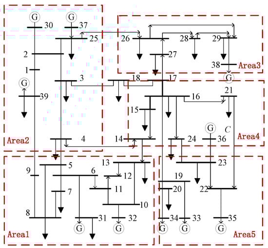
Figure 1. The 10-generator, 39-bus system and its regional partitioning structure.

The parameters of the 10 thermal generating units are listed in Table 1. The wind curtailment penalty coefficient is set to 500 CNY/(MW·h).

Table 1. Parameters of generating units.

Unit Number	Max Output/MW	Min Output/MW	Power Generation Consumption Coefficient
			a/CNY·MW−2	b/CNY·MW−2	c/CNY·MW−2
1	1500	500	0.00048	16.19	1000
2	1200	400	0.00031	17.26	970
3	750	200	0.002	16.6	700
4	800	200	0.00211	16.5	680
5	1000	300	0.00398	19.7	450
6	750	200	0.00712	22.26	370
7	900	250	0.00079	27.74	480
8	950	250	0.00413	25.92	660
9	800	200	0.00222	27.27	665
10	500	100	0.00173	27.79	670

The forecasted load, wind power, and photovoltaic outputs are shown in the figure. The 24 h temperature variation curves for the five areas are presented in Figure 2, and the 24 h load variation curve is shown in Figure 3.

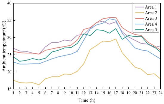
Figure 2. Twenty-four-hour temperature profiles for each area (under normal conditions, peak ambient temperatures are typically reached between 2:00 and 4:00 p.m.; however, in regions with high humidity, this peak may extend until 4:30 or even 5:00 p.m.).

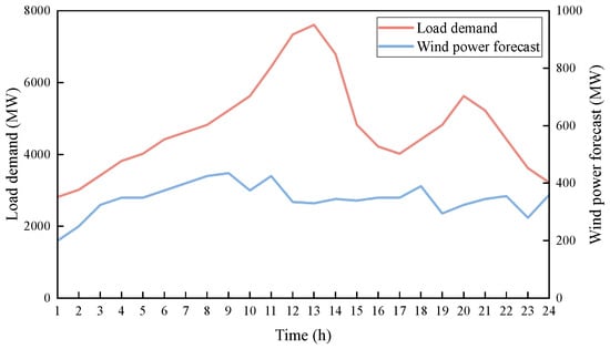
Figure 3. Regional total load and wind power forecast results.

Under the extreme high-temperature typical day scenario, the operation results of different models are shown in the figure. The validation example was conducted over a time period of one day with a time step of 1 h. Figure 4a shows the unit commitment results of the power system under the static thermal stability model, i.e., without considering the transmission line capacity limits and transformer life loss. Figure 4b presents the unit commitment results of the power system, considering the impact of temperature on capacity and transformer life loss.

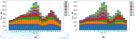
Figure 4. Comparison of unit output results under the extreme high-temperature typical day scenario. (a) Output results of conventional unit commitment method; (b) output results of the TL-TF method.

In the DC power flow dispatch model considering the impact of temperature on the transmission capacity limits of transmission lines, the regional temperature distribution significantly influences generation dispatch decisions and the resilience of the power system. Taking area 2 and area 3 as examples, area 2 (corresponding to Unit 1) maintains relatively low ambient temperatures during the dispatch period, while area 3 (corresponding to Unit 2) experiences sustained high temperatures and even extreme heat events. Under the traditional static thermal rating model, since both Units 1 and 2 have relatively low generation loss coefficients, the system tends to dispatch these two units at higher loads to achieve economic optimality. However, in the model incorporating temperature constraints, the high temperatures in area 3 significantly reduce the transmission capacity limits of its transmission lines, creating bottlenecks that restrict the power export capability of units in this region, thus suppressing the optimal output level of Unit 2. In contrast, units located in lower-temperature regions or those with spare capacity increase their output to compensate for the supply limitations in the high-temperature region. Therefore, this model effectively captures the coupled influence of ambient temperature on power flow paths and unit output allocation, offering higher physical consistency and enhanced operational security. The over-limit conditions of critical interface power flows are shown in Figure 5.

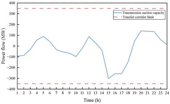
Figure 5. Over-limit conditions of critical interface power flows.

As shown in Figure 5, the transmission capacity of the interfaces did not exceed their limits during the operation day, ensuring the security of critical regional transmission lines.

Regarding transformer life loss, the test case presents a comparative analysis of the average hot-spot temperature of transformers between the proposed TL-TF model and the conventional model, as shown in the figure below:

As shown in Figure 6, the conventional model, which does not consider transformer life loss due to temperature variations, exhibits a rapid increase in transformer hot-spot temperature as the ambient temperature rises. The hot-spot temperature surpasses the maximum allowable limit of 98 °C specified by the IEC guidelines, resulting in accelerated transformer aging. In contrast, the proposed TL-TF model shows only a slight increase in the transformer hot-spot temperature under the influence of ambient temperature, effectively reducing the aging rate and thereby extending the transformer’s service life.

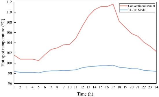
Figure 6. Average transformer hot-spot temperature profiles under the extreme high-temperature typical day scenario.

Based on the above simulation tests, the system costs of the proposed TL-TF model and the conventional model are compared, with the results shown in the table below:

As shown in Table 2, influenced by the transmission capacity limits of lines, the proposed model reduces wind power curtailment by 14.21 MW, thereby providing greater accommodation capacity for wind power and improving curtailment conditions. Meanwhile, the TL-TF model accounts for the impact of ambient temperature on transformer life loss, enabling effective regulation of transformer hot-spot temperatures and reducing transformer loss costs. Consequently, the proposed model decreases the total operating cost by CNY 4000 on the typical day, enhancing the overall economic performance of the system.

Table 2. Comparison of system costs on an extreme high-temperature typical day.

Model	Generation Cost/ (104 CNY)	Start-Up/Shutdown Cost/ (104 CNY)	Wind Curtailment Cost/(104 CNY)	Transformer Loss Cost/ (104 CNY)	Total Cost/ (104 CNY)
TL-TF model	7.01	0.5	0.21	0.04	7.76
Con- Model	7.12	0.67	0.24	0.13	8.16

The case study conducted a sensitivity analysis of the system operation results with respect to the wind curtailment penalty coefficient and the assumed transformer investment cost. In the sensitivity analysis tests, considering the requirements for renewable energy utilization, the wind curtailment penalty coefficient was selected, and different assumptions of transformer investment costs were applied. The corresponding system operation results are presented in Table 3.

Table 3. Impact of wind curtailment penalty and transformer investment cost on system operation.

Wind Curtailment Penalty Coefficient CNY/(MW·h)	Transformer Investment Cost (104 CNY)	Generation Cost/ (104 CNY)	Start-Up/Shutdown Cost/ (104 CNY)	Wind Curtailment Cost/ (104 CNY)	Transformer Loss Cost/ (104 CNY)	Total Cost/ (104 CNY)
100	230	7.15	0.30	0.45	0.03	7.93
300	230	6.99	0.43	0.32	0.04	7.78
500	230	7.01	0.50	0.21	0.04	7.76
1000	230	6.97	0.72	0.13	0.05	7.87
500	190	7.07	0.53	0.21	0.07	7.88
500	260	7.05	0.52	0.20	0.08	7.85

We set the wind curtailment penalty coefficient to 100, 300, 500, and 1000 to observe its impact on the operating results. When the wind curtailment penalty coefficient is low, curtailment is treated as an economically preferable option. The optimization model therefore maintains thermal units at efficient and stable operating levels, resulting in substantial curtailment but limited overall cost due to the low penalty. As the penalty coefficient increases, the system enters a cost-balancing stage, where enhanced wind utilization becomes economically attractive. The model integrates more wind power by committing flexible units for start–stop operations and scheduling thermal units for peak shaving. In this phase, generation costs rise owing to greater flexibility requirements, while curtailment costs decline. With a further increase in the penalty coefficient, the system shifts to a high-cost utilization stage. Near-complete wind absorption is achieved at the expense of frequent cycling of thermal units, leading to sharply higher generation and start-up costs. Overall, the total cost exhibits a U-shaped trend, decreasing initially and then rising as the penalty coefficient increases.

In addition, compared with the standard transformer investment cost, an increase in the investment cost leads to a significant rise in the economic value of unit life loss, thereby increasing the overall life loss cost. When the investment cost decreases, the life loss cost also shows an upward trend. This is mainly attributed to the fact that cost reduction is usually accompanied by structural simplification or lower material grades, which may weaken the thermal stability and aging resistance of the equipment, thereby accelerating the degradation of insulation life.

To thoroughly validate the adaptability and robustness of the proposed TL-TF model under different climatic conditions, a sensitivity analysis is conducted in addition to the original case study. The test settings are as follows: all power system parameters are kept unchanged, while the 24 h ambient temperature curves of all regions in Figure 2 are multiplied by a set of scaling factors $\mathsf{\lambda }$ = (0.9, 1.0, 1.1, 1.2) to simulate varying levels of high-temperature scenarios. For each temperature scenario, both the conventional UC model and the proposed TL-TF model were executed, and the corresponding transformer lifetime loss cost was recorded, as shown in Table 4.

Table 4. Comparison of transformer life loss costs based on different temperature multipliers.

Temperature Multiplier (λ)	Life Loss Cost (Con-Model)/(104 CNY)	Life Loss Cost (TL-TF Model)/(104 CNY)	Cost Reduction
0.9	0.082	0.030	63.4%
1.0	0.130	0.040	69.2%
1.1	0.189	0.051	73.0%
1.2	0.285	0.680	76.1%

With the increase in ambient temperature, the transformer life loss cost rises significantly in both models, confirming that the cost function of transformer life loss is highly sensitive to temperature-driven factors. More importantly, under all temperature scenarios, the TL-TF model consistently achieves lower life loss costs compared with the conventional model. Furthermore, as the temperature scaling factor $\mathsf{\lambda }$ increases, the cost reduction ratio obtained by the TL-TF model becomes larger. This indicates that by optimizing the scheduling of generation outputs, power flows, and transformer loading, the TL-TF model can more effectively cope with extreme high-temperature conditions. The sensitivity analysis therefore demonstrates that the proposed TL-TF-based optimal scheduling approach exhibits good adaptability in the face of varying levels of temperature rise.

6. Conclusions

This paper addresses the critical challenges of deteriorating transmission line thermal stability and accelerated transformer aging in power systems under extreme climate conditions by proposing an optimized dispatch method that incorporates the dynamic thermal stability of transmission lines and transformer aging losses. The main research findings are summarized as follows:

• The proposed dynamic ampacity calculation model, based on thermal equilibrium theory, enables real-time transmission capacity assessment by accounting for the impacts of ambient temperature, wind speed, and solar radiation on the conductor temperature rise. The simulation results demonstrate a 12% improvement in transmission capacity utilization in high-temperature regions compared to conventional static line rating methods, effectively alleviating transmission bottlenecks caused by extreme heat.
• By considering the combined effects of ambient temperature and the load ratio on transformer hot-spot temperature and employing linear damage accumulation theory, the developed transformer aging cost function achieves a 69% reduction in transformer aging costs, significantly extending transformer service life.
• The proposed UC model simultaneously optimizes generation costs, transformer aging losses, and wind curtailment penalties. Case studies show that compared to conventional methods, this approach reduces wind curtailment by 12.5% and decreases total operating costs by 4.9%, substantially enhancing both the economic efficiency and operational security of power dispatch under extreme high-temperature conditions.

References

- Qin, Z.; Chen, X.; Hou, Y.; Liu, H.; Yang, Y. Coordination of Preventive, Emergency and Restorative Dispatch in Extreme Weather Events. IEEE Trans. Power Syst. 2022, 37, 2624–2638. [Google Scholar] [CrossRef]
- Trakas, D.N.; Hatziargyriou, N.D. Strengthening Transmission System Resilience Against Extreme Weather Events by Undergrounding Selected Lines. IEEE Trans. Power Syst. 2022, 37, 2808–2820. [Google Scholar] [CrossRef]
- Zhou, J.; Liu, J.; Jiang, Z.; Gong, H.; Fan, X.; Lin, Y.; Wang, Q.; Gao, B. Effect of Testing Temperature Gradients on Dielectric Polarization Parameters of Transformer Oil-Paper Insulation. IEEE Trans. Dielectr. Electr. Insul. 2025, 32, 1460–1467. [Google Scholar] [CrossRef]
- Ilunga, K.G.; Swanson, A.G.; Ijumba, N.M.; Stephen, R. Experimental Investigation of the Effect of Conductor Temperature on Corona Performance in Overhead Transmission Lines. IEEE Access 2024, 12, 122114–122125. [Google Scholar] [CrossRef]
- Albizu, I.; Fernandez, E.; Alberdi, R.; Bedialauneta, M.T.; Mazon, A.J. Adaptive Static Line Rating for Systems with HTLS Conductors. IEEE Trans. Power Deliv. 2018, 33, 2849–2855. [Google Scholar] [CrossRef]
- González-Cagigal, M.; Rosendo-Macías, J.A.; Bachiller-Soler, A.; Del-Pino-López, J.C. Reliability Assessment of Dynamic Line Rating Methods Based on Conductor Temperature Estimation. Electr. Power Syst. Res. 2024, 233, 110449. [Google Scholar] [CrossRef]
- Bhattarai, B.P.; Gentle, J.P.; McJunkin, T.; Hill, P.J.; Myers, K.S.; Abboud, A.W.; Hengst, D. Improvement of Transmission Line Ampacity Utilization by Weather-Based Dynamic Line Rating. IEEE Trans. Power Deliv. 2018, 33, 1853–1863. [Google Scholar] [CrossRef]
- Gezegin, C.; Ozgonenel, O.; Dirik, H. A Monitoring Method for Average Winding and Hot-Spot Temperatures of Single-Phase, Oil-Immersed Transformers. IEEE Trans. Power Deliv. 2021, 36, 3196–3203. [Google Scholar] [CrossRef]
- Wang, X.; Li, Y.; Yu, Z.; Miao, Y.; Li, P.; Xu, Z. Analysis Method of Transformer Fatigue Life and Damage Under Multiple Short-Circuit Conditions. IEEE Trans. Appl. Supercond. 2024, 34, 1–4. [Google Scholar] [CrossRef]
- Paramane, S.B.; Joshi, K.; Van der Veken, W.; Sharma, A. CFD Study on Thermal Performance of Radiators in a Power Transformer: Effect of Blowing Direction and Offset of Fans. IEEE Trans. Power Deliv. 2014, 29, 2596–2604. [Google Scholar] [CrossRef]
- Fathi, S.; Ghahremani, A.; Shafii, M.B.; Sadr, M.; Salehzehi, A. Improving Transformer Cooling Performance Through Advanced Heat Pipes Integration. Appl. Therm. Eng. 2025, 267, 125775. [Google Scholar] [CrossRef]
- Zhang, Y.; Wei, X.; Fan, X.; Wang, K.; Zhuo, R.; Zhang, W.; Liang, S.; Hao, J.; Liu, J. A Prediction Model of Hot Spot Temperature for Split-Windings Traction Transformer Considering the Load Characteristics. IEEE Access 2021, 9, 22605–22615. [Google Scholar] [CrossRef]
- Bagheri, A.; Mobayen, S.; Osali, N. An MIQCP-based multi-objective optimal operation strategy for renewables-integrated smart distribution systems considering transformer loss of life and environmental emissions. Electr. Power Syst. Res. 2025, 239, 111252. [Google Scholar] [CrossRef]
- Hosseinkhanloo, M.; Kalantari, N.T.; Behjat, V.; Ravadanegh, S.N. Optimal exploitation of power transformer fleet considering loss of life and economic evaluation based on failure probability. Electr. Power Syst. Res. 2022, 213, 108801. [Google Scholar] [CrossRef]
- Shaker, H.; Fotuhi-Firuzabad, M.; Aminifar, F. Fuzzy Dynamic Thermal Rating of Transmission Lines. IEEE Trans. Power Deliv. 2012, 27, 1885–1892. [Google Scholar] [CrossRef]
- Wang, M.; Yang, M.; Wang, J.; Wang, M.; Han, X. Contingency Analysis Considering the Transient Thermal Behavior of Overhead Transmission Lines. IEEE Trans. Power Syst. 2018, 33, 4982–4993. [Google Scholar] [CrossRef]
- Davidzon, M.I. Newton’s law of cooling and its interpretation. Int. J. Heat Mass Transf. 2012, 55, 5397–5402. [Google Scholar] [CrossRef]
- Ngoko, B.; Sugihara, H.; Funaki, T. Validation of a Simplified Model for Estimating Overhead Conductor Temperatures under Dynamic Line Ratings—Comparison with the CIGRE Model. IEEJ Trans. Power Energy 2018, 138, 284–296. [Google Scholar] [CrossRef]
- Frank, S.; Sexauer, J.; Mohagheghi, S. Temperature-Dependent Power Flow. IEEE Trans. Power Syst. 2013, 28, 4007–4018. [Google Scholar] [CrossRef]
- Luo, C.; Li, Z.; Yang, B.; Zhao, Z.; Li, C. Hot-Spot Dynamic Temperature Rise of Oil-Immersed Transformer Through FBG-Based Multipoint Sensing System. IEEE Sensors J. 2025, 25, 25743–25753. [Google Scholar] [CrossRef]
- Hashmi, M.; Lehtonen, M.; Hänninen, S. Effect of Climate Change on Transformers Loading Conditions in the Future Smart Grid Environment. Open J. Appl. Sci. 2013, 3, 24–29. [Google Scholar] [CrossRef]
- Li, Y.; Zhang, C.; Li, J.; Song, W.; Qi, Z.; Wu, Y.; Wu, X. MCoR-Miner: Maximal Co-Occurrence Nonoverlapping Sequential Rule Mining. IEEE Trans. Knowl. Data Eng. 2023, 35, 9531–9546. [Google Scholar] [CrossRef]
- Djamali, M.; Tenbohlen, S. Malfunction Detection of the Cooling System in Air-Forced Power Transformers Using Online Thermal Monitoring. IEEE Trans. Power Deliv. 2017, 32, 1058–1067. [Google Scholar] [CrossRef]
- GB/T 38969-2020; Guide on Technology for Power System. Standards Press of China: Beijing, China, 2020.
- Zhou, H.; Ju, P.; Xue, Y.; Zhu, J. Probabilistic Equivalent Model of DFIG-based Wind Farms and Its Application in Stability Analysis. J. Mod. Power Syst. Clean Energy 2016, 4, 248–255. [Google Scholar] [CrossRef]
Disclaimer/Publisher’s Note: The statements, opinions and data contained in all publications are solely those of the individual author(s) and contributor(s) and not of MDPI and/or the editor(s). MDPI and/or the editor(s) disclaim responsibility for any injury to people or property resulting from any ideas, methods, instructions or products referred to in the content. |
© 2025 by the authors. Licensee MDPI, Basel, Switzerland. This article is an open access article distributed under the terms and conditions of the Creative Commons Attribution (CC BY) license (https://creativecommons.org/licenses/by/4.0/).