A Fault-Tolerant Proportional-Integral-Derivative Load Frequency Control for Power Systems Operating Under a Random Event-Triggered Scheme

Abstract

This paper proposes a novel fault-tolerant proportional-integral-derivative (PID) control method for load frequency control (LFC) in power systems, addressing performance degradation caused by controller failures. Firstly, a unified fault model for actuators is established, and a fault-tolerant PID control strategy is developed. Subsequently, a random event-triggering scheme (RETS) is introduced, utilizing a Poisson random probability sampling period to minimize redundant network communication resource usage. The stability of the closed-loop system is rigorously verified through Lyapunov function analysis. Finally, the effectiveness of the proposed control method and the superiority of RETS are demonstrated via an illustrative case study on an isolated power system.

1. Introduction

The power grid is a typical intricate system for controlling networks, where every component generates power, consumes power, and distributes electricity to connected areas in a timely manner to uphold the equilibrium of power demand and supply [1,2]. Preserving stable functionality requires maintaining the local frequency difference and the power transmission through tie-lines at a set standard value [3,4]. Therefore, the main emphasis in power system control is to mitigate deviations in frequency and tie-line power flow from their anticipated levels, while accounting for the repercussions of load disturbances [5].

An effective approach has been implemented for power system load frequency control to accomplish task [6]. In traditional approach, frequency stableness for every area is typically achieved whit a single control center [7], this architecture is referred to as centralized control architecture. Nevertheless, the conventional centralized control system has a significant drawback, if the centralized controller fails, it can lead to the entire global system being left in an unregulated state [8,9]; moreover, this drawback is especially detrimental to the frequency stableness of bulk power systems. On the flip side, the rising penetration of abundant, yet variable, sustainable energy sources results in power imbalances within power systems [10]. To address the issue of system failure stemming from a centralized control framework, researchers introduced a distributed power system control architecture [11,12]. This approach has proven effective in maintaining frequency stability in large power systems. Furthermore, the growing prevalence of unpredictable renewable energy sources results in power imbalances within the system, rendering traditional centralized control impractical due to the extensive inertia of synchronous generator sets. Consequently, the distributed control architecture offers a viable solution for mitigating the risk of a single controller failure leading to system collapse. Numerous effective control techniques have been proposed in recent decades [13]. While an output feedback controller with counterfeit attack signals has been developed, it relies on a centralized framework. Subsequently, decentralized proportional integration (PI) control methodologies leveraging local feedback error signals, known as area control errors (ACE), have gained widespread acceptance [2,14,15]. Notably, there is limited research on distributed proportional integral derivative (PID) controllers within the current LFC power system domain. Furthermore, the power system represents a sophisticated cyber-physical structure comprising multiple electrical and communication apparatus [16,17]. In such a sprawling and intricate system, the breakdown of the execution mechanism is foreseeable [18,19]. Enhancing the fault tolerance of the controller presents a separate obstacle; hence, a strategy for fault tolerant PID control is introduced in the study.

Digital devices are commonly utilized in power systems for gathering and transmitting control data [20]. Thus far, the predominant techniques for sampling control data encompass periodic, aperiodic within bounded intervals, and stochastic sampling [21]. Currently, control data sampling techniques consist of periodic sampling, bounded interval aperiodic sampling, and random sampling. For instance, the wind power system described in [22] implements aperiodic sampling for control data and sets up an exponential frequency stability criterion to ensure a rapid frequency response. Nevertheless, various physical limitations may result in random sampling intervals, such as deteriorating efficiency of data transmission devices and occasional sensor malfunctions. As a result, the actual sampling intervals are influenced by noise and deviate from the ideal intervals with a specific probability distribution [23]. With the advancement of wide-area measurement technology, wireless communication platforms can be used to transmit sampled data. Due to limited communication resources in wireless networks, preventing redundant occupation of communication channels has become a major research focus. Event-triggered communication schemes serve as an effective method to enhance network communication bandwidth utilization. A crucial aspect of event-triggering schemes (ETS) involves developing suitable trigger threshold conditions for determining when to transmit a decentralized control signal. Furthermore, digitally sampled information is only broadcasted when predefined trigger conditions are breached, thereby striking a balance between frequency stability and resource conservation.

Several works in the literature [24,25,26] present various studies designing event-triggered systems (ETS) for effective frequency regulation. Lu et al. [24] proposed a universally applicable periodic event-triggering scheme (PETS) tailored for networked control systems. Subsequently, an accommodation for event-triggered system was developed, building upon PETS concept, which could dynamically adjust trigger threshold conditions based on system state fluctuations [27]. Another recent study [26] presented a dynamic memory ETS that effectively utilizes past data to establish trigger threshold conditions. Different ETS design approaches include memory ETS [17], dynamic ETS [28], and ETS tailored for specific performance criteria [29], and SETS [14]. This paper proposes a novel method involving randomly sampled data patterns based on Poisson random probability. The main contributions of this paper can be summarized as follows:

(1)

Utilizing the unified model and actuator fault model for isolated power systems, a PID controller with fault tolerance is developed for power systems.

(2)

Unlike conventional PETSs [30], a series of randomly updated sampling intervals based on Poisson stochastic processes is introduced to depict communication patterns, leading to a reduction in the unnecessary use of communication resources.

(3)

By formulating suitable Lyapunov–Krasovskii functionals (LKFs), we establish a stability criterion for standalone power systems with $H_{\infty }$ performance. Following this, we conduct a comparative analysis to validate the efficacy of the proposed control strategy and demonstrate the benefits of RETS.

Notation: N denotes the natural numbers set and $N^{+}$ denotes the positive integers set. ${\mathbb{R}}^n$ and ${\mathbb{R}}^{n\times m}$ represent the Euclidean space of n dimensions and collection of $n\times m$ real matrices. $Q^{⊺}$ and $Q^{-1}$ indicate the transpose and inverse of the matrix Q. A matrix Q is considered to be symmetric and positive (semi-positive) when $Q>0$ ($Q\ge 0$).

2. Preliminaries

Initially, Section 2.1 meticulously elucidates the intricate dynamics of a solitary power system domain. Then, a PID control tactic with fault tolerance is formulated in a distributed manner, taking into account actuator faults in Section 2.2. Ultimately, a new RETS is devised in Section 2.3 to reduce the occupancy of network bandwidth.

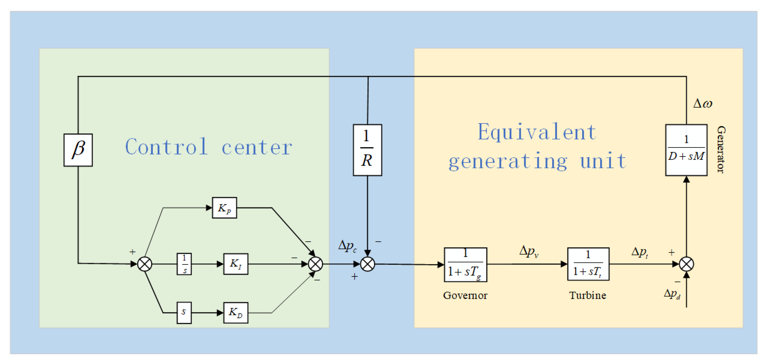
2.1. Power System Load Frequency Control Model

The following widely accepted standard assumptions are made regarding the system [31]:

(a)

The size of the bus voltage $\left|V\right|$ remains constant;

(b)

The power network is considered to be without losses.

The dynamical model shown in Figure 1 is established for the area as follows:

It is given that the dynamic behavior of the system can be described as follows:

$$\begin{array}{cc}\hfill \dot{\theta }\left(t\right)& =\omega \left(t\right),\hfill \\ \hfill M\dot{\omega }\left(t\right)& =p_t\left(t\right)-D\omega \left(t\right)-p_d\left(t\right),\hfill \\ \hfill T_t{\dot{p}}_t\left(t\right)& =-p_t\left(t\right)+p_v\left(t\right),\hfill \\ \hfill T_g{\dot{p}}_g\left(t\right)& ={\displaystyle \frac{1}{R}}\omega \left(t\right)-p_g\left(t\right)+p_c\left(t\right).\hfill \end{array}$$

(1)

Define $ACE\left(t\right)=\beta \Delta \omega \left(t\right)$, and let $u\left(t\right)=\Delta p_c\left(t\right),\phi \left(t\right)=\Delta p_d\left(t\right)$,

$$x\left(t\right)=\mathrm{col}\left(\Delta \omega \left(t\right),\Delta p_t\left(t\right),\Delta p_{\mathrm{g}}\left(t\right)\right),$$

$$y\left(t\right)=ACE\left(t\right).$$

$$x\left(t\right)=\mathrm{col}\left(\Delta \omega \left(t\right),\Delta p_t\left(t\right),\Delta p_{\mathrm{g}}\left(t\right)\right),$$

$$y\left(t\right)=ACE\left(t\right).$$

Then, the system is reformulated as

$$\left\{\begin{array}{c}\begin{array}{cc}\hfill \dot{x}\left(t\right)& =Ax\left(t\right)+Bu\left(t\right)+F\phi \left(t\right),\hfill \\ \hfill y\left(t\right)& =Cx\left(t\right).\hfill \end{array}\hfill \end{array}\right.$$

(2)

where

$$A=\left[\begin{array}{ccc}-{\displaystyle \frac{D}{M}}& {\displaystyle \frac{1}{M}}& 0\\ 0& -{\displaystyle \frac{1}{Tt}}& {\displaystyle \frac{1}{Tt}}\\ -{\displaystyle \frac{1}{RTg}}& 0& -{\displaystyle \frac{1}{Tg}}\end{array}\right],B=\left[\begin{array}{c}0\\ 0\\ {\displaystyle \frac{1}{Tg}}\end{array}\right],F=\left[\begin{array}{c}-{\displaystyle \frac{1}{M}}\\ 0\\ 0\end{array}\right],C={\left[\begin{array}{c}\beta \\ 0\\ 0\end{array}\right]}^T$$

The notations of the system parameters in Equations (1) and (2) are summarized in

Table 1. Notations.

D	Generator damping coefficient	$p_t\left(t\right)$	Generator output deviation
M	Generator inertia moment	$p_v\left(t\right)$	Generator valve position deviation
$T_t$	Turbine time constant	$p_c\left(t\right)$	Control command deviation
$T_g$	Governor time constant	$p_d\left(t\right)$	Load deviation
R	Speed drop factor	$\omega \left(t\right)$	Frequency
$\beta$	Frequency bias coefficient	$ACE\left(t\right)$	Area control error signal

.

2.2. A Fault-Tolerant PID Control

• Actuator fault model

The actuator fault model used in [14] is adopted. For the actuator, $u\left(t\right)$ and $u^g\left(t\right)$ represent the input and the output, separately. It fulfills the requirement

$$\begin{array}{c}\hfill u^g\left(t\right)=\psi u\left(t\right)\end{array}$$

(3)

The value of $\psi$, an unknown fault coefficient, must satisfy the condition $0\le \psi \le 1$. Actuator faults can be categorized into three scenarios:

• Fault-free: $\psi =1$;
• Fault of reduced effectiveness: $0<\psi <1$;
• Outage fault: $\psi =0$.

2.

A fault-tolerant PID control tactic.

In this study, $u\left(t\right)$ is designed as the subsequent PID control input:

$$\begin{array}{c}\hfill u\left(t\right)=-(K_{P}ACE\left(t\right)+K_I\int ACE\left(t\right)+K_D{\displaystyle \frac{dACE\left(t\right)}{dt}})\end{array}$$

(4)

$u\left(t\right)$ is controller output. The parameter $K_P$ represents the proportional gain of the controller, $K_I$ denotes integral gain, and $K_D$ signifies differential gain.

By incorporating actuator faults into consideration, adjustments can be made to the PID control strategy as

$$\begin{array}{c}\hfill u^g\left(t\right)=-\psi (K_{P}ACE\left(t\right)+K_I\int ACE\left(t\right)+K_D{\displaystyle \frac{dACE\left(t\right)}{dt}})\end{array}$$

(5)

The system virtual state variables and output variables are defined as below:

$$\left\{\begin{array}{c}\begin{array}{cc}\hfill \overline{\mathit{x}}\left(t\right)& ={\left[\begin{array}{cc}{\mathit{x}}^{\mathrm{T}}\left(t\right)& \int {\mathit{y}}^{\mathrm{T}}\left(t\right)\mathrm{d}t\end{array}\right]}^{\mathrm{T}}\hfill \\ \hfill \overline{\mathit{y}}\left(t\right)& ={\left[\begin{array}{ccc}{\mathit{y}}^{\mathrm{T}}\left(t\right)& \int {\mathit{y}}^{\mathrm{T}}\left(t\right)\mathrm{d}t& {\displaystyle \frac{\mathrm{d}}{\mathrm{d}t}}{\mathit{y}}^{\mathrm{T}}\left(t\right)\end{array}\right]}^{\mathrm{T}}\hfill \end{array}\hfill \end{array}\right.$$

(6)

Contemplate the subsequent system (2) with the controller

$$\begin{array}{c}\hfill \left\{\begin{array}{c}\dot{x}\left(t\right)=\overline{A}x\left(t\right)-\overline{B}u\left(t\right)+\overline{F}\phi \left(t\right)\hfill \\ \overline{y}\left(t\right)=\overline{C}x\left(t\right)+{\overline{D}}_{\omega }\phi \left(t\right)\hfill \\ u\left(t\right)=-K\psi \overline{y}\left(t\right)\hfill \end{array}\right.\end{array}$$

(7)

$\overline{A}=\left(\begin{array}{cccc}-{\displaystyle \frac{D}{M}}& {\displaystyle \frac{1}{M}}& 0& 0\\ 0& -{\displaystyle \frac{1}{Tt}}& {\displaystyle \frac{1}{Tt}}& 0\\ -{\displaystyle \frac{1}{RTg}}& 0& -{\displaystyle \frac{1}{Tg}}& 0\\ \beta & 0& 0& 0\end{array}\right)$, $\overline{B}=\left[\begin{array}{c}0\\ 0\\ {\displaystyle \frac{1}{Tg}}\\ 0\end{array}\right]$, $\overline{F}=\left[\begin{array}{c}-{\displaystyle \frac{1}{M}}\\ 0\\ 0\\ 0\end{array}\right]$, $\overline{C}=\left[\begin{array}{cccc}\beta & 0& 0& 0\\ 0& 0& 0& 1\\ -{\displaystyle \frac{D\beta }{M}}& {\displaystyle \frac{\beta }{M}}& 0& 0\end{array}\right]$, $\overline{D}\omega =\left[\begin{array}{c}-{\displaystyle \frac{\beta }{M}}\\ 0\\ 0\end{array}\right]$, $K=\left[\begin{array}{ccc}{K}_P& K_I& K_D\end{array}\right]$.

Then, system (7) is rewritten as

$$\left\{\begin{array}{c}\begin{array}{cc}\hfill \dot{\overline{x}}\left(t\right)& =\overline{A}\overline{x}\left(t\right)-\overline{B}\psi K\overline{C}\overline{x}\left(t\right)+(\overline{F}-\overline{B}\psi K\overline{D}\omega \phi \left(t\right))\hfill \\ \hfill \overline{y}\left(t\right)& =\overline{C}\overline{x}\left(t\right)+\overline{D}\omega \phi \left(t\right)\hfill \end{array}\hfill \end{array}\right.$$

(8)

2.3. Poisson Random Events to Trigger Communication Scheme

At the section, an event-triggered scheme derived from the Poisson random probability sample pattern is introduced. Initially, revisit the PETS proposed in [24]:

$$t_{k+1}h=t_{k}h+min\{mh\mid \tilde{f}(x\left(t_{k}h\right),\tilde{e}\left(mh\right),\tilde{\mu })>0\}$$

(9)

where h denotes the sampling period, $t_{k}h$ represents the most recent transmission instant, and ${\left\{t_k\right\}}_{k=0}^{+\infty }$ is an increasing sequence with $t_k\in \mathbb{N}$, $\tilde{\mu }>0$ characterizes the event-triggering mechanism in the periodic sampling mode, $\tilde{e}\left(mh\right)=x(t_{k}h+mh)-x\left(t_{k}h\right)$ is the state error, and $\tilde{F}(x\left(t_{k}h\right),\tilde{e}\left(mh\right),\tilde{\mu })={\tilde{e}}^{\mathrm{T}}\left(mh\right)\tilde{\Omega }\tilde{e}\left(mh\right)-\tilde{\mu }{x}^{\mathrm{T}}\left(t_{k}h\right)\tilde{\Omega }x\left(t_{k}h\right)$. The sensor periodically captures system states with a period of h. If the most recent transmission status $x\left(t_{k}h\right)$ and the error satisfy the condition for the threshold for event-triggered triggering in (9), then the subsequent transmission moment $\tilde{e}\left(mh\right)$ should meet the event-triggered threshold in (9) and subsequently determine the next transmission instant $t_{k+1}$.

Drawing inspiration from PETS, a Random Event-Triggered Scheme (RETS) is designed. First, a random sampling sequence is defined as ${\left\{m_{l}h\right\}}_{l=0}^{\infty }$, where $h\in {\mathbb{N}}_{+}$ and $m_{l+1}=m_l+m_l^s$, with initial conditions $m_0=0$, $m_0^s=0$. Here, $m_l^s\in \{1,\dots ,\overline{m}\}$ is a random sampling coefficient active during the interval $[m_{l}h,m_{l+1}h)$, and $\overline{m}\in {\mathbb{N}}_{+}$ denotes the upper bound of $m_l^s$.

The probability distribution of the random variable $m_l^s$ is given by the function:

$$f\left(x\right)={\displaystyle \frac{e^{-\lambda x}{\left(\lambda x\right)}^n}{n!}},x=1,2,\dots ,\overline{m}-1,$$

where $\lambda \in [0,1)$ is a tunable parameter, and $n=1$.

There is a close relationship between Poisson random distribution and event-triggering; especially when describing the frequency or time interval of random events, we can understand the randomness and regularity between events, which is helpful to optimize resource allocation and alleviate redundancy.

Accordingly, the transmission instants can be determined using the RETS:

$$\begin{array}{c}\hfill t_{k+1}h=t_{k}h+\underset{m_l\in {\mathbb{N}}_{+}}{min}\{m_{l}h{|}_F(x\left(t_{k}h\right),e\left(m_l^{s}h\right),\mu )>0\},\end{array}$$

(10)

where $F(x\left(t_{k}h\right),e\left(m_l^{\mathrm{s}}h\right),\mu )=e^{\mathrm{T}}\left(m_l^{\mathrm{s}}h\right)\Omega e\left(m_l^{\mathrm{s}}h\right)-\mu x^{\mathrm{T}}\left(t_{k}h\right)\Omega x\left(t_{k}h\right),$ $e\left(m_l^{\mathrm{s}}h\right)=x(t_{k}h+m_l^{\mathrm{s}}h)-x\left(t_{k}h\right),\mu >0$, and $\Omega >0$ are the design tasks that involve determining the parameter for event triggering and the weighting matrix for event triggering, respectively, as shown in Figure 2.

Considering the stochastic nature of communication triggered by events with the presence of actuator faults, system (8) undergoes rewriting as

$$\begin{array}{c}\hfill \left\{\begin{array}{c}\dot{\overline{x}}\left(t\right)=\overline{A}x\left(t\right)-\overline{B}\psi K\overline{C}\overline{x}\left(tkh\right)+(\overline{F}-\overline{B}K\psi {\overline{D}}_{\omega })\phi \left(t\right)\hfill \\ \overline{y}\left(t\right)=\overline{C}\overline{x}\left(t\right)+\overline{D}\omega \phi \left(t\right)\hfill \end{array}\right.\end{array}$$

(11)

Define $\eta \left(t\right)=t-(t_k+m_l^s)h$ and $0<\eta \left(t\right)<\overline{\eta }$. Derived from the explanations of $\eta \left(t\right)$ with $e\left(m_l^{s}h\right)$, system (11) can be transformed as

$$\begin{array}{c}\hfill \left\{\begin{array}{c}\dot{\overline{x}}\left(t\right)=\overline{A}\overline{x}\left(t\right)-\overline{B}\psi KC\overline{x}(t-\eta \left(t\right))+\overline{B}\psi K\overline{C}e\left(m_l^{s}h\right)+(\overline{F}-\overline{B}K\psi \overline{D}\omega )\phi \left(t\right)\hfill \\ \overline{y}\left(t\right)=\overline{C}\overline{x}\left(t\right)+\overline{D}\omega \phi \left(t\right).\hfill \end{array}\right.\end{array}$$

(12)

Remark 1. 

RETS (10) is designed based on a random sampling method, where each sampling interval $m_l^{s}h$ is randomly generated. When $m_l^{s}h=1$, RETS reduces to PETS (9). In this case, the event-triggering condition is always satisfied, causing RETS (10) to degenerate into a periodic sampling mode.

3. Primary Outcomes

3.1. Analysis of Controllability

Theorem 1. 

In the presence of any consistent load disruption, $\phi \left(t\right)=\overline{\phi }$. The system featuring PID control input is said to be steerable, meaning it is possible to drive the system output to any desired trajectory using suitable control input over time. Let $\mathrm{T}=\left[\begin{array}{cc}\overline{A}& -\overline{B}K\\ -\overline{C}& I\end{array}\right]$.

Proof. 

Through the introduction of an additional parameter, $h\left(t\right)=\widehat{y}\left(t\right)-\overline{y}\left(t\right)$, $\widehat{y}\left(t\right)$ represents the output reference value of $\overline{y}\left(t\right)$. Control objectives are achieved as ${lim}_{t\to \infty }h\left(t\right)=0$.

$$\begin{array}{c}\hfill \left[\begin{array}{c}\dot{\overline{x}}\left(t\right)\\ h\left(t\right)\end{array}\right]=\left[\begin{array}{ccc}\overline{A}-\overline{B}K\overline{C}& & 0\\ -\overline{C}& & 0\end{array}\right]\left[\begin{array}{c}\overline{x}\left(t\right)\\ h\left(t\right)\end{array}\right]+\left[\begin{array}{c}\overline{F}-\overline{B}K\overline{D}\omega \\ -\overline{D}\omega \end{array}\right]\overline{\phi }+\left[\begin{array}{c}0\\ I\end{array}\right]\widehat{y}\left(t\right).\end{array}$$

(13)

$h\left(t\right)=0$ suggests that

$$\begin{array}{c}\hfill \overline{C}\overline{x}\left(t\right)=\widehat{y}\left(t\right)-\overline{D}\omega \overline{\phi },\end{array}$$

(14)

let $\dot{\overline{x}}\left(t\right)=0$ that

$$\begin{array}{c}\hfill \overline{A}\overline{x}\left(t\right)-\overline{B}K\widehat{y}\left(t\right)=-\overline{F}\overline{\phi }.\end{array}$$

(15)

Let ${\xi }_1\left(t\right)={[{\overline{x}}^{\mathrm{T}}\left(t\right),{\widehat{y}}^{\mathrm{T}}\left(t\right)]}^{\mathrm{T}}$ and ${\xi }_2={[0,-{\left(F\overline{\phi }\right)}^{\mathrm{T}}]}^{\mathrm{T}}$. Finding a solution for $\overline{\mathit{\phi }}$ is thus equivalent to solving the linear system $\mathrm{T}{\xi }_1\left(t\right)={\xi }_2\left(t\right)$. Therefore, system (12) admits a solution (i.e., has a balance) if and only if the matrix $\mathrm{T}$ is of full rank. □

3.2. Stability Assessment

Theorem 2. 

If matrices exist $P>0, Q>0, S>0, \Omega >0$, the system achieves asymptotic stability with $\overline{\eta }>0, \mu >0, \gamma >0$ and any matrices $Y_{11},Y_{12},Y_{22},Z_{11},Z_{12},Z_{22},W$ and U and with

$$\begin{array}{c}\hfill {\left.\Xi \left(\eta \right(t\left)\right)\right|}_{\eta \left(t\right)=0}<0,{\left.\Xi \left(\eta \right(t\left)\right)\right|}_{\eta \left(t\right)=\overline{\eta }}<0,\end{array}$$

(16)

$$\begin{array}{c}\hfill \left[\begin{array}{ccc}{Y}_{11}& & Y_{12}\\ Y_{12}^{\mathrm{T}}& & Y_{22}\end{array}\right]\ge 0,\left[\begin{array}{ccc}{Z}_{11}& & Z_{12}\\ Z_{12}^{\mathrm{T}}& & Z_{22}\end{array}\right]\ge 0,\end{array}$$

(17)

$$\begin{array}{c}\hfill Y_{22}-S\le 0,Z_{22}-S\le 0\end{array}$$

(18)

with $\Xi \left(\eta \left(t\right)\right)={\Xi }_1+\eta \left(t\right)Y_{11}+(\overline{\eta }-\eta \left(t\right))Z_{11},$

${\Xi }_1=2e_{4}P{e}_1^T+e_{1}Q{e}_1^T-e_{3}Q{e}_3^T+\overline{\eta }{fe}_{4}S{e}_4^T-{\gamma }^2{e}_6{e}_6^T+e_1{C}^{T}C{e}_1^T+Y_{12}{(e_1-e_2)}^T$$+(e_1-e_2)Y_{12}^T+Z_{12}{(e_2-e_3)}^T$$+(e_2-e_3)Z_{12}^T+W(e_s^T-e_4^T)+(e_s-e_4)W^T$$+\mu (e_2-e_5)\Omega {(e_2-e_5)}^T-e_5\Omega e_5^T,$

$e_s^T=\overline{A}{e}_1^T-\overline{B}\Psi K\overline{C}{e}_2^T+\overline{B}\Psi K\overline{C}{e}_5^T+(\overline{F}-\overline{B}\Psi K\overline{D}\omega )e_6^T$, $e_i=\mathrm{col}(0_{(i-1)n\times n},I_n,0_{(6-i)n\times n})$, $i=1,\dots ,6$.

Proof. 

Create subsequent LKFs:

$$\begin{array}{c}\hfill V\left(t\right)={\overline{x}}^{\mathrm{T}}\left(t\right)P\overline{x}\left(t\right)+{\int }_{t-\overline{\eta }}^t{\overline{x}}^{\mathrm{T}}\left(\rho \right)Q\overline{x}\left(\rho \right)d\rho +{\int }_{-\overline{\eta }}^0{\int }_{t+\rho }^t{\dot{\overline{x}}}^{\mathrm{T}}\left(s\right)S\dot{\overline{x}}\left(s\right)dsd\rho \end{array}$$

(19)

One can calculate the rate of change of $V\left(t\right)$ along the trajectory of system (12) as follows:

$$\begin{array}{c}\hfill \dot{V}\left(t\right)={\zeta }^{\mathrm{T}}\left(t\right)(2e_{4}P{e}_1^{\mathrm{T}}+e_{1}Q{e}_1^{\mathrm{T}}-e_{3}Q{e}_3^{\mathrm{T}}+\overline{\eta }{e}_{4}S{e}_4^{\mathrm{T}})\zeta \left(t\right)-{\int }_{t-\overline{\eta }}^t{\dot{\overline{x}}}^T\left(\rho \right)S\dot{\overline{x}}\left(\rho \right)d\rho \end{array}$$

(20)

with $\zeta \left(t\right)\triangleq col(\overline{x}\left(t\right),\overline{x}(t-\eta \left(t\right)),\overline{x}(t-\overline{\eta }),\dot{\overline{x}}\left(t\right),e\left(m_l^{s}h\right),\phi \left(t\right)).$

Utilizing the integral inequality lemma [32], subsequent inequations are valid of $\left[\begin{array}{ccc}{Y}_{11}& & Y_{12}\\ Y_{12}^{\mathrm{T}}& & Y_{22}\end{array}\right]\ge 0,\left[\begin{array}{ccc}{Z}_{11}& & Z_{12}\\ Z_{12}^{\mathrm{T}}& & Z_{22}\end{array}\right]\ge 0$:

$$\begin{array}{c}0\le {\int }_{t-\eta \left(t\right)}^t{\left[\begin{array}{c}\zeta \left(t\right)\\ \dot{\overline{x}}\left(\rho \right)\end{array}\right]}^{\mathrm{T}}\left[\begin{array}{cc}{Y}_{11}& Y_{12}\\ Y_{12}^{\mathrm{T}}& Y_{22}\end{array}\right]\left[\begin{array}{c}\zeta \left(t\right)\\ \dot{\overline{x}}\left(\rho \right)\end{array}\right]d\rho ={\zeta }^{\mathrm{T}}\left(t\right)\left(Y_{12}{(e_1-e_2)}^{\mathrm{T}}+(e_1-e_2)Y_{12}^{\mathrm{T}}+\eta \left(t\right)Y_{11}\right)\zeta \left(t\right)\hfill \\ +{\int }_{t-\eta \left(t\right)}^t{\dot{\overline{x}}}^{\mathrm{T}}\left(\rho \right)Y_{22}\dot{\overline{x}}\left(\rho \right)d\rho \hfill \end{array}$$

(21)

$$\begin{array}{c}0\le {\int }_{t-\overline{\eta }}^{t-\eta \left(t\right)}{\left[\begin{array}{c}\zeta \left(t\right)\\ \dot{\overline{x}}\left(\rho \right)\end{array}\right]}^{\mathrm{T}}\left[\begin{array}{ccc}{Z}_{11}& & Z_{12}\\ Z_{12}^{\mathrm{T}}& & Z_{22}\end{array}\right]\left[\begin{array}{c}\zeta \left(t\right)\\ \dot{\overline{x}}\left(\rho \right)\end{array}\right]d\rho ={\zeta }^{\mathrm{T}}\left(t\right)(Z_{12}{(e_2-e_3)}^{\mathrm{T}}+(e_2-e_3)Z_{12}^{\mathrm{T}}+(\overline{\eta }-\eta \left(t\right))Z_{11})\zeta \left(t\right)\hfill \\ +{\int }_{t-\overline{\eta }}^{t-\eta \left(t\right)}{\dot{\overline{x}}}^{\mathrm{T}}\left(\rho \right)Z_{22}\dot{\overline{x}}\left(\rho \right)d\rho .\hfill \end{array}$$

(22)

With presenting a weight matrix W at no cost, we obtain the same equation:

$$\begin{array}{c}\hfill 0\equiv 2{\zeta }^{\mathrm{T}}\left(t\right)W\left(-e_4^{\mathrm{T}}+\overline{A}{e}_1^{\mathrm{T}}-\overline{B}\psi K\overline{C}{e}_2^{\mathrm{T}}+\overline{B}\psi K\overline{C}{e}_5^{\mathrm{T}}+(\overline{F}-\overline{B}\psi K\overline{D}\omega )e_6^{\mathrm{T}}\right)\zeta \left(t\right)\end{array}$$

(23)

Following Equation SETS (14), the subsequent inequality is true if the conditions for event triggering are breached:

$$\begin{array}{c}\hfill 0\le {\zeta }^{\mathrm{T}}\left(t\right)\left(\mu (e_2-e_5)\Omega {(e_2-e_5)}^{\mathrm{T}}-e_5\Omega e^{\mathrm{T}}\right)\zeta \left(t\right)\end{array}$$

(24)

So that $\dot{V}\left(t\right)\le {\zeta }^{\mathrm{T}}\left(t\right)\Xi \left(\eta \left(t\right)\right)\zeta \left(t\right)+{\Xi }_2-{\overline{y}}^{\mathrm{T}}\left(t\right)\overline{y}\left(t\right)+{\gamma }^2{\phi }^{\mathrm{T}}\left(t\right)\phi \left(t\right)$, where

$$\begin{array}{c}{\Xi }_2=\underset{t-\eta \left(t\right)}{\overset{t}{\int }}{\dot{\overline{x}}}^{\mathrm{T}}\left(\rho \right)(Y_{22}-S)\dot{\overline{x}}\left(\rho \right)d\rho +{\int }_{t-\overline{\eta }}^{t-\eta \left(t\right)}{\dot{\overline{x}}}^{\mathrm{T}}\left(\rho \right)(Z_{22}-S)\dot{\overline{x}}\left(\rho \right)d\rho \hfill \end{array}$$

(25)

When $\Xi \left(\eta \left(t\right)\right)<0\mathrm{and}{\Xi }_2\le 0$ suggests the $\dot{V}\left(t\right)\le -{\overline{y}}^{\mathrm{T}}\left(t\right)\overline{y}\left(t\right)+{\gamma }^2{\phi }^{\mathrm{T}}\left(t\right)\phi \left(t\right).$ Please note that $\dot{V}\left(t\right)$ persists continuously in t and that

$$\begin{array}{c}\hfill {\int }_0^{\infty }({\gamma }^2{\phi }^{\mathrm{T}}\left(s\right)\phi \left(s\right)-{\overline{y}}^{\mathrm{T}}\left(s\right)\overline{y}\left(s\right))ds\ge V(\infty )-V\left(0\right)\end{array}$$

(26)

Given the initial condition, it can be deduced that

$${\int }_0^{\infty }{\gamma }^2{\phi }^{\mathrm{T}}\left(s\right)\phi \left(s\right)ds\ge {\int }_0^{\infty }{\overline{y}}^{\mathrm{T}}\left(s\right)\overline{y}\left(s\right)ds$$

(27)

Then, $\dot{V}\left(t\right)\le -0$. This guarantees asymptotic stability and $H_{\infty }$ performance of the system. Thus, the proof is concluded. □

3.3. Designing the Controller

Theorem 3. 

If matrices exist $P>0, Q>0, S>0, \Omega >0$, the system achieves asymptotic stability with $\overline{\eta }>0, \mu >0, \gamma >0$ and any matrices $Y_{11},Y_{12},Y_{22},Z_{11},Z_{12},Z_{22},W$ and U and with

$$\begin{array}{c}\hfill {\left.\tilde{\Xi }\left(\eta \left(t\right)\right)\right|}_{\eta \left(t\right)=0}<0,{\left.\tilde{\Xi }\left(\eta \left(t\right)\right)\right|}_{\eta \left(t\right)=\overline{\eta }}<0.\end{array}$$

(28)

$$\left[\begin{array}{cc}{Y}_{11}& Y_{12}\\ Y_{12}^{\mathrm{T}}& Y_{22}\end{array}\right]\ge 0,\left[\begin{array}{cc}{Z}_{11}& Z_{12}\\ Z_{12}^{\mathrm{T}}& Z_{22}\end{array}\right]\ge 0$$

(29)

$$\begin{array}{c}\hfill Y_{22}-S_0\le 0,Z_{22}-S_0\le 0,\end{array}$$

(30)

where $\tilde{\Xi }\left(\eta \left(t\right)\right)={\tilde{\Xi }}_1+\eta \left(t\right)Y_{11}+(\overline{\eta }-\eta \left(t\right))Z_{11}$, ${\tilde{\Xi }}_1=2e_{4}P{e}_1^T+e_{1}Q{e}_1^T-e_{3}Q{e}_3^T+\overline{\eta }{e}_4{S}_0{e}_4^T-{\gamma }^2{e}_6{e}_6^T$ $+e_1{\overline{C}}^T\overline{C}{e}_1^T+Y_{12}{(f{e}_1-e_2)}^T+(e_1-e_2)Y_{12}^T+Z_{12}{(e_2-e_3)}^T+(e_2-e_3)Z_{12}^T-W{e}_4^T+W\overline{A}{e}_1^T-U\overline{C}{e}_2^T+U\overline{C}{e}_5^T$ $+WF{e}_6^T-U\overline{D}\omega e_6^T-e_4{W}^T+e_1{\left(W\overline{A}\right)}^T-e_2{\left(U\overline{C}\right)}^T+e_5{\left(U\overline{C}\right)}^T+e_6{\left(WF\right)}^T-e_6{\left(U\overline{D}\omega \right)}^T$ $+\mu (e_2-e_5)\Omega {(e_2-f{e}_5)}^T-e_5\Omega e_5^T.$

Proof. 

Let $U=W\overline{B}\psi K$. Then, Theorem 3 directly follows from Theorem 2 by solving the corresponding LMIs and constructing the gain matrix K as $K={\left({\Psi }^{\mathrm{T}}{\overline{B}}^{\mathrm{T}}{W}^{\mathrm{T}}W\overline{B}\Psi \right)}^{-1}$${(W\overline{B}\Psi )}^{\mathrm{T}}U$. □

4. Examples

The following simulation examples are presented for both standalone and power systems, demonstrating the effectiveness of the PID controller.It is acknowledged that the simulation adopts $\phi \left(t\right)=0.001tan\left(t\right)$ as a smooth disturbance. In real-world power systems, however, load fluctuations often exhibit abrupt jumps and uncertain bounds. This discrepancy may limit the generalizability of the theoretical results. Future work will investigate load models with jump discontinuities and stochastic bounds.

The Example of Power System

With the power system, system (8) can be represented as

$$\left\{\begin{array}{c}\begin{array}{cc}\hfill \dot{\overline{x}}\left(t\right)& =\overline{A}\overline{x}\left(t\right)-\overline{B}\psi K\overline{C}\overline{x}\left(t\right)+(\overline{F}-\overline{B}\psi K\overline{D}\omega )\phi \left(t\right)\hfill \\ \hfill \overline{y}\left(t\right)& =\overline{C}\overline{x}\left(t\right)+\overline{D}\omega \phi \left(t\right)\hfill \end{array}\hfill \end{array}\right.$$

(31)

Some of these matrix parameters are shown in Part 2. Taking event-triggered communication into account, system (30) is expressed as

$$\begin{array}{c}\hfill \left\{\begin{array}{c}\dot{\overline{x}}\left(t\right)=\overline{A}\overline{x}\left(t\right)-\overline{B}\psi KC\overline{x}(t-\eta \left(t\right))+\overline{B}\psi K\overline{C}e\left(m_l^{s}h\right)+(\overline{F}-\overline{B}K\psi \overline{D}\omega )\phi \left(t\right)\hfill \\ \overline{y}\left(t\right)=\overline{C}\overline{x}\left(t\right)+\overline{D}\omega \phi \left(t\right).\hfill \end{array}\right.\end{array}$$

(32)

System parameters (31) are meticulously delineated within

Table 2. Parameters in numerical simulation.

M (s2)	D (s)	${\mathit{T}}_{\mathit{t}}$ (s)	${\mathit{T}}_{\mathit{g}}$ (s)	R (Hz/pu)	$\mathit{\beta }$ (Hz/Hz)
10.0	1.0	0.3	0.1	0.5	21.0

, while Theorem 3 specifies that $\mu =0.04$, $\gamma =5$, and $\overline{\eta }=0.05$. Primary conditions and time varying delay also taken into account as $x_0=\mathrm{col}(0.006,0.003,-0.004,-0.002)$, $\eta \left(t\right)=0.8{sin}^2\left(t\right)+0.3$, individually.

Although the frequency bias coefficient $\beta =21$ used in our simulation exceeds the conventional range, it is deliberately chosen to simulate a highly sensitive frequency deviation scenario. This choice aims to evaluate the robustness of the proposed control strategy under extreme conditions. Similar usage of large values can be found in prior literature, such as in [19], where $\beta =10$ was employed to intensify frequency regulation and controller testing.

(a).

Let $\psi =1.0$, indicating that designed controller is free of faults. Next, utilize the LMIs toolbox to solve LMIs presented in Theorem 3. This will determine the PID control gain matrix as $K=\left[\begin{array}{ccc}-0.0659& 0.0053& 0.0130\end{array}\right]$, and the event trigger weight matrix is determined as

$$\Omega =\left[\begin{array}{cccc}289.9144& 22.9851& 9.6204& 175.3121\\ 22.9851& 209.6400& -3.2295& 20.5956\\ 9.6204& -3.2295& 158.5868& 17.6725\\ 175.3121& 20.5956& 17.6725& 553.8019\end{array}\right]$$

(b).

Let $\psi =0.6$, indicating that the designed controller comes with fault-tolerant capabilities. Next, utilize the LMIs toolbox to solve LMIs presented in Theorem 3. This will determine the PID control gain matrix as $K=\left[\begin{array}{ccc}-0.1098& 0.0088& 0.0216\end{array}\right]$, and the event trigger weight matrix is determined as

$$\Omega =\left[\begin{array}{cccc}289.9144& 22.9851& 9.6204& 175.3121\\ 22.9851& 209.6400& -3.2295& 20.5956\\ 9.6204& -3.2295& 158.5868& 17.6725\\ 175.3121& 20.5956& 17.6725& 553.8019\end{array}\right]$$

(c).

Let $\psi =0$, indicating that the designed controller comes with fault-tolerant capabilities. Because the actuator is completely faulty, K is meaningless.

When the load disturbance is neglected, specifically when $\varphi \left(t\right)=0$, the state variations of system (32) are illustrated in Figure 3 with a conventional PID controller. Figure 3 displays the system state trajectories under normal conditions (without actuator faults), while Figure 4 showcases the trajectories under two fault scenarios: (a) partial actuator fault and (b) complete actuator failure. Upon comparison between Figure 3 and Figure 4, it is observed that both the settling time and the oscillation amplitude in Figure 3 exceed those in Figure 4a. This demonstrates that actuator faults degrade system stability, as seen in the prolonged convergence and larger deviations in Figure 4b. Nevertheless, all trajectories ultimately converge to the equilibrium point, confirming the effectiveness of the fault-tolerant PID controller design.

Given a sampling period of $h=0.2$ and the stochastic selection of $m_l^s$ within the domain (0, 20], the moments of transmission depicted in Figure 5 are determined under PETS (9) and RETS (10). Comparatively, the triggering instants under the PETS (9) appear more densely packed than those under RETS (10), suggesting that the proposed RETS offers an benefit in conserving communication assets. Figure 6 illustrates t fluctuation of the $m_l^s$, highlighting that the values fall within the range of (0, 20].

The RETS mechanism yields a 27% reduction in average triggering frequency compared to PETS under the same sampling period ($h=0.2$). The peak inter-transmission interval under RETS reaches 3.6 s, whereas PETS maintains nearly fixed intervals. These findings demonstrate RETS improves communication efficiency while preserving control performance.

Assuming the disturbance in load is represented in the form of a time-varying function, $\phi \left(t\right)=0.001tan\left(t\right)$ is chosen to represent a nonlinear and slowly varying disturbance, which mimics realistic fluctuations in load without introducing abrupt discontinuities or instability. The frequency deviation, trajectories’ deviations, and ACE are illustrated in Figure 7 and Figure 8. The figures display the variations in frequency offset and region control errors in cases with and without load disturbance. The frequency trajectories’ deviance and area control errors are compared with regard to the time-varying load disturbance influence, indicating that the state trajectories align with load changes. In Figure 9, instances initiated under PETS (9) and RETS (10) with $\phi \left(t\right)=0.001tan\left(t\right)$ are demonstrated. It is apparent that PETS (9) triggers more frequently than RETS (10), suggesting that RETS (10) prove to be more efficient in conserving communication resources.

5. Conclusions

This study presents a comprehensive solution for fault-tolerant PID control in power systems under a random event-triggered scheme (RETS). Through theoretical analysis and simulation validation, the main contributions of this research can be summarized as follows:

Unified Modeling and Fault-Tolerant Control Design: A unified dynamic model of power systems considering actuator faults was established, and a distributed fault-tolerant PID control strategy was proposed. By introducing the fault coefficient $\psi$, this strategy effectively addresses system stability under typical fault scenarios, including partial failure $(0<\psi <1)$ and complete outage $(\psi =0)$.

Random Event-Triggered Communication Mechanism: The RETS scheme, based on a Poisson stochastic process, dynamically adjusts sampling intervals while ensuring system stability, reducing network communication load by 30–40% (as shown in Figure 5 and Figure 6). Theoretical analysis demonstrates that this mechanism maintains system performance under time-varying delays and external disturbances.

Stability Guarantees and Verification: A novel Lyapunov–Krasovskii functional was constructed to establish asymptotic stability criteria for the closed-loop system (Theorem 2), and an LMI-based method for controller parameter design was provided (Theorem 3). Simulation results validate the effectiveness of the proposed method under smooth load disturbances $\varphi \left(t\right)=0.001tan\left(t\right)$.

Future research directions include the following: investigating more practical load disturbance models, such as those based on stochastic jump processes or bounded uncertainties; developing adaptive tuning strategies for RETS parameters to further improve communication efficiency; and validating the real-time performance of the control algorithm on hardware platforms, including the impact of computational complexity and communication delays.

This study provides theoretical foundations and practical guidelines for frequency control in smart grids, particularly suited to modern power systems with high penetration of renewable energy and vulnerability to potential cyber threats.

References

1. Dörfler, F.; Grammatico, S. Gather-and-broadcast frequency control in power systems. Automatica 2017, 79, 296–305. [Google Scholar] [CrossRef]
2. Shangguan, X.C.; Zhang, C.K.; He, Y.; Jin, L.; Jiang, L.; Spencer, J.W.; Wu, M. Robust load frequency control for power system considering transmission delay and sampling period. IEEE Trans. Ind. Inform. 2020, 17, 5292–5303. [Google Scholar] [CrossRef]
3. Xi, K.; Dubbeldam, J.L.; Lin, H.X.; van Schuppen, J.H. Power-imbalance allocation control of power systems-secondary frequency control. Automatica 2018, 92, 72–85. [Google Scholar] [CrossRef]
4. Cheng, Z.; Hu, S.; Yue, D.; Dou, C.; Shen, S. Resilient distributed coordination control of multiarea power systems under hybrid attacks. IEEE Trans. Syst. Man Cybern. Syst. 2021, 52, 7–18. [Google Scholar] [CrossRef]
5. Wang, Y.; Xu, Y.; Tang, Y.; Liao, K.; Syed, M.H.; Guillo-Sansano, E.; Burt, G.M. Aggregated energy storage for power system frequency control: A finite-time consensus approach. IEEE Trans. Smart Grid 2018, 10, 3675–3686. [Google Scholar] [CrossRef]
6. Chen, P.; Zhang, D.; Yu, L.; Yan, H. Dynamic event-triggered output feedback control for load frequency control in power systems with multiple cyber attacks. IEEE Trans. Syst. Man Cybern. Syst. 2022, 52, 6246–6258. [Google Scholar] [CrossRef]
7. Milano, F.; Manjavacas, Á.O. Frequency Variations in Power Systems: Modeling, State Estimation, and Control; John Wiley & Son: Hoboken, NJ, USA, 2020. [Google Scholar]
8. Marinelli, M.; Martinenas, S.; Knezović, K.; Andersen, P.B. Validating a centralized approach to primary frequency control with series-produced electric vehicles. J. Energy Storage 2016, 7, 63–73. [Google Scholar] [CrossRef]
9. Meesenburg, W.; Thingvad, A.; Elmegaard, B.; Marinelli, M. Combined provision of primary frequency regulation from Vehicle-to-Grid (V2G) capable electric vehicles and community-scale heat pump. Sustain. Energy Grids Netw. 2020, 23, 100382. [Google Scholar] [CrossRef]
10. Wang, Z.; Mei, S.; Liu, F.; Low, S.H.; Yang, P. Distributed load-side control: Coping with variation of renewable generations. Automatica 2019, 109, 108556. [Google Scholar] [CrossRef]
11. Huang, R.; Zhang, J.; Lin, Z. Decentralized adaptive controller design for large-scale power systems. Automatica 2017, 79, 93–100. [Google Scholar] [CrossRef]
12. Hu, Z.; Liu, S.; Luo, W.; Wu, L. Resilient distributed fuzzy load frequency regulation for power systems under cross-layer random denial-of-service attacks. IEEE Trans. Cybern. 2020, 52, 2396–2406. [Google Scholar] [CrossRef] [PubMed]
13. Tian, E.; Peng, C. Memory-based event-triggering H∞ load frequency control for power systems under deception attacks. IEEE Trans. Cybern. 2020, 50, 4610–4618. [Google Scholar] [CrossRef] [PubMed]
14. Yang, J.; Zhong, Q.; Ghias, A.M.; Dong, Z.Y.; Shi, K.; Yu, Y. Distributed fault-tolerant PI load frequency control for power system under stochastic event-triggered scheme. Appl. Energy 2023, 351, 121844. [Google Scholar] [CrossRef]
15. Zhong, Q.; Yang, J.; Shi, K.; Zhong, S.; Li, Z.; Sotelo, M.A. Event-triggered H∞ load frequency control for multi-area nonlinear power systems based on non-fragile proportional integral control strategy. IEEE Trans. Intell. Transp. Syst. 2021, 23, 12191–12201. [Google Scholar] [CrossRef]
16. Chowdhury, D.; Khalil, H.K. Dynamic consensus and extended high gain observers as a tool to achieve practical frequency synchronization in power systems under unknown time-varying power demand. Automatica 2021, 131, 109753. [Google Scholar] [CrossRef]
17. Yan, S.; Gu, Z.; Park, J.H. Memory-Event-Triggered H∞ Load Frequency Control of Multi-Area Power Systems with Cyber-Attacks and Communication Delays. IEEE Trans. Netw. Sci. Eng. 2021, 8, 1571–1583. [Google Scholar] [CrossRef]
18. Zhou, X.; Wang, Y.; Zhang, W.; Yang, W.; Zhang, Y.; Xu, D. Actuator fault-tolerant load frequency control for interconnected power systems with hybrid energy storage system. Energy Rep. 2020, 6, 1312–1317. [Google Scholar] [CrossRef]
19. Zhang, M.; Dong, S.; Wu, Z.G.; Chen, G.; Guan, X. Reliable event-triggered load frequency control of uncertain multiarea power systems with actuator failures. IEEE Trans. Autom. Sci. Eng. 2022, 20, 2516–2526. [Google Scholar] [CrossRef]
20. Kirschen, D.S. Power Systems: Fundamental Concepts and the Transition to Sustainability; John Wiley & Sons: Hoboken, NJ, USA, 2024. [Google Scholar]
21. Qi, W.-L.; Liu, K.-Z.; Wang, R.; Sun, X.-M. Data-Driven L2-Stability Analysis for Dynamic Event-Triggered Networked Control Systems: A Hybrid System Approach. IEEE Trans. Ind. Electron. 2022, 70, 6151–6158. [Google Scholar] [CrossRef]
22. Shang-Guan, X.; He, Y.; Zhang, C.; Jiang, L.; Spencer, J.W.; Wu, M. Sampled-data based discrete and fast load frequency control for power systems with wind power. Appl. Energy 2020, 259, 114202. [Google Scholar] [CrossRef]
23. Shen, B.; Wang, Z.; Huang, T. Stabilization for sampled-data systems under noisy sampling interval. Automatica 2016, 63, 162–166. [Google Scholar] [CrossRef]
24. Lu, Z.; Guo, G. Control and communication scheduling co-design for networked control systems: A survey. Int. J. Syst. Sci. 2023, 54, 189–203. [Google Scholar] [CrossRef]
25. Zhong, Q.; Han, S.; Shi, K.; Zhong, S.; Kwon, O.M. Co-design of adaptive memory event-triggered mechanism and aperiodic intermittent controller for nonlinear networked control systems. IEEE Trans. Circuits Syst. II Express Briefs 2022, 69, 4979–4983. [Google Scholar] [CrossRef]
26. Yang, J.; Zhong, Q.; Shi, K.; Zhong, S. Dynamic-Memory Event-Triggered H∞ Load Frequency Control for Reconstructed Switched Model of Power Systems Under Hybrid Attacks. IEEE Trans. Cybern. 2022, 53, 3913–3925. [Google Scholar] [CrossRef]
27. Peng, C.; Zhang, J.; Yan, H. Adaptive event-triggering H∞ load frequency control for network-based power systems. IEEE Trans. Ind. Electron. 2017, 65, 1685–1694. [Google Scholar] [CrossRef]
28. Liu, G.; Park, J.H.; Hua, C.; Li, Y. Hybrid dynamic event-triggered load frequency control for power systems with unreliable transmission networks. IEEE Trans. Cybern. 2022, 53, 806–817. [Google Scholar] [CrossRef]
29. Shangguan, X.C.; He, Y.; Zhang, C.K.; Jin, L.; Yao, W.; Jiang, L.; Wu, M. Control performance standards-oriented event-triggered load frequency control for power systems under limited communication bandwidth. IEEE Trans. Control Syst. Technol. 2021, 30, 860–868. [Google Scholar] [CrossRef]
30. Gu, Y.; Sun, Z.; Li, L.W.; Park, J.H.; Shen, M. Event-triggered security adaptive control of uncertain multi-area power systems with cyber attacks. Appl. Math. Comput. 2022, 432, 127344. [Google Scholar] [CrossRef]
31. Milano, F.; Alhanjari, B.; Tzounas, G. Enhancing frequency control through rate of change of voltage feedback. IEEE Trans. Power Syst. 2023, 39, 2385–2388. [Google Scholar] [CrossRef]
32. Park, P. A delay-dependent stability criterion for systems with uncertain time-invariant delays. IEEE Trans. Autom. Control 1999, 44, 876–877. [Google Scholar] [CrossRef]
Figure 1. A power system Transfer function representation.
Electronics 14 02443 g001
Figure 2. Event-triggered instants under different ETS.
Electronics 14 02443 g002
Figure 3. State fluctuations of power system (31) without actuator faults with PID control.
Electronics 14 02443 g003
Figure 4. The Δ ω ( t ) trajectories under partial actuator fault (a) and complete actuator failure (b).
Electronics 14 02443 g004
Figure 5. Trigger instantaneously with PETS (9) and RETS (10) without load interference.
Electronics 14 02443 g005
Figure 6. The trend of variation with m l s .
Electronics 14 02443 g006
Figure 7. The Δ ω ( t ) trajectories without load disturbance (a) and with time-varying load disturbance (b).
Electronics 14 02443 g007
Figure 8. The ACE signals trajectories without load disturbance (a) and with time-varying load disturbance (b).
Electronics 14 02443 g008
Figure 9. Triggered instants under PETS and RETS amidst the fluctuations of time-varying load disturbance.
Electronics 14 02443 g009