Plant Disease Identification Using Machine Learning Algorithms on Single-Board Computers in IoT Environments

Abstract

This paper investigates the usage of machine learning (ML) algorithms on agricultural images with the aim of extracting information regarding the health of plants. More specifically, a custom convolutional neural network is trained on Google Colab using photos of healthy and unhealthy plants. The trained models are evaluated using various single-board computers (SBCs) that demonstrate different essential characteristics. Raspberry Pi 3 and Raspberry Pi 4 are the current mainstream SBCs that use their Central Processing Units (CPUs) for processing and are used for many applications for executing ML algorithms based on popular related libraries such as TensorFlow. NVIDIA Graphic Processing Units (GPUs) have a different rationale and base the execution of ML algorithms on a GPU that uses a different architecture than a CPU. GPUs can also implement high parallelization on the Compute Unified Device Architecture (CUDA) cores. Another current approach involves using a Tensor Processing Unit (TPU) processing unit carried by the Google Coral Dev TPU Board, which is an Application-Specific Integrated Circuit (ASIC) specialized for accelerating ML algorithms such as Convolutional Neural Networks (CNNs) via the usage of TensorFlow Lite. This study experiments with all of the above-mentioned devices and executes custom CNN models with the aim of identifying plant diseases. In this respect, several evaluation metrics are used, including knowledge extraction time, CPU utilization, Random Access Memory (RAM) usage, swap memory, temperature, current milli Amperes (mA), voltage (Volts), and power consumption milli Watts (mW).

1. Introduction

The basic problem that this article studies is the image processing and classification of leaves based on whether they have disease or are healthy. In an attempt to extend an older classification system where 10–15 classes were chosen, the authors decided to implement a system using 33 classes for the leaves that were analyzed in an attempt to not “sacrifice” the accuracy of the model. The authors used the dataset available from https://github.com/spMohanty/PlantVillage-Dataset (accessed on 20 January 2024). The dataset was not balanced as far as the number of images was concerned. For that reason, a preprocessing procedure was required; here, the minimum number of images in a class (152) was initially calculated. In each class, 3 × min = 456 images were kept, since there were classes with 1000+ images that could destroy the accuracy of the proposed model, as the learning would be based largely on these images. However, there should be a balance. The preprocessing procedure was implemented in Cloud with the help of Google Drive. Subsequently, the training procedure took place with the help of Google Colab, a virtual machine (VM) that provides faster processing during the learning stage. This approach deals with inference; by this, we mean the speed at which the classification of a new image occurs, and not so much with the learning, given that IoT devices have constrained capabilities. Thus, in IoT devices, the trained model is loaded in order to implement the prediction/classification. The execution of the algorithm that decides new image classification in IoT devices is the key factor that links image processing with the Internet of Things (Raspberry Pi 3B+, Raspberry Pi 4B, NVIDIA Jetson Nano, Google Coral TPU Edge Dev Board). The target was to implement the model in a way that uses less RAM memory and as few CPU resources as possible. At the same time, the pictures are loaded into the neural network each time and undergo random filtering that affects parameters such as the range of colors (on a scale of 0–255), brightness, and zoom. The rationale behind this is that, in a realistic IoT application, the pictures that will be loaded by the user for classification are neither perfect nor identical to the pictures that the model has learned. Thus, the model needs to be able to manage images that may be rotated, use the right lighting, etc. In IoT applications, apart from efficient results, there is a need to manage energy resources. For this reason, the authors utilized IoT devices obtained from a measuring device (constructed in the Diffused Intelligence Laboratory) that was provided with measurements related to voltage (in Volts), current (in milliamperes), and power (in milliwatts), via the USB port connected to the laptop, in real time.

The rest of this paper is constructed as follows: Section 2 provides a summary of the state-of-the-art experiments that have been conducted concerning machine learning in agriculture. Section 3 describes the problem that the authors have tried to solve. Section 4 discusses the proposed solution to the problem. Section 5 displays all of the metrics gathered from the various experiments and analyzes the results. Section 6 provides the authors’ conclusions and future research plans.

In order for the reader to glean a better understanding of the basics of machine learning and, more specifically, how convolutional neural networks operate, the work presented in [1,2,3,4,5,6,7,8] can be of help.

2. Related Work

2.1. Machine Learning Models in the Agricultural Domain

In the current subsection, there is a presentation of various research works targeting machine learning models in the agricultural domain, but not limited to low-power consumption devices.

In [9], the authors made a device consisting of the following hardware: a DH sensor for sensing humidity and temperature, an LDR for sensing light, a soil moisture sensor for sensing moisture from the soil, and a NodeMCU for Wi-Fi operation. The software part consists of Python (3.5+), text editor, (atom, sublime), Firebase, Jupyter Notebook, the Flutter framework and dart language, the Ngrok localhost webhook development tool, and Arduino IDE. The system is based on an Intel R CoreTM i5 processor 8300H at 2.60 GHz or 2.80 GHz (one socket, four cores, two threads per core) and 8 GB of DDR4 RAM, and a graphics card: Intel HD Graphics 630 or Nvidia Geforce card. The API URL is forwarded to ngrok, and then the response is given in the JSON format to the app. The API is connected to the disease label files, image converter, and CNN model, where the user communicates with the app. The described model consists of three main parts. The first part is the REST API (dataset of the plant leaves, CNN model, and Django REST framework for building the API). The authors use about 9000+ images for 10 plant leaves in 13 categories; the first 200 images of each category are used for training, and the remaining images (about 700+) are used for the testing part. The second part, which represents the Flutter building application and the integration with custom REST API, is divided into the design of the APP and the integration of the API endpoint into the APP. The third part is related to field monitoring. The results of the application showed a minimum accuracy of 80% for 10 samples of “Potato early blight” disease; the same accuracy was found for “Tomato yellow leaf curl virus” disease (15 samples), “Apple black rot” disease (10 samples), and “Grape black measles” disease (10 samples). It achieved a score accuracy of 93.33% for “Corn (maize) common rust” disease (15 samples).

In [10], a system consisting of the following parts has been designed: a soil moisture sensor, a temperature sensor, a humidity sensor, and a water sensor, positioned in water or a pesticide tank. Secondly, a motor driver, a DC motor, a robot assembly, and finally a relay driver and relay are connected to the sprinkler assembly. All the previous components are interfaced with Raspberry Pi, which communicates with an Android APP. During the first stage, an image disease is chosen, including its name and its remedies, and it is then displayed on the APP via the use of code written in Python. When the disease is detected, farmers can choose to enable/disable the sprinkler assembly in order to spray pesticides or fertilizers, mixing them with water. A single pole relay can be used to enable/disable the external devices. A sensor is used to indicate soil condition and tank water level. The sensors used are the following: LM35 for temperature, DHT-22 for humidity, a water sensor, and a moisture sensor. These are all directly connected to the Raspberry Pi. The device also has DC motors and motor drivers in order to give the device the capability of moving to different locations/positions and sensing soil in different places. The steps that must be followed in order to detect the disease are as follows: (a) image acquisition, (b) preprocessing, (c) segmentation, (d) feature extraction, and (e) classification. For disease detection, 900 images of cotton leaves were used and these were divided into 629 images for training purposes and 271 images for testing. The authors’ algorithm experiments present the following accuracies on their model: for the disease named “Bacterial Blight”, 85.89% accuracy was achieved; for “Alternaria”, 84.61% accuracy was achieved; for “Cerespora”, 82.97% accuracy was achieved; for “Grey Mildew”, 83.78% accuracy was achieved; for “Fusarium Wilt”, 82.35% accuracy was achieved; for “Healthy leaf”, 80% accuracy was achieved.

In [11], a Resnet-50 neural network was used as a base model. The convolution layers extracted the leaf disease position and, in that way, the disease classification was identified via the use of iterative learning. With the aim of avoiding overfitting, random data augmentation was applied. The Leaky-ReLU function was used along with an h 11 × 11 convolution kernel size so that the change in the network would be feasible. The latter choice improves the ability of the network to identify more detailed features and also to increase the receptive field. An increase of 2.3% was achieved in the test set for the performance of the network. In the experiments that took place, 3000 images of the 3 most popular leaf diseases were used: yellow leaf curl, spot blight, and late blight. The ratio between training and testing was set to be 9:1, i.e., a ratio of 2700 training images to 300 test images. The images were classified and put in folders that were related to the name of the disease in order to create labels for each category. The Resnet-50 was compared with various activation functions and convolution kernel sizes. The Adam optimizer was used for iterations where the weight decay was 0.00001. A total of 20 iterations took place for the purposes of training and the training model was saved every 100 iterations. The code was executed on Ubuntu 16.04 and NVIDIA RTX2060 graphics via the use of the TensorFlow tool. The following results were achieved: (i) for ReLU, 7 × 7, training accuracy was 97.7% and testing accuracy was 95.7%, with a duration of 51 min; (ii) L-ReU, 7 × 7, training accuracy was 98.1% and testing accuracy was 97.3%, with a duration of 53 min; (iii) L-ReLU, 11 × 11, training accuracy was 98.3% and testing accuracy was 98.0%, with a duration of 54 min.

In [12], an apple leaf disease was identified. Apple leaf images were segmented by initially shading the green part of the apple leaves and the area in the background in order to identify and extract the areas that contain only the apple leaf. A spot contains specific color and texture characteristics related to different diseases. First, threshold segmentation was applied and then the background was removed. The next step was removing the green mask so that the leaves with the disease were visible. Thirdly, both the color moment feature of the grayscale co-occurrence matrix and the texture feature were calculated, followed by the use of an SVM in order to train and obtain the final model. Lastly, the process with the last image was applied again and evaluated via the use of SVM. Images of apple leaves were extracted from four categories: three categories were the diseases that had been included and one was the healthy leaf category; these comprised a total of 2700 images. There were 380 images of “black star disease”, 180 images of “cedar rust”, 427 images of “grey spot”, and 1185 images of healthy leaves. The experiments took place using the Intel I5-8265U CPU processor (3.00 GHz, 8 GB RAM, Windows 10 64-bit) via the use of Python 3.6.8 programming language. For image recognition, TensorFlow was used, (v.1.12.0), on an NVIDIA GeForce GTX 1050Ti 3 GB. The dataset originated from the open dataset “Plant Village” and the data were divided into 1185 images with healthy leaves and 987 with diseased leaves. As far as the training part is concerned, the ratio was 6:4, meaning that 60% (1276 images) were used for training and 40% (850 images) were used for testing purposes. With the use of image segmentation and a support vector machine model, the classification accuracy on testing reached 90%. ResNet-18 and ResNet-34 were used for training and classification to make the model more robust, while the model reached accuracies of 99% and 97%, respectively, after segmentation and extraction. They VGG-16 was compared with ResNet. A 97% accuracy was achieved via the use of ResNet-18 and ResNet-34 on training models in the initial images (after data enhancement took place).

2.2. Executing CNNs in Single-Board Computers

Below, there are examples of CNN algorithms running on single-board computers; these CNNs are not limited to agriculture. The idea is to refer to experiments that use CNNs running on constrained IoT devices to help the reader understand how the CNNs operate on various fields but which were executed on hardware with limited resources; this is the case for Raspberry Pi, NVIDIA Jetson Nano, NVIDIA Jetson TX2, and other devices. Thus, the current subsection has a focus on studies which have executed CNNs on SBCs in general, providing the reader with an insight into accuracy and modifications used in various fields by various researchers.

In [13], the authors demonstrate the performances of single-board computers in NVIDIA Jetson Nano, NVIDIA Jetson TX2, and Raspberry Pi4 via the use of a CNN scheme which was developed through comparisons among fashion product images. A 2D CNN scheme was produced to classify 13 different fashion products in the tests. The dataset consisted of 45K images. Parameters in order to analyze performance were obtained such as current consumption in GPU, CPU, RAM, and power, as well as accuracy and cost. The dataset was teamed to parts of 5K, 10K, 20K, 30K, and 45K, in both the training and testing periods in order to show the differences between each SBC. The performance of each embedded SBC for different CNN datasets was analyzed and a high accuracy of the CNN scheme was achieved in constrained hardware devices. More specifically, they hit 97.8% with the 45K dataset on the Jetson TX2.

In [14], the researchers propose a low-power CNN scheme in order to accelerate the tasks of edge inference in RTC systems, where all the calculations take place in a column-wise rationale and implement an immediate computation for the fed data in their input. As indicated, most computations of CNN kernels can be realized and completed in multiple cycles and do not affect the total latency of the various computations. A multi-cycle mechanism was proposed to realize column-wise convolutional calculations in order to mitigate the hardware resources and the energy consumption of the devices. A hardware architecture was introduced for the multi-cycle algorithm; for example, a domain-specific CNN architecture was realized in a 65 nm transistor technology. It was claimed that this mechanism implements up to 8.45%, 49.41%, and 50.64% power mitigations in algorithms such as LeNet, AlexNet, and VGG16. Their experiments show that the approach outputs a larger power reduction for the CNN models which comprise greater depth, larger kernels, and more channels.

In [15], the researchers propose a real-time system that targets surveillance, using Raspberry Pi and CNN in order to recognize faces. A labeled dataset was used as the input. They started by training the system on a labeled dataset in order to extract various features of the faces and highlight key points of face detection. Their system compared the query picture with the dataset features. It then compared faces and outputs; the result was based on voting. The classification accuracy of the system was driven by the CNN algorithm, and it was compared with the HOG (histogram of oriented gradient) and with state-of-the-art face detection and recognition techniques. Furthermore, the accuracy of their proposed model was extended to faces with masks or sunglasses or in live videos; finally, the authors evaluated the system. The accuracy percentages were found to be as follows: 98% for VMU, 98.24% for face recognition, and 95.71% in 14 celebrity datasets. The results of the experiments evince the effectiveness of the proposed algorithm in accurate face recognition in comparison to state-of-the-art face identification and recognition techniques.

In [16], the researchers implemented and assessed the efficiency and performance of an embedded mechanism based on a CNN scheme using a Raspberry Pi 3. Their CNN algorithms were found to be responsible for the classification of non-similarities among various frames that contained healthy and damaged conditions in the structure. Experiments were conducted to assess the CNN model using piezoelectric patches connected to an aluminum plate. The hit rate was about 100%. Such accuracy has a significant effect on the design of CNN-centered SHM (structural health monitoring) systems, where realized applications are needed in order to identify various damages to structures. There are potential applications in various fields: aerospace structures, rotating machines, and wind generators.

In [17], the authors propose a lightweight convolutional neural network (CNN), the WearNet, in order to implement automatic scratch identification for materials existing in metal forming. A dataset comprising surfaces obtained from a cylinder-on-flat sliding test was used in order to train the WearNet with suitable configurations in learning rate, gradient algorithm, and mini-batch_size. An in-depth analysis of the network feedback and decision offer was also identified to reveal the proficiency of the developed WearNet. The result was that, in comparison to existing networks, WearNet implemented an excellent classification accuracy of 94.16%, while maintaining a smaller model size and a lower time duration detection. WearNet superseded other state-of-the-art networks when public repository of databases was chosen for network assessment. Advantages were identified while detecting surface scratches in sheet-metal-forming processes.

3. Problem Description

The production cost in agriculture may increase if plant diseases are not detected in early stages of growth [18]. This indicates that plants should be monitored constantly to identify early symptoms of disease before the disease spreads throughout an entire crop. Professional engineers working in relation to agriculture may not be able to constantly monitor plants; thus, remote monitoring via the use of machine vision might be an effective option. For this reason, the authors implemented machine learning algorithms in order to identify plant diseases using single-board computers.

Artificial intelligence has become increasingly influential in a wide range of applications in recent years, leading to a greater need for data and more complex processing models. This has highlighted the importance of efficient use of available resources (RAM; processor usage). Machine learning refers to the knowledge that machines gain and present, based on the actual knowledge that humans feed them with, with the aim of maximizing the capability of computers to learn and solve various problems. It is taken for granted that artificial intelligence supports many variations of this, such as problem-solving applications, machine learning, natural language processing, or image processing. Machine learning is an essential aspect of research in artificial intelligence. It involves the development of algorithms that can automatically improve based on experience. In the current article, the case of supervised learning is studied, where labels are assigned to input data (as will be shown in the image classification later). Classification is a technique that is used to categorize data inputs and results. The proposed program inspects a series of instances that belong to specific categories and uses known labels to determine which category a new input belongs to. Consequently, the machine is trained so that it can distinguish features based on input data (training dataset). Moreover, a validation dataset is used; in the dataset, the correlation between the input data and the output labels is known, in order to assess the accuracy of the learning process. This is performed by running the neural network with the validation data as input and comparing the output with the true labels. After the learning phase is complete, the authors use the test set to evaluate the learning progress of the model. In this process, the labels are hidden from the computer which has gained the knowledge, and the input data are categorized accordingly. It can then be determined how many instances were classified correctly; this enables an evaluation of the reliability of the model.

CNNs have been used in many experiments; they represent a class of deep learning neural networks that train the model to solve image classification problems. Classification is the process of inputting images into the model and outputting the category to which they belong (or the probability that an image belongs to a specific class).

4. Proposed Solution

For the machine learning part of the experiment, four different SBCs are used in order to execute the machine learning algorithms. Apart from the Raspberry Pi 4B, the authors have also used Raspberry Pi 3B+, Nvidia Jetson Nano, and Google Coral TPU Dev Board.

Raspberry Pi 3B+ (https://static.raspberrypi.org/files/product-briefs/200206+Raspberry+Pi+3+Model+B+plus+Product+Brief+PRINT&DIGITAL.pdf (accessed on 20 January 2024)) is a single-board computer that uses a 64-bit quad core processor clocked at 1.4 GHz frequency, incorporating a dual-band 2.4 GHz and 5 GHz wireless LAN, Bluetooth 4.2/BLE, faster Ethernet, and PoE capability via a separate PoE HAT. It contains a full-size HDMI, 4 USB 2.0 ports, and an extended 40-pin GPIO (general purpose input output) header. A 128 GB SD card flashed with the Raspbian OS is used. The module is powered by a 5 Volt/2.4 Amperes power supply and the CPU is cooled by an attached fan. The multicore CPU of the Raspberry Pi 3B+ enables parallel processing for the machine learning algorithms that are used, reducing the time of the output compared to using a single-core CPU.

A more advanced model of Raspberry Pi (https://www.raspberrypi.org/products/ (accessed on 20 January 2024)) has been used, the Raspberry Pi 4B (4G RAM version). This incorporates a Quad-Core Processor Cortex-A72 (ARMv8) 64-bit SoC @ 1.5 GHz, 4 GB LPDDR4-3200 (MHz) SDRAM, and a 128 GB microSD for storage with the latest official Raspbian OS. It uses a 5 Volt/3 Amperes DC (USB-C cable) power supply, 2.4 GHz and 5.0 GHz IEEE 802.11ac wireless, Bluetooth 5.0, BLE, Gigabit Ethernet, 2 × micro-HDMI ports (up to 4kp60 supported), 2 USB 3.0 ports, and 2 USB 2.0 ports. It supports Raspberry Pi standard 40 pin GPIO header (fully backwards compatible with previous boards). It also incorporates power over Ethernet (PoE).

NVIDIA Jetson Nano (https://developer.nvidia.com/embedded/jetson-nano-developer-kit (accessed on 20 January 2024)) is a small but very powerful computer that enables the parallel processing of many-thread neural networks for applications such as image classification, object detection, segmentation, and speech processing. It is an easy platform, consuming 5 Watts of power, which is very low, making it a perfect IoT device. It uses Linux OS and more specifically a version of Ubuntu 18.04 that is fit to run on Nvidia’s hardware. What makes it distinguishable from the Raspberry Pi, which was previously described, is the existence of the GPU (graphics processor unit) that can extend its capabilities related to parallel processing and the acceleration in neural network applications. It is not as small as the Raspberry in size (69 mm × 45 mm) and uses a heatsink and a fan that operates when it is used. It incorporates 260-pin edge connectors, the CPU is clocked at 1.43 GHz, it is Quad-Core ARM A57 CPU, its GPU uses 128-cores Maxwell, and it has 4 GB 64-bit LPDDR4 RAM @ 25.6 GB/s. For connectivity purposes, it uses Gigabit Ethernet, M.2 Key E, it supports display connection through its HDMI port, and it can connect up to 4 × USB 3.0. It also incorporates GPIO, I2C, I2S, SPI, UART. The module is powered by a 5 Volt/3 Amperes power supply.

Google Edge TPU Coral Dev board (https://coral.ai/products/dev-board/ (accessed on 20 January 2024)) is an integrated circuit for a specific application, which is better known as the Application Specific Integrated Circuit (ASIC), produced by Google in order to run machine learning algorithms and execute the interface in TensorFlow lite models quickly, consuming low power. Inference is the time for the completion of a procedure for provision by using a trained neural network/machine learning algorithm. Google Coral is a general-purpose platform for machine learning applications, and it is based on Linux Mendel OS (based on Debian Linux). It uses an NXP i.MX 8M SoC (quad Cortex-A53, Cortex-M4F) processor, an integrated GC7000 Lite Graphics GPU, and an ML accelerator: the Google Edge TPU coprocessor, which is capable of performing 4 TOPS (4 trillion operations per second), consuming only 0.5 Watts/TOPS, i.e., 2 TOPS per watt. A famous example is the execution of the MobileNet v2 at almost 400 FPS (frames per second) (https://cloud.google.com/tpu/docs/beginners-guide (accessed on 20 January 2024)). It includes 1 GB LPDDR4 RAM, 8 GB eMMC, a microSD slot, Wi-Fi 2 × 2 MIMO (802.11b/g/n/ac 2.4/5 GHz), Bluetooth 4.2, type-C OTG, type-A 3.0 host, type-C power, a Micro-B serial console, and a Gigabit Ethernet port. It also uses a flashed 128 GB microSD with the Linux Mendel OS. The module is supplied by a 5 Volt/3 Amperes power supply.

Clearly, this study did not use only one SBC, but opted to use four different ones, with different processing and accelerating units for machine learning algorithms. Before the experimental evaluation part, it is essential at this point to analyze how the CPU, the GPU, and the TPU work. The focus is not only on the embedded area but is also on the general rationale of how the CPU, GPU, and TPU workings are conducted.

A CPU is a processor for general purpose tasks, based on the von Neumann architecture, which means that it operates with software and memory. CPUs are very flexible, which is a significant advantage, because they can load any program necessary for many different applications. For instance, a CPU can be used for simple spreadsheet processing, executing movements to a robotic arm, for online purchases, controlling rocket engines, image classification via machine learning algorithms, and more. Although CPUs are flexible, there is a drawback: the hardware does not recognize every time what the next calculation will be; it only recognizes the time it takes to read the next instruction from the software. The CPU uses CPU registers or L1 cache to store the calculation results related to every single calculation. An essential drawback in CPUs’ architecture that is also known as von Neumann bottleneck is their memory access. Every CPU uses its arithmetic and logical unit (ALU). The ALU is the part of the processor that is occupied with arithmetic and logic operations that take place on machine words representing operands (https://dl.acm.org/doi/pdf/10.5555/1074100.1074135 (accessed on 20 January 2024)) and it consists of types of functional parts, such as storage registers, sequencing logic, and operation logic. A CPU’s ALU contains components that hold and control adders and multipliers, because only one calculation can be executed each time. Thus, CPUs require access memory, limiting the throughput by consuming significant energy.

In the age of big data, GPUs are the basic platform required to handle large amounts of data in general purpose and scientific computing. This is realized due to their high performance and speed in relation to large amounts of data [19]. GPUs incorporate high performance and speed compared to the common CPUs, with both memory bandwidth and computational power being improved. Additionally, the cost of GPUs has been reduced to a level that can be bought by an at-home user; the frameworks, like CUDA, have changed their target to be used in extensive computing tasks and applications in the general-purpose field. Comparing GPUs’ CUDA cores to those of CPUs, GPUs can process floating point operations in relation to CPUs. For this reason, GPUs provide a heavy parallel operation and achieve much better speed for specific applications compared to CPUs. Desktops’ CPU operation is based on MIMD, which stands for multiple instruction multiple data; here, each core works independently of other cores, while different instructions are executed for different processes. The best way to take advantage of the GPU power is to write code with a very low level programming language such as C/C++. Moreover, the CUDA (compute unified device architecture) implements and executes scientific calculations on the GPU. GPUs exceed CPUs in terms of performance, because they use SIMD cores instead of MIMD; SIMD stands for single instruction multiple data. In practice, jobs are assigned to more cores in order to handle floating point operations that result in increased performance.

In Table 1, one can see a comparison between the four different single-board computers that were extensively used during the experiments of the present study.

Table 1. Description of each SBC characteristics.

	Raspberry Pi 3B+	Raspberyy Pi 4B	NVIDIA Jetson Nano	Google Coral Dev TPU Board
Performance	5.3 GFLOPs 1	9.69 GFLOPs 1	472 GFLOPs 1	4 TOPs 1
CPU	Broadcom BCM2837B0, Cortex-A53 64-bit SoC @ 1.4 GHz 3	Broadcom BCM2711, quad-core Cortex-A72 (ARM v8)64-bit SoC @ 1.5 GHz 2	ARM® Cortex®-A57 MPCore (Quad-Core) Processor with NEON Technology|Maximum Operating Frequency: 1.43 GHz 7	NXP i.MX 8M SoC (Quad-core Arm Cortex-A53, plus Cortex-M4F) 9
GPU	Dual-Core VideoCore IV Multimedia Co-Processor 4	Broadcom VideoCore VI 6	NVIDIA Maxwell architecture with 128 NVIDIA CUDA® cores 7	Integrated GC7000 Lite Graphics 9
Accelerator	No accelerator (CPU-based) 3	No accelerator (CPU-based) 2	GPU 7	Google Edge TPU ML accelerator coprocessor 9
Memory	1 GB LPDDR2 SDRAM 3	4 GB LPDDR4 2	Dual Channe|System MMU|Memory Type: 4 ch × 16-bit LPDDR4|Maximum Memory Bus Frequency: 1600 MHz|Peak Bandwidth: 25.6 GB/s|Memory Capacity: 4 GB 7	1 GB LPDDR4 9
Networking	2.4 GHz and 5 GHz IEEE 802.11.b/g/n/ac wireless LAN|Bluetooth 4.2|BLE Gigabit Ethernet over USB 2.0 (maximum throughput 300 Mbps) 3	2.4 GHz and 5.0 GHz IEEE 802.11b/g/n/ac wireless LAN|Bluetooth 5.0|BLE 2	10/100/1000 BASE-T Ethernet|Media Access Controller (MAC) 8	Wi-Fi 2 × 2 MIMO (802.11b/g/n/ac 2.4/5 GHz)|Bluetooth 4.2 10/100/1000 Mbps Ethernet/IEEE 802.3 networks 9
Display	1 × full size HDMIMIPI DSI display port 3	2 × micro HDMI ports (up to 4Kp60 supported) 2	HDMI 2.0a/b (up to 6 Gbps)|DP 1.2a (HBR2 5.4 Gbps)|eDP 1.4 (HBR2 5.4 Gbps)|Maximum Resolution (DP/eDP/HDMI): 3840 × 2160 at 60 Hz (up to 24 bpp) 8	HDMI 2.0a (full size) 9
USB	4 × USB 2.0 ports 3	2 × USB 3.0 ports2 × USB 2.0 ports 2	4 × USB 3.0|USB 2.0 Micro-B 7	USB Type-C power port (5 V DC) USB 3.0 Type-C OTG portUSB 3.0 Type-A host portUSB 2.0 Micro-B serial console port
Other	Extended 40-pin GPIO header 3	Extended 40-pin GPIO header 2	GPIO|I2C|I2S|SPI|UART 7	40-pin GPIO expansion header 9
Audio/Display	4 pole stereo output and composite video port 3	2-lane MIPI DSI display port4-pole stereo audio and composite video port 2	Two independent display controllers support DSI|HDMI|DP|eDP:MIPI-DSI (1.5 Gbps/lane): Single x2 lane|Maximum Resolution:1920 × 960 at 60 Hz (up to 24 bpp) 8	Audio connections: 3.5 mm audio jack (CTIA compliant); Digital PDM microphone (x2) 2.54 mm 4-pin terminal for stereo speakers Video connections: 39-pin FFC connector for MIPI DSI display (4-lane) 2 9
Camera	MIPI CSI camera port 3	2-lane MIPI CSI camera port 2	12 lanes (3 × 4 or 4 × 2) MIPI CSI-2 D-PHY 1.1 (1.5 Gb/s per pair) 8	24-pin FFC connector for MIPI CSI-2 camera (4-lane) 9
Storage	micro-SD 3	micro-SD 2	eMMC 5.1 Flash Storage|Bus Width: 8-bit|Maximum Bus Frequency: 200 MHz (HS400)|Storage Capacity: 16 GB 8	Micro-SD|8 GB eMMC 9
Power under load	5 V/2.5 A DC via micro-USB connector 5 V DC via GPIO header Power over Ethernet (PoE)–enabled (requires separate PoE HAT) 3	5 V DC via USB-C connector (minimum 3A1) 5 V DC via GPIO header (minimum 3A1) Power over Ethernet (PoE)–enabled 2	|Module Power: 5–10 W|Power Input: 5.0 V 8	Powered by 2–3 A at 5 V DC using the USB Type-C power port 9
Multimedia	H.264|MPEG-4 decode (1080p30); H.264 encode (1080p30); OpenGL ES 1.1|2.0 graphics 5	H.265 (4Kp60 decode); H.264 (1080p60 decode|1080p30 encode);OpenGL ES|3.0 graphics 2	Video Decode H.265 (Main|Main 10): 2160p 60fps|1080p 240fps H.264 (BP/MP/HP/Stereo SEI half-res): 2160p 60fps|1080p 240fps H.264 (MVC Stereo per view): 2160p 30fps|1080p 120fps VP9 (Profile 0|8-bit): 2160p 60fps|1080p 240fps VP8: 2160p 60fps|1080p 240fps 8	4Kp60 HEVC/H.265 main|and main 10 decoder 4Kp60 VP9 and 4Kp30 AVC/H.264 decoder (requires full system resources) 1080p60 MPEG-2|MPEG-4p2|VC-1|VP8|RV9|AVS|MJPEG|H.263 decoder 9
Price	EUR 46.84 11	USD 35 12	EUR 137 13	USD 130 10

¹ http://web.eece.maine.edu/~vweaver/group/green_machines.html (accessed on 20 January 2024); ² https://www.raspberrypi.com/products/raspberry-pi-4-model-b/specifications/ (accessed on 20 January 2024); ³ https://www.raspberrypi.com/products/raspberry-pi-3-model-b-plus/ (accessed on 20 January 2024); ⁴ https://www.elektor.com/raspberry-pi-3-b-plus (accessed on 20 January 2024); ⁵ https://datasheets.raspberrypi.com/rpi3/raspberry-pi-3-b-plus-product-brief.pdf (accessed on 20 January 2024); ⁶ https://magpi.raspberrypi.com/articles/raspberry-pi-4-specs-benchmarks (accessed on 20 January 2024); ⁷ https://developer.nvidia.com/embedded/jetson-nano (accessed on 20 January 2024); ⁸ https://www.waveshare.com/jetson-nano-developer-kit.htm (accessed on 20 January 2024); ⁹ https://coral.ai/docs/dev-board/datasheet/#features (accessed on 20 January 2024); ¹⁰ https://coral.ai/products/ (accessed on 20 January 2024); ¹¹ https://www.amazon.com/ELEMENT-Element14-Raspberry-Pi-Motherboard/dp/B07P4LSDYV (accessed on 20 January 2024); ¹² https://www.raspberrypi.com/products/raspberry-pi-4-model-b/ (accessed on 20 January 2024); ¹³ https://www.amazon.com/NVIDIA-Jetson-Nano-Developer-945-13450-0000-100/dp/B084DSDDLT (accessed on 20 January 2024).

GPUs can support reliable data; parallel processing is in place, in case there is low data communication latency but a high computation/communication ratio. Although GPU RAM is fast, it needs to copy data from HDD (in the current research paper, this is the case from the SD card) at a high frequency, since the GPU does not offer so large an RAM. Nvidia Jetson Nano uses 4 GB RAM which is enough for the purpose of this paper. GPGPUs (general purpose graphics processing units) can provide a cost-effective alternative when processing data using parallel techniques. Nvidia Jetson Nano [19] has an inclusive development environment, such as JetPack SDK and libraries optimized for deep learning, IoT, computer vision, and embedded applications. Through the use of CUDA cores, a powerful development environment can be created for applications. Moreover, Jetson Nano contains a heterogeneous GPU/CPU architecture and the rationale is to boot the system on the CPU and then accelerate the complicated machine leaning code in the GPU with the help of CUDA.

TPU is a programmable accelerator based on linear algebra which provides optimization for machine learning algorithms. Although TPUs cannot be used for simple spreadsheet processing, executing movements to a robotic arm, online purchases, or controlling rocket engines, they do classify images via machine learning algorithms at a significantly fast speed by consuming less power and using a smaller physical footprint. The basic advantage of a TPU compared to GPUs and CPUs (previously described) is that it reduces the von Neumann bottleneck. The central task of a TPU processor is the processing of matrices, which are designed with the knowledge of every calculation step to perform such an operation. Designers have placed thousands of adders and multipliers and connected them together to build a large physical matrix using these operators. Such an architecture is called systolic array. Systolic arrays implement the executions of the neural network calculations. Firstly, the TPU loads the parameters from memory to the matrix of the multipliers, and then the TPU loads data from memory. While there are multiplications, the TPU passes the result to the next multiplier and at the same time takes the summation. The output is the summation of every multiplication result between parameters and the data, while no memory access takes place. Through the latter procedure, a TPU can result in high computational throughput related to neural network calculations via the consumption of low power and a small footprint.

5. Experimental Evaluation

The current section includes the use of machine learning algorithms on different SBCs in order to measure the current of the SBC, the voltage of the SBC, the power consumption of the SBC, the CPU usage, the memory usage, the swap memory usage of the SBC, and the temperature of the SBC.

For the procedure of image classification in IoT devices, the python Pillow library was initially used to load the images one-by-one by saving RAM memory; however, this makes the process of inference more time consuming. The latter refers to the process of using a supervised trained algorithm of machine learning so that it can make predictions. The basic metrics that will be provided for supervisory comparison between all the devices are the CPU usage, percentage, and size in bytes of RAM memory usage (because Raspberry Pi 4B and Jetson Nano have 4 GB of RAM memory), the Swap memory, and, finally, a comparison in their internal temperature is made. The current consumption of each of the four devices that was used will be presented. The authors note at this point that all the measurements for the processing power (CPU usage), for the RAM memory, for the Swap memory, and for the internal temperature of the devices were implemented with the help of a simple python script that uses the python library psutil. The latter provides all these measurements and the data in an editable and storable format such as a .csv file. To measure the consumption of each device (power and current), a specialized measurement tool was used, constructed in authors’ laboratory (the Diffused Intelligence Laboratory), giving the ability to record voltage values, current values, and power consumption values every 10 s. This recording frequency can be easily modified to a desirable one. As a result, by recording these values, an overall picture of the power resources used is drawn, which seem to be of vital importance, taking into account the fact that IoT applications are based on low power consumption.

5.1. Analysis of the Individual Evaluation Metrics

From the diagram in Figure 1, it can be seen that the more powerful a device is, the more it can utilize its power. It is interesting that Google Coral, which uses an ML accelerator, can achieve the same total time for inference as the Raspberry Pi 4B does, which seems to be the most powerful device among those analyzed here. For Jetson Nano, it is obvious that there is significant usage of its power in the beginning which decreases later; this seems to be expected because Jetson Nano dynamically loads the TensorFlow library in the beginning of the algorithm execution and thus demands a bit more time and more CPU resources. Another point is that the classification/prediction procedure was realized with the same dataset in all four devices, which was the outcome of using 20% of the initial amount in each category; obviously, the result of the outputting values was about the same among them.

Figure 1. CPU usage (Pillow).

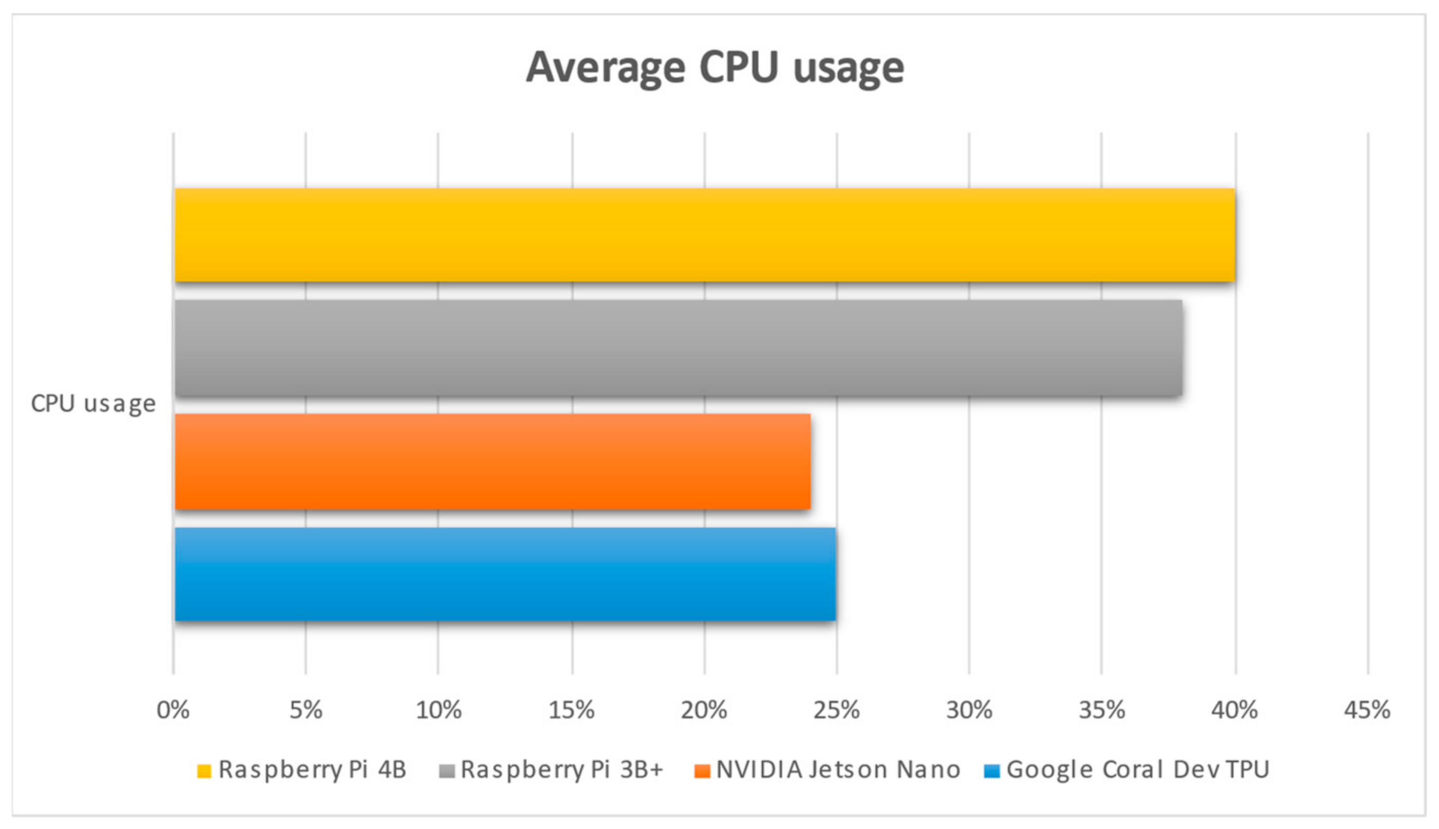
As can be observed in Figure 1, NVIDIA Jetson Nano uses about half the CPU power (25%) that the 2 Raspberry Pi 3 (38%) and Raspberry Pi 4 (40%) use. This is an indication that NVIDIA Jetson Nano is based on its GPU to address the various commands given via the python script, with the related ML model. On the other hand, the two Raspberry devices are CPU-based, enabling them to execute the python code, which accounts for using more CPU resources in respect to the Jetson Nano. Another obvious aspect is the fact that the Google Coral TPU shows the same rationale as NVIDIA Jetson Nano, meaning that it uses fewer CPU resources. However, the fact that NVIDIA Jetson Nano and Google Coral Dev TPU use their CPUs less happens for a different reason. Google Coral TPU uses its ASIC module to execute the various python ML script’s commands related to tensors. The idea is that Google Coral can accelerate the parts of the code which are related to tensors, which are many, since the python code makes use of TensorFlow (Lite) package; thus, it does not need to use more of its CPU power. That is why it uses 25% of its CPU power instead of the 38% and 40% used by the Raspberry Pi 3 and 4.

In Figure 1, it can be observed that Raspberry Pi 4B completed the job in about 244 s and Google Coral did so in 253 s; these times are very close to each other. Jetson Nano completed the job in 275 s and Raspberry Pi 3B+ completed the job in 473 s. It is noticeable that, although the authors’ model has a mean accuracy value in the prediction mode of about 90%, there are two classes (Tomato Septoria Leaf Spot and Tomato Late Blight) that achieved a score of 50%.

As highlighted in the Related Work Section, the authors of [9] achieved a score of 93.33%. The authors of [10] achieved the following scores: for the disease “Bacterial Blight”, they achieved 85.89%; for “Alternaria”, they achieved 84.61%; for “Cerespora”, they achieved 82.97%; for “Grey Mildew”, they achieved 83.78%; for “Fusarium Wilt”, they achieved 82.35%; for “Healthy leaf”, they achieved 80%. In [11], the authors claim that they reached the following scores: (i) for ReLU, 7 × 7, they achieved a testing accuracy of 95.7% in 51 min; (ii) for L-ReU, 7 × 7, they achieved a testing accuracy of 97.3% in 53 min; (iii) for L-ReLU, 11 × 11, they achieved a testing accuracy of 98.0% in 54 min. Lastly, in [12], the authors state that they hit 97% accuracy. Concluding based on the above scores, the average score is around 89.17%, which accounts for the current research results and the claim that “about 90%” is an accepted threshold.

In Figure 2, it can be observed that the 2 Raspberry Pi use more their CPU for the computations, whereas the NVIDIA Jetson Nano and the Google Coral Dev TPU used less CPU because the accelerators were used to a greater extent; CUDA cores were used for the Jetson and ASIC chip was used for the Google Coral.

Figure 2. Average CPU usage for each single-board computer.

Studying the images of these two categories more carefully, it is noted that errors took place because the images are identical and the extraction of different characteristics was quite difficult; for example, the class Tomato Early Blight had identical images and thus the accuracy was 79%, which is less than the mean accuracy of 90%. Unfortunately, although data augmentation was used and despite the authors’ efforts, such issues cannot be easily diminished when there is a small number of images available during the training procedure and given that the classification was performed among 33 labels without connecting identical categories. In Figure 3, the differences among the accuracies accomplished per class can be observed.

Figure 3. Accuracy per class.

Concerning the issue of identical images and the challenges they introduce, since the output of individual characteristics is difficult, an efficient solution can be the collection and usage of higher populations of images per class, which can allow for the efficient filtering of (near-) identical images. The research presented in this paper uses 33 classes, which is a significantly high number concerning the scale of the experiments carried out and the respective hardware used. Nevertheless, as the population of images per class was not that high, the problem of almost-identical images has occasionally been detected. For example, the Tomato Early Blight class included very similar images that led to an accuracy level of 79%, which is significantly lower than the accepted threshold of 90% in the current work.

The diagram in Figure 4 depicts the processing time for each class with the use of Google Colab. The fully equivalent time is achieved with the use of various SBC devices; however, on Raspberry Pi 4, Jetson Nano, and Google Coral Dev Board, the equivalent time is five times higher, and on Raspberry Pi 3B+ it is ten times higher than the time achieved by Google Colab. What is worth mentioning is the total time for implementing the procedure; this is because, in real usage of the algorithm/application, a dataset of non-classified images is chosen. The small time differences per class are a result of the number of images, because the exact same number was not available for all classes, but there was a variance of only ±5 images per classes. The result is presented in order to compare Google Colab with the SBCs, where Google Colab is not an SBC, but is a powerful virtual machine provided by Google for research.

Figure 4. Inference time per class by using Google Colab.

Figure 5 and Figure 6 depict the RAM usage both in MB and in percentage.

Figure 5. Memory usage in percentage when using Pillow.

Figure 6. Memory usage in MBytes when using Pillow.

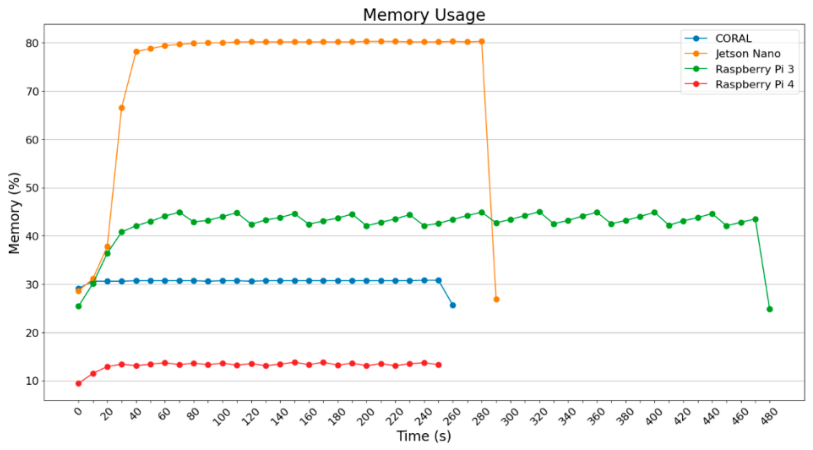
What is remarkable is the fact that Jetson Nano uses a lot of RAM memory, whereas the other devices operate using less than 500 MB. Raspberry Pi 3B+ does not exceed 50% of RAM, Google Coral does not exceed 30%, and Raspberry Pi 4B does not exceed 15%. The results in Figure 5 and Figure 6 are absolutely expected, meaning that Jetson Nano uses GPU most of the time to perform various operations which are energy-consuming.

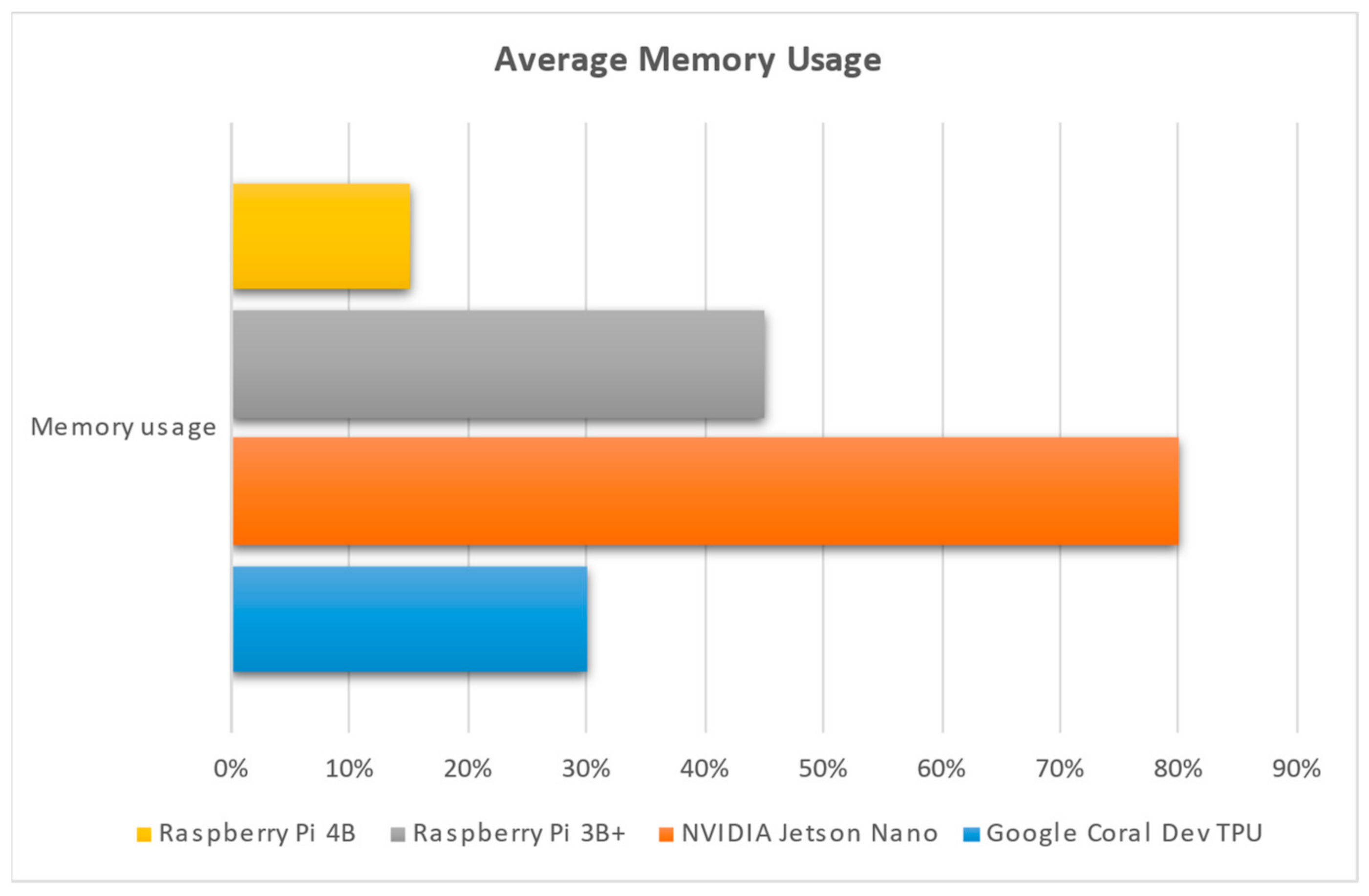
In Figure 7, it can be observed that NVIDIA Jetson Nano uses more of its available RAM (4 GB); this is followed by Raspberry Pi 3B+, which contains 1 GB RAM; next comes Google Coral Dev TPU (1 GB RAM) and then Raspberry Pi 4B (4 GB RAM). In real numbers, NVIDIA Jetson Nano uses 3.2 GB RAM, Raspberry Pi 3B+ uses 450 MB RAM, Google Coral uses 300 MB RAM, and Raspberry Pi 4B uses 600 MB RAM.

Figure 7. Average memory usage for each single-board computer, presented in percentage of its overall memory available.

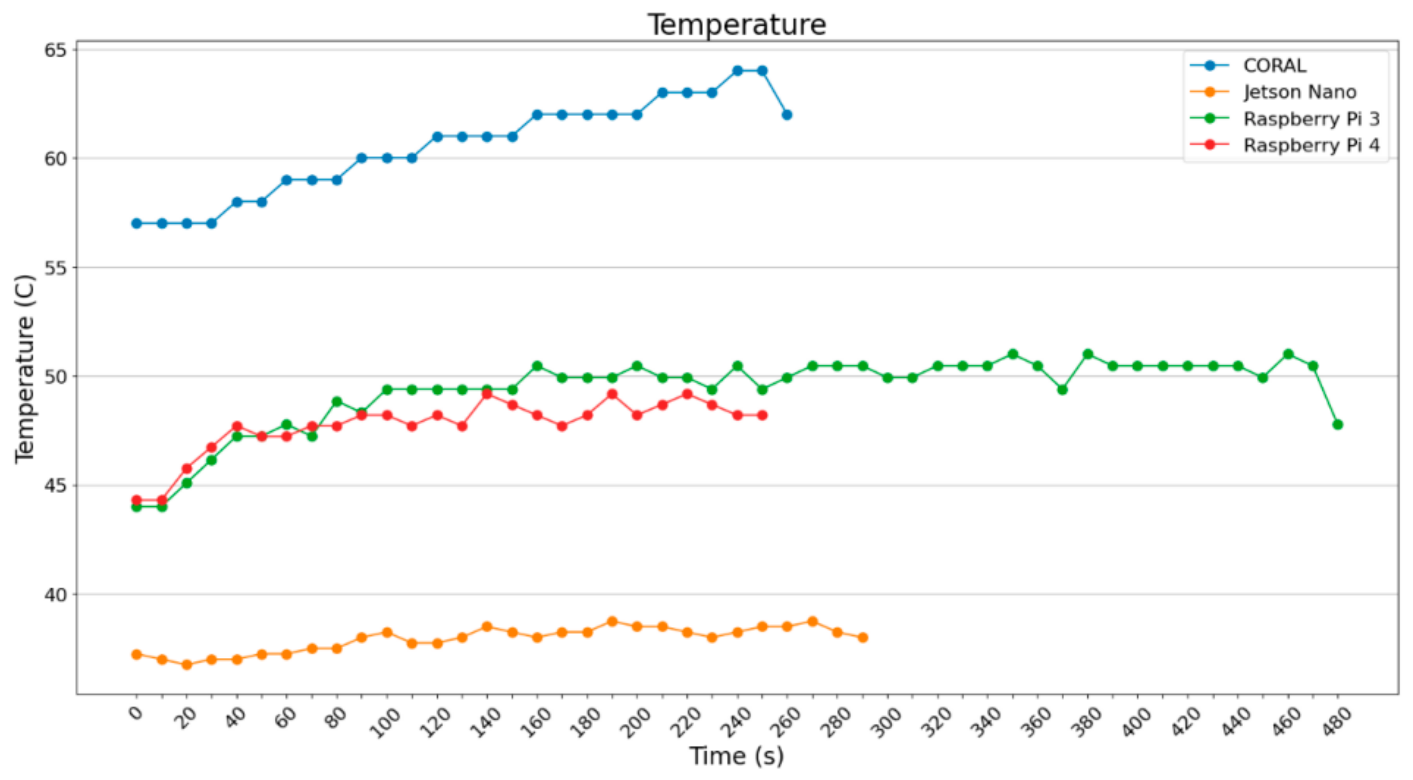
As far as temperature is concerned (Figure 8), Jetson Nano shows very low temperatures when operating, due to its bigger fan and the large heat sink. Google Coral, on the other hand, shows high (but controlled) temperature; apart from the heat sink, the fan did not operate for a considerable amount of time. The fan was activated automatically a few times, when the heat could not be dissipated through the heat sink.

Figure 8. Temperature of the device when using Pillow.

In Figure 9, it can be observed that NVIDIA has the lowest temperature while operating four SBCs. This seems to be the result of a large heatsink and a big fan. Google Coral Dev’s TPU cannot handle the increased temperature of 60 °C, and hits the highest temperature of all four SBCs. The two Raspberry Pi devices hit temperatures between 48 °C and 50 °C, and although they both have heatsinks and fans working continuously, they do not seem to be so effective in dissipating the heat.

Figure 9. Mean temperature of each SBC, presented in Celsius degrees.

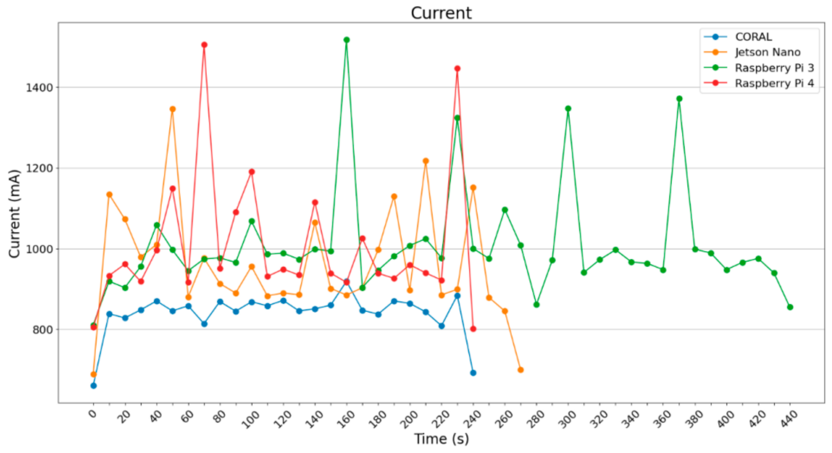
Concerning the current draw, the results are depicted in Figure 10. All four SBCs were supplied with stable 5.1 Volt DC; however, the pictures depict only the current draw. The power can be easily estimated using the following equation:

$$\mathrm{P}\left(\mathrm{p}\mathrm{o}\mathrm{w}\mathrm{e}\mathrm{r}\right(\mathrm{m}\mathrm{W}\left)\right)=5.1\left(\mathrm{V}\mathrm{o}\mathrm{l}\mathrm{t}\right)\cdot \mathrm{I}\left(\mathrm{C}\mathrm{u}\mathrm{r}\mathrm{r}\mathrm{e}\mathrm{n}\mathrm{t}\right(\mathrm{m}\mathrm{A}\left)\right)$$

(1)

Figure 10. Current measurement per device when using Pillow.

All the devices except the Google Coral draw about 1000 mA of current with a few peak values over 1350 mA; the rest of the values are about 800 mA. Due to its architecture, Google Coral achieves very stable values of current draw and power consumption, which are clearly below the respective measurements of the other three devices.

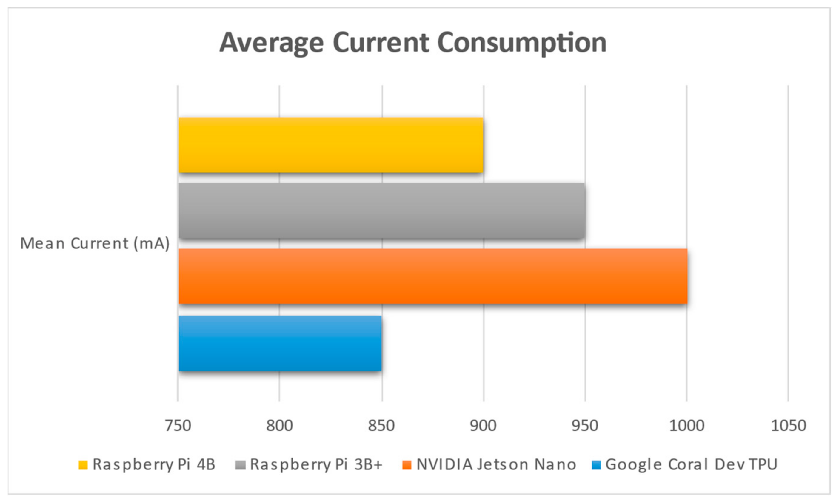
In Figure 11, one can see that NVIDIA Jetson Nano is the most “energy-hungry” device of all four assessed; this is expected, since it is widely known that GPUs consume a lot of power, accounting for the tendency of the scientific community to also use devices such as ASIC or FPGA (field programmable gate arrays) (https://inaccel.com/studio/ (accessed on 20 January 2024)), where the speedup is extreme with low power consumption.

Figure 11. Average current consumption for each single-board computer in mA.

The use of generators apart from the training procedure affects the prediction part as well, where the images were loaded into the model per batch, with the help of generators. Moreover, images are processed in groups of 2, 4, 8, 16, and 32 in this case. For the realization of that experiment, Raspberry 3 and Raspberry 4 were chosen for use, but not Google Coral TPU, because it does not support the common TensorFlow and thus there was no chance of using ImageDataGenerator, which is part of Keras. Keras is an open-source library that provides a python interface for neural networks and it is an interface for TensorFlow library. In addition, neither of the NVIDIA Jetson Nanos were used because their OS did not support such a procedure.

The experiments that took place used batch_size = 2, 4, 8, and 16; only Raspberry Pi 4B+ was tested with batch_size = 32, improving the execution time. What is obvious in the following diagrams is that as the batch_size increases, the execution time decreases; meanwhile, there is a demand for more computational resources. In Figure 12, a diagram for batch_size = 2 is depicted.

Figure 12. CPU usage (ImageDataGenerator—batch size = 2).

For the execution with batch_size = 2, nothing remarkable was noticed, only that Raspberry Pi 4 can implement its process faster. Below, the diagram for batch_size = 4 is depicted.

In Figure 13, what is worth mentioning is that Raspberry Pi 3B+ improved the execution time a bit in comparison to the data in Figure 12; also note that Raspberry Pi 4B improved the time for 80 s, which is significant in relation to the total time. Below, the diagrams for batch_size = 8 and batch_size = 16 are depicted.

Figure 13. CPU usage (ImageDataGenerator—batch size = 4).

In Figure 14 (batch_size = 8), a small improvement is noted, but it remains similar to the previous (Figure 13). In the diagram of Figure 15, however, a significant improvement in execution time for the two Raspberry devices is noted due to the fact that a suitable increase in the images (batch_size) causes a decrease in recursions. That occurs because the algorithm needs to execute fewer iterations.

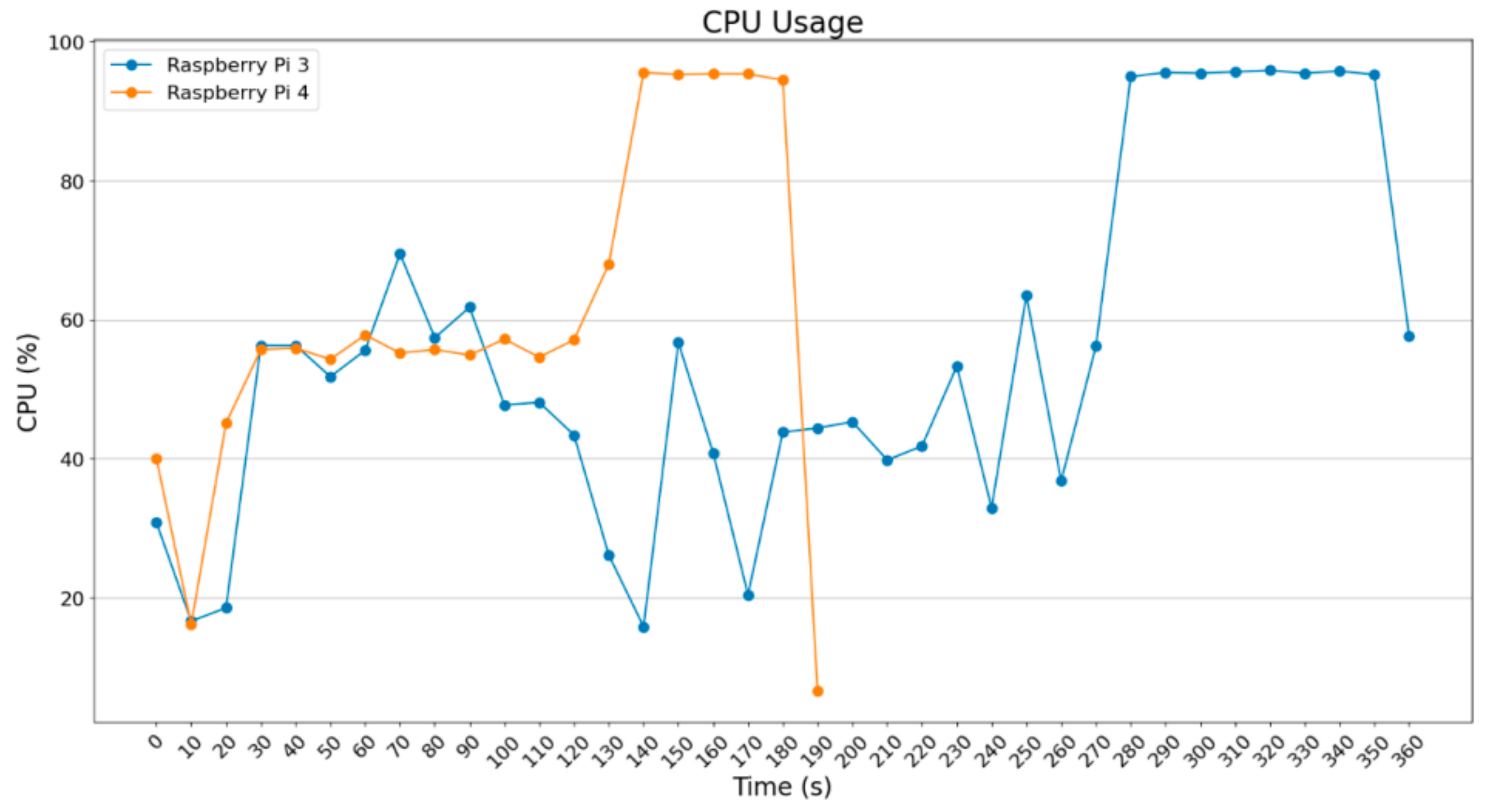
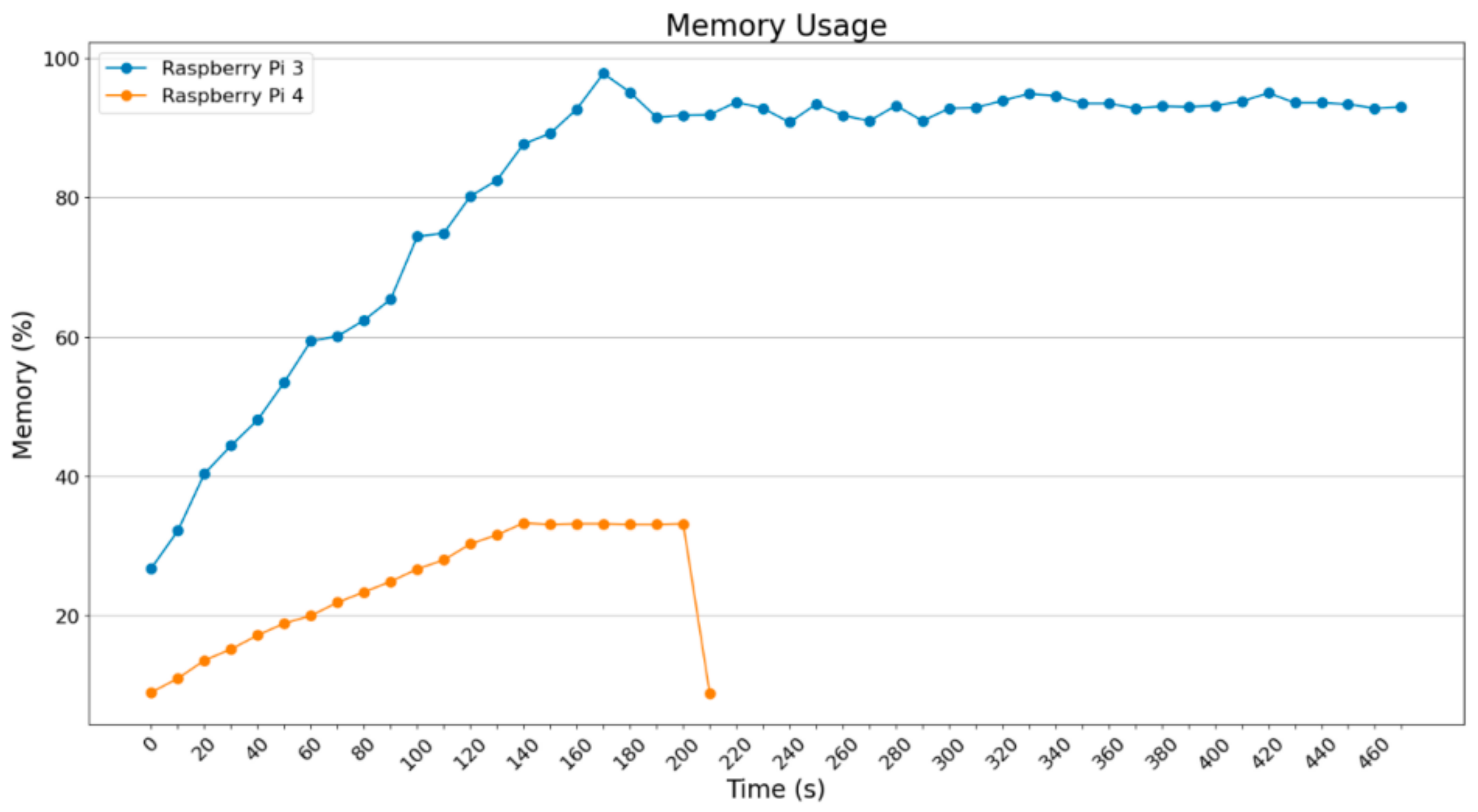
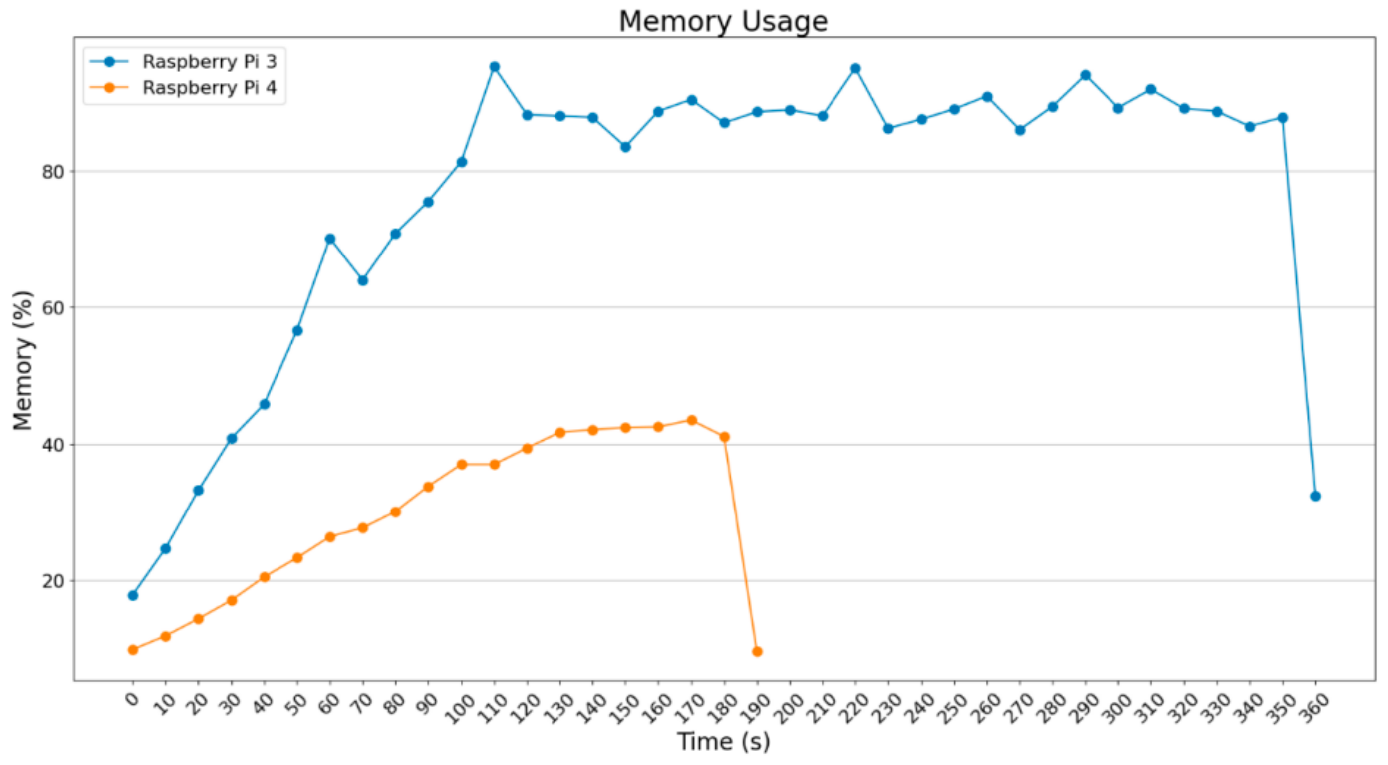
Figure 14. CPU usage (ImageDataGenerator—batch size = 8).

Figure 15. CPU usage (ImageDataGenerator—batch size = 16).

The diagrams below depict the usage of memory for the Raspberry Pi 3B+ and Raspberry Pi 4B. The first diagrams illustrate the memory percentage (Figure 16, Figure 17, Figure 18 and Figure 19) that was used and the diagrams that follow present the memory usage in MBytes (Figure 20, Figure 21, Figure 22 and Figure 23).

Figure 16. Memory usage (percentage) (ImageDataGenerator—batch size = 2).

Figure 17. Memory usage (percentage) (ImageDataGenerator—batch size = 4).

Figure 18. Memory usage (percentage) (ImageDataGenerator—batch size = 8).

Figure 19. Memory usage (percentage) (ImageDataGenerator—batch size = 16).

Figure 20. Memory usage (MBytes) (ImageDataGenerator—batch size = 2).

Figure 21. Memory usage (MBytes) (ImageDataGenerator—batch size = 4).

Figure 22. Memory usage (MBytes) (ImageDataGenerator—batch size = 8).

Figure 23. Memory usage (MBytes) (ImageDataGenerator—batch size = 16).

In Figure 16, Figure 17, Figure 18 and Figure 19, it is obvious that RAM usage for the Raspberry Pi 3B+ remains high at about 90%. Theoretically, it was expected that the Raspberry Pi 3B+ could not finalize those procedures given the extra load. However, as will be shown below, apart from the marginal usage of RAM, extra memory was enabled. Raspberry Pi 4B does not face any difficulty as the Raspberry Pi 3B+ does. It reached 30–40% RAM usage, so that it could process and accelerate the operations.

Below, diagrams related to RAM usage are examined, based on capacity this time.

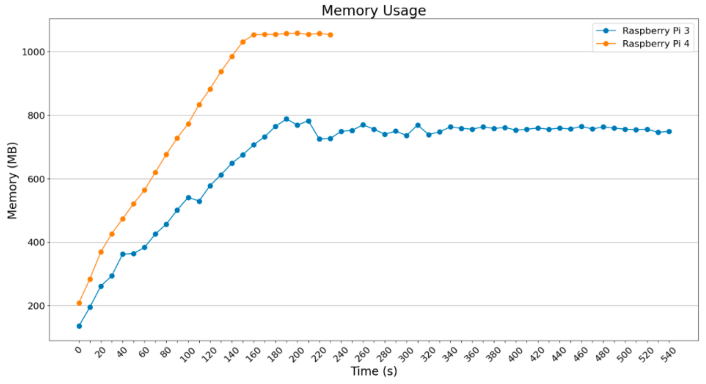
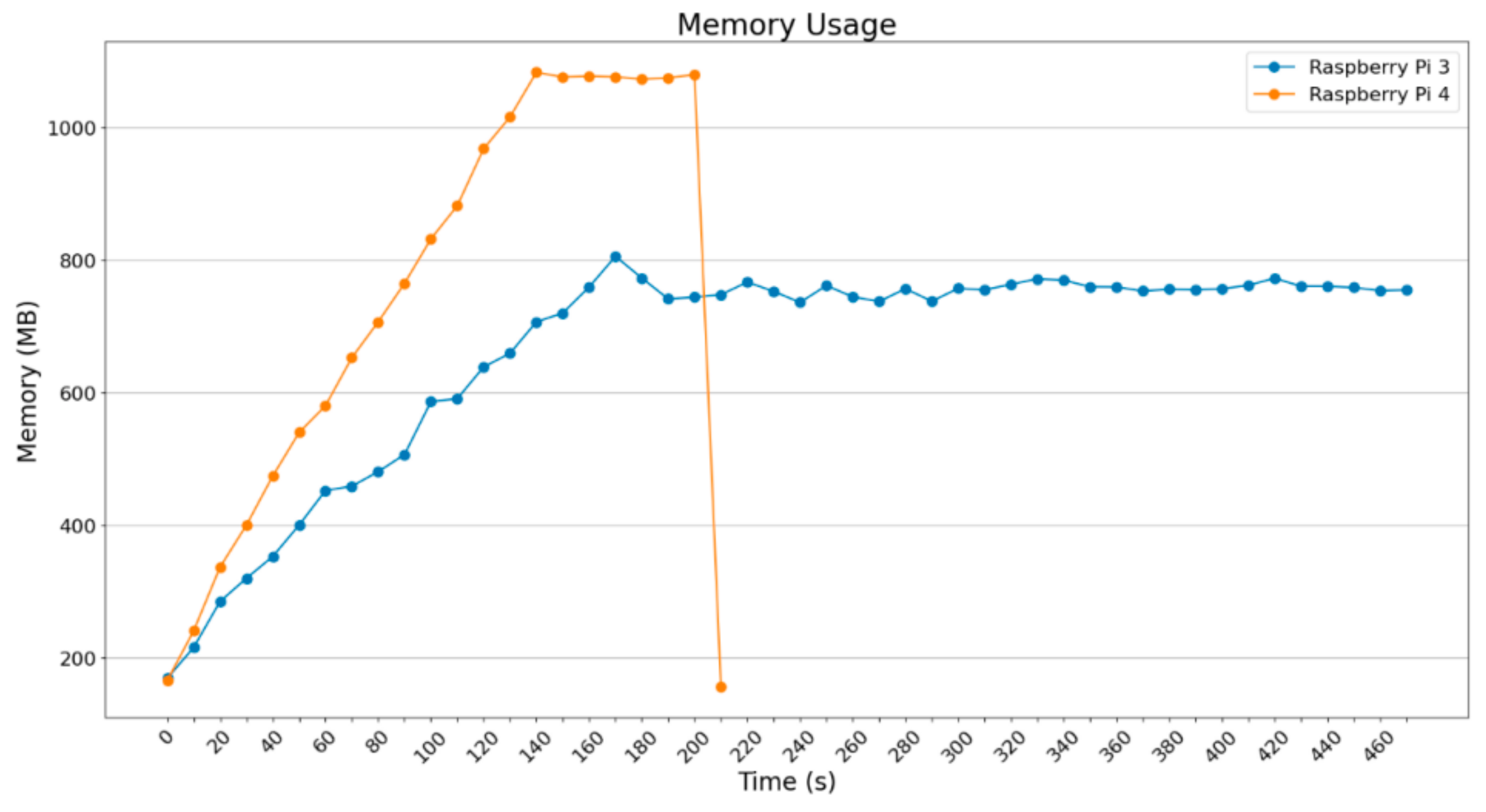
In Figure 20 and Figure 21, the RAM usage for batch_size = 2 and batch_size = 4 are depicted in MBytes. Raspberry Pi 3B+ uses around 800 MBytes, which is almost all of the available RAM (875 MB is the maximum available). Raspberry Pi 4B uses more MBytes because the maximum available is about 4 GB, something that makes it the most powerful IoT device, which is obvious from the execution time of the processes.

Figure 22 and Figure 23 depict the usage of memory in MBytes in two of the heaviest situations that have been presented until this point; these are related to batch_size = 8 and batch_size = 16.

What is obvious in Figure 22 and Figure 23 is that the Raspberry Pi 4B starts being stressed in comparison to the previous situations since the memory demands increase, given that it loads and processes 8 and 16 images, reaching 1250 MBytes and 1500 MBytes RAM. Raspberry Pi 3B+ seems to be stressed under the load it was assigned to.

As far as temperature is concerned, nothing special was noticed; the variance was stable.

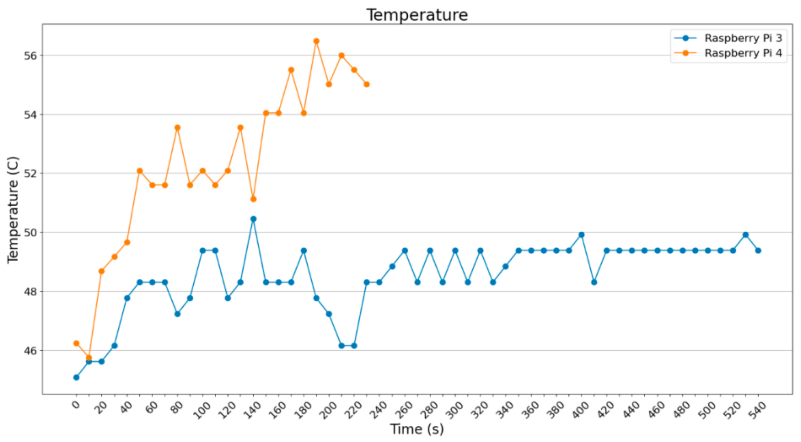
For batch_size = 2 (Figure 24) and batch_size = 4 (Figure 25), it is noted that Raspberry Pi 3B+ was operating steadily at about 49 °C, whereas the Raspberry Pi 4B showed an intense increase from 45 °C to 55 °C.

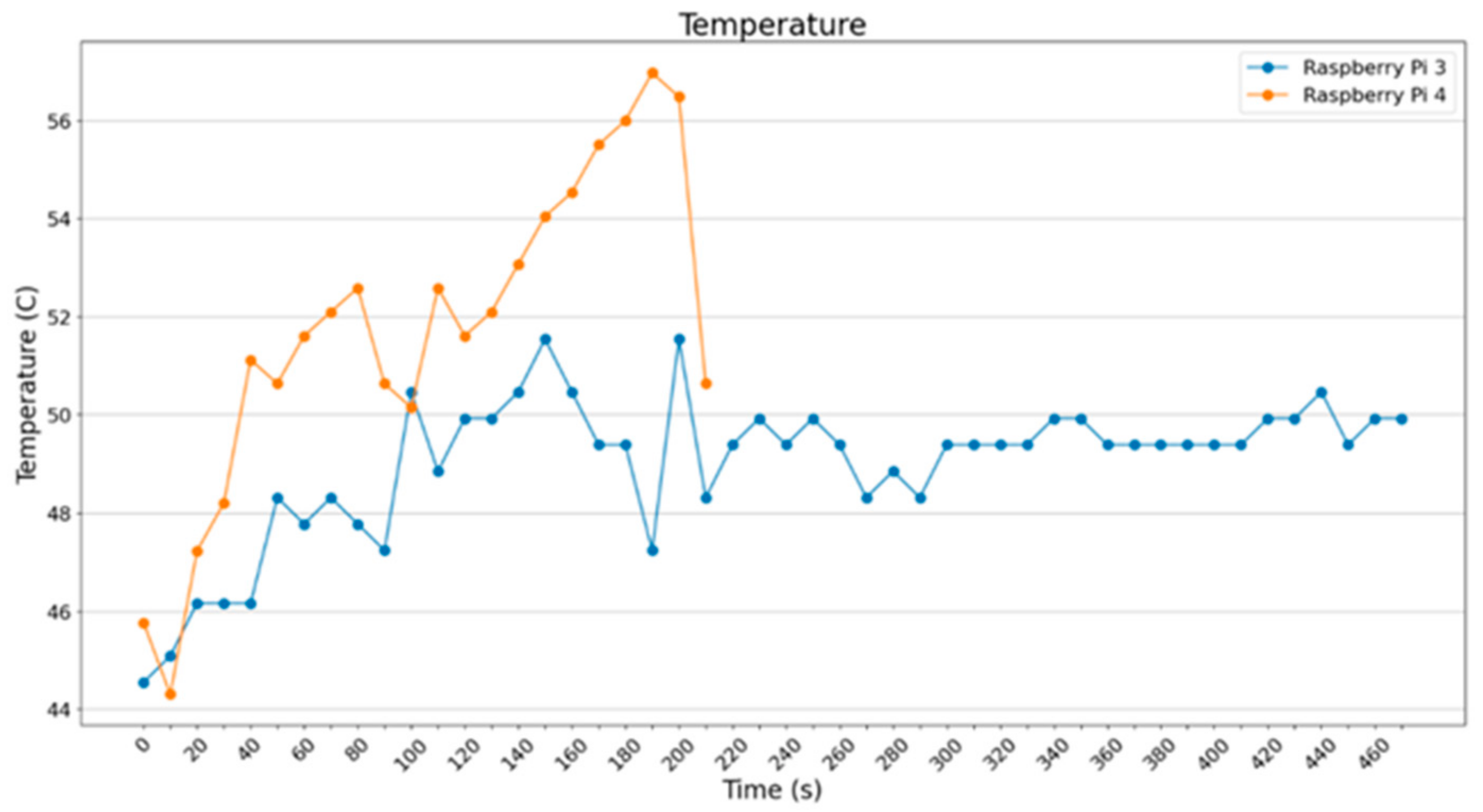
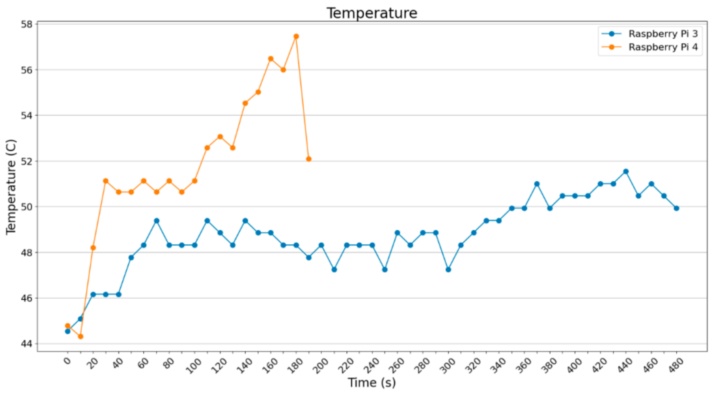
Figure 24. Temperature of devices (ImageDataGenerator—batch size = 2).

Figure 25. Temperature of devices (ImageDataGenerator—batch size = 4).

In Figure 26 and Figure 27, the cases for batch_size = 8 and batch_size = 16 are shown. It is noted that Raspberry Pi 3B+ remains at 49 °C with spike at the end, which is expected since it is quite loaded to operate smoothly, concerning both RAM and CPU usage. Regarding Raspberry Pi 4B, it is noted that it starts operating smoothly but it ends up stressed.

Figure 26. Temperature of devices (ImageDataGenerator—batch size = 8).

Figure 27. Temperature of devices (ImageDataGenerator—batch size = 16).

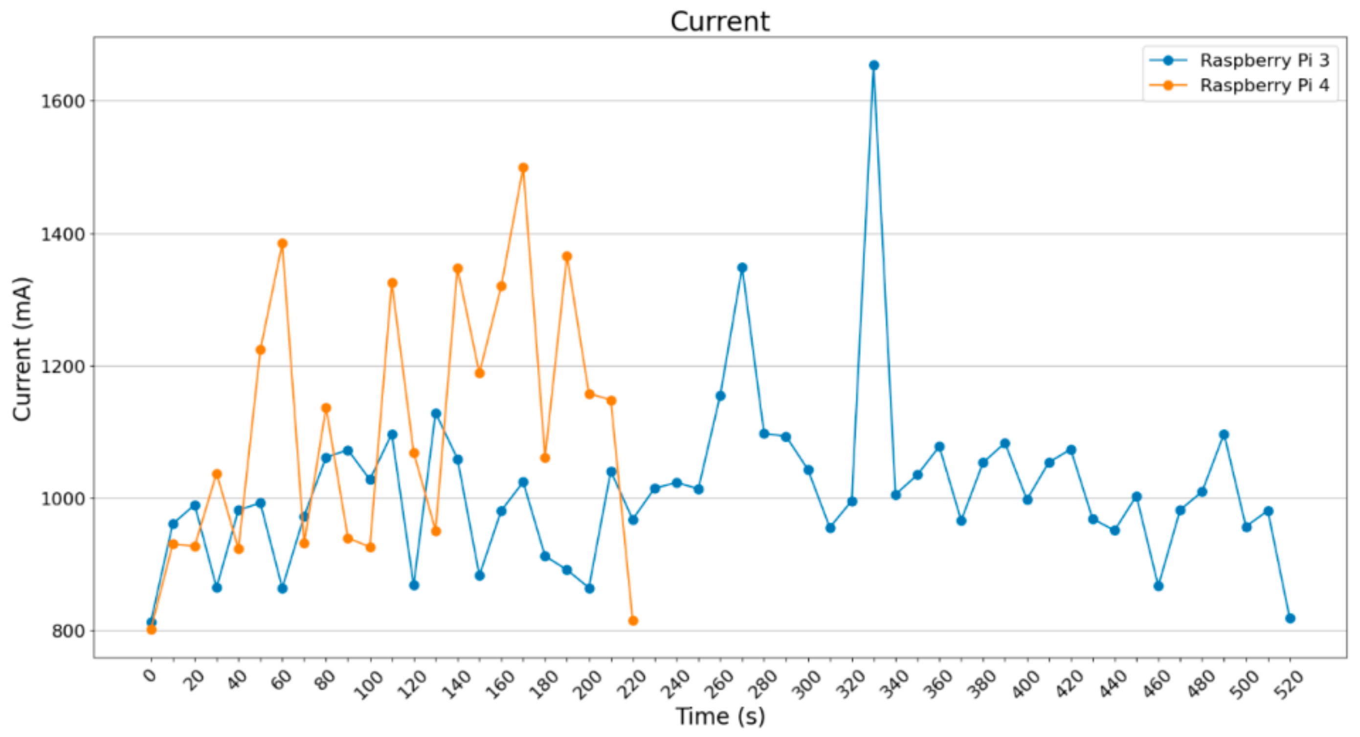
As far as the current draw per batch_size is concerned (i.e., the temperature graphs mentioned before), the same thing occurs in current draw as well, meaning that the more the batch_size increases, the more the SBCs are stressed. Consequently, power consumption is higher. Current draw mean value starts from around 1050 mA for batch_size = 2 to 1200 mA for batch_size = 16 in Raspberry Pi 4B. In Raspberry Pi 3B+, higher extreme values are observed.

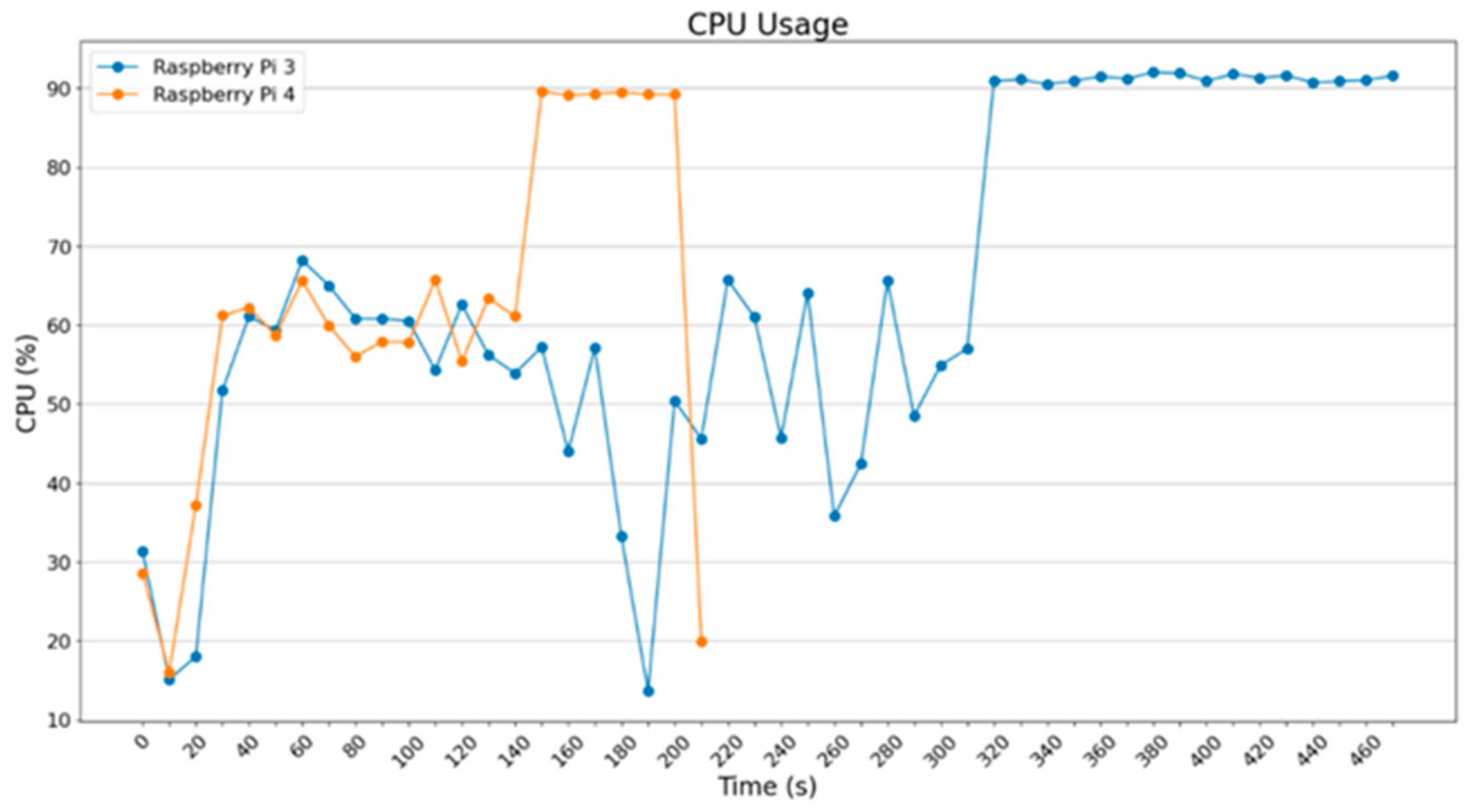
In the below diagram (Figure 28), many spikes are noted for Raspberry Pi 4B but not that many are noted for Raspberry Pi 3B+.

Figure 28. Current metric (mA) (ImageDataGenerator—batch size = 2).

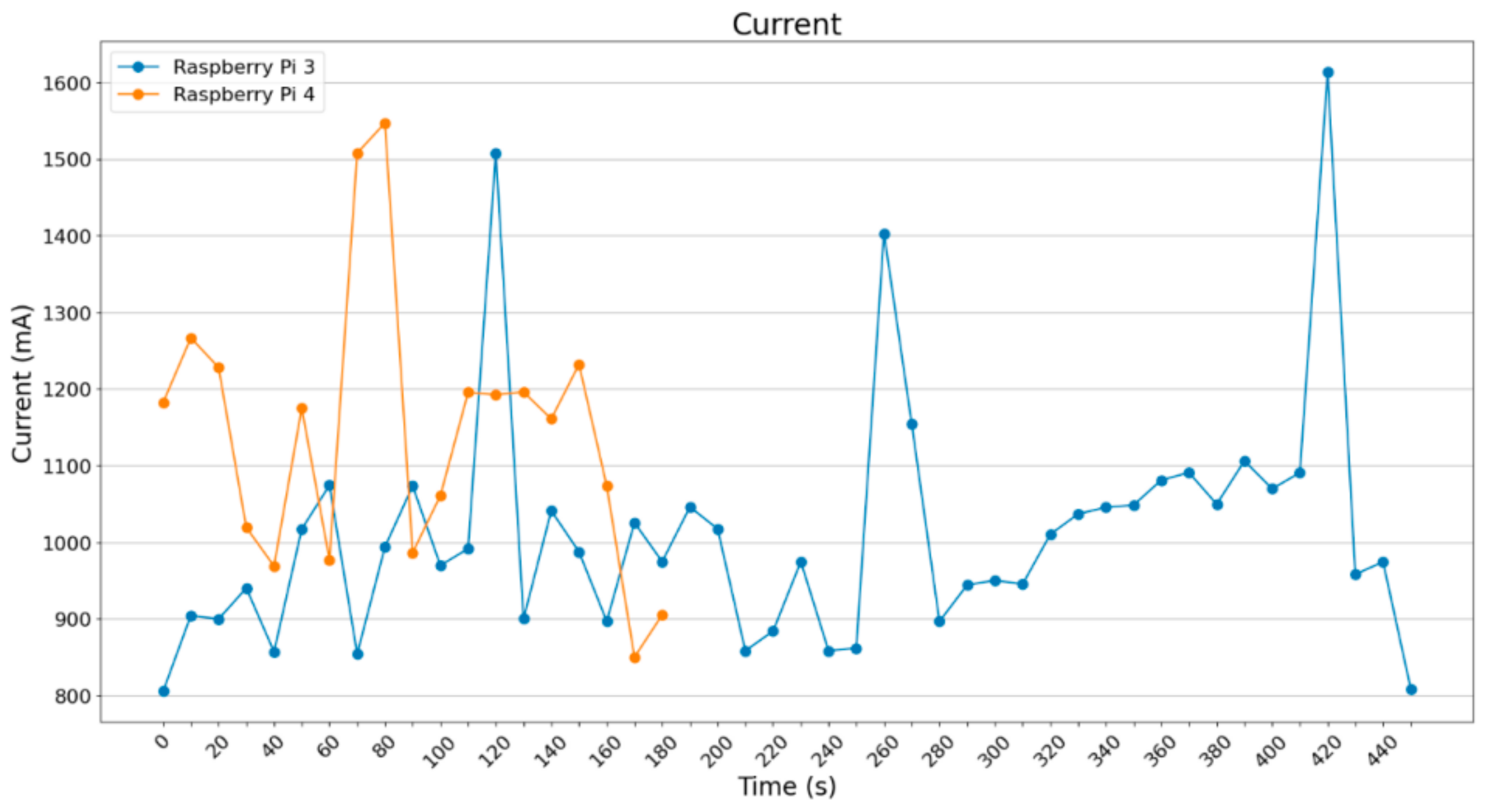
For batch_size = 4 (Figure 29), a small increase in current draw can be noticed in the Raspberry Pi 4B around 1200 mA. Raspberry Pi 3B+ starts getting stressed, with spikes over 1500 mA. Below, the graph for batch_size = 8 (Figure 30), showing a small current increase on both Raspberry Pi 3B+ and Raspberry Pi 4B.

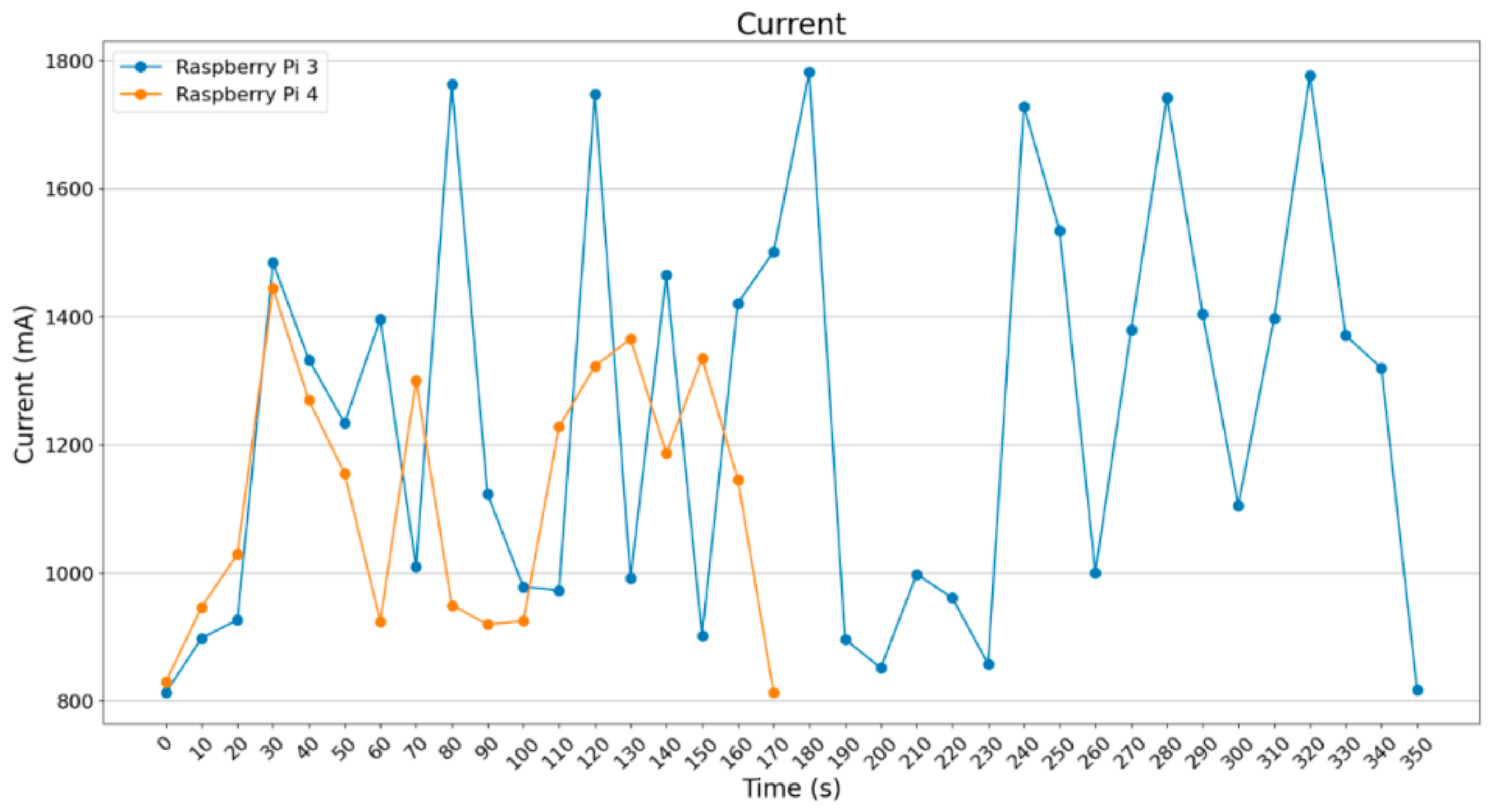
Figure 29. Current metric (mA) (ImageDataGenerator—batch size = 4).

Figure 30. Current metric (mA) (ImageDataGenerator—batch size = 8).

In Figure 31, a significant difference is depicted between the more powerful Raspberry Pi 4B and the Raspberry Pi 3B+. In the case of batch_size = 16, a small increase in current is noted in relation to batch_size = 8. However, Raspberry Pi 3B+ exceeded 1700 mA in more than half of the values sampled, whereas Raspberry Pi 4B was operating at around 1200 mA.

Figure 31. Current metric (mA) (ImageDataGenerator—batch size = 16).

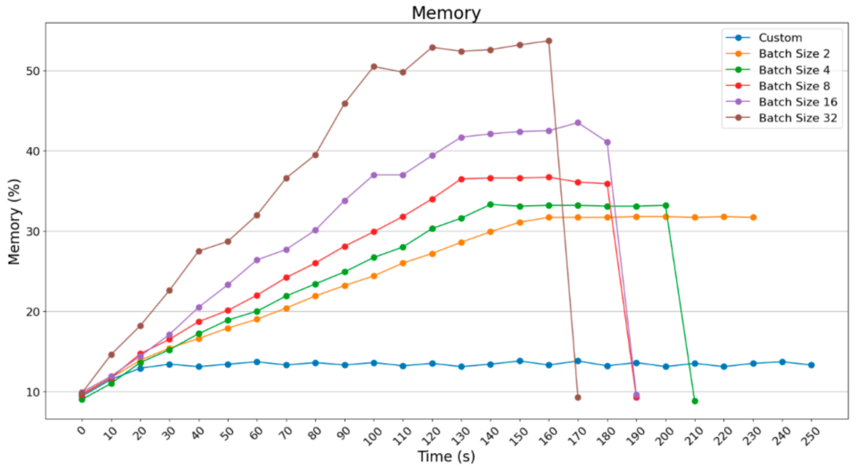
Next, Figure 32 depicts how the Raspberry Pi 3B+ and Raspberry Pi 4B use the batch_size in different sizes and how each device is compared to itself given the executions including the Pillow technique. Starting with Raspberry Pi 3B+, the diagrams below were drawn; it is clear that, for the purpose of improving execution time, more resources were necessary, particularly for batch_size = 16.

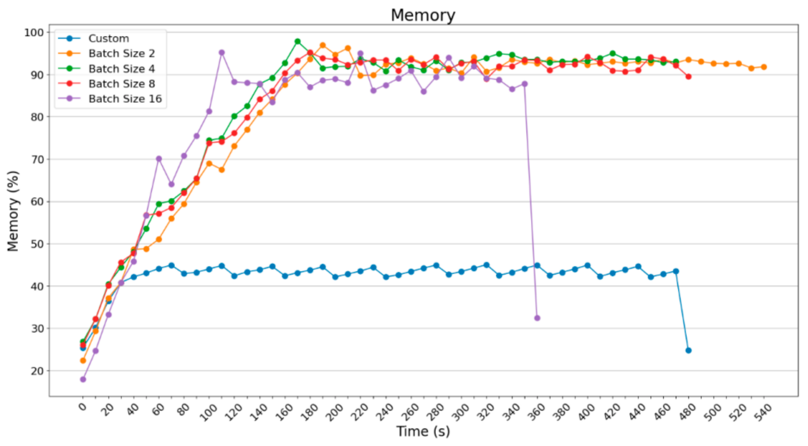
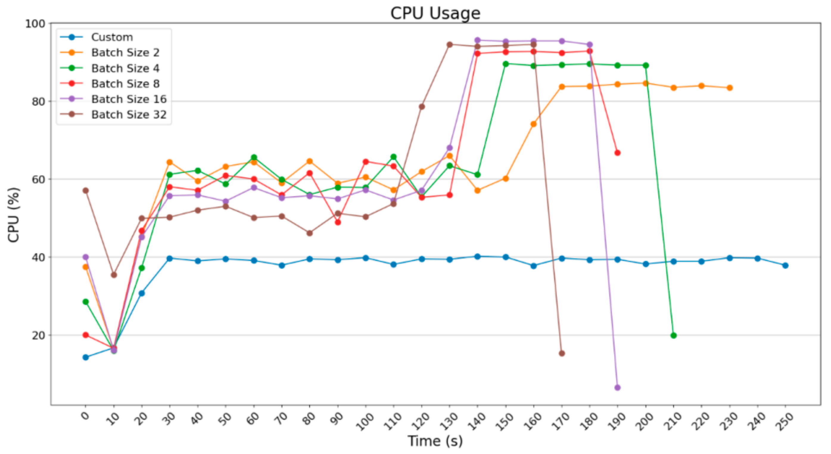
Figure 32. Raspberry Pi 3B+ CPU usage.

Diagrams in Figure 32 and Figure 33 depict the following: the usage of RAM memory and CPU for Raspberry Pi 3B+ based on different executions. What is noticeable is that the usage of a custom solution on loading images one-by-one does not rewire the use of many computational resources, reaching the end result. However, with the use of ImageDataGenerator, good use of images per batch was possible; thus, there was a marginal decrease in the execution time of processing per group.

Figure 33. Memory usage when using Raspberry Pi 3B+ in percentage.

The next diagram (Figure 34) shows the memory usage in MBytes; it is equivalent with the diagram of the percentage of memory RAM use.

Figure 34. Memory usage when using Raspberry Pi 3B+ in Mbytes.

The diagram that follows (Figure 35) depicts the additional need as a result of the larger group on loading images, because a bigger memory is required. As is shown, Raspberry Pi 3B+ almost doubles the memory it uses by adding 750 MB Swap to complete the procedures in the more computationally difficult but faster situation.

Figure 35. Swap memory usage using Raspberry Pi 3B+ in MBytes.

The difference in execution time with batch_size = 16 is obvious, the difference in usage of computation resources is observable too. With regard to temperature (Figure 36), there were no intense outputs, since time differs significantly with batch_size = 16. The batch_size = 32 For Raspberry Pi 4B was tried and, as will be shown in the following Figure 37 and Figure 38, output faster results, making good use of computational resources.

Figure 36. Temperature in Raspberry Pi 3B+.

Figure 37. CPU usage in Raspberry Pi 4B.

Figure 38. Memory usage in percentage when using Raspberry Pi 4B.

As far as the usage of computational power is concerned, there is not a significant difference between the experiments with the use of ImageDataGenerator. However, the usage of computational power is significant compared to the custom prediction.

In Figure 39, an acceleration of about 20 s took place when batch_size = 3 was used. However, for acceleration concerning the execution time (by doubling the amount of the images per group), the percentage of memory exceeds 50%. Respectively, in Figure 39, RAM in MBytes excels 1800 MBytes; in contrast, in the previous cases, it did not exceed 1500 MBytes.

Figure 39. Memory usage in MBytes when using Raspberry Pi 4B.

In Figure 40, it can be observed that the temperature readings do not show an essential difference between the cases, as the Raspberry Pi 4B maintains a temperature of around 52 °C in all scenarios.

Figure 40. Temperature when using Raspberry Pi 4B.

Apart from the obvious improvement in execution time with batch_size = 32 and the necessary increase mainly in the memory resources, it is worth noticing that Raspberry Pi 4B can easily implement the process of prediction with Pillow, which stands for the custom way of loading images one-by-one with the use of ImageDataGenerator, although it requires 80 s more.

As can be observed from the graph, Raspberry Pi 4B is the fastest of all the four SBCs regarding the time completion of the task; as has been discussed in a previous section, it takes about 244 s to finish the task, i.e., the inference part of the ML model. The slowest hardware is that of the Raspberry Pi 3B+, taking about 453 s to complete the job. Raspberry Pi 4B uses 4 GB RAM and a more powerful processor: Broadcom BCM2711, quad-core Cortex-A72 (ARM v8) 64-bit SoC @ 1.5 GHz. This is in comparison to Raspberry’s Pi 3B+ CPU: Broadcom BCM2837B0, Cortex-A53 64-bit SoC @ 1.4 GHz. This is depicted in Figure 41. The Raspberry Pi 3B+ also uses 1 GB RAM, which is significantly lower than the 4 GB RAM that Raspberry Pi 4B uses. Although it would be expected that NVIDIA Jetson Nano is the fastest of all four modules, it is evident that it is not. TPU and GPU, however, use less CPU power than the Raspberry Pi devices, which are CPU-centered.

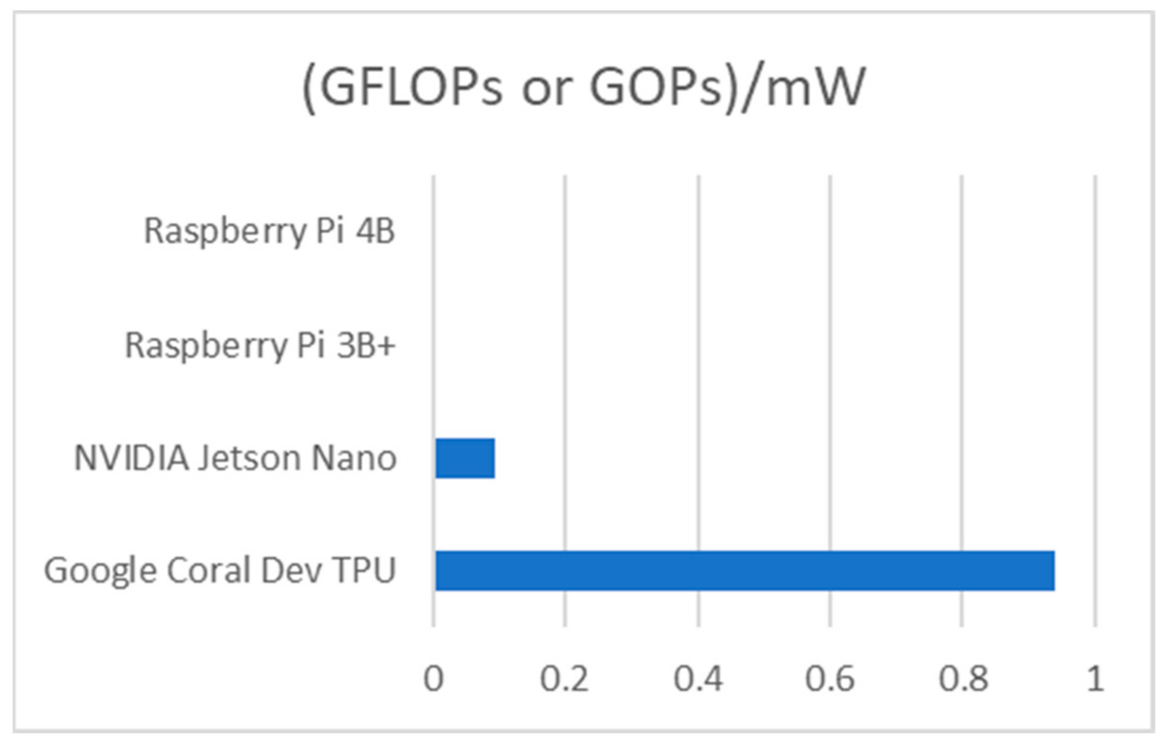
Figure 41. Completion time of the inference part handled by each SBC.

As is seen from Table 2, concerning the inference part, the Google Coral Dev TPU is the most efficient, followed by NVIDIA Jetson Nano. Next comes the Raspberry Pi 3B+, and the last and least efficient module is the Raspberry Pi 4B. In Figure 42, it is clear that Google Coral Dev TPU is by far the most efficient of all four SBCs.

Table 2. Efficiency analysis of each SBC module, given the GFLOPs or GOPs vs. power consumption (in mWatts).

SBC	Mean Current (mA)	Voltage (Volts)	Power (mW)	GFLOPs or GOPs 1	(GFLOPs or GOPs)/mW
Google Coral Dev TPU	850	5	4250	4000	0.9411
NVIDIA Jetson Nano	1000	5	5000	472	0.0944
Raspberry Pi 3B+	950	5	4750	5.3	0.0011
Raspberry Pi 4B	900	5	4500	9.69	0.0021

¹ GFLOPs stands for Giga (10⁹) floating point operations per second and is applied to Raspberry Pi 3B+, Raspberry Pi 4B, and NVIDIA Jetson Nano. GOPs stands for Giga (10⁹) operations per second and is applied to Google Coral Dev TPU.

Figure 42. Giga (10⁹) floating points operations per second or Giga operations per second per 1 mWatt power consumption for each SBC.

5.2. Limitations and Challenges in the Current Work

When working with code running in SBCs, it is critical to write a python code that takes the various CPU/GPU/TPU constraints, the mitigated RAM memory, and the diminished ROM capabilities into consideration. A serious aspect is the fact that the initial python ML code was trained in Google Colab, which has powerful GPU modules and offers extreme parallelization in the implemented code. It is very difficult—and most times prohibitive—to train an ML model in SBCs, because it takes too many hours. SBCs have many constraints making training of ML models infeasible. There are CPU mitigations, RAM memory mitigations, swap memory mitigations, HDD constraints, and power constraints. Experience in the past has shown that, although training in GPU-based SBCs consumes less time than CPU-based SBCs, it is not recommended at all. Another issue addressed was the fact that Google Coral TPU does not support the TensorFlow python package, which is one of the mainstream solutions on writing ML python code. However, it supports the TensorFlow Lite package. For this reason, the code to be executed in Google Coral TPU had to be changed and be explicitly configured for this purpose, without losing its rationale.

5.3. Overall Experimental Evaluation Findings

Below, an analysis of the various constraints that were faced when working with dataset of the images, as well as possible solutions, is presented. There is also a discussion of the effect of temperature on the construction and the respective means to mitigate the effects. Lastly, we present the findings of our experience of how GPU and TPU accelerators behave in large-scale systems during the training phase, which unfortunately is not crystal clear in constrained-resource SBCs.

In the image processing part, the implementations that we studied until the time of writing the current subsection (2024) have been realized; they refer to one kind of leaf, that was divided into the basic leaf classes. In the current research, various leaves were used and were divided into more classes, rather than using one leaf, since there are different kinds of plants in an image depicting only one crop; thus, a generalized approach is needed. There was an effort to use real images and not perfected ones, which explains why there were light variations and other human-made conditions, making the model more efficient in real case prediction. The result from the metrics was as follows: GPUs are an “energy-hungry” solution. They may be good accelerators since they can implement extreme parallelization in their CUDA cores and decrease the completion time of a process, but they consume more energy in comparison to the other SBCs used in the current experiments. Raspberry Pi 4B is considered to be faster than the older Raspberry Pi 3B+ when completing a task; however, both are CPU-based, meaning that a lot of time is required in large ML models since they do not use accelerators. Google Coral Dev TPU is really “fast” in completing a task; this is because it mainly uses less CPU power and less energy in comparison with a GPU-based SBC, as it accelerates specific parts of the python code. However, changes in both the code and the models are necessary in order to progress, because the Google Coral Dev TPU does support the TensorFlow package.

Increased temperatures show that the SBC consumes a lot of power (current draw). This is very critical when there is a need to use an SBC far from wall plug electricity. To be more specific, when it is necessary to operate the SBC in a place where the power comes from a battery combined with a small solar panel or a small wind generator, there will be power supply constraints. Attention should be paid to use as little power as possible, because all the power will come from a battery that can be depleted too quickly. Another consequence of increased temperatures in an SBC is that there should be a configuration in the hardware in order to dissipate all the heat, meaning the use of a small fan, or two if the SBC is enclosed in a project box, becomes necessary. Moreover, the use of heatsinks on the CPU/GPU/TPU chip with specific glues dissipating the heat seems vital. The worst-case scenario appears when such SBC devices need to operate during the summer or hot months that add an extra burn due to the heat emitted by the chip. For this reason, bigger fans need to be used, adding an additional current load to the whole circuit device (fans consume more current); therefore, the battery depletes faster.

Experience with large-scale training ML models in Google Colab VM has shown that a GPU can offer acceleration in the training period of an ML model in comparison to a CPU. The idea is that a GPU is highly parallelizable, with thousands of threads working in parallel, whereas a CPU operates sequentially and consumes much more time than a GPU does. During the training phase, there is also the solution of a TPU, which accelerates the ML model in comparison to the CPU, depending on the number of tensors used.

6. Conclusions and Future Plans

This paper introduced an innovative approach in the agriculture sector that aims to assist users in improving the management of resources and support decision-making processes. Initially, an ML-based image processing application was introduced to classify plant photos across 33 classes of leave diseases; an accuracy of about 90% was demonstrated. Compared to the performance of related state-of-the-art approaches, the proposed solution proves to be more effective in principle. The authors attempted classification across numerous clusters, which significantly increased the difficulty of the respective work; previous research that achieved over 90% accuracy used fewer categories. Moreover, this paper also demonstrated that, with the help of generators and data augmentation, the necessary time for training and model development was reduced; this is also valid for the model-based knowledge extraction time when using IoT devices with reduced resources (SBCs).

Moreover, as far as image processing is concerned, this paper elaborated on a series of experiments engaging IoT devices, with the aim of recording power consumption and current draw. The respective metrics have been selected for further study, as there is occasionally the need to construct a larger cluster using such devices. Moreover, energy constraints and, in general, resource consumption and limitations, are of critical importance. It has thus been observed that the acceleration of procedures made the devices increasingly energy-demanding. Therefore, it depends on the studied use-case and it is up to the developer to select the optimal trade-off between demonstrated performance and consumed resources.

Finally, as concluded in the Related Work Section, ML models targeting the agricultural domain or different fields executed on SBCs with low power solutions have demonstrated several limitations. This is mainly due to the fact that CPU, TPU, and GPU are much less powerful than desktop PCs, especially when Cloud computing resources are used. This has significant consequences regarding the completion time of the inference task, as observed in the related graphs in Section 5. Another critical factor is the fact that low-power hardware is escorted by limited RAM; currently, the RAM in SBCs ranges from 1 GB to 4 GB; this introduces another constraint in the field targeted by this paper. In the hardware solutions used, when the proposed approach needs to operate by exclusively using battery power supply instead of a wall plug, it is recommended to supplement the battery energy source with a small solar panel or a small wind generator, especially for the NVIDIA Jetson Nano, which is the most “energy-hungry” of all the four SBCs studied here. It should be mentioned that cooling solutions are recommended when the targeted hardware devices are used, especially during summer periods, which of course demands an additional power consumption overhead corresponding to the operation of cooling fans. As is clearly demonstrated by the graphs in Section 5, when the batch_size increases, the completion time decreases, but more resources are required leading to the devices being stressed.

The future research plans of the authors include the extension of the image classifier so that it exploits UAVs sending images in real time over an agricultural area. These images will be collected by a remote IoT device that uses the extended application, planned to help real-time decision-making processes concerning the diseases of leaves. The decision making will be coupled with various environmental and agricultural measurements obtained by IoT infrastructure elements. Finally, the authors plan to investigate whether the proposed image clustering approach can be suitably adopted to be usable in other smart farming applications and support decisions regarding, for example, optimal irrigation or fertilization.

References

1. Kim, H.; Nam, H.; Jung, W.; Lee, J. Performance Analysis of CNN Frameworks for GPUs. In Proceedings of the 2017 IEEE International Symposium on Performance Analysis of Systems and Software (ISPASS), Santa Rosa, CA, USA, 24–25 April 2017; pp. 55–64. [Google Scholar]
2. Krizhevsky, A.; Sutskever, I.; Hinton, G.E. ImageNet Classification with Deep Convolutional Neural Networks. Commun. ACM 2017, 60, 84–90. [Google Scholar] [CrossRef]
3. Russakovsky, O.; Deng, J.; Su, H.; Krause, J.; Satheesh, S.; Ma, S.; Huang, Z.; Karpathy, A.; Khosla, A.; Bernstein, M.; et al. ImageNet Large Scale Visual Recognition Challenge. Int. J. Comput. Vis. 2015, 115, 211–252. [Google Scholar] [CrossRef]
4. Hara, K.; Saito, D.; Shouno, H. Analysis of Function of Rectified Linear Unit Used in Deep Learning. In Proceedings of the 2015 International Joint Conference on Neural Networks (IJCNN), Killarney, Ireland, 12–17 July 2015; pp. 1–8. [Google Scholar]
5. Bottou, L. Online Learning and Neural Networks; Cambridge University Press: Cambridge, UK, 1998. [Google Scholar]
6. Douarre, C.; Schielein, R.; Frindel, C.; Gerth, S.; Rousseau, D. Deep Learning Based Root-Soil Segmentation from X-ray Tomography. Plant Biol. 2016. [Google Scholar] [CrossRef]
7. Chen, S.W.; Shivakumar, S.S.; Dcunha, S.; Das, J.; Okon, E.; Qu, C.; Taylor, C.J.; Kumar, V. Counting Apples and Oranges With Deep Learning: A Data-Driven Approach. IEEE Robot. Autom. Lett. 2017, 2, 781–788. [Google Scholar] [CrossRef]
8. Rahnemoonfar, M.; Sheppard, C. Deep Count: Fruit Counting Based on Deep Simulated Learning. Sensors 2017, 17, 905. [Google Scholar] [CrossRef] [PubMed]
9. Nalawade, R.; Nagap, A.; Jindam, L.; Ugale, M. Agriculture Field Monitoring and Plant Leaf Disease Detection. In Proceedings of the 2020 3rd International Conference on Communication System, Computing and IT Applications (CSCITA), Mumbai, India, 3–4 April 2020; pp. 226–231. [Google Scholar]
10. Sarangdhar, A.A.; Pawar, V.R. Machine Learning Regression Technique for Cotton Leaf Disease Detection and Controlling Using IoT. In Proceedings of the 2017 International conference of Electronics, Communication and Aerospace Technology (ICECA), Coimbatore, India, 20–22 April 2017; pp. 449–454. [Google Scholar]
11. Jiang, D.; Li, F.; Yang, Y.; Yu, S. A Tomato Leaf Diseases Classification Method Based on Deep Learning. In Proceedings of the 2020 Chinese Control And Decision Conference (CCDC), Hefei, China, 22–24 August 2020; pp. 1446–1450. [Google Scholar]
12. Li, X.; Rai, L. Apple Leaf Disease Identification and Classification Using ResNet Models. In Proceedings of the 2020 IEEE 3rd International Conference on Electronic Information and Communication Technology (ICEICT), Shenzhen, China, 13 November 2020; pp. 738–742. [Google Scholar]
13. Suzen, A.A.; Duman, B.; Sen, B. Benchmark Analysis of Jetson TX2, Jetson Nano and Raspberry PI Using Deep-CNN. In Proceedings of the 2020 International Congress on Human-Computer Interaction, Optimization and Robotic Applications (HORA), Ankara, Turkey, 26–27 June 2020; pp. 1–5. [Google Scholar]
14. Liu, X.; Cao, C.; Duan, S. A Low-Power Hardware Architecture for Real-Time CNN Computing. Sensors 2023, 23, 2045. [Google Scholar] [CrossRef] [PubMed]
15. Zamir, M.; Ali, N.; Naseem, A.; Ahmed Frasteen, A.; Zafar, B.; Assam, M.; Othman, M.; Attia, E.-A. Face Detection & Recognition from Images & Videos Based on CNN & Raspberry Pi. Computation 2022, 10, 148. [Google Scholar] [CrossRef]
16. Monteiro, A.; Oliveira, M.; Oliveira, R.; Silva, T. Embedded Application of Convolutional Neural Networks on Raspberry Pi for SHM. Electron. Lett. 2018, 54, 680–682. [Google Scholar] [CrossRef]
17. Li, W.; Zhang, L.; Wu, C.; Cui, Z.; Niu, C. A New Lightweight Deep Neural Network for Surface Scratch Detection. Int. J. Adv. Manuf. Technol. 2022, 123, 1999–2015. [Google Scholar] [CrossRef]
18. Petrellis, N. A Smart Phone Image Processing Application for Plant Disease Diagnosis. In Proceedings of the 2017 6th International Conference on Modern Circuits and Systems Technologies (MOCAST), Thessaloniki, Greece, 4–6 May 2017; pp. 1–4. [Google Scholar]
19. Mittal, N.; Kumar, S. Machine Learning Computation on Multiple GPU’s Using CUDA and Message Passing Interface. In Proceedings of the 2019 2nd International Conference on Power Energy, Environment and Intelligent Control (PEEIC), Greater Noida, India, 18–19 October 2019; pp. 18–22. [Google Scholar]
Disclaimer/Publisher’s Note: The statements, opinions and data contained in all publications are solely those of the individual author(s) and contributor(s) and not of MDPI and/or the editor(s). MDPI and/or the editor(s) disclaim responsibility for any injury to people or property resulting from any ideas, methods, instructions or products referred to in the content.
Article Metrics
Citations
Article Access Statistics
Multiple requests from the same IP address are counted as one view.